Hydrological effects of climate variability and vegetation dynamics on annual fluvial water balance in global large river basins

The partitioning of precipitation into runoff (R) and evapotranspiration (E), governed by the controlling parameter in the Budyko framework (i.e., n parameter in the Choudhury and Yang equation), is critical to assessing the water balance at global scale. It is widely acknowledged that the spatial variation in this controlling parameter is affected by landscape characteristics, but characterizing its temporal variation remains yet to be done. Considering effective precipitation (P_e), the Budyko framework was extended to the annual water balance analysis. To reflect the mismatch between water supply (precipitation, P) and energy (potential evapotranspiration, E₀), we proposed a climate seasonality and asynchrony index (SAI) in terms of both phase and amplitude mismatch between P and E₀. Considering streamflow changes in 26 large river basins as a case study, SAI was found to the key factor explaining 51 % of the annual variance of parameter n. Furthermore, the vegetation dynamics (M) remarkably impacted the temporal variation in n, explaining 67 % of the variance. With SAI and M, a semi-empirical formula for parameter n was developed at the annual scale to describe annual runoff (R) and evapotranspiration (E). The impacts of climate variability (P_e, E₀ and SAI) and M on R and E changes were then quantified. Results showed that R and E changes were controlled mainly by the P_e variations in most river basins over the globe, while SAI acted as the controlling factor modifying R and E changes in the East Asian subtropical monsoon zone. SAI, M and E₀ have larger impacts on E than on R, whereas P_e has larger impacts on R.

1 Introduction

Climate variability, vegetation dynamics and water balance are interactive, and this interaction is critical in the evaluation of the impact of climate change and vegetation dynamics on water balance at the basin scale and for the management of water resources (Milly, 1994; Yang et al., 2009; Weiss et al., 2014; Zhang et al., 2016c). The models that can quantify the climate–vegetation–hydrology interactions without calibration using observed evapotranspiration or runoff are particularly needed for hydrological prediction in ungauged basins (Potter et al., 2005). Furthermore, quantifying the influence of climate variability and vegetation dynamics on hydrological variability is critical in differentiating the factors that drive the hydrological cycle in both space and time (Yan et al., 2014; Dagon and Schrag, 2016; Zhang et al., 2016a).

The Budyko framework was developed to quantify the partitioning of precipitation into runoff and evapotranspiration (Koster and Suarez, 1999; Xu et al., 2013) and was widely used to evaluate interactions amongst climate, catchment characteristics and hydrological cycle (Yang et al., 2009; Cai et al., 2014; Liu et al., 2017b; Ning et al., 2017). However, the controlling parameter of the Budyko framework usually needs to be calibrated, based on observed data. If the controlling parameter can be determined using the available data, then the Budyko framework can be employed in modeling the hydrological cycle in ungauged basins (Li et al., 2013). That is why considerable attention has been devoted to quantifying the relationship between the controlling parameter and explanatory variables (e.g., Yang et al., 2009; Abatzoglou and Ficklin, 2017). Most of the relationships were evaluated at a long-term scale (Abatzoglou and Ficklin, 2017; Gentine et al., 2012; Li et al., 2013; Xu et al., 2013; Yang et al., 2007, 2009; Zhang et al., 2016c) due to the steady-state assumption of the Budyko model. However, hydrological processes, such as water storage, are usually nonstationary due to climate change and human activities (Greve et al., 2016; Ye et al., 2015). It should be noted here that the variability of controlling parameters from year to year may be considerably large in a specific river basin, which can be significantly affected by variations in vegetation cover and climate conditions. Hence, it is necessary to develop a model to estimate annual variations in controlling parameters. In a recent study, Ning et al. (2017) established an empirical relationship of the controlling parameter at the annual scale in the Loess Plateau of China. However, the annual values of the optimized controlling parameter in their study were calibrated with the Fu equation without consideration of the annual water storage changes (ΔS). But ΔS was identified as a key factor causing annual variations in water balance in most river basins, particularly in river basins of arid regions (e.g., Chen et al., 2013). Therefore, considering water storage changes, the effective precipitation (P_e), which is the difference between precipitation and water storage change (Chen et al., 2013), was used to extend the Budyko framework to annual-scale water balance analysis and was used to calibrate n.

Climate seasonality (SI, seasonality index) was identified to reflect the non-uniformity in the intra-annual distribution of water and energy, which plays a role in the variation in controlling parameter in the Budyko model (Woods, 2003; Ning et al., 2017; Yang et al., 2012; Abatzoglou and Ficklin, 2017). It is noted that distributions of water and energy were reflected not only by differences of seasonal amplitudes of P and E₀ but also by the phase mismatch between P and E₀. In this case, we proposed a climate seasonality and asynchrony index (SAI) to reflect the seasonality and asynchrony of water and energy distribution.

Vegetation coverage has also been found to be closely related to the spatial variation in the controlling parameter (Yang et al., 2009). Li et al. (2013) and Xu et al. (2013) used vegetation coverage to model the spatial variation in the controlling parameter in the major large basins over the globe at a long-term scale. However, the effect of climate variability was not considered, and the impact of vegetation dynamics on the temporal variation in the controlling parameter was not fully investigated. Zhang et al. (2016c) established the relationship of parameter n with vegetation changes over northern China and suggested that the relationship needed to be further assessed in other river basins across the globe. Also, they confirmed the impact of climate seasonality on parameter n and suggested future studies on its impacts on n. Therefore, this study developed a semi-empirical formula for parameter n with SAI and M as predictor variables at the annual scale, using meteorological and hydrological data from 26 large river basins from around the globe with a broad range of climate conditions.

Much work has been done to address water balance variations (e.g., Liu et al., 2017a; Zeng and Cai, 2016; Zhang et al., 2016a, b). For instance, Zeng and Cai (2016) evaluated the impacts of P, E₀ and ΔS on the temporal variation in evapotranspiration for large river basins. However, little is known about the influence of M and SAI on the hydrological cycle, particularly on their contributions to variations in runoff and evapotranspiration. The impact of M and SAI on the water balance is critical for water balance modeling. Therefore, based on the developed semi-empirical formula, this study further assessed the causes of variation in R and E. The objectives of this study were (1) to propose a climate SAI to reflect the mismatch of water and energy; (2) to develop an empirical model for the controlling parameter n at the annual scale using data from 26 large river basins from around the globe; and (3) to investigate the impact of SAI and other factors on the R and E variations.

2 Data

Monthly terrestrial water budget data covering a period of 1984–2006 were collected from 32 large river basins from around the globe (Pan et al., 2012). The dataset, including P, E, R and ΔS, combined data from multiple sources, such as in situ observations, remote sensing retrievals, model simulations and global reanalysis products, which were obtained using assimilation weighted with the estimated error. For more details on this dataset, reference can be made to Pan et al. (2012). This dataset, which was deemed to one of the best water budget estimates, has already been applied to assess the impact of vegetation, topography, latitude and terrestrial storage on the spatial variability of the controlling parameter in the Budyko framework and the evapotranspiration variability over the past several years (Arnell and Gosling, 2013; Li et al., 2013; Xu et al., 2013; Zeng and Cai, 2016). The dataset has been designed to explicitly close the water budget. And that the use of data assimilation might lead to unphysical variability. As a result, Li et al. (2013) found that more than 20 % of data in six basins among the 32 global basins were beyond the energy and water limits, and suggested analysis on water–energy balance using the remaining 26 basins. Following Li et al. (2013), we evaluated the impact of climate variability and vegetation dynamics on the spatiotemporal variation in the controlling parameter and the water balance of the 26 river basins. Detailed information about the characteristics of the 26 basins is given in Table 1. Monthly potential evapotranspiration (E₀) data from 1901 to 2015 at a spatial resolution of 0.5^∘ were obtained from the Climatic Research Unit of the University of East Anglia (https://crudata.uea.ac.uk/cru/data/hrg/cru_ts_3.24.01/cruts.1701201703.v3.24.01/pet/). A monthly normalized difference vegetation index (NDVI) covering a period of 1981–2006 was obtained from Global Inventory Modeling and Mapping Studies (GIMMS) (Buermann, 2002; Li et al., 2013).

Table 1 Long-term annual mean meteorological and hydrological characteristics and vegetation coverage (1984-2006) for the 26 large river basins around the world.

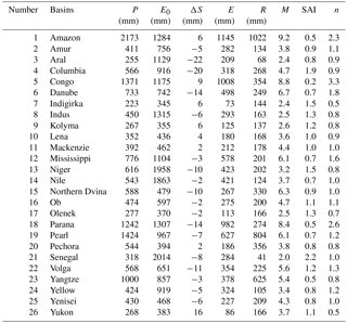
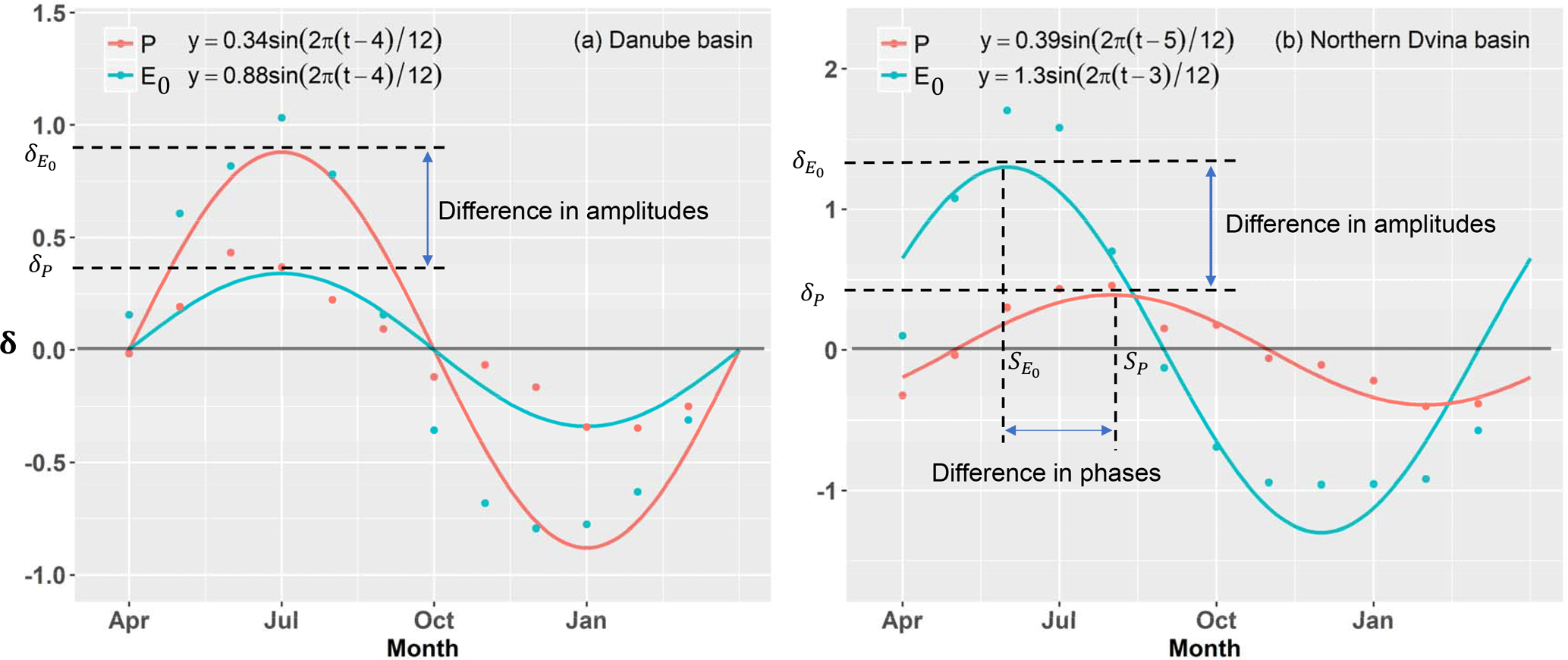
Figure 1 Two examples showing the mismatch between long-term monthly precipitation (P) and potential evapotranspiration (E₀), in terms of (a) seasonal amplitudes (δ_P, ${\mathit{\delta }}_{E_{\mathrm{0}}}$) and (b) phase shift (S_P, $S_{E_{\mathrm{0}}}$).

3 Methods

3.1 The Budyko framework at annual scale

The Budyko framework has been widely used in the assessment of impacts of climate and vegetation variations on the hydrological cycle. There are several analytical equations proposed under the Budyko framework, among which the function deduced by Choudhury (1999) and Yang et al. (2008) has been identified to perform better than other equations (Zhou et al., 2015). The function can be expressed as follows:

$$\begin{array}{}\text{(1)}& E={\displaystyle \frac{P{E}_{\mathrm{0}}}{{\left(P^n+E_{\mathrm{0}}^n\right)}^{\mathrm{1}/n}}},\end{array}$$

where n is the controlling parameter of the Choudhury–Yang equation.

The basin stores precipitation first and then releases it as runoff and evapotranspiration (Biswal, 2016). Affected by water storage changes, E is never equal to the difference between P and R for a short time interval. Previous studies have found that storage changes have impacts on water balance at the annual scale (Donohue et al., 2012). To consider the influence of variation in water storage, Wang (2012) suggested to use effective precipitation (P_e), i.e., $P_{\mathrm{e}}=P-\mathrm{\Delta }S$, to replace precipitation in the water–energy balance. As a result, using the P_e, the Choudhury and Yang equation can be extended in a short timescale:

$$\begin{array}{}\text{(2a)}& {\displaystyle }& {\displaystyle }R=P_{\mathrm{e}}-{\displaystyle \frac{P_{\mathrm{e}}{E}_{\mathrm{0}}}{{\left(P_{\mathrm{e}}^n+E_{\mathrm{0}}^n\right)}^{\mathrm{1}/n}}},\text{(2b)}& {\displaystyle }& {\displaystyle }E={\displaystyle \frac{P_{\mathrm{e}}{E}_{\mathrm{0}}}{{\left(P_{\mathrm{e}}^n+E_{\mathrm{0}}^n\right)}^{\mathrm{1}/n}}}.\end{array}$$

Parameter n controls the shape of the Budyko curve and can be calibrated by minimizing the mean absolute error (MAE) of runoff (Legates and McCabe, 1999; Yang et al., 2007). Parameter n is a catchment characteristic parameter which is mainly related to the underlying conditions (i.e., topography and soil), climate conditions and vegetation cover (Liu et al., 2017a; Yang et al., 2009; Zhang et al., 2016c). The underlying characteristics are relatively stable during a short time interval, while climate and vegetation might undergo considerable variations, which can lead to the change in parameter n. As a result, vegetation dynamics and climate variability were applied to simulate n and assess their impact on runoff and evapotranspiration.

The vegetation coverage (M), which is the fraction of land surface covered with green vegetation in the region, can be calculated as follows (Gutman and Ignatov, 1998):

$$\begin{array}{}\text{(3)}& M=(\mathrm{NDVI}-{\mathrm{NDVI}}_{\min })/({\mathrm{NDVI}}_{\max }-{\mathrm{NDVI}}_{\min }),\end{array}$$

where NDVI_max and NDVI_min represent the dense green vegetation and bare soil with NDVI_max=0.80 and NDVI_min=0.05, respectively (Li et al., 2013; Ning et al., 2017; Yang et al., 2009).

3.2 Seasonality and asynchrony of water and energy

The seasonality of P and E₀, which are mainly controlled by solar radiation, follows a sine distribution (Milly, 1994; Woods, 2003; Berghuijs and Woods, 2016):

$$\begin{array}{}\text{(4a)}& {\displaystyle }& {\displaystyle }P\left(t\right)=\stackrel{\mathrm{‾}}{P}\left(\mathrm{1}+{\mathit{\delta }}_P\sin \left({\displaystyle \frac{\mathrm{2}\mathit{\pi }}{\mathit{\tau }}}{\displaystyle \frac{t}{\mathrm{12}}}\right)\right),\text{(4b)}& {\displaystyle }& {\displaystyle }{E}_{\mathrm{0}}\left(t\right)=\stackrel{\mathrm{‾}}{E_{\mathrm{0}}}\left(\mathrm{1}+{\mathit{\delta }}_{E_{\mathrm{0}}}\sin \left({\displaystyle \frac{\mathrm{2}\mathit{\pi }}{\mathit{\tau }}}{\displaystyle \frac{t}{\mathrm{12}}}\right)\right),\end{array}$$

where t is the time (months), and P(t) and E₀ (t) are the monthly P and E₀ with the annual mean value of $\stackrel{\mathrm{‾}}{P}$ and of $\stackrel{\mathrm{‾}}{E_{\mathrm{0}}}$, respectively. The quantities δ_P and ${\mathit{\delta }}_{E_{\mathrm{0}}}$ are dimensionless seasonal amplitudes, which can be calibrated by minimizing MAE. The quantity τ is the cycle of seasonality, with 6 months in the tropics and 1 year outside the tropics. The origin of time (t=0) was fixed in April in the previous studies (Milly, 1994; Woods, 2003; Ning et al., 2017). As a result, if the δ_P (${\mathit{\delta }}_{E_{\mathrm{0}}})$ was positive, the month with maximum monthly P (E₀) would appear in July, which corresponds to Northern Hemisphere (e.g., Fig. 1a); while the Southern Hemisphere would show a January maximum with negative ${\mathit{\delta }}_P({\mathit{\delta }}_{E_{\mathrm{0}}}$). Considering the difference between seasonal P and E₀, Wood et al. (2003) defined a climate seasonality index by combining Eq. (4):

$$\begin{array}{}\text{(5)}& \mathrm{SI}=\mathrm{|}{\mathit{\delta }}_P-{\mathit{\delta }}_{E_{\mathrm{0}}}\mathrm{DI}\mathrm{|},\end{array}$$

where DI is the dryness index $\left(\frac{\stackrel{\mathrm{‾}}{E_{\mathrm{0}}}}{\stackrel{\mathrm{‾}}{P}}\right)$.

Equations (4)–(5) were applied to represent the mismatch between water and energy (e.g., Ning et al., 2017). However, the following two issues still need to be considered: (1) the effect of local climate and catchment characteristics – the phase of seasonal P and E₀ may be not entirely consistent with that of solar radiation – and (2) the phases between seasonal P and E₀ cannot always be consistent in a specific basin, such as the Northern Dvina basin (Fig. 1b). The values of E for two basins with the same annual mean P, E₀, δ_P and ${\mathit{\delta }}_{E_{\mathrm{0}}}$ can be different if the phases of seasonal P and E₀ are in mismatch. As a result, the phase shifts of P (S_P) and $E_{\mathrm{0}}(S_{E_{\mathrm{0}}}$) should be considered in the sine function (Berghuijs and Woods, 2016):

$$\begin{array}{}\text{(6a)}& {\displaystyle }& {\displaystyle }P\left(t\right)=\stackrel{\mathrm{‾}}{P}\left(\mathrm{1}+{\mathit{\delta }}_P\sin \left({\displaystyle \frac{\mathrm{2}\mathit{\pi }}{\mathit{\tau }}}{\displaystyle \frac{t-S_P}{\mathrm{12}}}\right)\right),\text{(6b)}& {\displaystyle }& {\displaystyle }{E}_{\mathrm{0}}\left(t\right)=\stackrel{\mathrm{‾}}{E_{\mathrm{0}}}\left(\mathrm{1}+{\mathit{\delta }}_{E_{\mathrm{0}}}\sin \left({\displaystyle \frac{\mathrm{2}\mathit{\pi }}{\mathit{\tau }}}{\displaystyle \frac{t-S_{E_{\mathrm{0}}}}{\mathrm{12}}}\right)\right).\end{array}$$

As shown in Fig. 2, Eq. (6) with a fitted phase performed much better in simulating monthly P and E₀ than Eq. (4) with a fixed phase, with R² larger than 0.89 for the former but smaller than 0.64 for the latter.

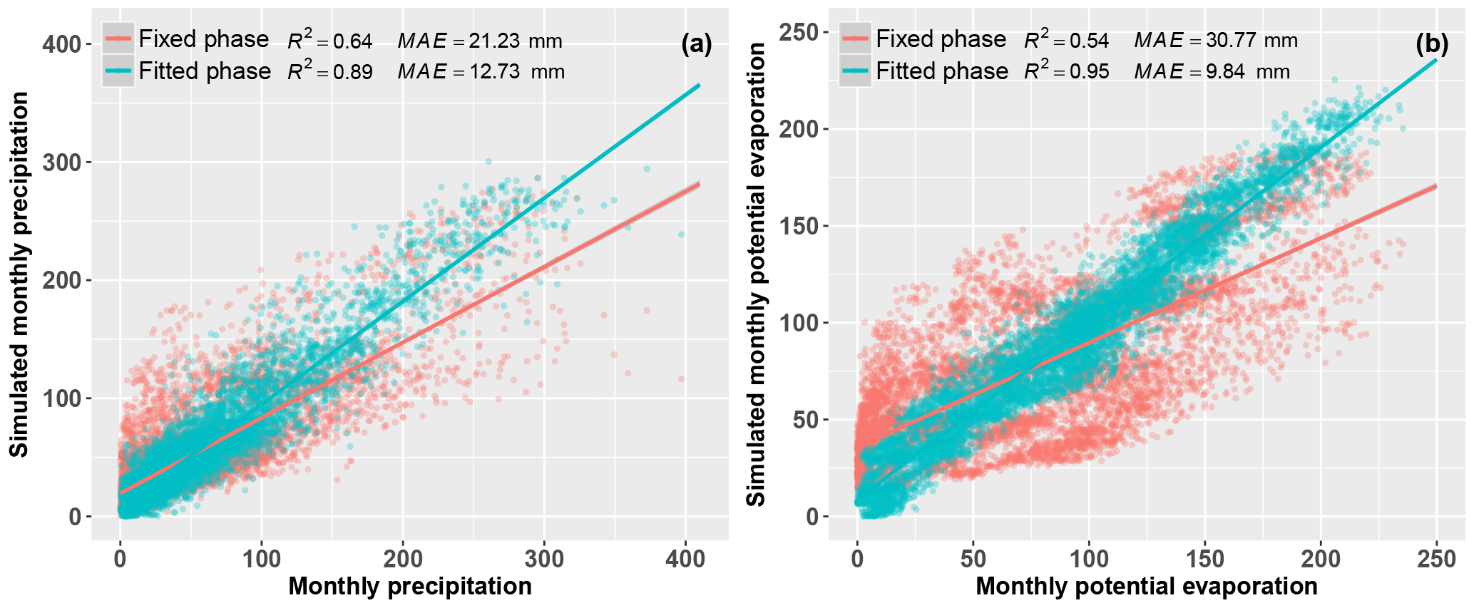
Figure 2 Comparing the observed and simulated monthly precipitation and potential evapotranspiration, using the sine function with a fixed phase (i.e., Eq. 4) and fitted phase (i.e., Eq. 6). Note that each point represents 1-month data based on the combined dataset from 26 global large basins.

To fully reflect the difference between water and energy, it is necessary to consider not only the seasonal amplitude difference between P and E₀, but also the phase difference (i.e., asynchrony) between them (Fig. 1b). Therefore, an improved climate index describing the difference between water and energy needs to be developed with the consideration of seasonality and asynchrony of P and E₀. Based on Eq. (6), we further deduced the following equations to express the difference between P and E₀:

$$\begin{array}{ll}{\displaystyle \frac{P\left(t\right)-E_{\mathrm{0}}\left(t\right)}{\stackrel{\mathrm{‾}}{P}}}& {\displaystyle }=\left(\mathrm{1}-\mathrm{DI}\right)+\left({\mathit{\delta }}_P\sin \left({\displaystyle \frac{\mathrm{2}\mathit{\pi }}{\mathit{\tau }}}{\displaystyle \frac{t-S_P}{\mathrm{12}}}\right)\right.\\ {\displaystyle }& {\displaystyle }\left.-\mathrm{DI}{\mathit{\delta }}_{E_{\mathrm{0}}}sin\left({\displaystyle \frac{\mathrm{2}\mathit{\pi }}{\mathit{\tau }}}{\displaystyle \frac{t-S_{E_{\mathrm{0}}}}{\mathrm{12}}}\right)\right)\\ \text{(7)}& {\displaystyle }& {\displaystyle }=\left(\mathrm{1}-\mathrm{DI}\right)+{\left(a^{\mathrm{2}}+b^{\mathrm{2}}\right)}^{\mathrm{1}/\mathrm{2}}\sin \left({\displaystyle \frac{\mathrm{2}\mathit{\pi }}{\mathit{\tau }}}{\displaystyle \frac{t}{\mathrm{12}}}+\mathit{\phi }\right)\end{array}$$

where $a={\mathit{\delta }}_P\cos \frac{\mathrm{2}\mathit{\pi }}{\mathit{\tau }}\frac{S_P}{\mathrm{12}}-\mathrm{DI}{\mathit{\delta }}_{E_{\mathrm{0}}}\cos \frac{\mathrm{2}\mathit{\pi }}{\mathit{\tau }}\frac{S_{E_{\mathrm{0}}}}{\mathrm{12}}$, $b=-{\mathit{\delta }}_P\sin \frac{\mathrm{2}\mathit{\pi }}{\mathit{\tau }}\frac{S_P}{\mathrm{12}}+\mathrm{DI}{\mathit{\delta }}_{E_{\mathrm{0}}}\sin \frac{\mathrm{2}\mathit{\pi }}{\mathit{\tau }}\frac{S_{E_{\mathrm{0}}}}{\mathrm{12}}$, $\mathit{\phi }=\arctan (b/a)$. Similar to Milly (1994), we defined a SAI to reflect the mismatch between water and energy in terms of the magnitude and phase difference between P and E₀:

$$\begin{array}{ll}{\displaystyle }\mathrm{SAI}& {\displaystyle }={\left(a^{\mathrm{2}}+b^{\mathrm{2}}\right)}^{\mathrm{1}/\mathrm{2}}\\ {\displaystyle }& {\displaystyle }=\left({\mathit{\delta }}_P^{\mathrm{2}}-\mathrm{2}{\mathit{\delta }}_P{\mathit{\delta }}_{E_{\mathrm{0}}}\mathrm{DI}\cos \left({\displaystyle \frac{\mathrm{2}\mathit{\pi }}{\mathit{\tau }}}{\displaystyle \frac{S_P-S_{E_{\mathrm{0}}}}{\mathrm{12}}}\right)\right.\\ \text{(8)}& {\displaystyle }& {\displaystyle }+{\left.({\mathit{\delta }}_{E_{\mathrm{0}}}\mathrm{DI}{)}^{\mathrm{2}}\right)}^{\mathrm{1}/\mathrm{2}}.\end{array}$$

The SI value calculated by Eq. (5) was an exceptional case for P and E₀ in the same phase shifts. A larger SAI implies a greater difference between P and E₀ in the year. Besides, SAI followed the following three scenarios: (1) SAI<1−DI, given a wet climate with P(t) > E₀ (t) across the whole seasonal cycle (Fig. 3a); (2) SAI<DI−1, given a dry climate with P(t) < E₀ (t) across the whole seasonal cycle (Fig. 3b); (3) $\mathrm{SAI}\ge \mathrm{|}\mathrm{DI}-\mathrm{1}\mathrm{|}$, given that a larger SAI implies more surplus of P for the wet season with P(t) > E₀ (t) (Fig. 3c).

3.3 Contributions of SAI and other factors to R and E

From Eq. (2), using a total differential method, we can redefine the total differential of R and E for any timescale by introducing effective precipitation (P_e):

$$\begin{array}{}\text{(9a)}& {\displaystyle }& {\displaystyle }\mathrm{d}R\approx {\displaystyle \frac{\partial R}{\partial P_{\mathrm{e}}}}\mathrm{d}{P}_{\mathrm{e}}+{\displaystyle \frac{\partial R}{\partial E_{\mathrm{0}}}}\mathrm{d}{E}_{\mathrm{0}}+{\displaystyle \frac{\partial R}{\partial n}}\mathrm{d}n,\text{(9b)}& {\displaystyle }& {\displaystyle }\mathrm{d}E\approx {\displaystyle \frac{\partial E}{\partial P_{\mathrm{e}}}}\mathrm{d}{P}_{\mathrm{e}}+{\displaystyle \frac{\partial E}{\partial E_{\mathrm{0}}}}\mathrm{d}{E}_{\mathrm{0}}+{\displaystyle \frac{\partial E}{\partial n}}\mathrm{d}n.\end{array}$$

The climatic elasticity of evapotranspiration changes to the changes in precipitation, potential evapotranspiration and n can be separately be expressed as ${\mathit{\epsilon }}_{P_{\mathrm{e}}}=\frac{P_{\mathrm{e}}}{E}\frac{\partial f}{\partial P_{\mathrm{e}}}$, ${\mathit{\epsilon }}_{E_{\mathrm{0}}}=\frac{E_{\mathrm{0}}}{E}\frac{\partial f}{\partial E_{\mathrm{0}}}$, ${\mathit{\epsilon }}_n=\frac{n}{E}\frac{\partial f}{\partial n}$. The climatic elasticity of runoff changes is similar to the climatic elasticity evapotranspiration changes. The difference operator (d) in Eqs. (9a) and (9b) refers to the difference of a variable before and after change points of R and E, respectively. It is worth noting that Eq. (9) is derived by the first-order approximation of Taylor expansion. When the changes in dP_e, dE₀ and dn are small, the error from approximation can be ignored. However, due to ignoring the higher orders of the Taylor expansion, the error will increase as the changes increase (Yang et al., 2014a, b; Zhou et al., 2016).

The relative contribution (C) of P_e, E₀ and n to the R and E changes can be obtained as follows:

$$\begin{array}{ll}{\displaystyle }& {\displaystyle }{C}_{P_{\mathrm{e}}}={\displaystyle \frac{I_{p_{\mathrm{e}}}}{\mathrm{|}{I}_P\mathrm{|}+\mathrm{|}{I}_{E_{\mathrm{0}}}\mathrm{|}+\mathrm{|}{I}_n\mathrm{|}}},C_{E_{\mathrm{0}}}={\displaystyle \frac{I_{E_{\mathrm{0}}}}{\mathrm{|}{I}_P\mathrm{|}+\mathrm{|}{I}_{E_{\mathrm{0}}}\mathrm{|}+\mathrm{|}{I}_n\mathrm{|}}},\\ \text{(10)}& {\displaystyle }& {\displaystyle }{C}_n={\displaystyle \frac{I_n}{\mathrm{|}{I}_P\mathrm{|}+\mathrm{|}{I}_{E_{\mathrm{0}}}\mathrm{|}+\mathrm{|}{I}_n\mathrm{|}}}\end{array}$$

$I_{p_{\mathrm{e}}},I_{E_{\mathrm{0}}}$ and I_n denote, respectively, the impacts of P_e, E₀ and n on R or E, which can be expressed by $\frac{\partial E}{\partial P_{\mathrm{e}}}\mathrm{d}{P}_{\mathrm{e}}$, $\frac{\partial E}{\partial E_{\mathrm{0}}}\mathrm{d}{E}_{\mathrm{0}}$ and $\frac{\partial E}{\partial n}\mathrm{d}n$. After getting the contribution of n to the R and E variations, we can further assess the impacts of M and SAI on the variation in R and E, based on the semi-empirical model of n in terms of M and SAI. Following Ning et al. (2017), using the total differential method, the changes in parameter n can be expressed as follows:

$$\begin{array}{}\text{(11)}& \mathrm{d}n\approx {\displaystyle \frac{\partial n}{\partial \mathrm{SAI}}}\mathrm{dSAI}+{\displaystyle \frac{\partial n}{\partial M}}\mathrm{d}M.\end{array}$$

Then, the relative contributions of SAI (C_SAI) and M (C_M) to the changes in parameter n can be obtained. Combining with the contribution of n to the R and E changes, the relative contributions of SAI and M to the variations in R and E can be obtained:

$$\begin{array}{}\text{(12)}& C_{\mathrm{SAI}}=C_n\times C\mathit{\_}\mathrm{SAI},C_M=C_n\times C\mathit{\_}M.\end{array}$$

4 Results

4.1 Performance of the proposed SAI in the Budyko framework

Figure 2 shows that Eq. (6) with SAI has a better performance in simulating P and E₀ than Eq. (4) with SI. Here we further assessed the performance of these two indices, by comparing with the controlling parameter n in the Budyko framework. Parameter n for each year was first calibrated by Eq. (2). The calibrated parameter n was called optimized n. For the representativeness of the relation between n and other factors, analysis was done at a larger spatial scale with different climate conditions by combining data from 26 global large basins (Fig. 4).

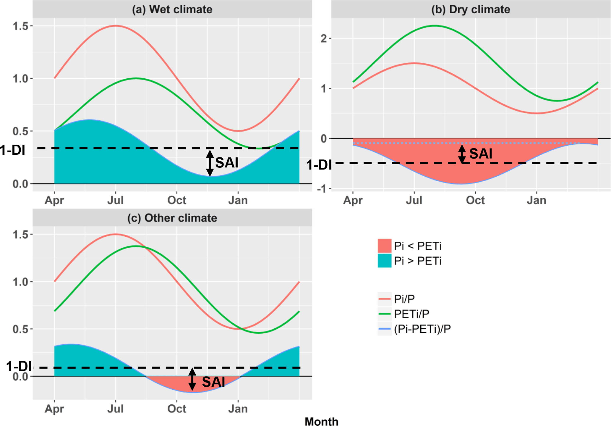
Figure 3 Examples of three scenarios for the mismatch between water and energy in terms of the relationship of SAI to 1-DI. (a) SAI smaller than 1-DI, implying P larger than PET for the whole year. (b) SAI smaller than DI-1, implying P smaller than PET for the whole year. (c) SAI smaller than 1-DI, implying a larger SAI means more surplus of P. The shaded areas represent the difference between precipitation and potential evapotranspiration, which is equal to $\left(\mathrm{1}-\mathrm{DI}\right)+\mathrm{SAI}\sin \left(\frac{\mathrm{2}\mathit{\pi }}{\mathit{\tau }}\frac{t}{\mathrm{12}}+\mathit{\phi }\right)$.

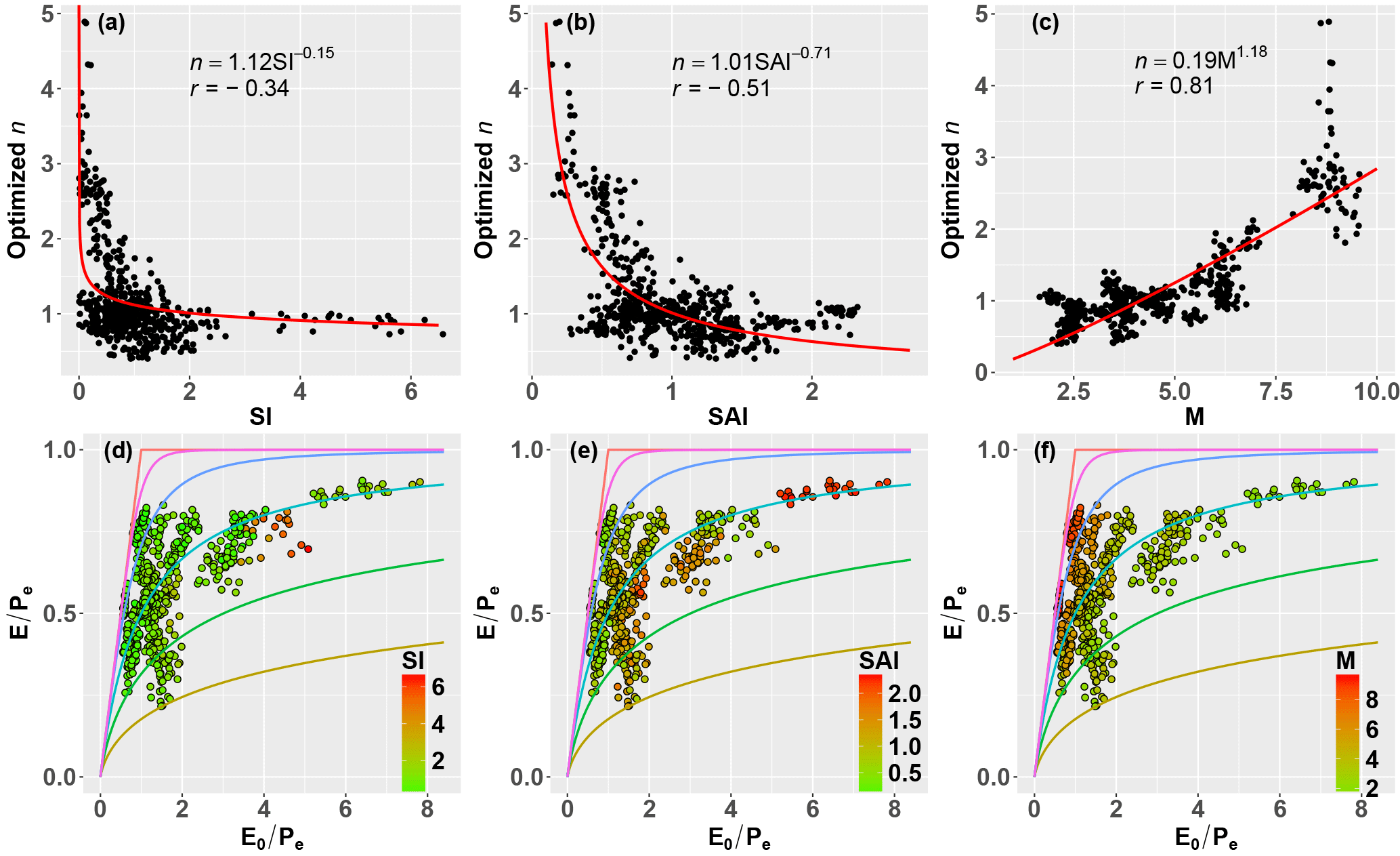
Figure 4 Relationship between optimized n and (a) SI, (b) SAI and (c) M. (d–f) Distribution of evapotranspiration ratio (E ∕ P_e) as a function of the aridity index (E₀ ∕ P_e), classified by 26 global large river basins at annual scale. The Budyko curves from the top down are derived from Eq. (2b) with n=∞, n=5, n=2, n=1, n=0.6 and n=0.4, respectively. Note that each point represents 1 year based on the combined dataset from 26 global large basins.

The correlation coefficient (r) between SI and optimized n was −0.34 (Fig. 4a). If the asynchrony of seasonal P and E₀ was considered in SI, i.e., SAI, the correlation coefficient increased noticeably with r of −0.51 (Fig. 4b). To further assess the impact of SAI on the fluvial water balance, we also analyzed the roles of SAI in the Budyko framework. As shown in Fig. 4e, a larger n value was related to a higher evapotranspiration ratio for a given aridity index, and as SAI increased, the value of controlling parameter n tended to decrease. In other words, catchments with a larger SAI had a lower evapotranspiration ratio given the same aridity index. This result is similar to the finding by Zhang et al. (2015), who found that a larger snow ratio caused a higher runoff index given the same dryness index. In contrast, this relationship is not distinct for SI (Fig. 4d). In addition, the SAI can explain 51 % of the annual variance of parameter n, while the SI just explains 22 % (Fig. 4a and b). In short, although SI showed a significant relationship with n, SAI considering both seasonality and asynchrony of P and E₀ was more applicable to represent the difference between water and energy and performed better in the simulation of n in the Budyko model.

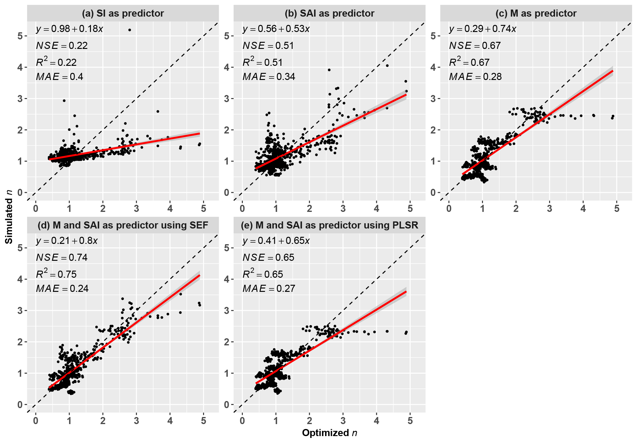
Figure 5 Optimized (calibrated) n versus simulated n modeled by (a) SI, (b) SAI, (c) M, (d) M and SAI using the semi-empirical formula (SEF, Eq. 14), and (e) M and SAI using the partial least square regression (PLSR). Note that each point represents one year based on the combined dataset from 26 global large basins.

The variation in SAI is also sensitive to climate variability. As shown in Fig. 6, the climate elasticities of evapotranspiration to precipitation and parameter n increased with SAI, whereas the elasticity of evapotranspiration to potential evapotranspiration decreased with SAI, which implies that the variation in evapotranspiration in the catchments with a higher SAI were more sensitive to the changes in precipitation and parameter n, but less sensitive to the changes in potential evapotranspiration.

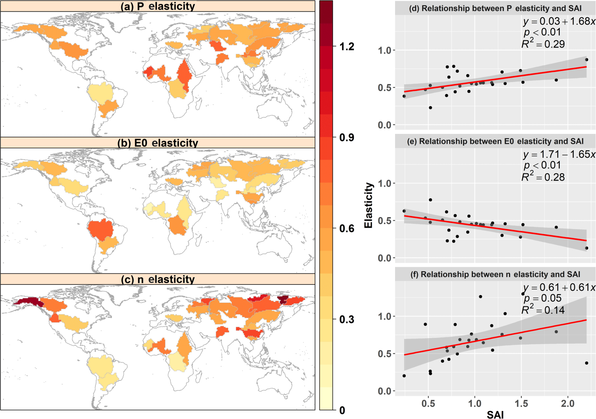
Figure 6 The climatic elasticity of evapotranspiration to the changing precipitation, potential evaporation and other factors represented by controlling parameter n in the 26 global large river basins, and its relations with the climate seasonality and asynchrony index (SAI). Note that each point represents one of the 26 global large basins.

4.2 A semi-empirical formula for parameter n

Previous studies have found that vegetation cover is closely related to the spatial variation in n in different regions (e.g., Li et al., 2013). However, the new finding in this study is that vegetation dynamics (M) also have a significant impact on the temporal variation in annual values of the parameter n (Figs. 4c and 5c) and evapotranspiration ratio (Fig. 4f). Nevertheless, the simulation accuracy of n can be further improved, particularly at the high end. As mentioned above, SAI has a significant impact on the variation in n. Therefore, based on the results obtained by Li et al. (2013), it is possible to develop a more dynamic model to capture the spatiotemporal variation in parameter n and improve the simulation of n by incorporating SAI into the empirical model.

Following the phenomenological considerations and the relationships demonstrated in Fig. 4b and c, the limiting conditions of SAI and M were achieved: (1) if $\mathrm{SAI}\to +\mathrm{\infty }$, which indicates that the match of P and E₀ tends to be the worst, and thus R→P and E→0, i.e., n→0; (2) when M↑, then E↑, which has been demonstrated by previous studies (i.e., Yang et al., 2009; Li et al., 2013), and thus n↑, which can also be found in Fig. 4c and f. Based on these limiting conditions, a semi-empirical formula (SEF) for parameter n was obtained as follows:

$$\begin{array}{}\text{(13)}& n=a{\mathrm{SAI}}^b{M}^c,\end{array}$$

where a and c are positive regression coefficients and b is negative. Nonlinear least squares can be used to estimate the values of a, b and c, based on n calibrated from measured data. Then, the final equation was as follows:

$$\begin{array}{}\text{(14)}& n=\mathrm{0.27}{\mathrm{SAI}}^{-\mathrm{0.30}}{M}^{\mathrm{0.90}}.\end{array}$$

As shown in Fig. 5d, the simulated n calculated by SEF match well with the optimized n with R² of 0.75 and MAE of 0.24. In addition, the Eq. (13) has also been verified in each catchment among the 26 basins (Table S1 in the Supplement). The RMSE and MAE for each catchment is relatively small, with mean values of 12.0 and 14.8 mm, respectively. Except for basins 3, 5 and 26, the R² values for simulation of R in each catchment are larger than 0.5. These results indicated that the M and SAI as well as the semi-empirical formula can explain well the variability of the controlling parameter n.

In addition to the SEF, linear regression is often applied to simulate n. For example, taking NDVI, latitude and topographic index as explanatory variables, Xu et al. (2013) applied multiple linear regression to estimate the spatial variation in n for the global large river basins. Considering the multicollinearity issue, the partial least square regression (PLSR) was used in this study. As shown in Fig. 5e, the values of Nash–Sutcliffe efficiency (NSE) and mean absolute error (MAE) of the simulated n by using PLSR were 0. 65 and 0.27 respectively, which was not as good as the performance of the semi-empirical formula. Therefore, the SEF was a better choice not only for simulation but also for explaining the physical meaning.

Cross-validation was used to validate the semi-empirical equation. The dataset for one basin was used for validation, and the datasets for the remaining 25 basins were used for calibration. Then the cross-validation process is repeated 26 times, with each of the 26 basins used once as validation. Parameter n for the validation basin was simulated by the semi-empirical formula obtained from the other 25 basins. The calibrated parameters for each basin can be found in Table S2. Subsequently, based on annual P_e, E₀ and simulated annual parameter n, simulated annual R and E were calculated using Eq. (2). The simulated annual R and E for each validated basin were combined to compare with the observed R and E, respectively (Fig. 7). As shown in Fig. 7a and b, the simulated annual R and E that estimated by Budyko model with cross-validation parameter n showed a remarkable agreement with the observed ones, with NSE larger than 0.89 and MAE smaller than 50.52 mm, which is close to the simulation accuracy of these estimated by Budyko model with simulated parameter n by using the semi-empirical formula (i.e., Eq. 14, Fig. 7c and d). These results indicated that the semi-empirical formula expressed the spatiotemporal variation in parameter n, and the proposed Eq. (2) with simulated parameter n was reliable for the simulation of annual R and E.

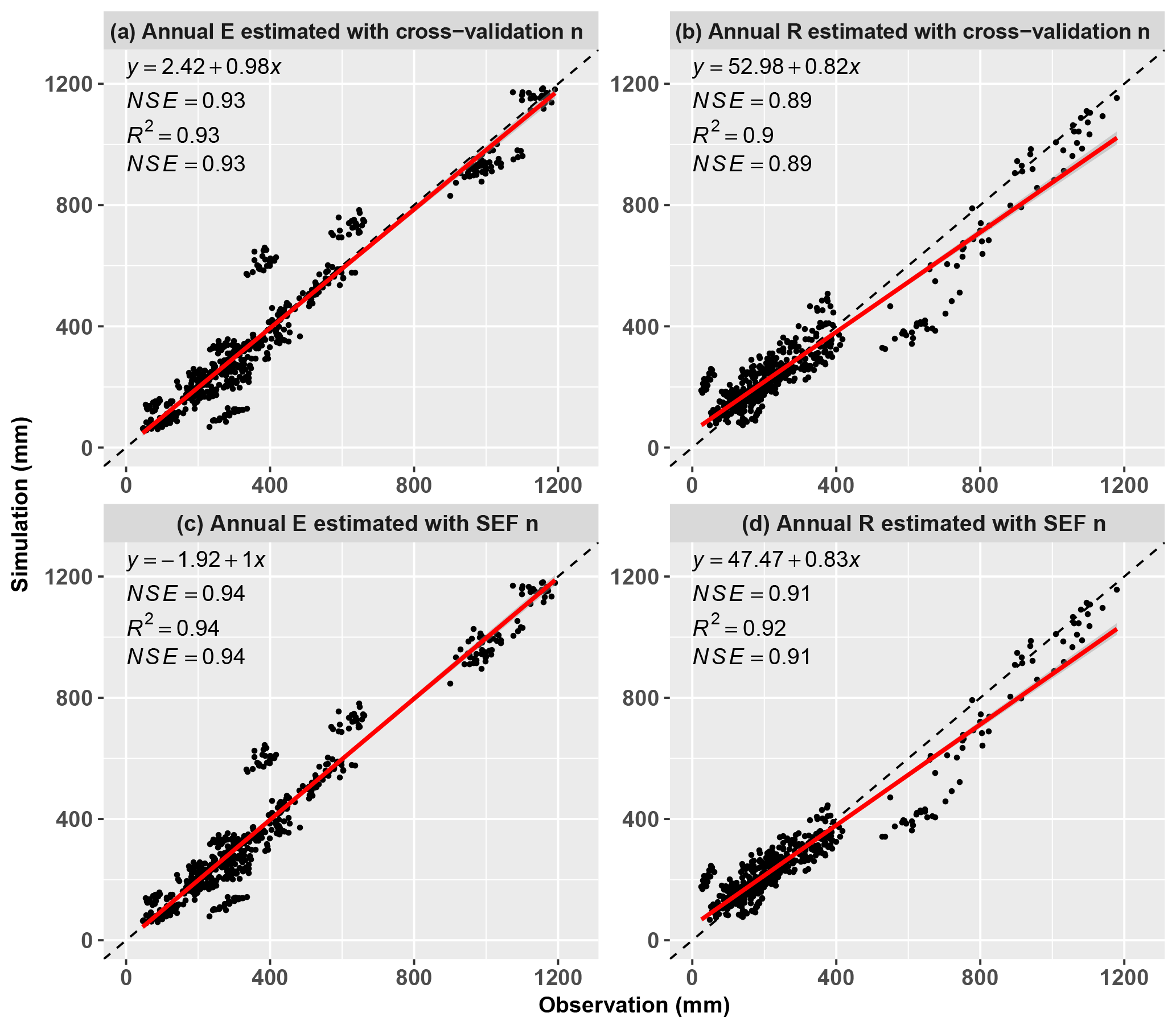
Figure 7 The observed E and R vs. the simulated E and R estimated by Budyko model with simulated parameter n by (a–b) Eq. (13) with cross-validation method and (c–d) semi-empirical formula (SEF, Eq. 14).

4.3 Contributions of SAI and other factors to R and E changes

To further assess the impact of SAI on the water balance, here we quantified the contributions of SAI and other factors, i.e., P_e, E₀ and M, on the changes in R and E before and after change point. We used an ordered clustering test, a Pettitt test method and a change point analysis method for the “at most one change” (AMOC) method to detect the change points of R. To avoid possible uncertainty within results based on the individual method, the assembled change points were confirmed with more than one method. If the results for all the three methods are different, the median change point would be selected (Liu et al., 2017a). Based on the change points of R and the changes rates of P_e, E₀, M and SAI before and after change points (Table S3), the contributions of these four factors to R and E were assessed (Figs. 8 and 9; Table S3).

As can be seen from Fig. 8a and c, the P_e changes controlled the variation in R in most basins, with 18 of the 26 selected basins. The absolute value of contributions of P_e changes to R changes ranged from 11 % to 96 %, with the median value at 61 % for the 26 basins (Fig. 8b). In addition to the P_e changes, the SAI change was also an important factor for the R change with the median absolute contribution at 16 %. SAI was the dominant factor with the maximum contribution to R changes in six rivers, such as Yangtze, Yellow, Aral, Northern Dvina, Congo and Mississippi basins. The E₀ changes reduce the R in 24 of the 26 basins (Table S4). The E₀ changes had a limited impact on the R changes with the median absolute contribution of 8 %. However, it is the dominant factor for R changes in Parana River basins.

Figure 8 Absolute value of contributions to the long-term mean changes in runoff (before and after change point of R) from P_e, SAI, M and E₀ changes. The distribution ranges of absolute values of contribution for each factor are shown in (b) and the number of basins dominated by each factor with the largest relative contribution is summarized in (c).

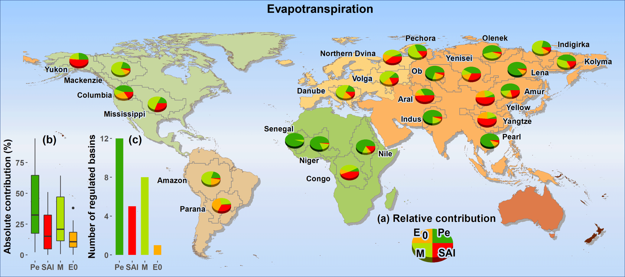
Figure 9 The same as Fig. 8 but for relative contribution to the changes in evapotranspiration.

The dominant factors of E changes were different from those of R changes (Fig. 9). Both the SAI and M changes had remarkable impacts on the E changes, which were the dominant factors for the E changes within eight and five basins, respectively. Also, the contributions of SAI and M changes to E changes were larger than those to R changes with the median absolute contributions of 21 % and 28 %, respectively. Accordingly, the contribution of P_e to E changes was weaker than that to R changes, the median of which dropped from 61 % to 32 %.

In summary, P_e was the key controlling factor for R and E in most river basins. SAI was the dominant factor for both R and E mainly in East Asian subtropical monsoon zones because of the monsoon variability (Cook et al., 2010), such as Yangtze and Yellow River basins. SAI, M and E₀ have larger impacts on the E changes than R changes do, while P has stronger impacts on R changes than E changes do.

5 Discussion

It has been found that both vegetation coverage and climate seasonality have impacts on water balance (Chen et al., 2013; Li et al., 2013; Zeng and Cai, 2016; Abatzoglou and Ficklin, 2017; Ning et al., 2017; Zhang et al., 2016a). Li et al. (2013) found that long-term vegetation coverage was closely related to the spatial variation in the calibrated parameter of the Budyko model in global river basins. However, vegetation dynamics also influenced the temporal variation in parameter n, but the relationship is yet to be verified over a larger spatial range (Zhang et al., 2016c; Ning et al., 2017). Results of this study confirmed that the vegetation dynamics had a significant impact on both spatial and temporal variations in the controlling parameter n at the global scale.

The seasonality index represents the amplitude difference of seasonal P and E₀, but does not include the phase difference of seasonal P and E₀. Investigating the water balance across the Loess Plateau in China, Ning et al. (2017) found that the seasonal index was closely related to the controlling parameter. In this study, however, SI showed a worse correlation with the variation in n in the 26 large global river basins than those in Loess Plateau. All catchments selected by Ning et al. (2017) were in the monsoon climate zone, where water and energy are strongly coupled, so the seasonality of P and E₀ in most catchments was in the same phase. Hence, the asynchrony of water and energy was nonexistent and had a limited impact on the variation in n. In contrast, the basins selected in this study covered a large spatial scale with a wide range of climate types. Most basins had different phases between seasonal P and E₀, such as the Northern Dvina, with the phase differences larger than 2 months. The amplitude difference between seasonal P and E₀ cannot adequately represent the difference between water and energy in the basins with out-of-phase P and E₀ (Hickel and Zhang, 2006). In this case, SAI, considering both amplitude and phase differences between seasonal of P and E₀, was proposed to reflect the difference between water and energy. Results showed that the proposed SAI had a significant impact on n and evapotranspiration radio, as well as the sensitively of evapotranspiration to the variation in precipitation, potential evapotranspiration and catchment characteristics. SAI can also be applied to other studies on water–energy balance.

In small-size catchments, interactions amongst climate variability, vegetation dynamics and water balance are more complex (Li et al., 2013). Many other factors, such as basins area, latitude, slope gradient, compound topographic index, and so on (Abatzoglou and Ficklin, 2017; Xu et al., 2013; Yang et al., 2009), have been identified as playing a role in the spatial distribution of n for small-size catchments. However, in this study, these factors had few changes at the annual timescale, so they were not considered in determining the annual variation in n. This study demonstrated that SAI and M play an important role in the spatiotemporal variation in n in large river basins, nevertheless, other factors should also be considered in the simulation of spatial variation in n for small-size catchments.

SAI was identified to have a great influence on the changes in R and E. In particular, the changes in both R and E for the two major rivers (i.e., Yangtze and Yellow River basins) in East Asian monsoon zones is mainly controlled by SAI. Hoyos and Webster (2007) found that the variation in monsoon systems has a remarkable effect on the climate seasonal pattern (Hoyos and Webster, 2007). Using the covariance of P and E₀ as an explanatory variable, Zeng and Cai (2016) indicated that the seasonality of P and E₀ had a significant impact on the E variation, such as in the Yangtze River basin. Their results are generally consistent with ours. To assess the impact of ecological restoration on runoff in the Loess Plateau of China, Liang et al. (2015) regarded the ecological restoration, i.e., vegetation dynamics, as the cause of changes in n. However, our results showed that SAI also played an important role in the changes in n, particularly for the East Asian subtropical monsoon zone.

Although SAI combined with M can capture the changes in n well (Fig. 5d), the impact of other factors represented by parameter n on the water balance not only includes SAI and M, but also the human influence, which has been verified by our previous study (Liu et al., 2017a). As a result, this may cause uncertainty in our findings. The human influences on R and E need to be further investigated.

6 Conclusions

In this study, a semi-empirical formula was developed to simulate the spatiotemporal variation in the controlling parameter n in the Budyko model. Influences of climate–vegetation factors on water balance were evaluated. The Choudhury–Yang equation modified by the effective precipitation is recommended to calibrate the controlling parameter n and to simulate evapotranspiration (E) and runoff (R), as well as their variation.

A climate seasonality and asynchrony index, i.e., SAI, is proposed to reflect the difference between water and energy. Results show that the optimized n has a much higher correlation with SAI than the existing SI, implying that the phase mismatch between seasonal water and energy should be considered in the impact assessment of water balance. In general, our results suggest that the catchments with a larger SAI usually have a larger evapotranspiration ratio given the same climatic and underlying condition, and the variation in evapotranspiration tends to be more sensitive to the changes in precipitation and landscape properties (parameter n), whereas it is less sensitive to the potential evapotranspiration in the catchments with larger SAI. Furthermore, this study confirms that vegetation dynamics (M) also play an important role in modifying the temporal variation in n at the annual scale. Based on SAI and M, a semi-empirical formula for the spatiotemporal variation in parameter n has been developed, and it performs well in the prediction of annual evapotranspiration and runoff.

Employing the developed semi-empirical formula, the contributions of SAI and M, as well as P_e and E₀, to the variation in E and R were assessed. Results show that precipitation is the first-order control on the R and E changes, and, secondly, SAI was found to control the changes in R and E in the subtropical monsoon regions of East Asia. SAI, M and E₀ have larger impacts on E than on R, whereas P_e has larger impacts on R.

The study assesses the influence of climate variability and vegetation dynamics on water balance, which highlights the role of climate seasonality and asynchrony as well as vegetation dynamics in the annual variation in n, and sheds new light on the difference in the contributions of climate–vegetation factors to the changes in R and E. This study can be useful for water–energy modeling, hydrological forecasting and water management.