the Creative Commons Attribution 4.0 License.
the Creative Commons Attribution 4.0 License.
 | 19 Jul 2018
Spatial patterns and characteristics of flood seasonality in Europe
Günter Blöschl
In Europe, floods are typically analysed within national boundaries and it is therefore not well understood how the characteristics of local floods fit into a continental perspective. To gain a better understanding at continental scale, this study analyses seasonal flood characteristics across Europe for the period 1960–2010.
From a European flood database, the timing within the year of annual maximum discharges or water levels of 4105 stations is analysed. A cluster analysis is performed to identify large-scale regions with distinct flood seasons based on the monthly relative frequencies of the annual maxima. The clusters are further analysed to determine the temporal flood characteristics within each region and the Europe-wide patterns of bimodal and unimodal flood seasonality distributions.
The mean annual timing of floods observed at individual stations across Europe is spatially well defined. Below 60∘ latitude, the mean timing transitions from winter floods in the west to spring floods in the east. Summer floods occurring in mountainous areas interrupt this west-to-east transition. Above 60∘ latitude, spring floods are dominant, except for coastal areas in which autumn and winter floods tend to occur. The temporal concentration of flood occurrences around the annual mean timing is highest in north-eastern Europe, with most of the floods being concentrated within 1–2 months.
The cluster analysis results in six spatially consistent regions with distinct flood seasonality characteristics. The regions with winter floods in western, central, and southern Europe are assigned to Cluster 1 (∼ 36 % of the stations) and Cluster 4 (∼ 10 %) with the mean flood timing within the cluster in late January and early December respectively. In eastern Europe (Cluster 3, ∼ 24 %), the cluster average flood occurs around the end of March. The mean flood timing in northern (Cluster 5, ∼ 8 %) and north-eastern Europe (Cluster 6, ∼ 5 %) is approximately in mid-May and mid-April respectively. About 15 % of the stations (Cluster 2) are located in mountainous areas, with a mean flood timing around the end of June. Most of the stations (∼ 73 %) with more than 30 years of data exhibit a unimodal flood seasonality distribution (one or more consecutive months with high flood occurrence). Only a few stations (∼ 3 %), mainly located on the foothills of mountainous areas, have a clear bimodal flood seasonality distribution.
This study suggests that, as a result of the consistent Europe-wide pattern of flood timing obtained, the geographical location of a station in Europe can give an indication of its seasonal flood characteristics and that geographical location seems to be more relevant than catchment area or catchment outlet elevation in shaping flood seasonality.
- Article
(19200 KB) - Full-text XML
-
Supplement
(73 KB) - BibTeX
- EndNote


Understanding the spatial and temporal characteristics of floods across Europe is important for improving our understanding of the flood generation mechanisms and hence for enabling better flood estimation and forecasts at European scale. River floods in Europe are caused by several processes. The most common naturally occurring river floods are driven by rainfall (including rain on snow) and snowmelt (sometimes combined with ice jams) and are modulated by soil moisture (e.g. Hall et al., 2014). Hence, depending on the time of the year (i.e. season) in which a flood peak occurs, one can infer the hydrological processes that are likely involved in the generation of the flood. For example, flood peaks occurring in late winter or early spring, together with rising air temperatures, can be inferred to be snowmelt-induced.
A better knowledge of the flood seasonality and hence the most probable flood generation processes can therefore assist in the identification of homogeneous regions with a dominant flood season, which is important for example for regional flood frequency analysis, the analysis of mixed flood frequency distributions, and in the identification and attribution observed changes in flood discharges. Additionally, such homogeneous regions can serve as a benchmark for the assessment of Europe-wide hydrological model output.
Previous research on flood seasonality in Europe has been limited by two main constraints. First, most scientific studies have focused on national scale or on smaller regions, which restricts the results to a relatively small and local set of flood-generating processes. For example, Beurton and Thieken (2009) determined three homogeneous flood regions in Germany when analysing the annual maximum floods (AMFs) of 481 gauging stations. Similarly, Cunderlik et al. (2004) found three main flood seasonality types in Great Britain by examining 268 sites. A few studies analysed flood seasonality at larger scales, for example Mediero et al. (2015) using 102 streamflow records within Europe, but with limited spatial coverage, and Blöschl et al. (2017) focusing on changes in flood seasonality. Second, most of the previous studies on flood seasonality focused on the mean date of the AMF occurrence and/or the temporal concentration of the floods around their mean date (e.g. Parajka et al., 2009 or Jeneiová et al., 2016 for both Austria and Slovakia), while the detailed characteristics of monthly flood seasonality distributions has rarely been studied in Europe. However, if unimodal, bimodal, or skewed seasonality distributions exist, the mean date of the AMFs can be misleading and can mask important insights into the flood-generating mechanisms (Ye et al., 2017). It is therefore important to report not only the mean date to characterise flood seasonality, but also to describe in detail the temporal flood seasonality characteristics.
To overcome the main research constraints, this paper examines the spatial and temporal patterns of flood seasonality at continental scale, using an extensive database that covers all climatic regions in Europe. The focus of this paper is on the identification of regions with similar seasonal flood characteristics and on the description of the full temporal distribution of the flood events within the year.
First, the study area and the European discharge dataset used in this study are presented, followed by the description of the analysis methods. In the results section, the spatial characteristics of the mean flood seasonality are presented together with an analysis of the seasonal flood characteristics across Europe. Spatial patterns and clusters are identified based on the monthly distribution of AMFs. The clusters are then examined in detail, focusing on their monthly flood seasonality characteristics and their spatial distribution. The paper concludes with a discussion of the results and the conclusion.
The hydrological data analysed here is based on the dataset presented by Hall et al. (2015) with subsequent updates. The initial database used in this study includes data from 5565 hydrometric stations from 38 data sources (see Supplement for details) located within 6.5∘ W–60∘ E and 29.25–69.25∘ N (Fig. 1).
Floods events are identified following the common definition as the highest (peak) event in a year (e.g. Garner et al., 2015; Hall et al., 2014). This does not necessary imply that the river overtops its banks and flows onto the floodplain during such a flood event. Following this definition, the dataset consists of the dates of annual maximum discharge or annual maximum water level (daily mean or instantaneous values). The maximum of each year is based on the calendar year (January to December) with a few exceptions, which are based on the respective countries' hydrological year (which can start in September, October, or November). Only the annual maxima are analysed here, as the long-term mean of the flood timing is more meaningful if a single flood peak per year is considered and, additionally, as in some areas and/or countries the restrictions in data access and licensing limits the availability of the data to the annual maxima only.
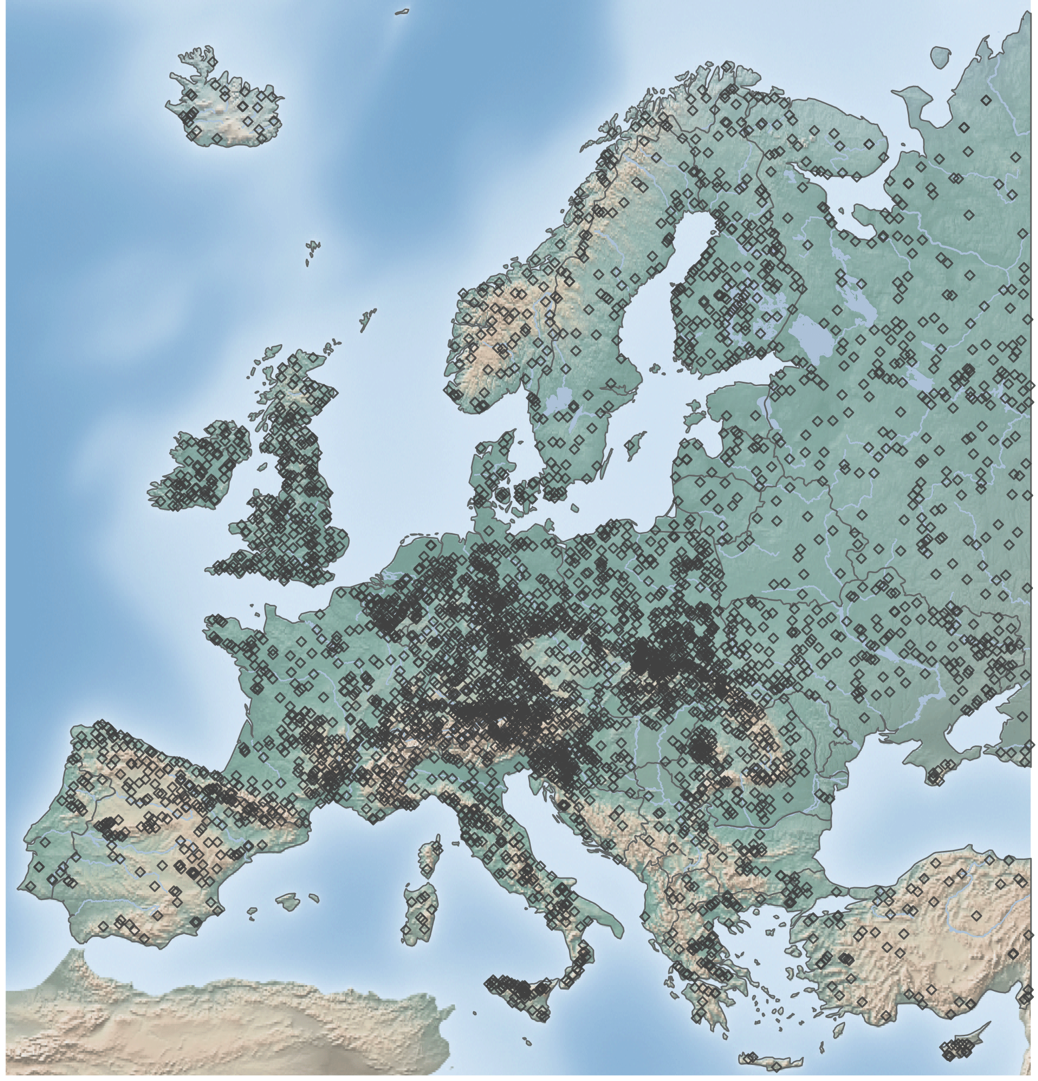
Figure 1Map of the study area, showing the topography and the location of the 4105 stations used in this study.
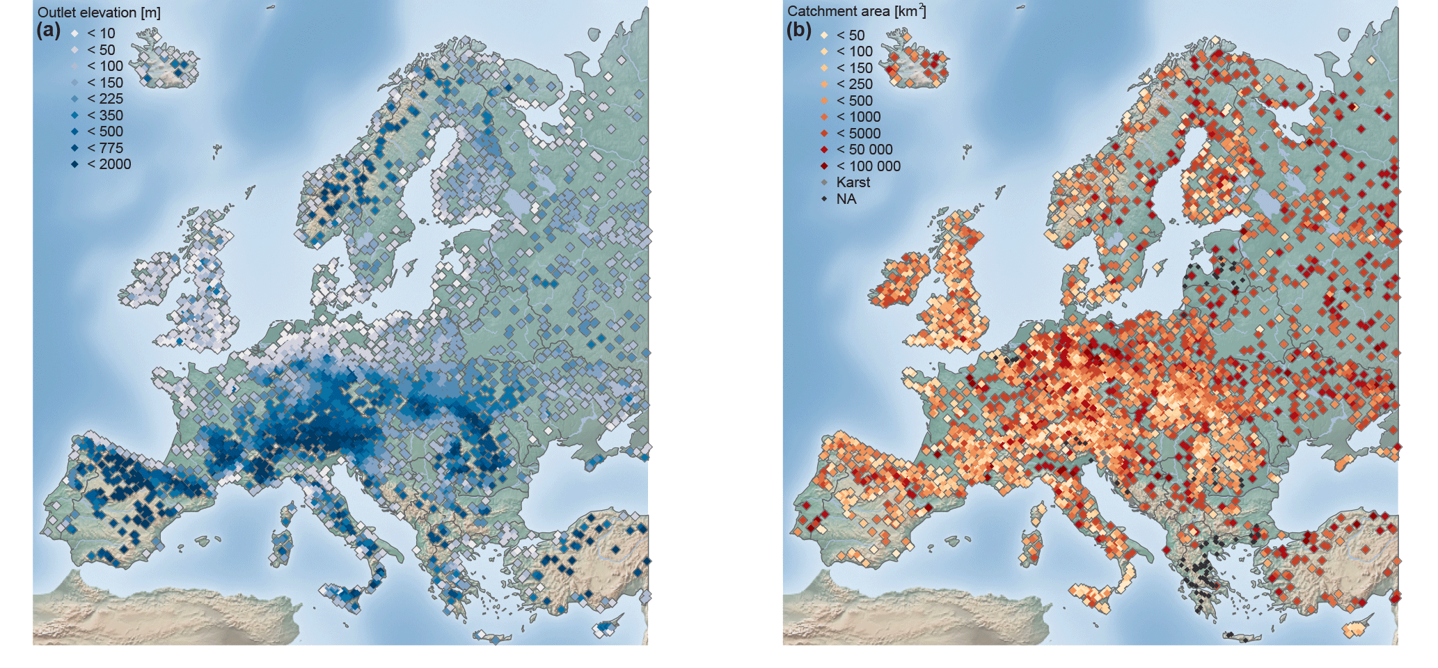
Figure 2Maps of station elevation at the catchment outlet (m) (a) and catchment area (km2) (b). In both panels, n= 4105 stations.
Catchments for which it was evident that the flood timing is strongly affected by known human modifications (e.g. dams or reservoirs) are excluded from the analysis. All catchments with more than 10 years of data within the period 1960–2010 were included in the first part of the analysis. In areas with high station density, such as Austria, Germany, and Switzerland, only stations with at least 49 years of data in the study period were included, to balance station density across Europe and to improve the visual representation on a European map. This selection resulted in 4105 hydrometric stations (Fig. 1) with station elevation ranging from −5.17 to 1961 m (Fig. 2a), catchment areas ranging from 10 to 100 000 km2 (Fig. 2b), and record lengths ranging from 11 to 51 years (Fig. 3). A total of 115 stations in the database have no catchment area assigned, either due to the existence of karst or missing metadata information. These stations are not shown in subsequent figures that display catchment area, which is indicated by a reduced number of stations in the respective figure caption.
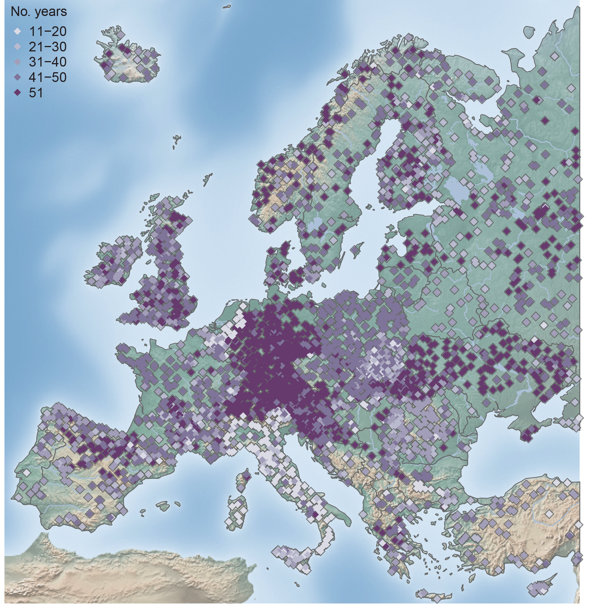
Figure 3Record length in number of years per station for the period 1960–2010, n= 4105 stations.
3.1 Flood seasonality
3.1.1 Mean flood seasonality and temporal flood concentration
The mean seasonality of annual maximum floods is determined using circular statistics (Bayliss and Jones, 1993; Mardia, 1972). In order to be able to calculate the mean date of flood occurrence (i.e. day of year, DOY) for a given station, the date of the flood occurrence Di (DOY) in year i is converted into an angular value θi in radians through
where Di= 1 corresponds to 1 January and Di=mi for 31 December, and where mi is the number of days in that year (365 or 366 for leap years). The mean date of flood occurrence at a station is then
with
where and are the cosine and sine components of the mean date, respectively, is the mean number of days per year (365.25), and n is the total number of flood peaks at that station during the study period.
In order to be able to interpret the mean flood seasonality, the concentration index R of the dates of AMF occurrence around the mean date is calculated. R can be interpreted as a measure of how well the flood seasonality is defined for a given catchment (Fig. 4b).
The concentration index R ranges from R= 0, representing no temporal concentration (i.e. floods are dispersed throughout the year and the seasonality vectors of the individual floods cancel out (reflective symmetry)), to R= 1, which indicates that all floods occur on the same day of the year.
There is a trade-off between good spatial coverage and the minimum record length needed for meaningful flood seasonality analysis. Based on simulated monthly flood frequencies from a uniform distribution, Cunderlik et al. (2004) recommend care when evaluating the results from records shorter than 30 years, because of the large sampling variability that might either artificially increase or mask the strength of the flood seasonality.
In the observational dataset analysed here, the mean values of the flood concentration index R change little with different record length from 11 to 51 years (±0.1 of the overall mean R value of 0.6, not shown). For the analyses of spatial patterns, priority is given to spatial coverage and therefore all 4105 stations (containing time series with a record length of 11–51 years) are used in the analysis of the mean seasonality, temporal flood concentration, and the cluster analysis. In the detailed analysis of the monthly flood characteristics only data with at least 30 years of record are used, as the above approximation of the confidence intervals is only valid for records with at least 30 data points (Sect. 3.3).
3.1.2 Circular uniformity
The spatial characteristics of flood seasonality can only be meaningfully interpreted if the data exhibit one or two preferred seasons in which floods occur (unimodal or bimodal flood seasonality). Therefore, stations for which the null hypothesis of circular uniformity (modified Kuiper's test, Mardia and Jupp, 2008) cannot be rejected (α= 0.1) are highlighted (i.e. 186 stations) and are further analysed for a possible connection with spatial location (Fig. 4b), catchment outlet elevation, and catchment area (Fig. 6). Only stations for which the null hypothesis of circular uniformity can be rejected are included in the remaining analyses (3919 stations), since one of the objectives of the paper is the identification of clusters with distinct flood seasonality characteristics.
3.2 Cluster analysis
A cluster analysis is conducted to identify regions with similar flood seasonality characteristics across Europe. Depending on the clustering method chosen, different regional clusters can emerge (Everitt et al., 2011). Here, the clusters are estimated using the k-means clustering algorithm; k-means can be considered superior to hierarchical clustering for the analysed dataset, as k-means clustering is less affected by outliers and can be applied to large datasets, preferably for sample sizes > 500 (Everitt et al., 2011). More information on the k-means clustering algorithm by Hartigan and Wong (1979) used in the calculation (the function “kmeans” is part of the R package “stats”) can be found in R-Core-Team (2017).
A total of 12 clustering variables are used, which contain the relative monthly frequency of flood occurrence for the months January to December. For each station, the monthly frequencies of the AMF are calculated. In order to reduce the influence of wide ranges between the variables used in the k-means clustering, a Z-score standardisation of the variables is performed (Vesanto, 2001). Here, the monthly flood frequencies of all stations are standardised to zero mean and a standard deviation of 1. The standardised monthly flood occurrences are the only input to the k-means clustering algorithm. Geographic location is not used as a clustering variable to allow for an independent evaluation of the clusters, based on the time of flood occurrence only. Clusters consisting of stations with close geographical proximity or similar catchment characteristics can therefore be considered more plausible than clusters for which this is not the case.
Selection of the number of clusters
One important step in clustering data is the decision on the number of clusters (k), as this number is not known a priori. In this study, different numbers of clusters are examined with the aim of obtaining homogenous groups (clusters) of stations that are as similar as possible (regarding the timing of flood occurrence) within their group but are also as dissimilar as possible from the stations not belonging to their group.
The performance of the k-means clustering algorithm is assessed using the silhouette value s(i) (Rousseeuw, 1987), which is a measure of how similar a station is to its own cluster compared to the other clusters. Silhouette values range from −1 (high similarity with the neighbouring cluster) to 1, with higher s(i) values indicating that the station has a high similarity to its own cluster.
For a number of k clusters (k > 1) the silhouette value s(i) can be calculated using Eq. (6),
where a(i) is the average dissimilarity of all variables (here the average Euclidean distance is used) of station i to all other stations in the same cluster (i.e. how distant the station is, on average, from the other stations) and b(i) is the average dissimilarity to all stations in the neighbouring cluster to station i (i.e. the cluster that has the lowest average dissimilarity from all other clusters). The mean silhouette value over a cluster ( thus indicates how similar, on average, the stations in a cluster are. The mean silhouette value over all stations in the dataset indicates how well the clustering algorithm has assigned the stations to their respective cluster. The number of k clusters that has both the highest and highest individual can be considered the best choice, i.e. the “optimal number” of clusters (Rousseeuw, 1987).
As a second criterion for the selection of k clusters, the “elbow method” based on the total sum of within-cluster sum of squares (TSSwithin) is used,
where k is the number of clusters, j is a specific cluster, and i is an individual station in that cluster, so that Yij is the ith observation in cluster j, and is the mean of Yij over the range of i.
With an increasing numbers of clusters k, the TSSwithin decreases. The optimal number of k clusters is determined using the magnitude of the reductions in the TSSwithin between two consecutive numbers of clusters. If the reductions do not decrease much beyond a certain number of k clusters, that number is considered a good choice. After accounting for the sensitivity of the initial centroid placements (see below), the final number of clusters is selected based on first the values and second the elbow method conditional on the TSSwithin values.
The k-means clustering algorithm is sensitive to the location of the initial k centroids to which the nearest neighbours are assigned (Steinley, 2003). This sensitivity affects both the selection of the “optimal number” of clusters k and the assignment of stations to a certain cluster. To account for this, the k-mean algorithm is at first repeated with 10 000 random centroid initialisations (seed vectors) and the initialisation with the highest mean silhouette value over all stations is then selected. As several initial centroid locations for k clusters can result in the same maximum value, all centroid initialisations that have the same maximum value are retained and further analysed with regard to their TSSwithin values.
From these initialisations, only the sets of initial centroids that have the same optimal number of clusters k based on the values and the evaluation of the TSSwithin values are retained as described above. As this can result in more than one set of initial centroids, the set that has the lowest TSSwithin of the remaining sets is chosen as the final location of the initial centroids.
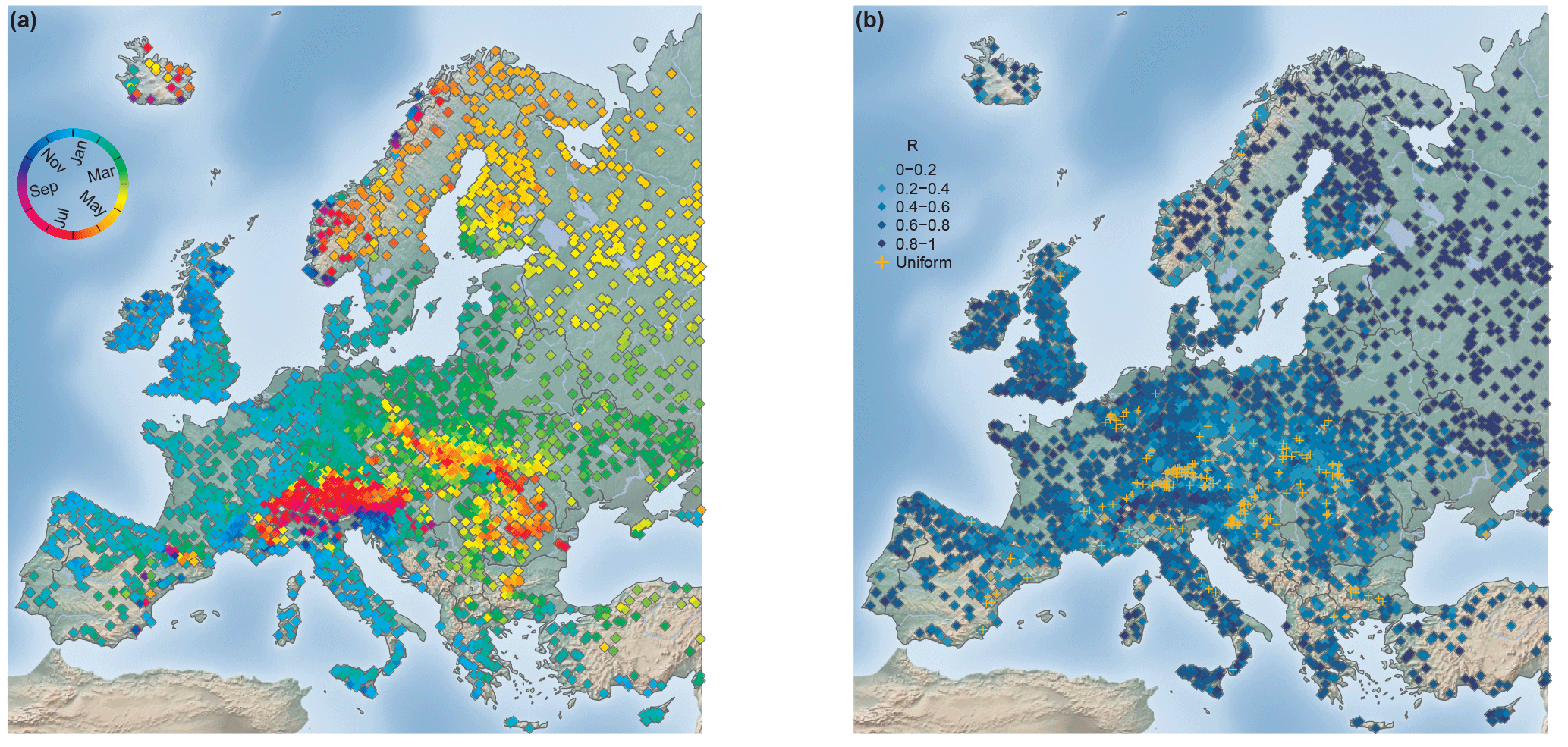
Figure 4Seasonality of floods in Europe for 1960–2010. Mean date of flood occurrence. (a) Flood concentration index R. (b) Stations for which circular uniformity could not be rejected (α= 0.1) (186 stations) are marked by orange crosses. In both panels, n= 4105 stations.
3.3 Analysis of temporal flood characteristics
3.3.1 Identification of flood-dominant and flood-scarce months
The k clusters obtained from the initialisation procedure described above are then further analysed for their temporal flood occurrence characteristics, with the aim of identifying months in which floods occurred often and months in which floods happen seldom or never (hereafter termed “flood-dominant” and “flood-scarce” months, respectively). This classification into flood-dominant and flood-scarce months is achieved by a significance test in which the observed monthly flood occurrence is compared to the expected occurrence of a uniform flood seasonality distribution (1∕12 of the floods are expected to occur in each month) (Cunderlik et al., 2004).
As the twelve months contain a different number of days, the monthly counts of flood occurrence ci need to be modified to match a “30-day month” to obtain adjusted monthly percentages of flood occurrences ( that allow a direct comparison of the counts. The term denotes the adjusted monthly count of flood occurrences with i being the months 1 to 12, and di the number of days in that month (February has 28.25 days to account for leap years).
The one-sided 95 % upper ( and lower ( confidence intervals are approximated following Cunderlik et al. (2004):
with n being here the record length.
If the monthly percentage of a given month is above or below the confidence interval, this month is considered to be either flood-dominant or flood-scarce respectively (at a 5 % significance level). Only stations with at least 30 years of data are analysed (3356 stations), as the approximation described above is only valid for records with at least 30 data points. The 563 stations with shorter records are excluded from the remaining analyses.
Depending on the record length, the upper and lower thresholds of the confidence interval vary. For example, for a 30-year-long record, the and for are 10.126 and 0.246 % of floods per month respectively (i.e. counts of flood occurrences for a given month of 3.037 and 0.073), whereas for a 51-year-long record the thresholds for are 15.251 and 2.629 % respectively (i.e. counts for a given month of 7.778 and 1.341). The months that have their within these two thresholds are not further classified and are labelled as “unclassified”. For each station independently, each month of the year is classified as flood-dominant, flood-scarce, or neither of them (i.e. unclassified), based on the individual thresholds determined based on the available record length.
3.3.2 Identification of bimodal and unimodal flood seasonality distributions
Flood-dominant or flood-scarce periods for a station are obtained by segmenting the year based on the consecutive occurrence of months with the same classification (i.e. either flood-dominant or flood-scarce). If the adjacent months at the beginning and the end of the year belong to the same classification, the months are combined to form one consecutive period. The length of the flood-dominant and flood-scarce periods is determined by summing the number of months within each individual period.
Additionally, based on the sequence of the two types of periods, the monthly flood seasonality distribution is identified as bimodal if two flood-dominant periods, independent of their length (i.e. a minimum of 1 month each), are separated by at least one flood-scarce month (before and after the flood-dominant). A unimodal flood seasonality distribution is identified if all flood-dominated months (minimum of 1 month) occur consecutively.
4.1 European flood seasonality characteristics
Figure 4 shows the mean flood seasonality and the temporal concentration of flood occurrence within the year. A distinct spatial pattern of the mean timing of floods within the year can be observed (Fig. 4a). Below 60∘ latitude, the mean seasonality transitions from winter floods in the west to spring floods in the east due to increasing continentality. Stations located in mountainous areas (e.g. the Alps, the Carpathians, and the Pyrenees) exhibit predominately summer floods and disrupt this west-to-east transition of mean flood timings. Above 60∘ latitude, spring floods dominate the spatial pattern, except for coastal areas in which autumn and winter floods are observed. The temporal concentration of floods around the mean date of flood occurrence (R value) (Fig. 4b) is highest in north-eastern Europe. High temporal concentration is also apparent at the western coast of Europe, except northern Europe, where floods are spread more evenly throughout the year. Catchments on the foothills of mountainous areas (e.g. around the Alps and the Carpathians) also tend to have smaller R values and sometimes exhibit a uniform occurrence of floods throughout the year. The orange crosses in Fig. 4b indicate the stations for which circular uniformity could not be rejected at a significance level of α= 0.1. The characteristics of stations with uniform flood occurrence are later examined in detail (see Fig. 6).
A complimentary procedure for examining the flood seasonality is the assessment of the frequency of floods occurring in the winter and summer half-years (Fig. 5). This assessment assists in the identification of regions in Europe with prolonged yet concentrated flood seasonality. For Europe, the winter and the summer half-years are defined for this procedure as October to March and April to September, respectively.
There is a clear dominance of summer floods in mountain ranges (e.g. Pyrenees, Alps, and Carpathians) and in the northern and north-eastern parts of Europe, which can be characterised by a continental climate. In the rest of Europe, floods predominately occur in the winter half-year. Transitional areas, for which no clear seasonal distinction can be made (< 60 % of either winter of summer half-year floods), can be found in and around Poland, Lithuania, Belarus, and parts of the Ukraine. In these transitional areas, no half-year flood season dominates, as the AMFs of these stations tend to occur in March and April around the cut off date separating the winter versus summer half-years. Additionally, a less well-defined flood seasonality can be found on the foothills of mountains, where both winter and summer floods occur (mixed distribution), depending on whether floods are snowmelt-induced, summer-rainfall-induced, or the floods are uniformly distributed throughout the year.

Figure 5Percentage of winter half-year (October to March) and summer half-year (April to September) floods. Dark purple or orange colours indicate dominance of the winter or summer half-year respectively; light colours indicate an almost equal occurrence in the two half-years; n= 4105 stations.
In order to examine further the relationship between uniform flood occurrence and week seasonality (low R values), the spatial location of the stations for which circular uniformity could not be rejected (at a significance level of α= 0.1) is shown in Fig. 4b. The stations with a uniform flood seasonality distribution are found predominately at low to medium-high altitudes (< 1000 m) (Fig. 6a) and in small catchments (Fig. 6b). However, for some of the stations with a small flood concentration index R, uniformity could not be rejected at a significance level of α= 0.1, which reveals that small R values do not necessarily indicate uniformity. These stations possess a skewed or a bimodal distribution of flood occurrence throughout the year.
For the European continent, stations with high elevation tend to have a high flood concentration index R and mainly occur in early summer (mean seasonality in May and June) (Fig. 6a). Uniformity in the seasonal flood occurrence was rejected for stations across all elevation levels. Only at lower elevations (< 1000 m), uniform distributions are observed. From Fig. 6b it is apparent that uniformity cannot be rejected for catchments of all sizes (note: 115 catchments with missing catchment area are not shown). Larger catchments tend to have a few stations with a flood concentration index < 0.2, most of which can be considered as having a uniform distribution, whereas catchments with less than 1000 km2 exhibit more often smaller R values and these tend to have uniform distributions (Fig. 6b). Generally, hydrological stations that have a small catchment area and a low catchment elevation are predominately found near the foothills of mountains. Therefore, uniformity of flood occurrence throughout the year seems to be predominately conditioned by geographical location, which corroborates the initial hypothesis obtained from mapped location shown in Fig. 2b.
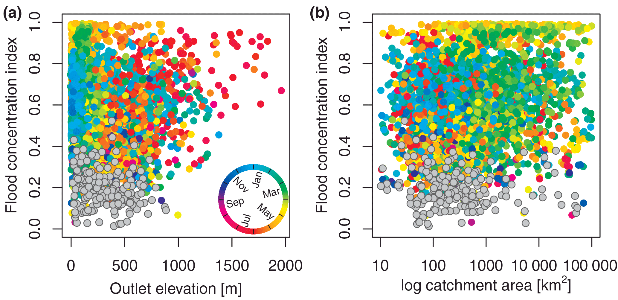
Figure 6Flood concentration index R of floods in Europe (1960–2010) dependent on station elevation (m a.s.l.), n= 4105 (a), and catchment area (km2), n= 3900. (b) Point colour indicates the mean timing of floods () derived for that station location. Grey points indicate the 186 stations for which circular uniformity could not be rejected (α= 0.1).

Figure 7Mean frequency of seasonal floods by ranges of outlet elevation (m a.s.l.), n= 3919 (a), and catchment area (km2), n= 3804 (b). In both panels, the ranges on the x axis were selected so that an approximately equal number of stations is allocated to each range. In both panels, stations with a uniform distribution are excluded.
The mean frequency of floods in each season (based on individual flood events) is shown in Fig. 7 (for all 3919 stations for which the null hypothesis of circular uniformity was rejected at α= 0.1). Floods occurring between January and March are classified here as winter floods, spring floods occur between April and June, summer floods occur between July and September, and autumn floods occur between October and December. Figure 7a displays an increase in the mean frequency of summer floods with increasing elevation and conversely a tendency towards decreases in the frequency of autumn and winter floods due to the increasing dominance of summer floods (see also Fig. 6a for the similarity with the mean flood seasonality). Autumn floods have the highest frequency in most of the elevation ranges analysed. In two elevation ranges (91 to 125 m and > 440 m), spring floods have the highest occurrence frequency. Combining these results with the ones obtained from Figs. 4 to 6, one can conclude that the high mean frequency of spring floods occurs either in catchments with intermediate elevation in north-eastern Europe or in, or around, mountainous areas (flood timing is often towards the end of June, close to July which is the first month used for the classification of summer floods).
Smaller catchments in Europe are more similar regarding their mean frequency of seasonal floods (Fig. 7b, note: 115 catchments with unknown catchment area are not shown). With increasing catchment area, the percentage of spring floods increases. This observed tendency is related to the uneven spatial distribution of larger catchments in the database (Fig. 2b). Stations with large catchment areas can be found predominately in central and eastern to north-eastern parts of Europe, which are dominated by spring floods.
Therefore, at European scale, catchment attributes such as catchment outlet elevation or catchment area alone cannot be considered as good indicators for flood seasonality. At large scale the geographical location is the most important part in determining the seasonal flood characteristics.

Figure 8Spatial distribution of the six clusters of monthly flood frequencies (a), n= 3919 stations. The vertical axes of the panel on the right shows the catchment outlet elevation (m a.s.l.) (b), n= 3804 stations.
4.2 Flood seasonality clusters
In the previous section, the strong influence of the geographical location on the timing of flood occurrence at a given station is apparent. Therefore, it is of interest to identify larger scale regions in Europe with relatively similar seasonal flood occurrence. These regions are identified based on the monthly frequencies of the AMF with the help of cluster analysis, after the best possible initial centroid locations are determined (see Sect. 3.2.1 for methodological details).
Table 1 summarises the sensitivity of the location of the initial centroids and shows the percentage of how often a specific number of clusters (5 7) obtained the highest mean silhouette value from the 10 000 random initial cluster centroids and the highest overall value. The results in Table 1 indicate that, with the same initial centroid placement for five, six, or seven clusters (same as five clusters plus one or two additional initial centroids for six and seven clusters respectively), 46 % of the random samples generated the highest values for k= 6 clusters. Additionally, the six initial cluster centroids result in clusters that obtain the maximum of 0.443 for all 10 000 random initialisations. In the initialisations for which five or seven clusters obtain the highest , the maximum are always lower than the maximum that is obtained with six clusters. Therefore, the sets of initial centroid locations that obtain the highest of all random initialisations (0.443) for k= 6 are chosen as candidates for further selection of the initial centroid position. From these only the sets of initial locations are retained, for which the elbow method (based on the reduction in the total within cluster sum of squares, TSSwithin) also results in k= 6 optimal clusters. As several sets with different initial centroid locations fulfil this criterion, the initial set of centroids that yields the lowest TSSwithin for k= 6 is selected and is used in the remainder of the study.
Table 1Number of clusters and average silhouette value for 10 000 random initial cluster centroids.

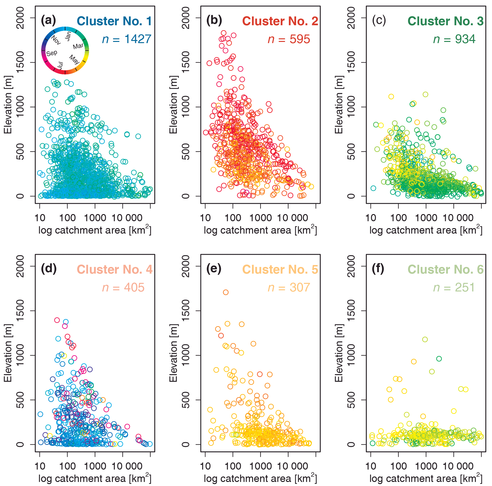
Figure 9Mean flood seasonality () as a function of catchment outlet elevation (m a.s.l.) and catchment area (km2) grouped by the six clusters. Colour of the points in all panels indicates the mean timing of floods at that hydrometric station. Total number of stations in the analysis is 3919; in each panel n denotes the number of stations assigned to a specific cluster (in panels a–f there are 115 stations (69, 4, 19, 14, 3, and 6 stations respectively) not being displayed due to unknown catchment area).
Spatial distribution and characteristics of flood seasonality clusters
Table 2The six clusters of monthly flood frequencies in Europe and their characteristics.
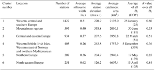
Figure 8 depicts the spatial distribution of the six clusters of monthly flood occurrences obtained using the methodology described above. Table 2 and Fig. 9 assist in interpreting of the clusters shown in Fig. 8.
Cluster 1 is located in western, central, and southern Europe and contains most of the stations (∼ 36 %). The mountainous regions in Europe (highest average outlet elevation), the Alps, and the Carpathian and Scandinavian mountains in Cluster 2 account for ∼ 15 % of the stations. Most stations, located in central and eastern Europe up to 55∘ N (∼ 24 %), are assigned to Cluster 3. Cluster 5 and 6, located predominately in northern and north-eastern Europe, are the two smallest clusters, containing ∼ 8 and ∼ 6 % of all stations respectively. Most of stations assigned to Cluster 6 are located above 60∘ N and are low-lying.
Clusters 1, 5, and 6 are well defined (i.e. high within-cluster similarity or average silhouette width . Cluster 4 is the least well-defined cluster in terms of and also in terms of spatial coherence. The stations in Cluster 4 are found in several regions of Europe (western British–Irish Isles, western coast of Norway, and northern Mediterranean). Cluster 4 has the smallest average catchment area and the highest spread of flood occurrence around the mean date of flood occurrence (early December) (see also “mean of all” in Fig. 10). The largest catchment areas are found in northern and north-eastern Europe (Cluster 3, 5, and 6). The average dates of the flood timing (Di) in Cluster 5 and Cluster 6 are mid-May and mid-April, respectively, with all floods being highly concentrated around the average date. Cluster 1 is also strongly seasonal with a mean flood occurrence in late January, whereas the mountainous areas (Cluster 2) have their mean flood occurrence in summer. Here Cluster 2 is considered to be spatially coherent, although the different mountainous areas are not necessary spatially connected to each other.
Overall, although the geographic location is not included as a variable for clustering, the location of a hydrometric station seems to be an important factor influencing flood seasonality and hence for determining the membership of a cluster. There are few stations that do not fit the large-scale, coherent cluster pattern (i.e. spatial outliers).

Figure 10Mean seasonality and temporal concentration of floods for each station (small points), the mean over all floods within specific clusters (large points), and the mean of all mean flood seasonalities (large points with crosses) within specific clusters. Colours correspond to clusters. Distance to centre is a measure of the temporal flood concentration index R, with the centre corresponding to R= 0, the black dashed circle to R= 0.5, and the outer full circle to R= 1. The grey dashed circles correspond to intervals of 0.1 R. Total number of stations: n= 3919.
Figure 10 shows the mean flood seasonality () for each station, the overall mean seasonality of all floods belonging to the same cluster, and the mean of all mean flood seasonalities, together with the respective temporal concentration around these means. The stations within their respective clusters display similar concentrations, as indicated by R values > 0.9 of the mean of the cluster mean flood seasonalities (large points with crosses). The exception is Cluster 4, which has the lowest temporal concentration of the mean floods, with R= 0.71. In this cluster, the temporal concentrations of the floods of the individual stations are lower than those of the stations in the other clusters. The R values of the mean of all AMFs (large points) in both Cluster 5 and Cluster 6 (R= 0.85 and R= 0.84, respectively) are close to the mean of all mean seasonalities. This indicates that, in these clusters, not only the mean seasonalities () but also the individual floods (Di) are temporally concentrated. The mean seasonalities of most of the stations assigned to these two clusters have a strong temporal concentration around their regional mean (high R value), and only a few stations have a larger spread around the mean date of flood occurrence. The R values of the regional mean seasonality of all AMF in the other clusters are much smaller than the R values of the mean of all mean seasonalities. This indicates that the clustering algorithm performs well with regard to clustering stations that have a similar mean seasonality, but individual flood events may exhibit higher temporal variability.
4.3 Temporal characteristics of individual flood seasonality clusters
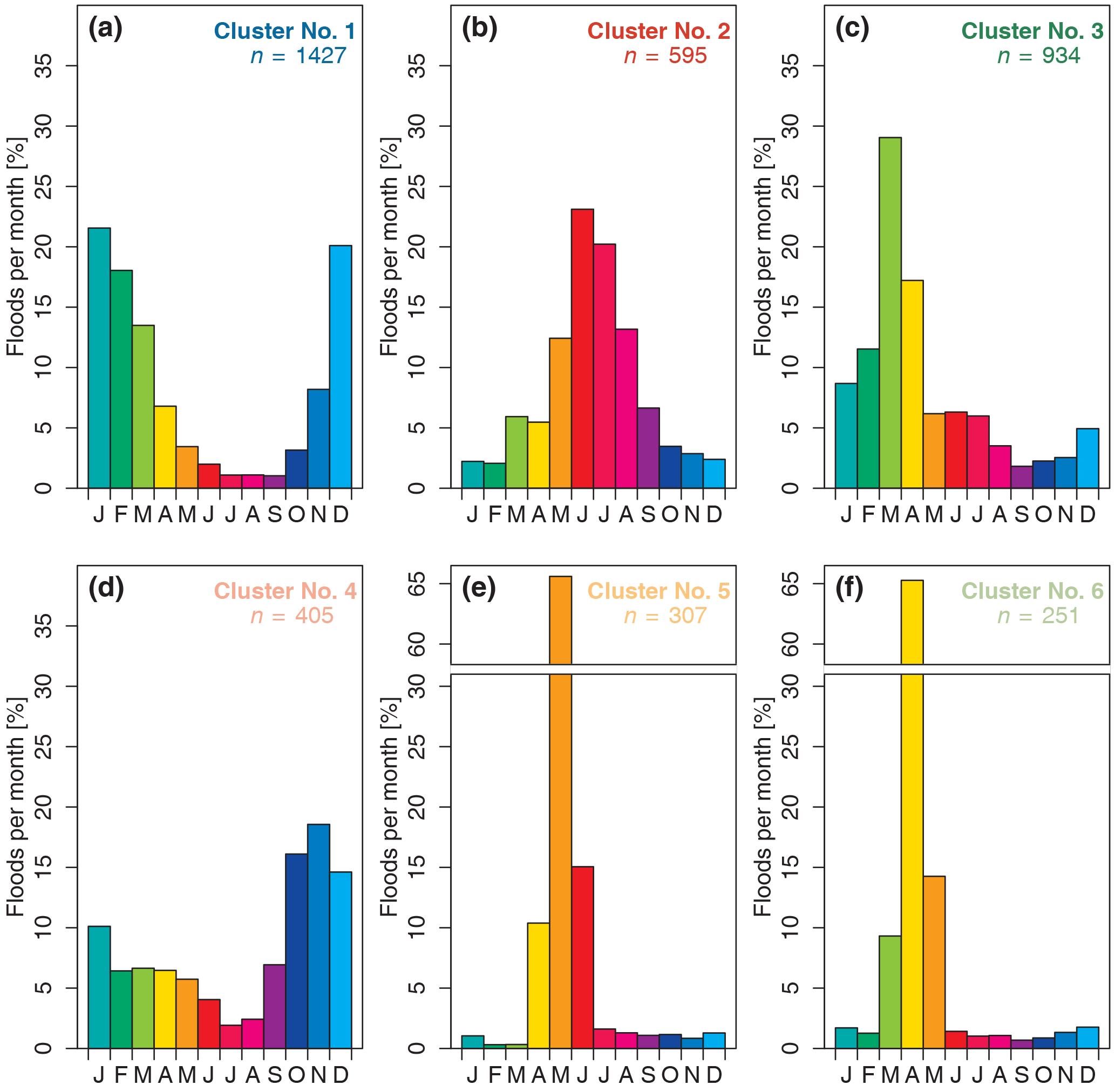
Figure 11Frequency of occurrence of maximum annual floods by month for the cluster centroids, CCs (i.e. cluster means). Total number of stations: n= 3919; in each panel n denotes the number of stations assigned to a specific cluster.
The mean flood seasonality for both stations and clusters has limited information content, as it only reflects the first moment of the seasonality distribution. Therefore, it is of interest to examine the full monthly flood distribution of each cluster. Theoretically, if all floods were equally spread over the year, each month would contain % of all the AMFs. Figure 11 shows the relative monthly frequency of AMFs of the cluster centroids (CCs) (i.e. the respective cluster means). All CCs have at least 1 month in which more than 18 % of the annual maximum floods occur. This indicates that in each of the CCs there is a dominant month in which floods tend to occur and therefore a distinct flood seasonality. The CCs of Cluster 5 and Cluster 6 in northern and north-eastern Europe have the most pronounced flood seasonality, where a single month (May and April, respectively) contains > 65 % of the AMFs. For both CCs the months before and after this peak account for ∼ 10 and ∼ 15 %, respectively, with the remaining months containing less than 3 % of the AMFs. CC 1 (western and southern Europe) and CC 2 (mountainous regions) exhibit an almost bell-shaped distribution, with the AMFs peaking in the winter and summer halves of the year, respectively. CC 3 (central and eastern Europe) peaks at the beginning of the year (strongest peak in March, 28 %), with less than 10 % if AMFs in the rest of the year. CC 4 is the cluster with the least pronounced peak in the monthly flood frequencies. There is a small peak of flood occurrences in the winter months (October to September, each month < 20 %) and a low flood season in the summer months.

Figure 12Box plot of the percentage of floods per month for each station, grouped by cluster (a–f). The top and bottom of the boxes show the 75th and 25th percentiles (i.e. the upper and lower quartiles) respectively, whiskers extend to 1.5× interquartile range beyond the box, the black band indicates the median, and outliers are shown as points. Total number of stations: n= 3919; in each panel n denotes the number of stations assigned to a specific cluster.
Figure 12 depicts the full range of relative monthly flood frequencies of all stations assigned to each cluster, to allow an in-depth interpretation of the results beyond the cluster mean (i.e. CC shown in Fig. 11). The shape of the monthly flood seasonality distribution of the medians of each cluster (i.e. monthly percentages) resembles the shape of the cluster centroids in Fig. 11 for most clusters. Differences in the shape of the seasonality distributions are mainly caused by individual stations that contain months with a frequency of AMFs deviating from the majority of the stations.
In Cluster 1, the shape of the distribution remains similar; however, for individual stations (outliers) the winter months have a much higher percentage of flood occurrences (up to 55 %), in the summer months the flood occurrences stay below 15 % of the AMF (Fig. 12a). In Cluster 2, June and July remain the months with the highest percentages. For some stations, August, and to a lesser extent May, are the most important months (Fig. 12b). This example shows the importance of not solely relying on the CC, as the aforementioned characteristic could not have been detected when examining the CC in Fig. 11b alone. October to February remain months with low flood occurrences even when a detailed station-based analysis for Cluster 2 is performed. Within Cluster 3, March and April stand out as the most important months of flooding, as it already seen in Fig. 11c. However, it becomes apparent now that these months have the highest spread between stations, while the other months have a much smaller spread (Fig. 12c). In Cluster 4, the CCs show frequent floods in October to January (Fig. 11d). However, when taking into account the full range of all the stations, the months April, May, and June also contain a high percentage of AMFs (up to 55 %) for individual stations (Fig. 12d). This characteristic is detectable in neither the CC nor the median of the cluster and indicates that, for some stations (i.e. locally), these months are very important in terms of flooding. The appearance of months with an additional secondary peak in flood occurrence indicates the possible existence of a bimodal distribution for several stations in Cluster 4. The medians and all individual stations of Cluster 5 and Cluster 6 exhibit a high occurrence of flooding in May and April, respectively, as was already indicated in Fig. 11. Most other months of the year show very low frequencies for the median with a very low spread between stations. The exceptions are the months immediately before and after the main flood month, which can have high percentages of flooding for individual stations as well (Fig. 12e and f). This high concentration of floods around a single month is the reason for the stations in Cluster 5 and 6 showing very high R values in Fig. 4b.
In summary, when taking all stations within a cluster into account, one can see that the main characteristics that are present in the monthly distributions of the CC are retained. However, some additional characteristics such as the emergence of a bimodal distribution in Cluster 4, which was smoothed-out in the CC or additional months with higher relative monthly flood frequencies and outliers, can be identified.
4.3.1 Flood-dominant and flood-scarce months
To further investigate the possible existence of a bimodal seasonality distribution, the classification into flood-dominant and flood-scarce months is performed, on records with more than 30 years of data (nsub) (see Sect. 3.3.1. for methodological details). Each cluster has more than 80 % of their stations with series longer than 30 years (see Table 3 for the exact numbers), and this ensures each cluster is still well represented in the following analysis.
Table 3Six clusters and their characteristic flood seasonality distributions, based on the subset of station with records > 30 years.
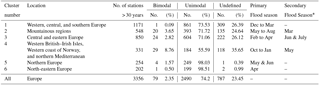
* Only for bimodal flood seasonality distributions in clusters with at least 20 stations.
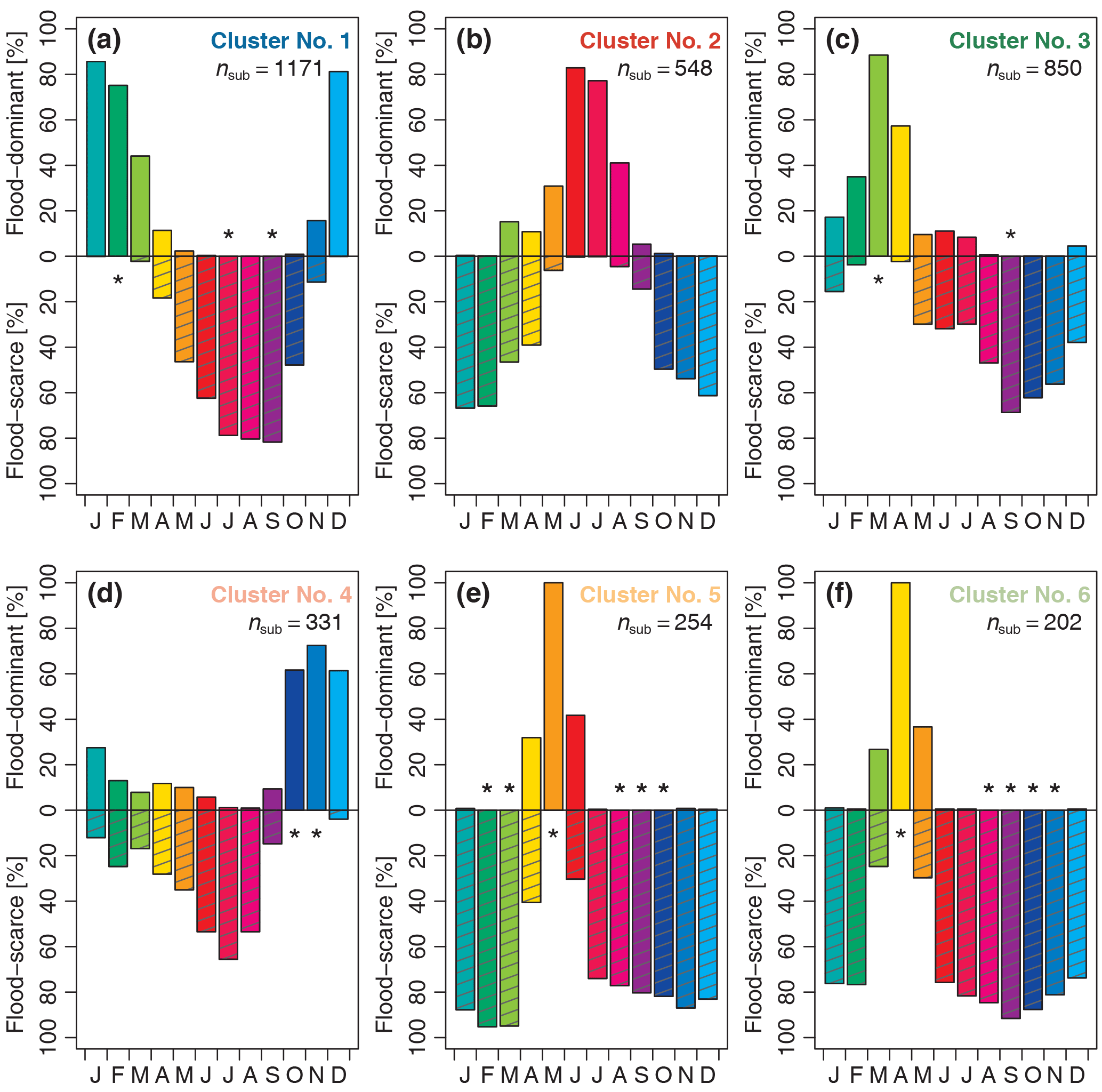
Figure 13Percentage of stations with months that can be considered significantly (α= 0.05) flood-dominant (upward bars) or flood-scarce (downward shaded bars) grouped by cluster (a–f). Months for which no station showed significance in the respective category are marked with a star. Total number of stations with records > 30 years: nsub= 3356. In each panel, nsub indicates the number of stations assigned to a specific cluster.
Figure 13 shows the percentages of stations in each cluster for which a specific month can be considered, as being flood-dominant or scarce (statistically significant at α= 0.05). In Cluster 5 and Cluster 6, the months May and April respectively are classified as flood-dominant for 100 % of the stations. There are four clusters with at least 1 month that can be considered not to be flood-dominated for 100 % of the station (marked by stars above the x axis in Fig. 13). In Cluster 1, this is the month June and September, in Cluster 3, September, in Cluster 5, February and March, and August to October and in Cluster 6, August to November. In all clusters, there is not a single month, for which all stations would exhibit flood scarcity (i.e. 100 %). Five out of six clusters (apart from Cluster 2) have at least 1 month that can be considered not to be flood-scarce for 100 % of the station (marked by stars below the x axis in Fig. 13). This is February for Cluster 1, March for Cluster 3, October and November for Cluster 4, and March and April for Cluster 5 and Cluster 6 respectively. Based on the percentage of stations that have flood dominance, there is again an indication in Cluster 4 that some of the stations might have a bimodal distribution with a primary peak in winter, and a secondary peak in April and May, with 12.01 and 10.21 % of the stations having a significant flood-dominated month respectively.
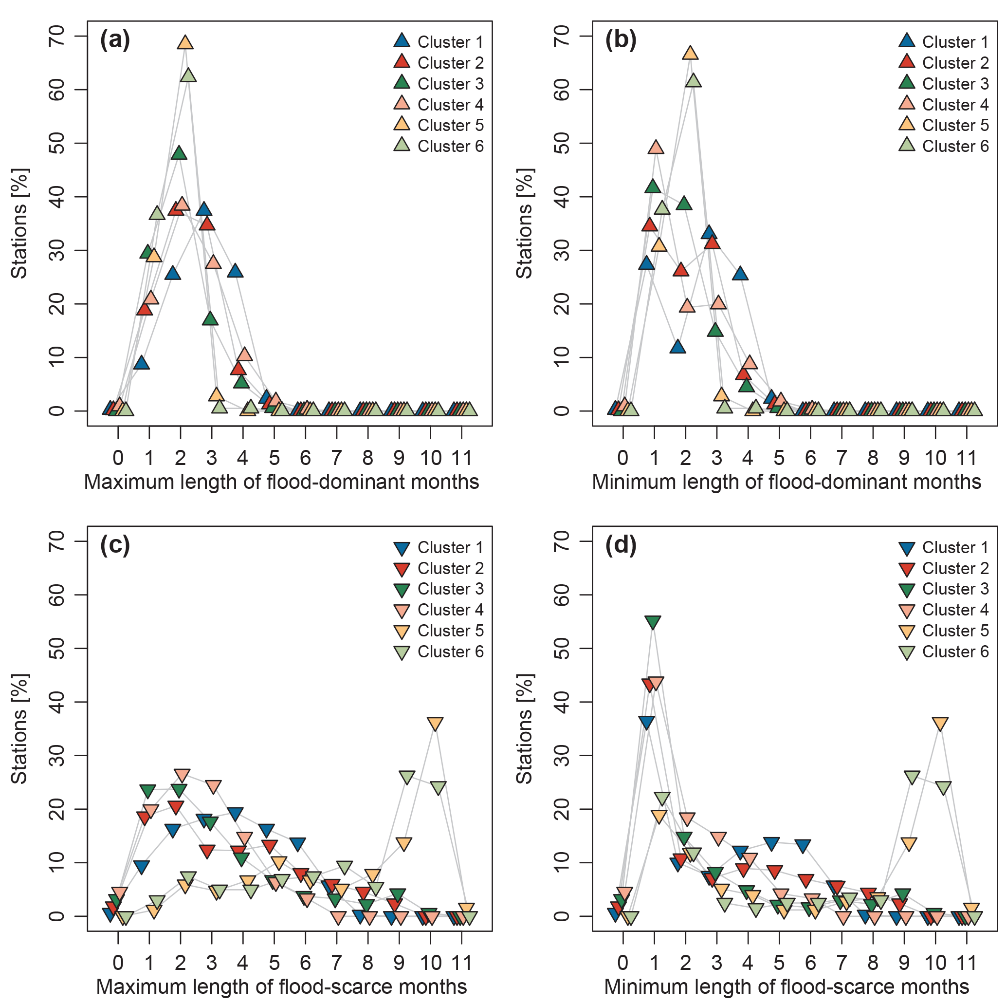
Figure 14Percentage of stations within the same consecutive monthly flood classification, grouped per cluster. The x axes show the maximum (a, c) and minimum number (b, d) of consecutive months classified as flood-dominant (a, b) and flood-scarce (c, d). Total number of stations with records > 30 years: nsub= 3356.
To obtain further insights into the temporal characteristics of the different flood periods, Fig. 14 shows the maximum and minimum duration (in months) for flood-dominant (a and b) and flood-scarce (c and d) periods respectively. In each panel, the percentages are plotted for each cluster separately.
There is a very small number of stations (< 1 %) in Clusters 1, 2, and 4 for which no significant flood-dominant season could be identified (i.e. 3, 2, and 2 stations, respectively) (Fig. 14a). This means that the floods are not uniformly distributed throughout the year (as stations for which uniformity could not be rejected were already removed from this dataset in a previous step), but the number of floods per month does not cross the threshold for the months to be classified as flood-dominant. All clusters contain stations that have a maximum of five consecutive flood-dominant months, with exception of Cluster 6, which has one station that has six consecutive months (Fig. 14a). Most of the stations have a maximum length of two consecutive months apart from Cluster 1, which has the highest number of stations with three consecutive months (Fig. 14a).
All stations in Clusters 5 and 6 have at least one flood-scarce month. In all other clusters, < 5 % of the stations have no flood-scarce month (Fig. 14c and d), i.e. most of the stations have a minimum duration of 1 flood-scarce month (Fig. 14d).
The existence of at least one flood-scarce month is of importance, as this is a necessary condition for the identification of bimodal flood seasonality distributions in the next part of the analysis. Most of the stations in Cluster 5 and 6 have the same maximum and minimum duration of 2 months when considering the flood-dominant months (Fig. 14a and b) and also the same number of maximum and minimum length of flood-scarce months between 9 and 10 months (Fig. 14c and d). This indicates that the seasonal flood seasonality distributions in these clusters are likely to be unimodal.
4.3.2 Classification of flood seasonality distributions
Based on the alternating occurrence of flood-dominant and flood-scarce months (see Sect. 3.3.2 for methodological details), the flood seasonality distributions of 79 stations are classified as bimodal. A total of 2490 stations have a unimodal seasonality distribution due to the uninterrupted occurrence of the flood-dominant months (Table 3).
Cluster 4 has the highest number of stations (29) and the highest percentage of stations (∼ 9 %) with bimodal distributions of all clusters. Cluster 4 has also the highest percentage of stations without a clearly defined flood seasonality distribution (∼ 36 % are undefined) and the lowest number of unimodal stations (∼ 56 %). This indicates that Cluster 4 is the cluster with the most diverse flood seasonality distributions, which is consistent with its low average silhouette values detected before and corroborates the results from the analysis steps performed before. In Cluster 2 and Cluster 3, 20 and 24 stations are classified as bimodal, and the other clusters contain less than 5 bimodal stations.
Primary and secondary flood seasons are identified, for each cluster separately, if the median of the monthly flood percentage is > 8.33 % (1∕12). Primary flood seasons are based on all stations with at least 30 years of data, and secondary flood seasons are identified from the bimodal flood seasonality distributions, from clusters with at least 5 bimodal stations (excluding the months that are already included in the primary flood season) (Table 3).
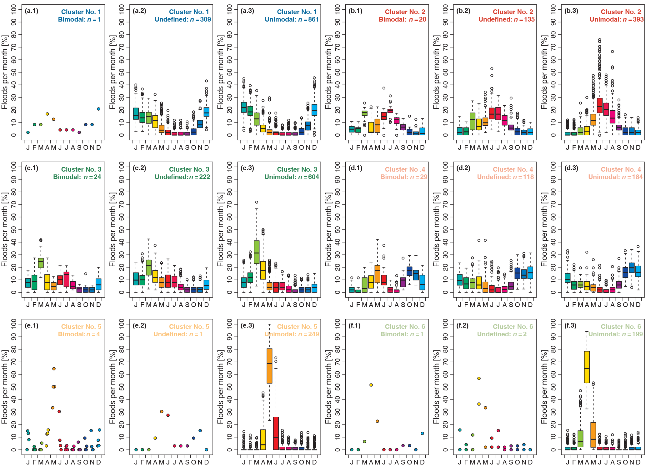
Figure 15Box plot of the percentage of floods per month for each station, of all stations with at least 30 years of data, grouped by their cluster (a–f) and by their annual flood seasonality distribution being bimodal, undefined, or unimodal (first, second, and third columns, respectively). The top and bottom of the boxes show the 75th and 25th percentiles (i.e. the upper and lower quartiles) respectively, whiskers extend to 1.5× interquartile range beyond the box, the black band indicates the median, and outliers are shown as points. Panels containing less than 5 stations show points instead of box plots. Number of stations: nsub= 3356; n denotes the number of stations within each flood distribution classification.
In Fig. 15, the monthly bimodal, unclassified, and unimodal flood seasonality distributions are shown for each cluster separately, to depict the differences between the different flood seasonality distributions in detail. In Cluster 1, 74 % of the stations have unimodal flood distributions and one station is classified as bimodal (Fig. 15a.3 and a.1 respectively). The other stations in Cluster 1 have an unclassified seasonality distribution (Fig. 15a.2), which is mainly due to the absence of an additional month classified as either flood-dominant or flood-scarce. Cluster 2, Cluster 3, and Cluster 4 show a monthly seasonality distribution with a distinct secondary flood season (Fig. 15b.1 to d.1). In the mountainous regions (Cluster 2), the secondary peak in the bimodal flood seasonality distribution in March precedes the main flood season in summer. In central and eastern Europe (Cluster 3) the main flood season in February to April is followed by secondary flooding in June and July (influence of summer rainfall events). In Cluster 4, the primary flood season in October to January is followed by an additional month of flooding in May. A total of 98 % of the stations in Cluster 5 and Cluster 6 in northern and north-eastern Europe are classified as unimodal (Fig. 15e.3 to f.3 respectively).
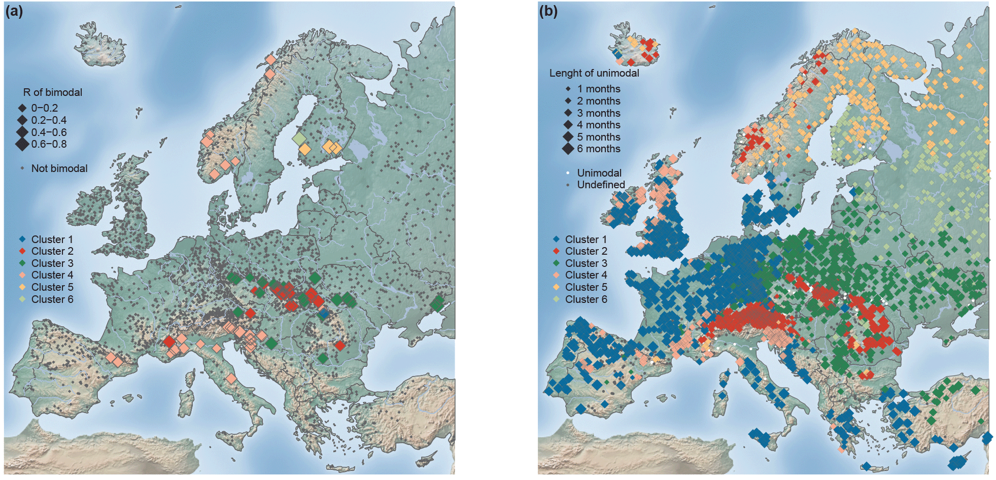
Figure 16Spatial distribution of the stations with bimodal flood seasonality distributions (n= 79) with the point size scaled by concentration R (a), and stations with unimodal distributions (n= 2490) with the point size scaled by the length of the flood-dominant period (b).
4.3.3 Spatial distribution of bimodal and unimodal flood seasonality distributions
Figure 16 shows the spatial pattern and flood seasonality characteristics of the stations with a clear bimodal or unimodal flood seasonality distribution for each cluster separately.
For most of the stations that exhibit a bimodal seasonality distribution, the R value is low (mean R value of all bimodal stations is 0.35) (Fig. 16a). However, bimodality does not necessarily imply a low concentration around the mean. If, for instance, the two flood seasons are separated by only one flood-scarce month, the R value can be high even in the case of bimodality. The station with the highest R value of all bimodal stations (R= 0.73) is located in Finland (Cluster 5), for which the secondary flood season occurs just 2 months before the primary flood season. Even though bimodality in the flood seasonality distribution is only detected in a small number of stations, the locations of these stations are not randomly distributed across Europe, but rather located in close spatial proximity to each other in spatially distinct regions.
Unimodal flood seasonality can be found in all regions across Europe (Fig. 16b). In northern and eastern Europe (Cluster 5 and Cluster 6), the duration of the period of flood-dominant months (unimodal seasonality distribution) is the shortest found among all clusters, and lasts on average 1.73 and 1.65 months, respectively. The stations in Cluster 1 have, on average the longest duration (∼ 3.2 months). In Cluster 2, Cluster 3, and Cluster 4 the periods of unimodal flood-dominant months last, on average 2.57, 2.16, and 2.65 months respectively.
This study provides a detailed analysis of the seasonality characteristics of annual maximum floods in Europe. While previous studies analysed the mean flood seasonality at national or regional scale, this paper aims to identify large-scale geographical regions with similar temporal flood characteristics and describe the flood seasonality of these regions in detail.
From the results obtained one can conclude that in Europe the station elevation (i.e. the catchment outlet elevation) or the catchment area explains the timing of the flood occurrence to a lesser degree than geographical location. Previous studies (e.g. Lecce, 2000, in the US) have suggested that catchment area has a strong effect on the flood seasonality (higher flood frequency in summer and autumn due to short-duration summer storms of limited areal coverage in small catchments, i.e. < 100 km2). In Europe, this does not seem to be the case. Smaller catchments show little difference in their flood seasonality when compared to larger catchments. Here a noticeable change with catchment area is only apparent in spring floods, which have a higher frequency in larger catchments. This increase in spring floods with larger catchment area is likely linked to the uneven spatial distribution of larger catchments, which are predominately found in eastern Europe, where a continental climate is dominant. Therefore, in Europe the observed changes of seasonal floods cannot be linked to catchment area alone due to the existence of a spatially coherent west-to-east transition from winter to spring floods across Europe.
It would have been interesting to investigate if the catchment mean or maximum elevation would correlate better with the observed flood seasonality patterns and clusters compared to the catchment outlet elevation used here; however, this information was only available for few of the stations and could be analysed in future if such information becomes available.
To obtain homogenous regions with distinct flood seasonalities, the clustering was performed on the monthly frequency of the annual maximum flood occurrence. Even without using the geographical location as a variable in the clustering, spatially coherent larger-scale clusters emerged that displayed distinct characteristics with regard to their flood seasonality distributions. The spatial seasonality patterns detected are similar to those found in smaller scale studies (some of which used different methods). For example, the clusters detected in this study had similar spatial boundaries to the three clusters identified by Beurton and Thieken (2009) in Germany. Cunderlik et al. (2004) detected three regions with different flood seasonality in Great Britain, whereas this study identified two clusters. Their region with a high number of floods in November (flood type 1) corresponds approximately to Cluster 4 identified in this study and their flood type 3 (floods occurring on average in January) corresponds to Cluster 1. They considered flood type 2 a transitional type between type 1 and type 3, which is included in Cluster 1 of this study due to the similarity of monthly AMF frequencies. Overall, differences between local scale and continental scale analyses can be expected, as the differences in the monthly flood frequencies that appear to be important at a smaller scale may be of lesser importance at a larger scale. Larger differences in the monthly flood seasonality distributions are observed across Europe due to the existence of a larger variety of flood generation processes.
Based on the mean flood seasonality, the temporal concentration of the AMF around the mean timing, and the geographical location on the map, one can hypothesise the causes behind the observed patterns. For example, Cluster 5 and Cluster 6 in eastern and north-eastern Europe are likely to be predominately driven by snowmelt processes (see also Blöschl et al., 2017), which result in a high temporal concentration within a month due to the relatively fast melting of the snow once the temperatures rise in the spring. Compared to Cluster 5 and Cluster 6, Cluster 3 is located further to the south and further to the west. These locations are marked by earlier snowmelt and a stronger maritime influence, which cause the floods in Cluster 3 to occur earlier in the year and exhibit a stronger influence of winter precipitation. For Cluster 2, which is primarily located in and around mountainous regions, one can infer that the AMFs are caused by both snowmelt and glacier melt in the summer, and by heavy precipitation occurring in the summer months. For the coastal stations located in Cluster 1, with strong maritime influence, station elevation has little influence on the temporal occurrence of the annual maximum floods, as snow accumulation and snowmelt are scarce. Therefore, the floods in this cluster can be considered to be mainly driven by extreme precipitation in late winter and early spring (see also Blöschl et al., 2017).
Cluster 4 is the most geographically dispersed cluster of all. The stations of Cluster 4 are located at the western coast of the British–Irish Isles, the western coast of Norway, and the northern coasts of the Mediterranean. The temporal distribution of the AMFs within the year shows a bimodal distribution for almost 9 % of the stations in this cluster. The floods can be considered to be predominately driven by late autumn and early winter precipitation (primary flood season), but also contain some floods caused by spring and early summer precipitation (secondary flood season).
In this study, only the annual maximum floods were available, but if more than one large flood event per year would be analysed (e.g. using partial duration series) the number of stations with bimodal distributions would probably be higher, as secondary flood maxima occurring in a year would also be included. The differences in the flood seasonality characteristics between using annual maxima or multiple peak events per year should be investigated as soon as appropriate data for such an analysis become available at a European scale.
Nevertheless, the detailed spatial and temporal flood seasonality information obtained in this study is important for practical applications, particularly for regions in which only limited information exists so far. Such applications include but are not limited to farming operations, fluvial ecosystem management, water management (reservoirs and dams), hydropower production, flood protection policy, and regional flood frequency analysis (see for example Barnett et al., 2005; Blöschl et al., 2017; Klaus et al., 2016; Köplin et al., 2014; Ryberg et al., 2016). Additionally, knowledge of the existence of these large-scale flood seasonality characteristics provides an important baseline for future research on floods in Europe. For example, the flood seasonality patterns can be used as an additional metric to test large-scale hydrological models for their ability to reproduce the spatial and temporal flood characteristics.
Moreover, the detailed assessment based on monthly flood occurrence, along with the identification of the spatial patterns of uniform, unimodal, and bimodal flood seasons, provides a starting point to assess the existence of one dominant or multiple flood-generating processes for distinct regions in Europe. For example, if the monthly flood seasonality distribution consists of a single peak change that ranges over just a few months (similar to Cluster 5 and Cluster 6), then it is likely that the floods are generated by one temporally distinct driving process, such as snowmelt. However, if the temporal flood seasonality distribution is spread over several months it is likely that several drivers (rain, rain on snow, snowmelt, or soil moisture) tend to cause floods. Mixed flood drivers seem to be involved in shaping the flood seasonality in Cluster 4, which contains stations that are located at the eastern coast of the British–Irish Isles and the northern Mediterranean coast, which have a different Köppen–Geiger climate classification, but yet a similar flood seasonality distribution.
Overall, the existence of a large-scale pattern of flood seasonality characteristics points to climate being the dominant large-scale control, with local catchment characteristics modulating the climatic inputs. Given the variety of flood generation processes across Europe and their distinct local interplay, the detailed attribution of the detected large-scale pattern to specific climate characteristics and weather patterns is beyond the scope of this study and merits a follow-up study.
The assessment presented here summarises the temporal flood seasonality distributions and the spatial patterns over the period 1960–2010. The timing of floods within this period, however, varies and changes in the flood seasonality distribution have been linked to a changing climate. For example, shifts in the timing of floods have been observed (e.g. Arheimer and Lindström, 2015; Blöschl et al., 2017; Wilson et al., 2010). For example, the timing of snowmelt-generated floods has shifted towards earlier in the season as a result of earlier snowmelt due to rising temperatures. This shift is projected to continue for as long as snowmelt is relevant for flooding (e.g. Teutschbein et al., 2015 for Swedish catchments).
If snow processes become less important due to higher temperatures in the distant future, flood seasonality patterns in north-eastern Europe may change completely if other flood generation processes may become dominant. In Europe, more research is needed to determine how the spatial and temporal clusters of flood seasonality might change in future, due to the complexity of the flood generation processes (precipitation occurrence and temperature, and soil moisture), their interactions, and also their interactions with the physical catchment properties (Stewart, 2009). If raising temperatures in the future result in diminished snow accumulation during winter, the annual maximum flood caused by spring snowmelt might be replaced by an annual maximum flood caused by increased precipitation depending on the season in which the rainfall occurs. The effect of increasing temperatures leading to earlier floods could also be masked by a concurrent precipitation increase in the cold season, resulting in higher snow accumulation and delayed melt (Kay and Crooks, 2014), causing the floods to occur later.
Due to differences in the flood generation processes and how they are captured by hydrological models, future projections of flooding diverge. This is particularly the case for floods generated by high-intensity precipitation, which is difficult to project into the future (Kundzewicz et al., 2017). Additionally, not only the amount of precipitation determines flood generation, but also the spatio-temporal distribution and the antecedent soil moisture conditions, which will also affect the flood seasonality projects. Given the aforementioned future uncertainties together with the absence of a detailed study on the flood-generating processes across Europe, it is currently elusive to formulate a hypothesis of how the spatial and temporal clusters of flood seasonality observed in the current study period may evolve in future.
This study identifies spatially distinct regions with characteristic patterns of temporal flood occurrence. A transition in the pattern of mean seasonality is apparent, from winter floods in western Europe to late spring and early summer floods in eastern Europe, onto which (depending on the region) late spring to summer floods are superimposed.
The temporal concentration of floods around the mean date of flood occurrence is highest in north and north-eastern Europe and on the western lower latitude coasts. This is also apparent in the low temporal spread of floods (on average less than 2 months) and the high occurrence of stations with a unimodal flood season in these regions.
The occurrence of a bimodal flood seasonality distribution over the year is only detected in a small number of stations. Therefore, bimodality in the temporal distribution of annual maximum floods can be considered a local phenomenon, occurring in spatially distinct locations in Europe. Nevertheless, in these regions (predominately mountain foothills) the existence of a distinct secondary flood season is of practical importance, for example for reservoir and flood risk management.
Overall, the results suggest that for most of the stations geographical location and hence regional climate is the most important factor influencing the timing of annual maximum floods in Europe. Therefore, the study can be considered a contribution towards advancing the understanding of geographical and climate sensitivity of annual maximum floods and their temporal characteristics across Europe. Given the strong spatial consistency of the clusters obtained, the results of this study will also be important for an improved understanding of flood generation mechanisms at the European scale and the new insights on the flood seasonality characteristics can for example provide a benchmark for the assessment of Europe-wide hydrological model output.
The data analysed in this study is based on the database from the works of Hall et al. (2015) and Blöschl et al. (2017) with additional some updates.
The supplement related to this article is available online at: https://doi.org/10.5194/hess-22-3883-2018-supplement.
The authors declare that they have no conflict of interest.
The research was supported by the ERC Advanced Grant “FloodChange”
Project No. 291152.
All calculations and figures were produced using R (R-Core-Team, 2017). The
following packages used in the study are acknowledged: “classInt”,
“cluster”, “fpc”, “maptools”, “plot3D”, “plotrix”, “plyr”, “raster”,
“RColorBrewer”, “rgdal”, and “rworldmap”. The authors would like to
acknowledge relevant discussions with Rui Perdigão and thank all data
providers and fellow researchers involved in the data preparation.
Edited by: Giuliano Di Baldassarre
Reviewed by: Korbinian Breinl and one anonymous referee
Arheimer, B. and Lindström, G.: Climate impact on floods: changes in high flows in Sweden in the past and the future (1911–2100), Hydrol. Earth Syst. Sci., 19, 771–784, https://doi.org/10.5194/hess-19-771-2015, 2015.
Barnett, T. P., Adam, J. C., and Lettenmaier, D. P.: Potential impacts of a warming climate on water availability in snow-dominated regions, Nature, 438, 303–309, 2005.
Bayliss, A. C. and Jones, R. C.: Peaks-over-threshold flood database: Summary statistics and seasonality, IH Report No. 121, Institute of Hydrology, Wallingford, UK, 1993.
Beurton, S. and Thieken, A. H.: Seasonality of floods in Germany, Hydrolog. Sci. J., 54, 62–76, https://doi.org/10.1623/hysj.54.1.62, 2009.
Blöschl, G., Hall, J., Parajka, J., Perdigão, R. A. P., Merz, B., Arheimer, B., Aronica, G. T., Bilibashi, A., Bonacci, O., Borga, M., Čanjevac, I., Castellarin, A., Chirico, G. B., Claps, P., Fiala, K., Frolova, N., Gorbachova, L., Gül, A., Hannaford, J., Harrigan, S., Kireeva, M., Kiss, A., Kjeldsen, T. R., Kohnová, S., Koskela, J. J., Ledvinka, O., Macdonald, N., Mavrova-Guirguinova, M., Mediero, L., Merz, R., Molnar, P., Montanari, A., Murphy, C., Osuch, M., Ovcharuk, V., Radevski, I., Rogger, M., Salinas, J. L., Sauquet, E., Šraj, M., Szolgay, J., Viglione, A., Volpi, E., Wilson, D., Zaimi, K., and Živković, N.: Changing climate shifts timing of European floods, Science, 357, 588–590, https://doi.org/10.1126/science.aan2506, 2017.
Cunderlik, J. M., Ouarda, T. B., and Bobée, B.: On the objective identification of flood seasons, Water Resour. Res., 40, W01520, https://doi.org/10.1029/2003WR002295, 2004.
Everitt, B. S., Landau, S., Leese, M., and Stahl, D.: Cluster Analysis, Wiley Online Library, 2011.
Garner, G., Van Loon, A. F., Prudhomme, C., and Hannah, D. M.: Hydroclimatology of extreme river flows, Freshwater Biol., 60, 2461–2476, https://doi.org/10.1111/fwb.12667, 2015.
Hall, J., Arheimer, B., Borga, M., Brázdil, R., Claps, P., Kiss, A., Kjeldsen, T. R., Kriauciuniene, J., Kundzewicz, Z. W., Lang, M., Llasat, M. C., Macdonald, N., McIntyre, N., Mediero, L., Merz, B., Merz, R., Molnar, P., Montanari, A., Neuhold, C., Parajka, J., Perdigão, R. A. P., Plavcová, L., Rogger, M., Salinas, J. L., Sauquet, E., Schär, C., Szolgay, J., Viglione, A., and Blöschl, G.: Understanding flood regime changes in Europe: a state-of-the-art assessment, Hydrol. Earth Syst. Sci., 18, 2735–2772, https://doi.org/10.5194/hess-18-2735-2014, 2014.
Hall, J., Arheimer, B., Aronica, G. T., Bilibashi, A., Bohác, M., Bonacci, O., Borga, M., Burlando, P., Castellarin, A., Chirico, G. B., Claps, P., Fiala, K., Gaál, L., Gorbachova, L., Gül, A., Hannaford, J., Kiss, A., Kjeldsen, T., Kohnová, S., Koskela, J. J., Macdonald, N., Mavrova-Guirguinova, M., Ledvinka, O., Mediero, L., Merz, B., Merz, R., Molnar, P., Montanari, A., Osuch, M., Parajka, J., Perdigão, R. A. P., Radevski, I., Renard, B., Rogger, M., Salinas, J. L., Sauquet, E., Šraj, M., Szolgay, J., Viglione, A., Volpi, E., Wilson, D., Zaimi, K., and Blöschl, G.: A European Flood Database: facilitating comprehensive flood research beyond administrative boundaries, Proc. IAHS, 370, 89–95, https://doi.org/10.5194/piahs-370-89-2015, 2015.
Hartigan, J. A. and Wong, M. A.: Algorithm AS 136: A k-means clustering algorithm, J. Roy. Stat. Soc. C-App., 28, 100–108, https://doi.org/10.2307/2346830, 1979.
Jeneiová, K., Kohnová, S., Hall, J., and Parajka, J.: Variability of seasonal floods in the Upper Danube River basin, J. Hydrol. Hydromech., 64, 357–366, https://doi.org/10.1515/johh-2016-0037, 2016.
Kay, A. and Crooks, S.: An investigation of the effect of transient climate change on snowmelt, flood frequency and timing in northern Britain, Int. J. Climatol., 34, 3368–3381, https://doi.org/10.1002/joc.3913, 2014.
Klaus, S., Kreibich, H., Merz, B., Kuhlmann, B., and Schröter, K.: Large-scale, seasonal flood risk analysis for agricultural crops in Germany, Environ. Earth Sci., 75, 1–13, https://doi.org/10.1007/s12665-016-6096-1, 2016.
Köplin, N., Schädler, B., Viviroli, D., and Weingartner, R.: Seasonality and magnitude of floods in Switzerland under future climate change, Hydrol. Process., 28, 2567–2578, https://doi.org/10.1002/hyp.9757, 2014.
Kundzewicz, Z., Krysanova, V., Dankers, R., Hirabayashi, Y., Kanae, S., Hattermann, F., Huang, S., Milly, P., Stoffel, M., Driessen, P., Matczak, P., Quevauviller, P., and Schellnhuber, H.-J.: Differences in flood hazard projections in Europe-their causes and consequences for decision making, Hydrolog. Sci. J., 62, 1–14, 2017.
Lecce, S.: Spatial variations in the timing of annual floods in the southeastern United States, J. Hydrol., 235, 151–169, https://doi.org/10.1016/S0022-1694(00)00273-0, 2000.
Mardia, K. V.: Statistics of directional data, Academic Press Inc. London., 1972.
Mardia, K. V. and Jupp, P. E.: Tests of Uniformity and Tests of Goodness-of-Fit, in Directional Statistics, John Wiley & Sons, Inc., 93–118, 2008.
Mediero, L., Kjeldsen, T., Macdonald, N., Kohnová, S., Merz, B., Vorogushyn, S., Wilson, D., Alburquerque, T., Blöschl, G., Bogdanowicz, E., Castellarin, A., Hall, J., Kobold, M., Kriauciuniene, J., Lang, M., Madsen, H., Gül, G. O., Perdigão, R. A. P., Roald, L. A., Salinas, J. L., Toumazis, A. D., Veijalainen, N., and Þórarinsson, Ó.: Identification of coherent flood regions across Europe by using the longest streamflow records, J. Hydrol., 528, 341–360, https://doi.org/10.1016/j.jhydrol.2015.06.016, 2015.
Parajka, J., Kohnová, S., Merz, R., Szolgay, J., Hlavcová, K., and Blöschl, G.: Comparative analysis of the seasonality of hydrological characteristics in Slovakia and Austria, Hydrolog. Sci. J., 54, 456–473, https://doi.org/10.1623/hysj.54.3.456, 2009.
R-Core-Team: R – A Language and Environment for Statistical Computing, Vienna, Austria, available at: https://www.R-project.org/, last access: 28 September 2017.
Rousseeuw, P. J.: Silhouettes: A graphical aid to the interpretation and validation of cluster analysis, J. Comput. Appl. Math., 20, 53–65, https://doi.org/10.1016/0377-0427(87)90125-7, 1987.
Ryberg, K. R., Akyüz, F. A., Wiche, G. J., and Lin, W.: Changes in seasonality and timing of peak streamflow in snow and semi-arid climates of the north-central United States, 1910–2012, Hydrol. Process., 30, 1208–1218, https://doi.org/10.1002/hyp.10693, 2016.
Steinley, D.: Local optima in K-means clustering: what you don't know may hurt you, Psychol. Methods, 8, 294–304, https://doi.org/10.1037/1082-989X.8.3.294, 2003.
Stewart, I. T.: Changes in snowpack and snowmelt runoff for key mountain regions, Hydrol. Process., 23, 78–94, https://doi.org/10.1002/hyp.7128, 2009.
Teutschbein, C., Grabs, T., Karlsen, R. H., Laudon, H., and Bishop, K.: Hydrological response to changing climate conditions: Spatial streamflow variability in the boreal region, Water Resour. Res., 51, 9425–9446, https://doi.org/10.1002/2015WR017337, 2015.
Vesanto, J.: Importance of Individual Variables in the k-Means Algorithm, in: Advances in Knowledge Discovery and Data Mining: 5th Pacific-Asia Conference, PAKDD 2001 Hong Kong, China, 16–18 April 2001, Proceedings, edited by: Cheung, D., Williams, G. J., and Li, Q., Springer, Berlin, Heidelberg, 513–518, 2001.
Wilson, D., Hisdal, H., and Lawrence, D.: Has streamflow changed in the Nordic countries? – Recent trends and comparisons to hydrological projections, J. Hydrol., 394, 334–346, 2010.
Ye, S., Li, H.-Y., Leung, L. R., Guo, J., Ran, Q., Demissie, Y., and Sivapalan, M.: Understanding flood seasonality and its temporal shifts within the contiguous United States, J. Hydrometeorol., 18, 1997–2009, https://doi.org/10.1175/JHM-D-16-0207.1, 2017.