the Creative Commons Attribution 4.0 License.
the Creative Commons Attribution 4.0 License.
 | 22 May 2018
A spatially detailed blue water footprint of the United States economy
Richard R. Rushforth
Benjamin L. Ruddell
This paper quantifies and maps a spatially detailed and economically complete blue water footprint for the United States, utilizing the National Water Economy Database version 1.1 (NWED). NWED utilizes multiple mesoscale (county-level) federal data resources from the United States Geological Survey (USGS), the United States Department of Agriculture (USDA), the US Energy Information Administration (EIA), the US Department of Transportation (USDOT), the US Department of Energy (USDOE), and the US Bureau of Labor Statistics (BLS) to quantify water use, economic trade, and commodity flows to construct this water footprint. Results corroborate previous studies in both the magnitude of the US water footprint (F) and in the observed pattern of virtual water flows. Four virtual water accounting scenarios were developed with minimum (Min), median (Med), and maximum (Max) consumptive use scenarios and a withdrawal-based scenario. The median water footprint (FCUMed) of the US is 181 966 Mm3 (FWithdrawal: 400 844 Mm3; FCUMax: 222 144 Mm3; FCUMin: 61 117 Mm3) and the median per capita water footprint () of the US is 589 m3 per capita (: 1298 m3 per capita; : 720 m3 per capita; : 198 m3 per capita). The US hydroeconomic network is centered on cities. Approximately 58 % of US water consumption is for direct and indirect use by cities. Further, the water footprint of agriculture and livestock is 93 % of the total US blue water footprint, and is dominated by irrigated agriculture in the western US. The water footprint of the industrial, domestic, and power economic sectors is centered on population centers, while the water footprint of the mining sector is highly dependent on the location of mineral resources. Owing to uncertainty in consumptive use coefficients alone, the mesoscale blue water footprint uncertainty ranges from 63 to over 99 % depending on location. Harmonized region-specific, economic-sector-specific consumption coefficients are necessary to reduce water footprint uncertainties and to better understand the human economy's water use impact on the hydrosphere.
- Article
(10952 KB) - Full-text XML
-
Supplement
(3291 KB) - BibTeX
- EndNote


Increasing connectivity through national and global trade has decreased barriers to economic cooperation while concomitantly increasing the susceptibility of the global economy to geophysical and meteorological natural hazards (Castle et al., 2014; Diffenbaugh et al., 2015; Mann and Gleick, 2015; Vörösmarty et al., 2015). Drought – a condition of perceived water scarcity created by the collision of a dry climate anomaly and excessive human demand for water that outstrips water availability (Famiglietti and Rodell, 2013; Zetland, 2011) – is one such natural hazard to which the world is increasingly prone that can impair the production of water-intensive goods sold in the global marketplace (Vörösmarty et al., 2000; Joseph et al., 2008; Seager et al., 2007). Without adequate substitutes for water as an input to production, the economic impact of a drought will propagate beyond local hydrological systems, and dependent water-intensive industries, into the global economy. Disruptions to the production and distribution of water-intensive goods, including electricity and other energy sources, have the potential to spread across seemingly disparate localities over short time periods and are inherently a coupled natural–human (CNH) system phenomenon (Liu et al., 2007). Understanding our vulnerability to these types of events requires a synthesis of network theory, hydrology, geoscience, and economic theory into a unified food–energy–water (FEW) system science that is only possible through the novel fusion of comprehensive economic, commodity flow, hydrologic, and geospatial datasets.
Due to global economic connectivity, a drought that diminishes the production and trade in water-intensive goods has consequences for water resources management worldwide. Substitutes for drought-affected agricultural products will have to be cultivated elsewhere by bringing new land under cultivation, intensifying production, or replacing existing crops with crops no longer viable in the western US (Mann and Gleick, 2015; Castle et al., 2014; McNutt, 2014). Given the climatic, political, legal, geographical, and infrastructural constraints to developing new water supplies, which exist to varying extents worldwide, the potential solutions to systemic global water resources problems now lie in managing the scarcity, equity, and distribution of existing water resources through the global hydroeconomic network rather than the large-scale development of new, physical sources of water (Gleick, 2003). Further, the importance of managing the scarcity, equity, and distribution of blue water resources only increases as rainwater becomes more variable because the majority of water used for food production in the US is green water (rainwater) (Marston et al., 2018). Physical hydrology and water supply are mostly localized issues of “blue” physical water stocks and flows of both human and natural origin. But the global emerges from the local, and actionable information regarding the scarcity, equity, and distribution of global water resources is attainable only by mapping the network of hydroeconomic connections at a local level, associated with specific cities, irrigation districts, rivers, and industries. Hydroeconomic connections are created through the trade of water-intensive products and can be measured through virtual water accounting and water footprinting.
A water footprint is defined as the volume of surface water and groundwater consumed during the production of a good or service and is also called the virtual water content of a good or service (Mekonnen and Hoekstra, 2011a). Virtual water, also known as indirect water or embodied water, has been studied as a strategic resource for 2 decades as it allows geographic areas (country, state, province, city) to access more water than is physically available (Allan, 1998, 2003; Suweis et al., 2011; Dalin et al., 2012; Dang et al., 2015; Zhao et al., 2015; Marston et al., 2015). Using NWED (National Water Economy Database version 1.1) data, water footprints of production and consumption can be calculated for US counties, metropolitan areas, and states. A water footprint of production is the total volume of water consumed with a geographic boundary, including water consumption for local use less virtual water export (Mekonnen and Hoekstra, 2011b). A water footprint of consumption is water consumption for local use in addition virtual water import (Mekonnen and Hoekstra, 2011b).
This paper presents the first spatially detailed and economically complete blue water footprint database of a major country, the US, using data from the NWED, version 1.1. The methodological innovations of NWED lie in trade flow downscaling through the novel data fusion of multiple US federal datasets. This process yields a complete, network-based water footprint database of surface water and groundwater with flexible geographic aggregation from the county level to international level for multiple transit modes and trade metrics. NWED is economically complete, to the extent possible, since it utilizes input water data that cover the vast majority of US water withdrawal activities (Maupin et al., 2014). The service industry is included in NWED although we assume virtual water flows resulting from the service industries are de minimis compared to the commodity-producing sectors of the economy and thus do not estimate these flows (Rushforth and Ruddell, 2015). NWED contains four consumptive use scenarios – a withdrawal-based scenario, in addition to minimum, median, and maximum consumptive use scenarios. Currently, NWED is constrained to blue virtual water flows to focus on potential human-mediated intervention points in the US hydroeconomic network. This article is the publication of record for NWED, which is currently housed on the Hydroshare data repository (Rushforth and Ruddell, 2018).
With data from NWED, we answer the following research questions:
-
What is the annual blue water footprint of the United States aggregated by economic macrosector and at the spatial mesoscale (county) level?
-
How does the degree to which a geographic area is urban or rural affect water footprints, virtual water flows, and net hydroeconomic dependencies?
-
Through which ports does the world access US water resources, and vice versa?
-
What are the structural and spatial differences between economic sectors' roles in the US hydroeconomy?
-
What is the current mesoscale uncertainty associated with blue water footprints in the United States given current data resources?
2.1 Data
If we are to effectively manage the impacts of drought, and other natural hazards, in the 21st century, we need a detailed quantitative understanding of the world's hydroeconomic network of direct (commodity flow) and indirect connections (virtual water) linking consumers to producers around the globe. We begin with a blue water footprint that includes saline and reclaimed water. We include saline and reclaimed water to fully characterize the US hydroeconomy because saline and reclaimed water are used as a direct substitute for freshwater. Specifically, saline water forms a significant percentage of water withdrawn for power generation in Florida, and the largest nuclear power plant in the US, located in Arizona, utilizes reclaimed water. Saline water is also becoming an important component of municipal water portfolios in California, Texas, Florida and other states. While the inclusion of saline and reclaimed water in NWED is not a doctrinaire interpretation of established blue water footprint methodologies, we do believe it is necessary to include these water types because they are not de minimis components of water supply. Additionally, if there are future constraints to utilizing saline or reclaimed water for power production, we will be able to anticipate the future added pressure on blue water resources. We leave green water footprints, and the aquatic ecosystem impacts of water use, to future work.
The hydroeconomic network constructed in NWED is built from existing commodity flow networks and data, specifically the Freight Analysis Framework version 3.5 (FAF) developed by Oak Ridge National Laboratories for the US Department of Transportation (Southworth et al., 2010; Hwang et al., 2016), which builds upon the US Commodity Flow Survey by statistically modeling the flows of several out-of-scope commodity flows, notably farm-based agricultural flows, natural gas, crude petroleum, and waste. FAF is a detailed US commodity flow database of 43 commodities traded between 123 freight analysis zones (FAZs), roughly equivalent to a metropolitan statistical area, over eight transport modes. The international component of FAF includes the trade of the 43 commodities by 8 transport modes to 8 international regions. Details of the FAZs, how FAZ level is derived, commodity classes, and transport modes have been documented elsewhere and, as such, will not be reproduced in this paper (Southworth et al., 2010; Hwang et al., 2016; U.S. Census Bureau, 2016). Note that prior studies have been published using NWED version 1.0 (Rushforth and Ruddell, 2016). The differences between NWED v 1.0 and 1.1 can be found in the Appendix A1.
FAZ trade linkages were disaggregated to component counties or county-equivalent areas using production factors on the production side and attraction factors on the demand side. Production factors were chosen based on the economic function and product of a sector, for example, the production factor for agriculture commodities is the area of cultivated irrigated lands for specific crops (USDA National Agricultural Statistics Service, 2012); the production factor for the livestock sector is county-level livestock and animal sales for cattle, hogs, and poultry (USDA National Agricultural Statistics Service, 2012); the production factor for mining is the number of commodity-specific (e.g., coal, metallic, nonmetallic, gravel) mines in a county (US Geological Service, 2005); and the production factor for the industrial sector is 4-digit NAICS level employment (Bureau of Labor Statistics, 2012). Currently, NWED uses population as the only attraction factor (U.S. Census Bureau, 2014), which is as a surrogate for county-level economic demand for commodities that assumes that all residents consume goods equally. Population is an adequate attraction factor in the initial NWED version because it is a robust indicator available for every county in the US, but this attraction factor will be subject to further refinement as new NWED versions are developed.
A harmonization procedure has been developed so that commodities in FAF can be grouped into larger economic sectors, such as agriculture, livestock, mining, and industrial sectors to match United States Geological Service (USGS) water withdrawal categories (Maupin et al., 2014), which NWED utilizes as input water data. Water use categories included in NWED input data are public supply, domestic, irrigation, thermoelectric power, industrial, mining, and livestock, which is both livestock operations and aquaculture. Each water withdrawal category is also further subdivided into groundwater and surface water components as well as freshwater and saline components. The USGS water data contain water withdrawal data for both the service and goods- or commodity-based economy, but NWED currently only contains water footprint data of the commodity-based economy using a range of empirical, economic-sector-specific consumptive coefficients. Four scenarios are developed from the USGS water input data: a withdrawal-based scenario (Withdrawal) and maximum (Max), median (Med), and minimum (Min) consumptive use scenarios. Virtual water imports and exports were estimated using water intensity proxies and detailed in Sect. 2.10. Future versions will provide detail on the water-energy nexus, embedded emissions through trade, and the service economy.
Please refer to Appendix A2 for a glossary of terms used in this paper and to describe aspects of the NWED method and analysis in full detail.
2.2 Temporal representativeness
Both FAF data and USGS water withdrawal data are collected every 5 years. However, FAF data are published for years ending with 2 and 7 (i.e., 2002, 2007, and 2012) and USGS data are published every half-decade (i.e., 2005, 2010). NREL ReEDS modeled power flow data are available biennially from 2010 to 2050 (Eurek et al., 2016). The current version of NWED utilizes FAF data published for 2012 and USGS water withdrawal data published for 2010. Water withdrawal data for 2010 capture the beginning of the Texas–northern Mexico drought that lasted from 2010 to 2011 (Seager et al., 2014) and is situated between significant droughts in California between 2007 and 2009 (Christian-Smith et al., 2015) and 2011 to 2014 (Seager et al., 2015). It is possible that these two hydrologic droughts increased water groundwater withdrawals and consumption in the US during the 2010 calendar year in the southwestern and south-central US. These data were used as the basis of the county-level US National Water Economy Database version 1.1 (NWED). The results of this NWED data product are limited in representativeness to roughly the 2010–2012 postrecession timeframe but are not precisely linked to a single year.
The current version of NWED has an annual resolution due to a lack of comprehensive, subannual county-level data. While economic data are available at subannual timescales, often quarterly, water withdrawal data are not. However, annual water withdrawal and consumption data could be disaggregated to the month scale using median monthly demand curves (Archfield et al., 2009; Weiskel et al., 2010). This lack of data availability does present challenges because there are substantial subannual fluctuations in water withdrawal and consumption. Water demands for agriculture and power are highly seasonal and neither the beginning nor the end of a drought coincides with calendar years. For example, the Texas–northern Mexico drought began in the latter half of 2010 (Seager et al., 2014). As we further develop NWED, we will develop methods to address this shortcoming, but for now are limited to the annual timescale.
2.3 Geography of NWED
The county scale of geography and annual scale of time are the appropriate scales of aggregation for a nationally scoped water footprint analysis in the US given the available water withdrawal and commodity flow data. For the purposes of planning, policy, and law, especially in the absence of larger cities, counties and county equivalents are sociopolitical units that effectively define the “local” scale of US society and the economy. Additionally, most services are consumed locally within the county where they are produced. In rural areas, a county is an aggregation of socioeconomically similar small towns and agricultural areas. In urban areas, a county is more socioeconomically diverse, but its statistical data are dominated by a single major metropolitan area and the county is, therefore, representative of that metropolitan area. While the largest metropolitan areas in the US cover several counties and range from a half-million people to over 10 million, counties can still capture the economic diversity within the metropolitan area.
The FAF FAZ is a group of counties that roughly comprise a metropolitan area, reflecting the fact that the commodity distribution infrastructure of the United States is organized as a spoke-and-hub network with major metropolitan areas and their distribution centers as hubs, thus necessitating the need to develop a disaggregation method. FAZ were disaggregated to the county level using best practices from the literature: population as an attraction factor on the demand side and employment levels, the number of agricultural and livestock operations, and the number of commodity-specific mining facilities on the production side (Viswanathan et al., 2008; Bujanda et al., 2014; Harris et al., 2012; De Jong et al., 2004). These data allow for the development of a robust set of disaggregation factors that ensure the production of a commodity occurs only where it is physically and economically possible.
Standardized water use data and water stress data are available nationwide at the county-scale but do not typically exist at finer scales. A spatial unit coarser than the county will fail to capture the dominant hydrological and socioeconomic patterns in the water footprint, and a finer spatial unit of analysis is not yet possible due to a fundamental lack of consistent, national data at those scales. If finer scale or more up-to-date data do exist, those data may not be consistent with national data, so consistency becomes a primary quality control issue (Mubako et al., 2013). Nonetheless, subannual- and subcounty-scale water use, economic production, water stress, and trade data are all needed to achieve a higher level of detail in the water footprint.
2.4 NWED naming convention
The general form of a trade linkage (T) in the FAF database is a commodity (c) that flows from an origin FAZ (Oo) to a destination FAZ (Dd) over a domestic transport mode (kdom) represented as tons (t), currency (USD), and ton-miles (tm), where o and d are indices for the 123 FAZs. Additionally, each c is associated with a broader economic sector (s) that corresponds to the USGS water withdrawal categories. International imports and exports originate from and terminate at one of eight international origin (OI) and destination (DE) zones via an international transport mode (kint). For an import, a c is produced in an international region (OI) and flows through a port of entry (Oo) and then to a Dd of final consumption. For an export, a c is produced in a Oo and then exits the US through a port of exit (Dd) for consumption in an international region (DE). Domestic, import, and export trades can be also classified by a trade type index (f). Therefore, a trade linkage of a commodity in terms of tons, US dollars, and ton-miles between an origin zone and destination, which may not include a foreign region, can be represented as (t, USD, tm). NWED builds upon FAF by further disaggregating Oo and Dd to origin (In) and destination counties (Jm), respectively, and by adding virtual water, represented generally as VW. Each row in NWED is trade linkage, , with a corresponding flow of t, USD, tm, and VW that can be aggregated by any combinations of index OI→ f. However, we drop all of these subscripts for a simpler derivation of the NWED disaggregation algorithm. NWED retains data for transport mode, tons, currency, and ton-miles as there are NWED use cases outside of virtual water accounting that may utilize mode-specific data or data on USD or tm flows.
2.5 Water footprint of a geographic area
The water footprint of a geographic area (FTotal) is the sum of the direct water use (WU), virtual water inflows (VWIn), and virtual water outflows (VWOut) (Hoekstra et al., 2012). For example, in NWED, the water footprint of withdrawals of geographic area for all economic sectors is or alternatively , where . The per capita footprint is F′ and is calculated by dividing F by the population of the county. Within NWED, the sum of F across all domestic trade in the US yields to ensure the water balance is conserved. F and each of its components are reported for each economic sector within each county in the US in NWED. The derivation of VWIn,W and VWOut,W are shown in Sect. 2.6–2.8.
2.6 Disaggregating domestic trade flows to the county level
The disaggregation method proceeds from the origin side (O), disaggregating to origin counties (I), and then to the destination side (D), disaggregating to destination counties (J). Each O contains a distinct set of one or multiple origin counties (In), where In∈O, and each D contains a distinct set of multiple destination counties (Jm), where Jm∈D. Further, each county (n or m) within each O and D has a unique production factor (PF) and attraction factor (AF) for each economic sector and, where supported by data, each commodity produced in that county. Each I and J can be defined as distinct set of unitless PF or AF factors for each commodity, {} and {}, respectively. Therefore, any Oo or Dd can be represented by a column vector of PFc or AFc corresponding to the In or Jm that belong to Oo or Dd. Given that the PFc or AFc define the proportion of production capacity and demand attraction a county has within a Oo or Dd, the sum of the PFc or AFc for a given Oo or Dd must be equal to 1 to conserve mass. Therefore, for a given commodity (c) with an associated sector (s) and tons, US dollars, and ton-miles over eight transport modes, k.
where and .
Disaggregating production from a Oo that contains counties I1→n, for a c proceeds as follows.
Solving Eq. (2) over all Oo for each commodity disaggregates FAZ-level commodity production to the county level – from 123 origin FAZs (Oo) to 3142 origin counties (In). A quality control is performed to ensure that no additional mass, currency, or ton-miles are produced for all commodities across all Oo. After the production-side disaggregation, 3142 origin counties are linked with 123 FAZ destinations via trade of commodities (c).
Similarly, the goal of the demand-side disaggregation is to disaggregate flows to 123 FAZs to 3142 counties; however, instead of the relative abundance of industries that produce a specific commodity to disaggregate production, population is used as a simple measure of a county's attraction (demand) of a commodity within a FAZ. It follows that disaggregation on the demand side of the O–D trade linkage follows a similar process.
For a Dd that contains counties J1 to Jn, for g produced in an origin county, In, disaggregation proceeds as follows.
At this point, quality control is performed to ensure that no new mass, currency, or ton-miles are erroneously introduced for all commodities across all Oo and Dd. Performing this disaggregation step across all In disaggregates the flows of c in terms of tons, US dollars, and ton-miles to be between 3142 origin counties and 3142 destinations counties over 8 potential transport modes, k.
International flow disaggregation follows the same process; however, the eight world regions are not disaggregated further and import flows are not further disaggregated into surface water and groundwater. After import and export flows are disaggregated, each world region is connected via a production or consumption trade flow with one or many US counties, flowing through a port of entry or exit.
2.7 Assigning virtual water flows to trade flows
Economic sectors (s) in the FAF database were aligned with water withdrawal sectors (WUs) using the detailed Standardized Classification of Transported Goods (SCTG) definitions of commodity groups (U.S. Census Bureau, 2012; Dang et al., 2015). County-specific, sector-level water intensities (WI) were calculated as the quotient of county-specific, sector-level water withdrawals (WU) and county-level, sector-specific commodity production () and have the unit cubic megameters per ton (Mm3/,t−1). In the initial step of calculating WI, groundwater and surface water withdrawals are summed to a total sector-level water withdrawal figure for each county (WI). Virtual water flows are disaggregated back to groundwater and surface water fractions in a later step.
The resulting WI can be interpreted as the average withdrawal-based water intensity of sector-level production.
Next, WI was multiplied by the corresponding T to arrive at the virtual water flows by county and commodity by transport mode.
The VW that results from this process assigns water withdrawals to a commodity based on the tons of a c within a county according to the disaggregated FAF data. Future versions of NWED will refine this process with additional commodity-specific water intensities, as explained further in Sect. 2.4.
For notational clarity, when VW is summed for all unique origin counties (In) the term is simplified to VWOut,Total. Conversely, when summed for all unique destination counties (Jm) the term is simplified to VWIn,Total. Additionally, WU summed over all sectors for all unique counties becomes WU This notation also holds true for consumption-based virtual water flows.
Minimum (Min), median (Med), and high (Max) water consumption scenarios for each sector in each county were determined by multiplying WU by the corresponding sector-level minimum, median, and high consumption coefficients developed by the USGS (Shaffer and Runkle, 2007). Only the methodology for the Med consumption scenario is shown below since both the Min and Max consumption scenarios follow an identical calculation process.
Owing to these consumption coefficients being developed for the Great Lakes region, and climatically similar states, the consumption-based virtual water flows in NWED are preliminary and serve as placeholders until region- or county-specific and sector-level consumption coefficients have been developed for the US.
Since the USGS water withdrawal data contain data on groundwater and surface water withdrawals for each sector within each county, VW, VW, and VW are split into groundwater and surface water components be multiplying each by the county-specific, sector-specific groundwater withdrawal percentage (GW and surface water percentage (SW). The process is shown below for VW.
After this step, there is a final mass balance check to ensure NWED freight totals match underlying FAF data and water data match underlying USGS data. NWED contains data detailing 3142 counties trading 43 commodities with 3142 counties, as well as 8 world regions, over 8 transport modes, and each commodity trade linkage is measured by 15 metrics (The full list of metrics is in the Appendix, A3).
2.8 Power flow estimation and disaggregation
The flow of the electricity commodity is not like other commodity flows. There is no mass moved from point A to point B, and there is not a contract associated with such a flow. The concept of power flow is as philosophical as it is physical. However, we know some of the geometrical properties of the power grid. The grid is comprised of the US, at the first level of aggregation, with three interconnections: the Western Electricity Coordinating Council (WECC), the Eastern Interconnection (Eastern), and the Electric Reliability Council of Texas (ERCOT), with little transmission of electricity between them. Interconnections do not obey county or state boundaries, or even national borders; Mexico and Canada are participants in WECC and Canada in the Eastern. At the second level of aggregation, the grid is comprised of 134 balancing authorities within which a single authority has responsibility for maintaining a balance between supply and demand and managing power quality. Balancing authorities trade power between themselves, but strongly manage these transmission corridors. Within a balancing authority, there is a mixture of power generators, transmitters, and distributors that participate in a complicated web of heretofore uncatalogued contracts using a complex interconnected machine that maintains a constant voltage potential and frequency under variable loads. Adding to this complication is the absence of standardized mesoscale, coupled power generation, transmissions, and power consumption datasets.
Given this unusual situation, we know of at least three methods for estimating the destination and routing of electricity. First, because we can assume there is little trade across an interconnection's boundary, a “mass balance” could be applied within an interconnection's subregions, allocating consumption first to the local generator's region and then in proportion to estimated demand in other regions (e.g., Ruddell et al., 2014). This method is not physically realistic because it ignores transmission constraints and balancing regions but may be a useful approximation, especially at coarser spatiotemporal scales. A second method is to follow contracts and payments for electricity and power services. This method provides the closest analogy to the commodity flow model, but the contract and payment data are not currently available. A third method is to perform power flow modeling on a spatiotemporally precise node–network model of the grid that incorporates detailed information about generators, demand patterns, and their economics to simulate power flows as an analogy to commodity trade. We use balancing region power flow modeling for NWED 1.1, disaggregated to the county scale using population.
The power flow data used in NWED are part of an existing published dataset produced using the Regional Energy Deployment System (ReEDS), which is a long-term power flow model to evaluate capacity expansion, technology deployment, and infrastructure deployment in the contiguous US (Macknick et al., 2015; Eurek et al., 2016; Cohen et al., 2014). Only for the electrical power production sector, NREL data on water withdrawal and consumption data were used instead of USGS water withdrawal data to estimate the water withdrawal and consumption associated with power generation and flow (Macknick et al., 2012, 2015).
ReEDS data contain both power generation by balancing authority and power inflows and outflow between balancing areas over subannual time periods. Balancing authorities are areas larger than counties. To harmonize with NWED and disaggregate ReEDS data from the balancing authority to the county level, the model's production numbers are disaggregated proportionally using the heat content of fuel consumption for electricity for each county's power plants (Energy Information Administration, 2017) and electricity demand is disaggregated proportionally by population.
In addition to error introduced in disaggregation, power wheeling within balancing regions is a significant portion of power flow, and this is another source of error (Bialek, 1996a, b; Bialek and Kattuman, 2004). To help compensate for the effect of wheeling on the water footprint of electricity, the water intensity of a power outflows from each balancing area was taken as the source-weighted average of the water intensity of power generation and power inflows. Therefore, virtual water outflows from a county in NWED 1.1 is the virtual water outflow associated with wheeled power through a balancing area (including power originating from this area's generation) in addition to virtual water outflows associated with power generation within that county. Taking into account these modifications to the standard virtual water methods employed elsewhere, virtual water flows were estimated according to the methods in Sect. 2.5–2.6.
2.9 Urban–rural classification
Each county in the US can be categorized using numerous classification schemes. For this paper, and for the purpose of understanding rural-to-urban transfers of virtual water in the US, we have classified each county in NWED by the National Center for Health Center for Health Statistics (NCHS) Urban–Rural Classification Scheme for Counties (Ingram and Franco, 2012). Within this classification scheme, counties are first separated into metropolitan and nonmetropolitan counties. Metropolitan, or urban, counties are then further classified as large central metro counties (Central), large fringe metro counties (Fringe), medium metro counties (Medium), and small metro counties (Small). Generally, large counties have more than 1 million people, medium counties have between 250 000 and 999 999 people, and small counties contain less than 250 000 people. Nonmetropolitan, or rural, counties are divided into micropolitan (Micro) counties (population between 10 000 and 49 999 people) and noncore counties are counties with a population too small to be considered micropolitan counties. Each county-to-county trade linkage has been classified and aggregated by the NCHS Urban–Rural Classification Scheme for Counties to understand urban-to-rural virtual water transfers (Sect. 3.1).
2.10 Simplifying assumptions and limitations
NWED water footprints, by necessity, are multiple water sources and types beyond simply groundwater and surface water. Saline and brackish water are nontrivial components of US water use, comprising about 14 % of total water withdrawals – specifically, power generation in Florida and mining in Texas and Oklahoma (Maupin et al., 2014). Thus, saline water is a nontrivial component of the US hydroeconomy. For example, only 71 % of power generation in the US is from freshwater sources and the remaining fraction of water use for power generation is comprised of saline, brackish, and reclaimed water (Maupin et al., 2014). Neglecting nonfreshwater sources would underestimate the water intensity of the power grid. Reclaimed water is a direct substitute for fresh water, and brackish water is a substitute in some cases, so it is difficult to draw a clear line between included and excluded water withdrawals. Considering the entire US hydroeconomy, 15 % of water withdrawals are saline. However, the inclusion of nonfreshwater sources does not impact the agricultural virtual water flows as no saline water withdrawals are reported in this sector. For simplicity in this paper, commodity-based virtual water flows are reported as “blue water” even though we incorporate additional types of water beyond freshwater. Power-flow-based virtual water flows are presented summed over all water types – not just freshwater. The freshwater footprint of electricity is somewhat smaller than the total water footprint, and this difference is larger on the coasts and in the west.
The current version of NWED uses national average US water use efficiencies to estimate international virtual water flows. The first reason for this choice is data consistency. While the USGS water use data does contain some interstate variability due to data reporting methods, the variability is no doubt far smaller than international variability in data reporting methods among countries that mostly lack formal water census programs. Second, the US is a large and geographically, agronomically, climatically, and economically diverse country; water use efficiencies vary dramatically from region to region and sector to sector. This internal variability captures a large range of the world's variability. Third, the US's water use efficiency is near the middle of the international range. According to World Bank data, the US's average water use productivity per GDP between 2005 and 2015 was in the 65th percentile of reporting countries (World Bank, 2017). Fourth, the USGS presents comprehensive water withdrawal data for all types of mining products, which are an important import to the US. Finally, since NWED is US-centric, this method normalizes virtual water flows to US water efficiencies, allowing for a 1 : 1 equivalency between the volume of virtual water traded by the US to the volume of virtual water flowing internally (Rushforth et al., 2013). In other words, 1 unit of water use outsourced from the US via virtual water imports directly offsets and substitutes for 1 unit of water used in the consuming US location; this is a useful comparison also employed by other studies in the literature (Mayer et al., 2016).
From the USGS water withdrawal data, we use total, surface water, and groundwater withdrawals from each county. The sum of all withdrawals in a county is the direct use component of that county's water footprint (). WUTotal is the sum of agriculture (WU), not including the irrigation of golf courses; industrial (WU, which is estimated by taking the sum of industrial withdrawals and the difference between water withdrawal for public supplies and domestic uses by water systems; mining (WU); and livestock, which includes livestock and aquaculture withdrawals (WU). WU is also known as the Water Metabolism of a county (Kennedy et al., 2015). Total, surface water, and groundwater water footprints within a county match the standard Water Footprint Accounting definition of the water footprint of a geographic area (Hoekstra et al., 2012). For withdrawal-based water footprints, we assume 100 % consumptive use (consumption coefficient CU = 1), forcing USGS-estimated water withdrawals equal to the direct use component of the water footprint, WU. Sector-level consumption coefficient data do exist, but these data are specific to the Great Lakes region of the US, and climatically similar states, and have large uncertainty ranges (Shaffer and Runkle, 2007). Due to the large uncertainties involved with the consumption coefficients, we have attempted to estimate the uncertainty associated with consumption by using three consumption coefficients for each sector – a minimum (Min), median (Med), and maximum (Max) (Table 1). The uncertainty introduced by the consumption coefficients, and how it propagates when applied over a trade network, is presented in Sect. 3.5. Future work can augment NWED by developing a more accurate consumption coefficient estimate for all counties, or regions, in the US for all economic sectors. NWED contains the following assumptions regarding water use categories: (1) USGS aquaculture and livestock are combined into one category since specific commodity codes includes both live meat and fish and because aquaculture is a de minimis water use compared to livestock; (2) USGS industrial water supply is calculated to include the component of public water supply that is not for domestic household consumption in addition to industrial water withdrawals; (3) each water use category includes both publically supplied and self-supplied withdrawal figures; and (4) while virtual water flows associated with water use categories outside the scope of the FAF commodity flow database are neglected, direct water use is accounted for.
Table 1Minimum, median, and maximum consumption use coefficients (CUs) used to estimate consumptive water use in NWED1.

1 Consumption coefficients adapted from Shaffer and Runkle (2007).
2 The number of studies evaluated to approximate the consumption coefficients.
With respect to (4), this specifically includes flows of services and labor across county or regional lines (Rushforth and Ruddell, 2015). There is a substantial absolute error introduced by zeroing virtual water flows out from counties that export services and FAF-ignored goods, and this error causes urban areas' net water footprints to be overestimated (and that of rural areas to be underestimated by exactly the same amount). However, this error is small in relative terms because these sectors are a small part of total virtual water flows when compared with agriculture, power, and major industry. Labor and services are consumed largely within their county of production. Important exceptions may possibly include the financial services sector, which tends to be national and global in its trading patterns.
A limitation in the underlying FAF data is that an assumption must be made that commodity production occurs at the origin and commodity consumption occurs at the destination. Therefore, we must assume that there are no pass-through commodity flows. To the extent possible in the underlying data, this is controlled for at international ports because pass-through commodity flows are identifiable from commodity flow to or from the city in which the port is located. However, domestic pass-through commodity flows are not identified in the current version of NWED. A method to estimate pass-through commodity flows using input–output methods is under development and will be included in the next version of NWED.
Future iterations of the NWED power flow dataset will utilize purpose-built node–network power flow models developed at the county level to differentiate between power outflows into generated power and wheeled power for each county.
3.1 US water footprint statistics
The median annual water footprint, FCUMed, of the US is 181 966 Mm3 (FWithdrawal: 400 844 Mm3; FCUMax: 222 144 Mm3; FCUMin: 61 117 Mm3 ). On a per capita basis, the median US water footprint () is 589 m3 capita−1 (: 1298 m3 per capita; : 720 m3 per capita; : 198 m3 per capita). Counties with the largest FCUMed are often metropolitan areas with large populations or regionally significant cities with neighboring counties that are heavily agricultural – Los Angeles County, California (L.A.); Harris County, Texas (Houston); Ada County, Idaho (Boise); Maricopa County, Arizona (Phoenix); and Fresno County, California (Fresno) (Fig. 1; withdrawal-based results are presented in the Supplement). On a per capita basis, the US water footprint is smallest for urban areas, where is 282 m3 per capita (: 828 m3 per capita; : 399 m3 capita−1; : 97 m3 per capita) and largest for rural, agricultural counties is 1053 m3 per capita (: 1927 m3 per capita; : 1217 m3 per capita; : 344 m3 per capita).
NWED results are comparable to previous water footprint studies for the US. For example, Mekonnen and Hoekstra estimated the US blue and grey water footprint to be 320 496 Mm3 and 874 m3 per capita (Mekonnen and Hoekstra, 2011a), which is the closest equivalent to the water sources used NWED. The Mekonnen and Hoekstra US water footprint figures sit roughly between the CUMax and withdrawal-based (CU = 1) NWED scenarios. Further, results from NWED corroborate previous studies in both the magnitude of the US water footprint and in the observed pattern of virtual water flows to cities concentrated in water-intensive irrigated agricultural and industrial goods (Rushforth and Ruddell, 2015; Zhao et al., 2015; Hoekstra and Wiedmann, 2014). Vital water footprint statistics are presented in Table 2 for the US in addition to urban (Central, Fringe, Medium) and rural (Small, Micro, Noncore) counties.
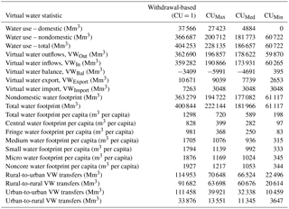
Table 3Blue virtual water transfers between urban and rural areas (Mm3).
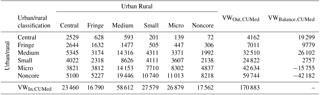
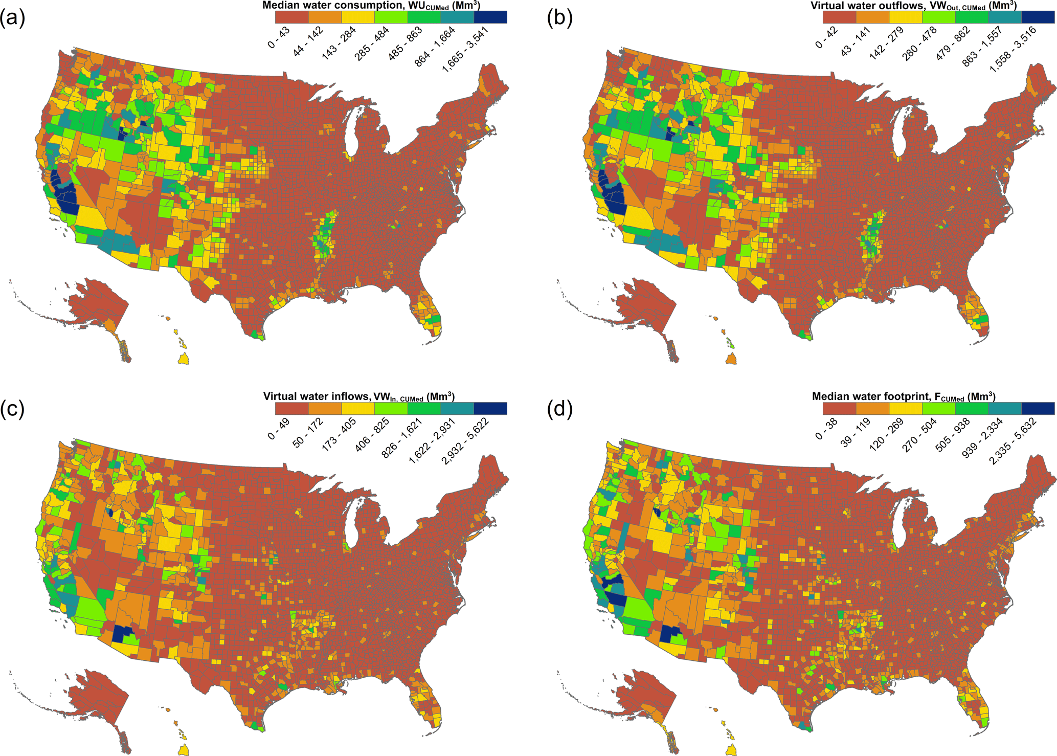
Figure 1(a) Median county-level blue water consumption in the US. (b) Blue virtual water outflows from US are concentrated in the western United States, particularly where irrigated agriculture is located, in addition to the High Plains, Mississippi Embayment, and southern Florida. (c) Blue virtual water inflows are concentrated in western US cities, western US agricultural counties, metropolitan regions in the eastern US, and in particular where a city also serves as a regional distribution center or has prominent food processing industry (Little Rock and northwestern Arkansas, Chicago, and Houston). (d) Annual withdrawal-based (CUMed) blue water footprint, FCUMed (Mm3), for US counties.
Counties in California's Central Valley – Fresno County and Tulare County located in the southern part of the Central Valley – have the largest virtual water outflows of any county in the US. Overall, the western US, the High Plains, the Mississippi Embayment, Texas Gulf Coast, and Florida provide the US with virtual water exports. Coincidentally, all these source regions are highly prone to either drought or flooding (production-level uncertainty). Large virtual water outflows are often counterbalanced by nearby virtual water inflows within the same county (Fresno County, California) or region, as is the case with Fresno County, California; Pinal County, Arizona (net outflows from irrigated agriculture); neighboring Maricopa County (net inflows to the Phoenix metropolitan area); Brazoria County, Texas (net outflows from irrigated agriculture); and Harris County (net inflows to the Houston metropolitan area) in Texas. In general, we find that the water supply chain, especially the step of the chain bringing agricultural products from the farm to handling and processing facilities where these products become “food” is mostly local and regional with a smaller but still significant transnational and international water supply chain.
3.2 Urban dependencies on rural virtual water
Circular virtual water flows – virtual water flows that originate and terminate within the same county – are highest for urban counties (Fig. 2). Conversely, rural counties often have small water footprints regardless of the presence of a large water-intensive industry, because rural populations do not consume the majority of the goods produced in those regions. If such an industry were present in a rural county, much of the water withdrawn flows out of the county as virtual water, thus counterbalancing the large withdrawals. Counties that are in the middle of the urban–rural spectrum, often a medium-to-small metropolitan area, rely heavily on agricultural products as an economic input and tend to have the largest virtual water inflows of all US counties. Medium to small cities tend to be food processing hubs where farm goods are transformed into “food” and NWED assigns irrigated agricultural blue water footprints to these hubs. We recognize that this framing of the economy emphasizes different parts of the supply chain than previous studies and we are developing methods for supply chain harmonization.
The central counties of large metropolitan areas (Central) tend to source virtual water equally across the urban–rural spectrum with a slight increase in virtual water sourcing from more medium metropolitan areas and rural counties. However, there is a comparatively small return flow of virtual water from large metropolitan areas back to counties with smaller populations (Table 3). Instead, virtual water originating from counties associated with large metropolitan areas tends to remain within that county as a circular flow or flow to other large metropolitan areas, enlarging the net VW inflow of large metropolitan areas.
Figure 2Circular blue virtual water flows (CUMed), or blue virtual water flows that originate and terminate within the same county. This is a map of the use of “local water” in the hydroeconomy. Phoenix, Arizona, is a local water hotspot.
One such county is Maricopa County, the central county of the Phoenix metropolitan area, which a “local water” hotspot where most of the water used in the community “stays local” in the form of locally consumed virtual water flowing to other users in the same community. This means the community is employing its blue water resources primarily for the hydroeconomic benefit of its local consumers and businesses. It also means that this community's dependency on its own local water resources is amplified through self-dependence, so any disruption to local water supplies in Phoenix will have a positive feedback loop on that city's economy (Rushforth and Ruddell, 2015). The Phoenix metropolitan area is notable as a major city and population center that is simultaneously a large user of irrigation water for the production of agricultural commodities, including locally consumed food products. Phoenix is also relatively isolated geographically from other metropolitan areas and therefore keeps more of its metropolitan area's virtual water within the local boundary, unlike east coast cities where intrametro trade and virtual water flows are more prevalent.
Counties that are associated with medium-sized metropolitan areas (Medium) break from large cities and their fringes and take on a different role in the system. While medium metropolitan areas are by no means small, with a population between 250 000 and 999 999, they are often colocated with large agricultural areas. For example, Ada County, Idaho (Boise metro area), Fresno County, California (Fresno metro area), or Kern County, California (Bakersfield metro) are all counties that contain medium-size metropolitan areas that are colocated with intense agricultural production. In these counties, virtual water tends to be sourced from counties that are as rural as the place of consumption or more rural. Medium-sized metropolitan areas, in particular, are the largest destination of virtual water from rural America while also being one of the largest sources of virtual water for the US, especially for large metropolitan areas – effectively linking rural and urban counties. The medium–medium urban connection is the largest link in the US virtual water flow network, and this link is dominated by the heavy industrial and bulk agricultural and processed food goods that do not tend to be produced by highly rural or densely urban areas. On a per capita basis, the Medium class of city is the core of the US hydroeconomic network. County-level virtual water flow data show that there is an urban–rural divide, suggesting that there is a fundamental difference in the roles of large urban areas, medium urban areas, and more rural communities in the US hydroeconomic network.
In the US hydroeconomy, economic sectors have different structural roles as either a virtual water sink or source depending on the degree to which a county is rural or urban. Structurally, the agricultural sector is the bulk of the rural-to-urban transfer of virtual water (59 119 Mm3), but rural-to-rural and urban-to-urban virtual water flows are also significant (53 731 and 27 743 Mm3, respectively). While similar, the livestock sector constitutes a minority of the rural-to-urban transfer of virtual water (6100 Mm3) but has little to no impact on virtual water exports. Due to the structure of the underlying commodity flow dataset, the livestock sector only includes on-site water consumption at livestock operations. Inclusion of water usage for livestock feed would, no doubt, increase virtual water transfers related to the livestock sector and a method to do so is under development for the next NWED version. The mining sector is more geographically dependent on the physical location of mineral resources and infrastructure. Therefore, while rural-to-urban virtual water flows are the largest within this sector (337 Mm3), rural-to-rural and urban-to-urban virtual water flows are also prominent (175 and 165 Mm3, respectively). In the power sector, the largest virtual water flow is from rural-to-rural (159 Mm3) followed by urban-to-urban (22 Mm3) and rural-to-urban (13 Mm3). While there are large water withdrawals associated with the power sector, water consumption is relatively low compared to other sectors. Since the results presented are for the CUMed scenario, the power sector virtual water flows are small relative to the other sectors. Finally, the industrial sector is primarily urban-to-urban virtual water transfers. Rural-to-urban virtual water transfers would only become more pronounced if Medium metropolitan areas were considered to be rural counties. While there is subjectivity to whether a county is rural or urban, especially in the middle of the urban–rural spectrum, the predominant flow of virtual water is from rural counties to urban counties.
3.3 US international virtual water imports and exports
Overall, the US is a net virtual water exporter, which qualitatively agrees with the findings from previous international virtual water flow studies (Mekonnen and Hoekstra, 2011c); the virtual water balance of the United States is −4693 Mm3. However, while our virtual water balance results agree qualitatively with previous studies, the magnitude of virtual import and export in NWED is an order of magnitude lower than previously published international virtual water trade data (Mekonnen and Hoekstra, 2011a, c). Potential reasons for this discrepancy are discussed in Sect. 3.6. Of the eight world regions in NWED, the US is a net virtual water exporter to each region, indicated by the negative virtual water balance (Table 4). The US has the largest negative virtual water balance with eastern Asia (−2081 Mm3) and Mexico (−1215 Mm3). The US is a net importer of virtual water from Central and South America (“Rest of Americas”) and Europe.
Table 4Urban–rural blue virtual water transfer by economic sector (Mm3).
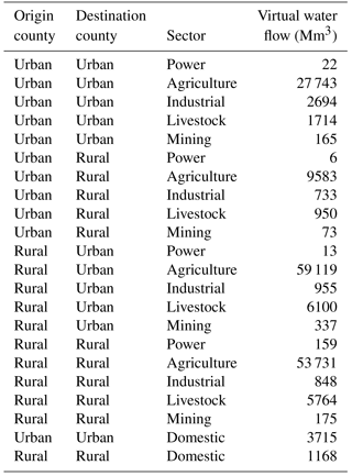
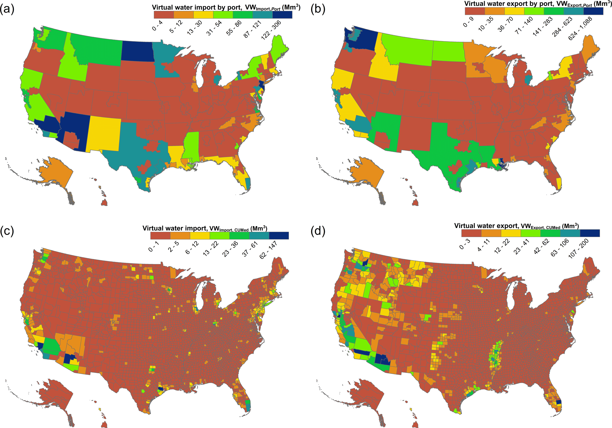
Figure 3(a) The port and border regions through which the majority of US blue virtual water imports (CUMed) enter the US market are primarily Los Angeles, New York, Arizona, North Dakota, Houston, Detroit, and Buffalo (FAZs are used for port region boundaries). (b) The ports through which the majority of US virtual water exports (CUMed) enter the global market are located in natural hazard prone areas along the west coast, Gulf Coast, and eastern seaboard. (c) Cities such as Los Angeles, Phoenix, Houston, New York City, Miami, Dallas, Seattle, and the San Francisco Bay area are the major destinations of US virtual water imports (CUMed). (d) US virtual water exports (CUMed) originate from California's Central Valley; southern California and southwestern Arizona; the Columbia River basin and the Pacific Northwest; Central Nevada and northwestern Utah; the Ogallala Aquifer region of the Midwest; the Texas Gulf Coast; the Mississippi Embayment; and southern Florida.
Virtual water export from the US is mostly agricultural commodities, such as corn, wheat, alfalfa (for which the US is a net exporter; Marston et al., 2015; Hoekstra and Wiedmann, 2014), and mining products, such as metallic and nonmetallic ores. Major virtual water exporting regions are the Central Valley of California; the deserts of California and Arizona; the High Plains, including the Ogallala Aquifer region, the Arkansas River basin, and the Platte River basin; the Columbia River basin in the Pacific Northwest; central Nevada; the Texas Gulf Coast; the Upper Missouri River basin in Montana; central and southern Florida; and the Mississippi Embayment (Fig. 3). Many of these areas are major sources of virtual water domestically within the US; however, these results show that some areas such as southwestern Idaho, Wyoming, and central Utah and New Mexico operate primarily in the domestic market, and other regions such as central Nevada (metallic ores) and western Washington (nonmetallic ores) are more prominent in the international market.
The majority of virtual water exports from the United States flow-through ports along the Gulf Coast (Houston, New Orleans, Corpus Christi, Beaumont) and the west coast (Los Angeles/Long Beach, Washington State, San Francisco, Seattle, Portland). The ports of Los Angeles and New York City receive the highest volume of virtual water imports followed by Houston and Detroit. Due to where goods for export are sourced within the US, a world region (or country) may receive a higher proportion of virtual water that originated as surface water or groundwater. For example, virtual water flows through ports in the Houston metropolitan area are dominated by groundwater sources in the Ogallala Aquifer region, the Mississippi Embayment aquifer system, and to a lesser extent the Central Valley of California, local groundwater sources, and southern Arizona (Fig. 4). Mexico, Africa, and southwestern and central Asia are the only world regions that received more virtual water that originated as groundwater (Table 5; Fig. 5), suggesting that exports to these regions are potentially more vulnerable to unsustainable, long-term groundwater management in the US than annual fluctuations in surface water availability and drought (Marston et al., 2015).
Table 5US blue virtual water exports and imports to and balances with world regions.
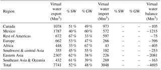
SW – Surface Water. GW – Groundwater.
While we do not address surface or ground water sustainability, vulnerability, or overdraft specifically in this paper, it is certainly desirable to combine these results with quantification of water storage and water availability, for the purpose of policy analysis. Conversely, Canada, Latin America, Europe, and Asia and Oceania have more exposure to surface water fluctuations and drought but are less exposed to unsustainable groundwater management in the US. Given that the US is a large hydrologically, agronomically, and climatically diverse country, it is not surprising that the type of water (surface water or groundwater), which an international trading partner may depend on, varies based on which part of the US is accessed, thus potentially causing two trading partners to have vastly different virtual water risk profiles.
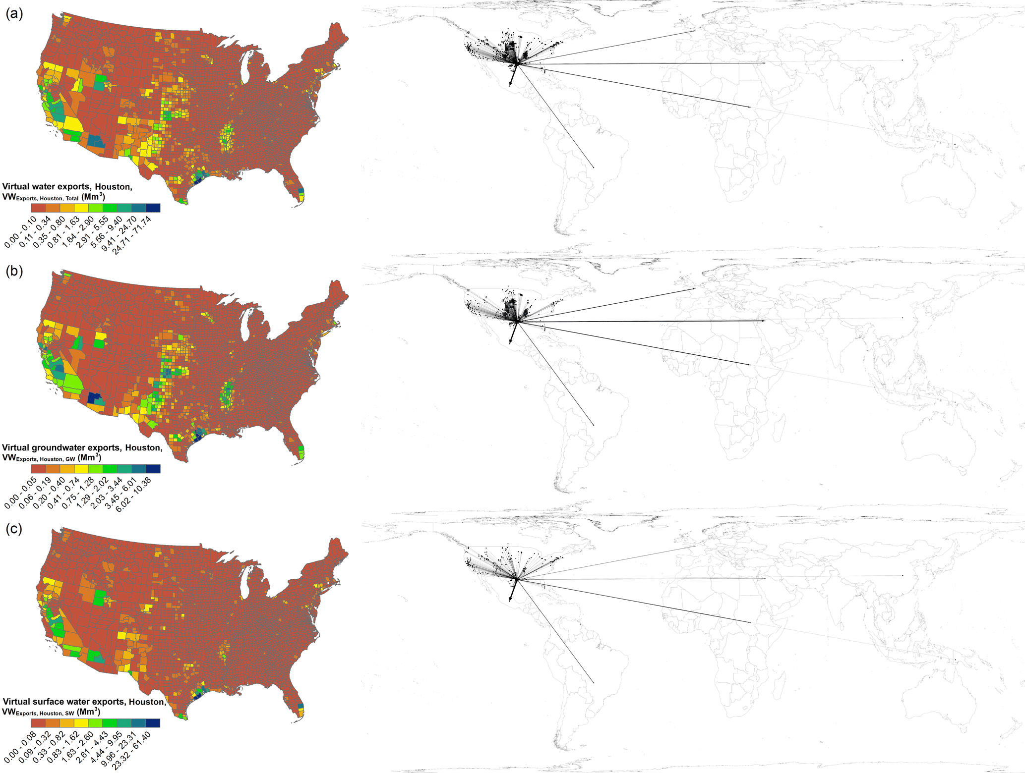
Figure 4(a) US blue virtual water exports (CUMed) through ports in the Houston metropolitan area are sourced from the Central Valley of California, central Utah and northern Utah, southern Arizona, the Ogallala Aquifer region, southern Texas and the Texas Gulf Coast, and the Mississippi Embayment aquifer region. Virtual water flows into the Houston ports and then is redistributed to the eight world regions in NWED. Mexico is the largest recipient of virtual water flows from Houston ports. (b) Virtual groundwater flow-through Houston ports is sourced from the Central Valley of California, central Utah and northern Utah, southern Arizona, the Ogallala Aquifer region, southern Texas and the Texas Gulf Coast, and the Mississippi Embayment aquifer region. (c) Virtual surface water through Houston ports is sourced from the Central Valley of California, southern California, the Phoenix metropolitan area, northern Utah, and the Texas Gulf Coast. Network maps are plotted with Gephi using the Map of Countries and GeoLayout plugins.
3.4 Structural and spatial differences in economic sector water footprints
The US water footprint is predominantly determined by the production, manufacture, and distribution of food. The agriculture (154 349 Mm3) and livestock (15 917 Mm3) economic sectors comprise 93 % of the US water footprint (181 966 Mm3), with the agriculture economic sector alone comprising 87 % of the US water footprint. Overall, the agriculture and livestock water footprint is concentrated in the western US, where there is a heavy dependence on irrigated agriculture to raise crops for human and animal consumption.
For agriculture, the Central Valley of California, the Front Range of Colorado, central and southern Arizona, and the Snake–Columbia river valley are significant geographic regions where food is grown and where irrigation is a requisite for growing crops (Fig. 6a). Where irrigated agriculture is not as prevalent, urban centers are moderate water footprints as they serve as regional distribution for food (Omaha, Nebraska; Wichita, Kansas; Dallas, Houston, and Brownsville, Texas; New Orleans, Louisiana; northwestern Arkansas; and central Florida). The US livestock footprint is more concentrated on the west coast US and Snake River Valley of Idaho; however, on the east coast, the Carolinas have the largest livestock water footprint (Fig. 6c). Outside these areas, the US livestock water footprint is concentrated around cities where there is a relatively large inflow of virtual water with little to no virtual water outflows.
Unlike the US water footprint of agriculture and livestock (Fig. 6a and 6c), in which both rural and urban counties play significant roles, the US industrial water footprint (Fig. 6b), and the US water footprint of power production and domestic water consumption (Fig. 6e and f), is dominated by urban areas. Not surprisingly, domestic and industrial water use is highly colocated with urban areas as are virtual water inflows and outflows. Major nodes in the US industrial water footprint network are Chicago, Illinois; Houston and Dallas, Texas; Los Angeles California; Seattle, Washington; Phoenix, Arizona; Las Vegas, Nevada; the Boston–Washington corridor; central and southern Florida; and each major metropolitan area east of the Mississippi River. While the same areas are important in the domestic water footprint, the US southwest – Southern California, central and southern Arizona, and Las Vegas, Nevada – have the largest domestic water footprints.
The US mining water footprint is highly dependent on the location of mineral resources in addition to processing facilities and distribution hubs. Some geographic regions with substantial mining water footprint do not have a significant water footprint in other sectors; for example, northern Alaska; west Texas; the Gulf Coast; Oklahoma; North Dakota; northern Michigan and Minnesota; and parts of Nevada, Montana, Utah, New Mexico, and Wyoming (Fig. 6d). Southern California, and to a lesser extent southern Arizona, is an exception to this because these are regions with substantial mining activity – oil and gas in Southern California and hard rock mining in Arizona – that are colocated with agricultural and industrial production in addition to high domestic water consumption.
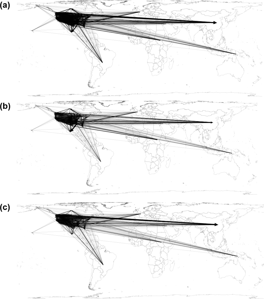
Figure 5(a) US blue virtual water exports (CUMed) through all US ports. Only flows >0.1 Mm3 are plotted in this virtual water flow network. (b) US blue virtual groundwater exports (CUMed) through all US ports. Only flows >0.1 Mm3 are plotted in this virtual water flow network. Mexico in addition to Africa and eastern Asia are a notable destination for US blue virtual groundwater exports through Gulf Coast ports. (c) US blue virtual surface water exports (CUMed) through all US ports. Only flows >0.1 Mm3 are plotted in this virtual water flow network. Eastern Asia is a notable destination for US blue virtual surface exports through west coast ports. Network maps are plotted with Gephi using the Map of Countries and GeoLayout plugins.
The net export status of a county matters because a net virtual water exporter may have a very different approach to national water policy discussions than a net importer (Fig. 7). The (usually medium-sized) communities that sit in between the net-importing and net-exporting categories may take a distinct and more balanced position on national policy. Agricultural western communities tend to be net exporters, urban communities tend to be net importers, and rural eastern communities tend to be relatively neutral; midsize urban communities, such as those commonly found in the Midwest and the east, may be relatively neutral as well.
3.5 Uncertainty introduced by consumption coefficient estimates
At the county level, blue water footprint uncertainties introduced by consumption coefficients range several orders of magnitude in cubic megameters and relative percent (Fig. 8). The small rural counties of Bristol Bay Borough, Alaska, and Kenedy County, Texas, have the smallest water footprint uncertainties (<0.50 Mm3). Los Angeles County, California, has the largest water footprint uncertainty (4050 Mm3). After Los Angeles, 3 counties have a water footprint uncertainty between 3000 and 4000 Mm3, 7 counties have a water footprint uncertainty between 2000 and 3000 Mm3, 42 counties have a water footprint uncertainty between 1000 and 2000 Mm3, and 79 counties have a water footprint uncertainty between 500 and 1000 Mm3. In relative terms, county-level water footprint uncertainty is 58.2–99.9 % of a county's total water withdrawals. Relative water footprint variation tends to increase in the eastern United States. However, in absolute terms, consumption coefficient variation is more important in the western US due to the potentially large variation in virtual water outflows from the US's largest virtual water sources.
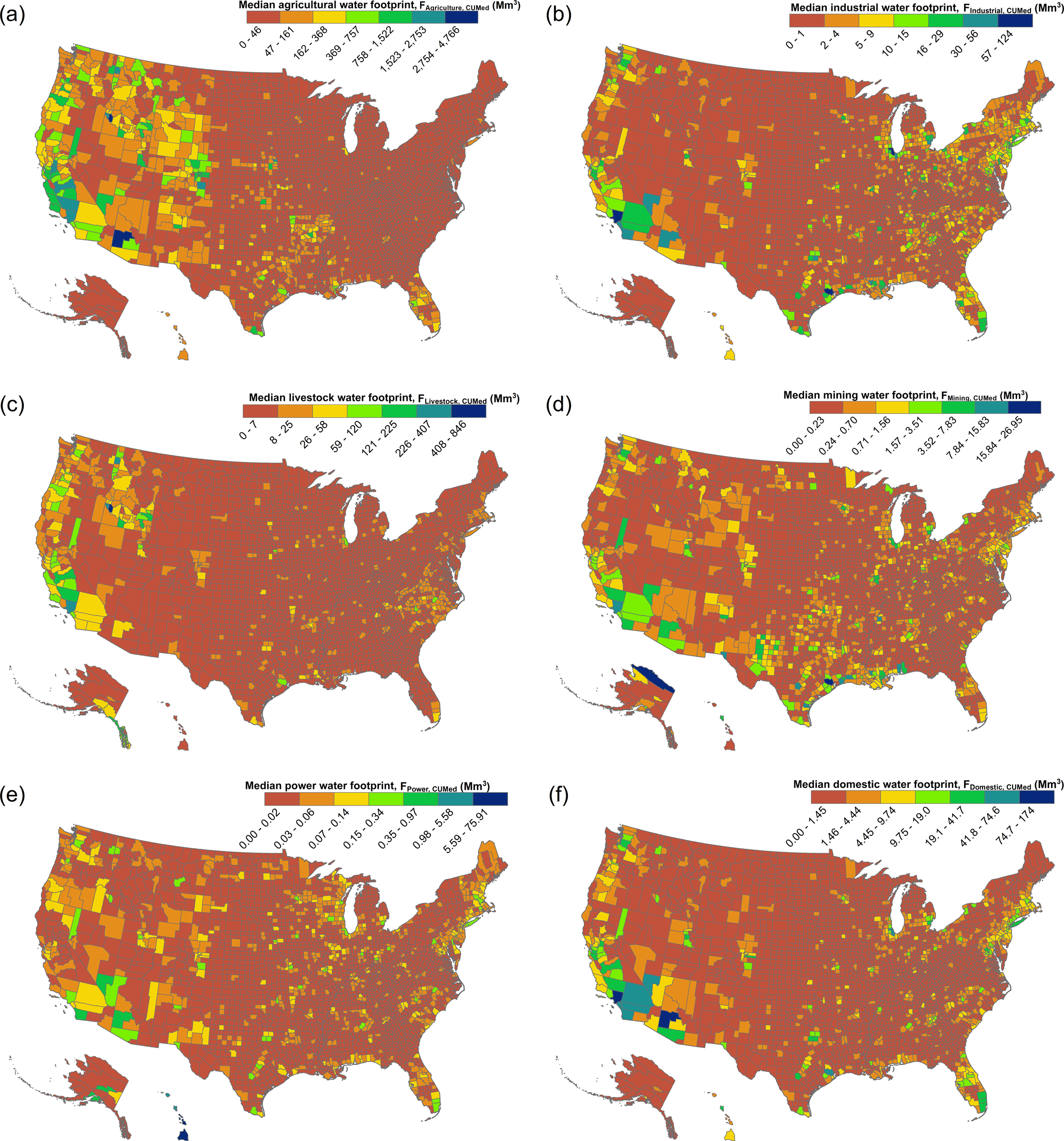
Figure 6(a) The county-level agricultural blue water footprint of the US. (b) The county-level industrial blue water footprint of the US. (c) The county-level livestock blue water footprint of the US. (d) The county-level mining blue water footprint of the US. (e) The county-level electrical power blue water footprint of the US. (f) The county-level domestic blue water footprint of the US.
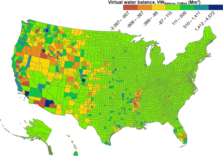
Figure 7The blue virtual water balance (VWBalance,CUMed) for each US county. Areas in the southwestern US, Central Valley of California, Snake River Valley, Mississippi Embayment, southern Florida, southern Texas, and the High Plains have virtual water outflows that outstrip virtual water inflows.
A community's role in the hydroeconomic network, and its perspective on hydroeconomic policy issues, can qualitatively change depending on our uncertainty. Due to the uncertainty introduced by consumption use coefficients, which are quite large in absolute terms, depending on consumptive use assumptions, roughly 17 % of US counties can switch between being a net virtual water importer or a net virtual water exporter as indicated by a positive or negative VWBalance (Fig. 9).
Results using the withdrawal-based (CU = 1) scenario are located in the Supplement (Table SI 4D).
3.6 Uncertainty in international virtual water flow
As mentioned in Sect. 3.4, there are several potential reasons for the discrepancy in the magnitude of virtual water flows. First, there are differences in the underlying source data for international trade and water use. NWED utilizes commodity flows modeled by FAF, which itself utilizes Census Foreign Trade Data for 2010 (Southworth et al., 2010; Hwang et al., 2016), while benchmark international virtual water trade studies utilized trade data from the International Trade Centre averaged between 1996 and 2005 (Mekonnen and Hoekstra, 2011a, c). Additionally, the source water data for the US are different. NWED utilizes USGS water withdrawal data, which are self-reported state-level data (Maupin et al., 2014; Marston et al., 2018), while benchmark international virtual water trade studies utilized CROPWAT modeling (Mekonnen and Hoekstra, 2011a, c). Secondly, despite controlling for port influences, it is likely that more virtual water is attributed to ports than necessary, which would dampen international virtual water flows in NWED. NWED has difficulty handling “flow-through” virtual waters flow that would be otherwise assigned to a point of final consumption. In this case, a flow-through entity may be assigned virtual water flow at the port or another distribution hub. Lastly, previous international virtual water studies included the water use of inputs in the virtual water flow of a commodity, e.g., the water consumption for animal feed as part of animal-product-related virtual water flow. A method to handle this is under development for the next version of NWED. While there are disadvantages to the current method in which international trade is modeled in NWED, methods to improve this aspect of the data product are ongoing and there is data structure in place to merge additional international trade flow datasets with the current NWED data structure.
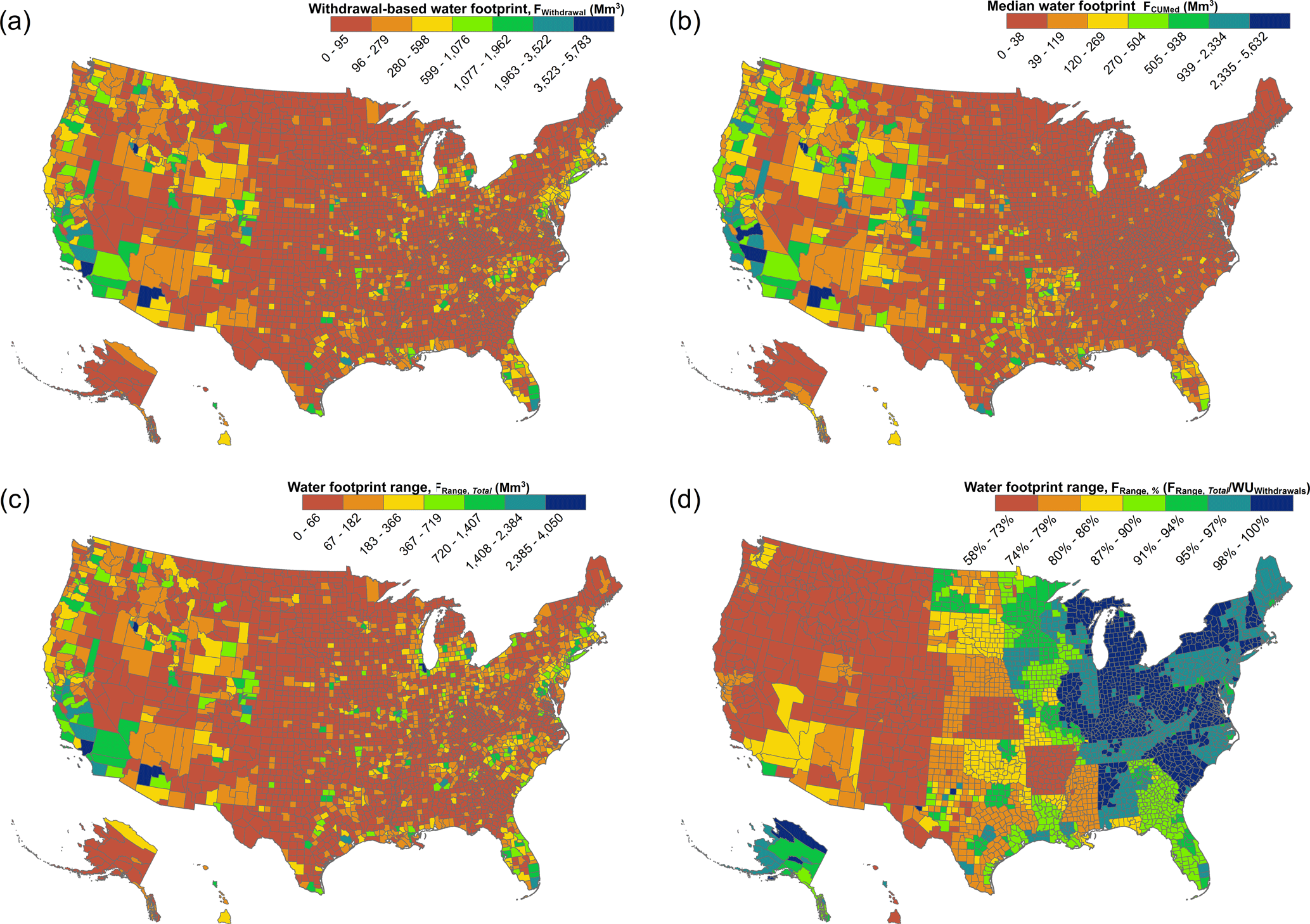
Figure 8(a) The annual withdrawal-based blue water footprint, FWithdrawal (Mm3), for US counties. (b) The annual median (CUMed) blue water footprint, FCUMed (Mm3), for US counties. The minimum scenario was constructed by applying minimum sector-level consumption coefficients. (c) The range of uncertainty in the blue water footprint, FRange (Mm3), for US counties. FRange is computed as the range between the highest and lowest water footprints of the withdrawal-based and three consumption-based scenarios. Absolute water footprint uncertainties are highest in the west, but relative uncertainties are highest in the east. (d) Relative water footprint variation tends to increase in the eastern United States and county-level water footprint uncertainty can range between 58.2 % in much of the western United States and 99.9 % in parts of the eastern United States.
3.7 Temporal uncertainty
As mentioned previously, the NWED data are limited in representativeness to roughly the 2010–2012 postrecession timeframe but are not precisely linked to a single year. Temporal uncertainty is introduced by utilizing annual timescale data. Given this, NWED data are more directly relevant to surface water management than to groundwater management because surface water has months to a few years of storage, and groundwater has centuries of storage, but in the future we could use this data to analyze sustainability and vulnerability of water usage.
Mekonnen and Hoekstra reported that the US combined blue and grey water footprint, which is the closest equivalent to the water sources used NWED, to be 320 496 Mm3 and 874 m3 per capita (Mekonnen and Hoekstra, 2011a). Results from NWED, which uses four consumptive use scenarios, for the median annual water footprint, FCUMed, of the US is 181 966 Mm3 (FWithdrawal: 400 844 Mm3; FCUMax: 222 144 Mm3; FCUMin: 61 117 Mm3 ). On a per capita basis, results from NWED found the median US water footprint ( is 589 m3 per capita (: 1298 m3 per capita; : 720 m3 per capita; : 198 m3 capita−1). Given these statistics, the reported Mekonnon and Hoekstra water footprint and per capita water footprint falls between the withdrawal-based (CU = 1) and maximum consumptive use coefficient (CUMax) scenarios. Depending on the assumptions about consumptive use at the economic-sector level, these two datasets are in rough agreement regarding the magnitude of the US water footprint.
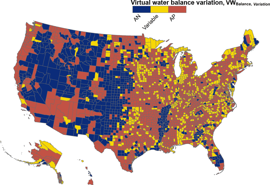
Figure 9For many counties, whether a county has a negative or positive virtual water balance varies under the consumptive use scenarios. Counties in blue always have a negative virtual water balance (AN) and virtual water outflows are always greater than virtual water inflows. Counties in red always have positive virtual water balances (AP) and virtual water inflows are always greater than virtual water outflows. Counties in yellow have borderline-neutral net virtual water balances that depend on the consumptive use uncertainty (variable).
The uncertainty introduced by water use data and consumption coefficients demonstrate the great need for the development of region-specific, sector-level water use data and consumption coefficients for the entire US. For example, water footprint uncertainty is roughly 58 to over 99 % of a county's total water footprint, which increases in the eastern United States. However, in absolute terms, consumption coefficient variation is more important in the western US due to the potentially large variation in virtual water outflows from the agricultural sector with largest blue water withdrawals. While we have presented results for the CUMed scenario in this paper, we must recognize the potentially large variation in water consumption that could exist compared to what is reported. Therefore, conclusions drawn from NWED data, as well as those drawn from the underlying water data, must recognize the large range of uncertainty with respect to water withdrawal and consumption in the US. Nevertheless, there are still general observable trends in US virtual water flows and water footprints, which are presented below.
The US hydroeconomic network is centered on cities and is dominated by the local and regional scales of trade, with medium-sized cities playing a disproportionate role. The proper framing of water governance and policy may be proportional to the structure of that network. Large cities source from all sizes of communities, but small and rural communities mostly source from other small communities, leading to a structural difference between the diversity and connectivity of urban and rural water supply chains. Further, medium-size metropolitan areas have a unique role in the US hydroeconomy as the link between rural virtual water production and urban virtual water consumption and are the most important single scale of community in the network. The US hydroeconomic network's connections and power structures are primarily local and regional except for the large metropolitan areas that operate at the national level and large-city ports that operate at the international level. This scale-specific finding is novel because most prior work on water footprints focuses on international trade.
Within the US, urban counties have a strong hydroeconomic dependence on rural counties: for the CUMed scenario there is a virtual water transfer of 114 953 Mm3 from rural counties to urban counties, roughly a third of all virtual water flow in the US, with only a 33 876 Mm3 return flow of virtual water. However, there is also strong urban-to-urban hydroeconomic dependence. The virtual water transfer between urban counties is of the same magnitude as the rural-to-urban virtual water transfers (111 458 Mm3). Taken together, rural-to-urban and urban-to-urban virtual water flow accounts for approximately 58 % of US domestic virtual water flow, illustrating the urban demand for not just water-intensive food sourced from rural counties, but also water-intensive power and industrial products sourced from urban counties. Further work on characterizing county-level virtual water flows can extend the logic developed by frameworks to characterize catchment-level water use regimes (Weiskel et al., 2007) to hydroeconomic networks. Specifically, NWED data can provide a sociohydrological extension to previous work on hydroclimatic regime classification in the US (Weiskel et al., 2014).
The networked structure of water footprint sources creates systemic exposure to surface water scarcity and groundwater unsustainability at virtual water source locations. The US and the global economy are particularly exposed to drought, and other system shocks, in the western US generally, especially in California, central and southern Arizona, Idaho, and the Great Plains. In the eastern US, exposure to drought, or other system shocks, presents in southern Texas, southern Florida, the Chicago area, and the Lower Mississippi Valley. Because the whole US, and world, depend on these water supplies, these locations should be a priority for national water policy (Cooley and Gleick, 2012; Gleick et al., 2012), for public investment in water infrastructure to manage drought (Brown and Lall, 2006; Galloway Jr., 2011), and for innovative green infrastructure and market-based solutions that address water supply and demand problems. Additionally, the ports through which virtual water flows create transportation risks posed by war, strikes, tropical storms, earthquakes, and sea level rise. These locations should be a priority for national resilience policies and efforts, and alternative freight corridors should be developed so that port closures do not impact the ability of US businesses to get their water-intensive goods to domestic and international markets (or vice versa).
Given the networked structure of the FEW system, the strong urban–rural dependence of FEW system flows, and the uncertainties presented by information gaps, future FEW system studies must address questions of worldview. For example, questions regarding which scale is the right scale (Vörösmarty et al., 2010, 2015) and which decision boundary is the best decision boundary (Rushforth et al., 2013) for understanding the FEW system interactions are dependent on the worldview of stakeholders and policymakers. In the US, the direct and indirect transfer of FEW system resources is concentrated at the mesoscale – regions and/or county equivalents – and not the national or global scales. This has implications for developing robust FEW system policy: the mesoscale is a manageable scale and there is the ability to manage aspects of FEW systems and craft FEW system interventions at this scale through extant and novel local and regional governance systems. For example, downstream-driven, market-based supply chain governance of “soft” supply chains by major retailers and distributors; downstream-driven city-driven governance via their hard infrastructures (McManamay et al., 2017); upstream-driven, watershed- or river-driven governance wherein infrastructure managers consider how the services of their water propagate through the economy; or FEW governance where food, energy, and water agents work together because these sectors have the largest footprints.
NWED provides insight into which sectors and geographic areas need to be prioritized in the development of these consumption coefficients. The lack of certainty with regard to consumption coefficients (Sect. 3.5) limits the ability to estimate or gauge one area's exposure to hydrological hazards in another area in its supply chain and must be addressed through the development of county- or region-specific and economic-sector-specific consumption coefficients. We suggest starting with cities and irrigated agriculture in the western US due to the major influence that consumption coefficients have on water footprints, and because we lack locally accurate consumption coefficients to distinguish between regions this prevents us from accurately assessing local water balances or scarcity.
Despite basic limitations imposed by the primary data sources, NWED is a robustly quantified blue water footprint; future refinements to NWED will seek to address these limitations and add additional functionality, such as increased resolution on pass-through commodity flows. The empirical basis of this analysis, along with its economic completeness and spatial detail, make this result a landmark resource in the scientific discussion of water footprints, virtual water flow, and the sustainability and resilience of a nation's water resources in the connected global economy.
Please contact Richard R. Rushforth for NWED v 1.1 code availability.
NWED version 1.1 is available at the Hydroshare data repository and can be accessed at https://www.hydroshare.org/resource/84d1b8b60f274ba4be1558 81129561a9/ (Rushforth and Ruddell, 2018).
Data from NWED 1.0 have previously been published in Rushforth and Ruddell (2016). While the methodology is largely the same, there are key differences between the two versions of NWED:
-
If updated disaggregation and attraction factors were available, these factors were updated.
-
Specifically, agricultural disaggregation factors were updated at the crop level using the latest USDA NASS.
-
Additionally, the mining sector been updated to have commodity-code-specific disaggregation factors using the location of mines and mineral production as disaggregation factors rather than employment.
-
The power sector and domestic sector has been added to NWED version 1.1.
-
Export virtual water flows have been disaggregated from virtual water flows to port cities.
-
Import virtual water flows have been added to NWED version 1.1.
-
The CUMax, CUMed, and CUMin consumption scenarios were added to NWED version 1.1.
-
Groundwater and surface water disaggregation of virtual water flows for withdrawal, CUMax, CUMed, and CUMin scenarios were added.
-
Agricultural sector: NWED sector comprised of farm-based activities to grow crops for food or industrial purposes. Irrigation is the primary water use activity in the agricultural sector (Maupin et al., 2014).
-
Attraction factor: A fraction used to disaggregate commodity flows on the consumption side. In NWED 1.1, population is used as an attraction factor. Each county within a FAZ is assigned a fraction equivalent to its percent of the total population.
-
County: A county or county equivalent (parish, borough, Washington DC, or a independent city) is a substate geographic scale that is roughly equivalent to the mesoscale.
-
Destination: The geographic location where a commodity flow terminates.
-
Freight analysis zone (FAZ): A group of counties that represents a metropolitan statistical area, census statistical area, or remainder of a state (Southworth et al., 2010; Hwang et al., 2016)
-
Industrial sector: Economic sector that produces industrial goods. Water use in the industrial sector includes “fabricating, processing, washing, diluting, cooling, or transporting a product; incorporating water into a product; or for sanitation needs within the manufacturing facility” (Maupin et al., 2014).
-
Large central metro counties: US counties with more than 1 million inhabitants that are the central county of a metropolitan statistical area (Ingram and Franco, 2012).
-
Large fringe counties: US counties with more than 1 million inhabitants that are not the central county of a metropolitan statistical area (Ingram and Franco, 2012).
-
Livestock sector: Economic sector comprised of the raising of animals for animal products in addition to aquaculture activities. Water use in the livestock sector only includes direct water use at livestock, and related facilities (Maupin et al., 2014).
-
Medium metro counties: US counties with between 250 000 and 999 999 inhabitants (Ingram and Franco, 2012).
-
Micropolitan counties: US counties with between 10 000 and 49 999 inhabitants that have an urban cluster (Ingram and Franco, 2012).
-
Mining sector: Economic sector comprised of mineral producing activities, including metallic and nonmetallic ore, in addition to sand and gravel, crude petroleum, and natural gas. Water use activities in the mining sector include “the extraction of minerals that may be in the form of solids, such as coal, iron, sand, and gravel; liquids, such as crude petroleum; and gases, such as natural gas” (Maupin et al., 2014).
-
Noncore counties: US counties with between 10 000 and 49 999 inhabitants that do not have an urban cluster (Ingram and Franco, 2012).
-
Origin: The geographic location where a commodity flow originates.
-
Production factor: A fraction used to disaggregate commodity flows on the production side. In NWED 1.1, multiple production factors are used that are specific to the economic sector. Each county within a FAZ is assigned a fraction equivalent to its percentage of the total population.
-
Power sector: NWED sector comprised of electric generating stations, which includes thermoelectric and nonthermoelectric facilities (renewable energy sources). Water is used at thermoelectric generation stations in addition to hydroelectric facilities.
-
Small metro counties: US counties with metropolitan statistical areas with less than 250 000 inhabitants (Ingram and Franco, 2012).
-
Virtual water: Also known as indirect water or embodied water, virtual water has been studied as a strategic resource for two decades as it allows geographic areas (country, state, province, city) to access more water than is physically available (Allan, 1998, 2003; Suweis et al., 2011; Dalin et al., 2012; Dang et al., 2015; Zhao et al., 2015; Marston et al., 2015).
-
Virtual water inflows into a geographic area (VWIn): The volume of water indirectly consumed to produce goods or services produced outside a geographic boundary of interest for consumption within that geographic boundary of interest.
-
Virtual water outflows from a geographic area (VWOut): The volume of water used to produce goods or services that are consumed outside of geographic boundary of interest.
-
Virtual water balance of a geographic area (VWNet): Virtual water inflows minus virtual water outflows for a geographic boundary of interest.
-
Water footprint: The volume of surface water and groundwater consumed during the production of a good or service and is also called the virtual water content of a good or service (Mekonnen and Hoekstra, 2011b).
-
Water footprint of consumption: Water consumption for local use in addition to virtual water import (Mekonnen and Hoekstra, 2011a)
-
Water footprint of a geographic area (F): The volume of water representing direct water consumption plus virtual water inflows minus virtual water outflows for a geographic boundary of interest. A per capita water footprint (F′) is F divided by the population within the geographic boundary of interest.
-
Water footprint of production: The total volume of water consumed with a geographic boundary, including water consumption for local use less virtual water export (Mekonnen and Hoekstra, 2011a).
-
Water consumption (C): The total volume of water consumed from a water source, when consumption is withdrawals minus return flows. A water source is either surface water or groundwater. NWED utilizes four consumptive use scenarios based on a withdrawal-based scenario, and minimum, median, and maximum consumptive use scenario. Consumptive use scenarios are based on reports published by the United States Geological Survey (Shaffer and Runkle, 2007).
-
Water withdrawal (W): The total volume of water withdrawn from a water source. A water source is either surface water or groundwater.
Each commodity trade linkage is measured by 15 metrics:
The supplement related to this article is available online at: https://doi.org/10.5194/hess-22-3007-2018-supplement.
RRR developed the NWED methodology and the executed code to carry out the methodology. RRR wrote the paper with help from BLR.
The authors declare that they have no conflict of interest.
The opinions expressed by authors contributing to this journal do not necessarily reflect the opinions of the Hydrology and Earth System Sciences Journal or the institutions with which the authors are affiliated. The opinions expressed are those of the authors, and not necessarily the National Science Foundation.
Funding for this research was provided by the National Science Foundation
under award number ACI-1639529 (FEWSION). The
authors would like to acknowledge input from colleagues on the development
of this paper and the anonymous peer referees of this paper. Finally,
the authors would like to thank the anonymous referees of this paper for
their thorough and constructive comments.
Edited by: Uwe Ehret
Reviewed by: two anonymous referees
Allan, J. A.: Virtual Water: A Strategic Resource Global Solutions to Regional Deficits, Ground Water, 36, 545–546, https://doi.org/10.1111/j.1745-6584.1998.tb02825.x, 1998.
Allan, J. A.: Virtual water-the water, food, and trade nexus. Useful concept or misleading metaphor?, Water int., 28, 106–113, 2003.
Archfield, S., Vogel, R., Steeves, P., Brandt, S., Weiskel, P., and Garabedian, S.: The Massachusetts Sustainable-Yield Estimator: A decision-support tool to assess water availability at ungaged sites in Massachusetts, US Geological Survey Scientific Investigations Report 2009–5227, 1-41, 2010.
Bialek, J.: Identification of source-sink connections in transmission networks, in Fourth International Conference on Power System Control and Management (Conf. Publ. No. 421), 200–204., https://doi.org/10.1049/cp:19960264, 1996.
Bialek, J.: Tracing the flow of electricity, IEE Proceedings-Generation, Transmission and Distribution, 143, 313–320, 1996b.
Bialek, J. and Kattuman, P.: Proportional sharing assumption in tracing methodology, IEE Proceedings-Generation, Transmission and Distribution, 151, 526–532, 2004.
Brown, C. and Lall, U.: Water and economic development: The role of variability and a framework for resilience, Nat. Resour. Forum, 30, 306–317, https://doi.org/10.1111/j.1477-8947.2006.00118.x, 2006.
Bujanda, A., Villa, J., and Williams, J.: Development of Statewide Freight Flows Assignment Using the Freight Analysis Framework (Faf 3), Journal of Behavioural Economics, Finance, Entrepreneurship, Accounting and Transport, 2, 47–57, 2014.
Bureau of Labor Statistics: Quarterly Census of Employment and Wages, available at: https://www.bls.gov/cew/ (last access: 8 September 2017), 2012.
Castle, S. L., Thomas, B. F., Reager, J. T., Rodell, M., Swenson, S. C., and Famiglietti, J. S.: Groundwater depletion during drought threatens future water security of the Colorado River Basin, Geophys. Res. Lett., 41, 5904–5911, 2014.
Christian-Smith, J., Levy, M. C., and Gleick, P. H.: Maladaptation to drought: a case report from California, USA, Sustain. Sci., 10, 491–501, https://doi.org/10.1007/s11625-014-0269-1, 2015.
Cohen, S. M., Averyt, K., Macknick, J., and Meldrum, J.: Modeling Climate-Water Impacts on Electricity Sector Capacity Expansion, 46094, V002T10A007, https://doi.org/10.1115/POWER2014-32188, 2014.
Cooley, H. and Gleick, P. H.: U.S. Water Policy Reform, in: The World's Water Volume 7: The Biennial Report on Freshwater Resources, Island Press, 1–424, 2012.
Dalin, C., Konar, M., Hanasaki, N., Rinaldo, A., and Rodriguez-Iturbe, I.: Evolution of the global virtual water trade network, P. Natl. Acad. Sci. USA, 109, 5989–5994, 2012.
Dang, Q., Lin, X., and Konar, M.: Agricultural virtual water flows within the United States, Water Resour. Res., 51, 973–986, https://doi.org/10.1002/2014WR015919, 2015.
De Jong, G., Gunn, H., and Walker, W.: National and international freight transport models: an overview and ideas for future development, Transport Rev., 24, 103–124, 2004.
Diffenbaugh, N. S., Swain, D. L., and Touma, D.: Anthropogenic warming has increased drought risk in California, P. Natl. Acad. Sci. USA, 112, 3931–3936, 2015.
Energy Information Administration: Form EIA-923, available at: https://www.eia.gov/electricity/data/eia923/ (last access: 20 September 2018), 2017.
Eurek, K., Cole, W., Bielen, D., Blair, N., Cohen, S., Frew, B., Ho, J., Krishnan, V., Mai, T., and Sigrin, B.: Regional Energy Deployment System (ReEDS) Model Documentation: Version 2016, NREL (National Renewable Energy Laboratory (NREL), Technical Report NREL/TP-6A20-67067, Golden, CO, USA, 1–101, 2016.
Famiglietti, J. S. and Rodell, M.: Water in the balance, Science, 340, 1300–1301, 2013.
Galloway Jr., G.: A plea for a coordinated national water policy, Bridge, 41, 37–46, 2011.
Gleick, P. H.: Global Freshwater Resources: Soft-Path Solutions for the 21st Century, Science, 302, 1524–1528, https://doi.org/10.1126/science.1089967, 2003.
Gleick, P. H., Christian-Smith, J., and Cooley, H.: A Twenty-First Century U.S. Water Policy, OUP, New York, NY, USA, 1–304, 2012.
Harris, G. A., Anderson, M. D., Farrington, P. A., Schoening, N. C., Swain, J. J., and Sharma, N. S.: Developing Freight Analysis Zones at a State Level: A Cluster Analysis Approach, J. Transp. Res. Forum, 49, 59–68, https://doi.org/10.5399/osu/jtrf.49.1.2521, 2010.
Hoekstra, A. Y. and Wiedmann, T. O.: Humanity's unsustainable environmental footprint, Science, 344, 1114–1117, https://doi.org/10.1126/science.1248365, 2014.
Hoekstra, A. Y., Chapagain, A. K., Aldaya, M. M., and Mekonnen, M. M.: The water footprint assessment manual: Setting the global standard, Earthscan, London, UK, 53–60, 2012
Hwang, H.-L., Hargrove, S., Chin, S.-M., Wilson, D., Lim, H., Chen, J., Taylor, R., Peterson, B., and Davidson, D.: Building the FAF4 Regional Database: Data Sources and Estimation Methodologies, Laboratory, O. R. N., Oak Ridge, TN, USA, 1–77, 2016.
Ingram, D. D. and Franco, S. J.: NCHS urban-rural classification scheme for counties, Vital and health statistics. Series 2, 154, Data evaluation and methods research, 1–65, 2012.
Joseph, M. A., Charles, J. V., Robert, J. N., Dennis, P. L., and Claudia, P.-W.: A grand challenge for freshwater research: understanding the global water system, Environ. Res. Lett., 3, 010202, https://doi.org/10.1088/1748-9326/3/1/010202, 2008.
Kennedy, C. A., Stewart, I., Facchini, A., Cersosimo, I., Mele, R., Chen, B., Uda, M., Kansal, A., Chiu, A., Kim, K.-g., Dubeux, C., Lebre La Rovere, E., Cunha, B., Pincetl, S., Keirstead, J., Barles, S., Pusaka, S., Gunawan, J., Adegbile, M., Nazariha, M., Hoque, S., Marcotullio, P. J., González Otharán, F., Genena, T., Ibrahim, N., Farooqui, R., Cervantes, G., and Sahin, A. D.: Energy and material flows of megacities, P. Natl. Acad. Sci. USA, 112, 5985–5990, https://doi.org/10.1073/pnas.1504315112, 2015.
Liu , J., Dietz, T., Carpenter, S. R., Alberti, M., Folke, C., Moran, E., Pell, A. N., Deadman, P., Kratz, T., Lubchenco, J., Ostrom, E., Ouyang, Z., Provencher, W., Redman, C. L., Schneider, S. H., and Taylor, W. W.: Complexity of Coupled Human and Natural Systems, Science, 317, 1513–1516, https://doi.org/10.1126/science.1144004, 2007.
Macknick, J., Newmark, R., Heath, G., and Hallett, K.: Operational water consumption and withdrawal factors for electricity generating technologies: a review of existing literature, Environ. Res. Lett., 7, 045802, https://doi.org/10.1088/1748-9326/7/4/045802, 2012.
Macknick, J., Cohen, S., Newmark, R., Martinez, A., Sullivan, P., and Tidwell, V.: Water constraints in an electric sector capacity expansion model, National Renewable Energy Laboratory (NREL), Golden, CO, United States, 1–21, 2015.
Mann, M. E. and Gleick, P. H.: Climate change and California drought in the 21st century, P. Natl. Acad. Sci. USA, 112, 3858–3859, 2015.
Marston, L., Konar, M., Cai, X., and Troy, T. J.: Virtual groundwater transfers from overexploited aquifers in the United States, P. Natl. Acad. Sci. USA, 112, 8561–8566, https://doi.org/10.1073/pnas.1500457112, 2015.
Marston, L., Ao, Y., Konar, M., Mekonnen, M. M., and Hoekstra, A. Y.: High-Resolution Water Footprints of Production of the United States, Water Resour. Res., 54, 2288–2316, https://doi.org/10.1002/2017WR021923, 2018.
Maupin, M. A., Kenny, J. F., Hutson, S. S., Lovelace, J. K., Barber, N. L., and Linsey, K. S.: Estimated use of water in the United States in 2010: U.S. Geological Survey Circular 1405, 56 pp., https://doi.org/10.3133/cir1405, 2014.
Mayer, A., Mubako, S., and Ruddell, B. L.: Developing the greatest Blue Economy: Water productivity, fresh water depletion, and virtual water trade in the Great Lakes basin, Earths Future, 4, 282–297, 2016.
McManamay, R. A., Surendran Nair, S., DeRolph, C. R., Ruddell, B. L., Morton, A. M., Stewart, R. N., Troia, M. J., Tran, L., Kim, H., and Bhaduri, B. L.: US cities can manage national hydrology and biodiversity using local infrastructure policy, Proc. Natl. Acad. Sci., 114, 9581–9586, https://doi.org/10.1073/pnas.1706201114, 2017.
McNutt, M.: The drought you can't see, Science, 345, 1543 pp., https://doi.org/10.1126/science.1260795, 2014.
Mekonnen, M. M. and Hoekstra, A. Y.: National water footprint accounts: the green, blue and grey water footprint of production and consumption, Value of Water Research Report Series No. 50, UNESCO-IHE, Delft, the Netherlands, 1–44, 2011a.
Mekonnen, M. M. and Hoekstra, A. Y.: The green, blue and grey water footprint of crops and derived crop products, Hydrol. Earth Syst. Sci., 15, 1577–1600, https://doi.org/10.5194/hess-15-1577-2011, 2011b.
Mekonnen, M. M. and Hoekstra, A. Y.: National water footprint accounts: the green, blue and grey water footprint of production and consumption, Value of Water Research Report Series No. 50, UNESCO-IHE, 2, Appendix I-1 to Appendix XI-3, Delft, the Netherlands, 2011c.
Mubako, S. T., Ruddell, B. L., and Mayer, A. S.: Relationship between water withdrawals and freshwater ecosystem water scarcity quantified at multiple scales for a Great Lakes watershed, J. Water Res. Pl., 139, 671–681, 2013.
Ruddell, B. L., Adams, E. A., Rushforth, R., and Tidwell, V. C.: Embedded resource accounting for coupled natural-human systems: An application to water resource impacts of the western U.S. electrical energy trade, Water Resour. Res., 50, 7957–7972, https://doi.org/10.1002/2013WR014531, 2014.
Rushforth, R. and Ruddell, B.: The Hydro-Economic Interdependency of Cities: Virtual Water Connections of the Phoenix, Arizona Metropolitan Area, Sustainability, 7, 8522, https://doi.org/10.3390/su7078522, 2015.
Rushforth, R. R. and Ruddell, B. L.: The vulnerability and resilience of a city's water footprint: The case of Flagstaff, Arizona, USA, Water Resources Research, 52, 2698–2714, 2016.
Rushforth, R. R. and Ruddell, B. L.: National Water Economy Database, version 1.1, HydroShare, https://doi.org/10.4211/hs.84d1b8b60f274ba4be155881129561a9, 2018
Rushforth, R. R., Adams, E. A., and Ruddell, B. L.: Generalizing ecological, water and carbon footprint methods and their worldview assumptions using Embedded Resource Accounting, Water Resources and Industry, 1, 77–90, 2013.
Seager, R., Ting, M., Held, I., Kushnir, Y., Lu, J., Vecchi, G., Huang, H.-P., Harnik, N., Leetmaa, A., Lau, N.-C., Li, C., Velez, J., and Naik, N.: Model Projections of an Imminent Transition to a More Arid Climate in Southwestern North America, Science, 316, 1181–1184, https://doi.org/10.1126/science.1139601, 2007.
Seager, R., Goddard, L., Nakamura, J., Henderson, N., and Lee, D. E.: Dynamical Causes of the 2010/11 Texas–Northern Mexico Drought, J. Hydrometeorol., 15, 39–68, https://doi.org/10.1175/jhm-d-13-024.1, 2014.
Seager, R., Hoerling, M., Schubert, S., Wang, H., Lyon, B., Kumar, A., Nakamura, J., and Henderson, N.: Causes of the 2011–14 California Drought, J. Climate, 28, 6997–7024, https://doi.org/10.1175/jcli-d-14-00860.1, 2015.
Shaffer, K. and Runkle, D. L.: Consumptive Water, Use Coefficients for the Great Lakes Basin and Climatically Similar Areas, US Geological Survey Reston, VA, 1–191, 2007.
Southworth, F., Davidson, D., Hwang, H., Peterson, B. E., and Chin, S.: The freight analysis framework, version 3: Overview of the FAF3 National Freight Flow Tables, Prepared for Federal highway administration Office of freight management and operations, Federal highway administration US Department of Transportation, Washington, DC, 2010.
Suweis, S., Konar, M., Dalin, C., Hanasaki, N., Rinaldo, A., and Rodriguez-Iturbe, I.: Structure and controls of the global virtual water trade network, Geopys. Res. Lett., 38, L10403, https://doi.org/10.1029/2011GL046837, 2011.
U.S. Geological Service: Active Mines and Mineral Processing Plants in the United States in 2003, 2005.
U.S. Census Bureau, Bureau of Transportation Statistics: 2012 Commodity Flow Survey Standard Classification of Transported Goods (SCTG): SCTG COMMODITY CODES (CFS-1200) Washington D.C., available at: https://www.census.gov/econ/cfs/2012/2012_manual.pdf (last access: 8 September 2017), 2011.
U.S. Census Bureau: Annual Estimates of the Resident Population: April 1, 2010 to July 1, 2013, Washington, DC, available at: https://factfinder.census.gov/faces/tableservices/jsf/pages/productview.xhtml?src=bkmk (last access: 2 May 2018), 2014.
U.S. Census Bureau: Commodity Flow Survey – About the Survey, available at: https://www.census.gov/econ/cfs/about_the_survey.html (last access: 8 September 2017), 2016.
USDA National Agricultural Statistics Service: Census of Agriculture, 1, Washington, DC, available at: ftp://ftp.nass.usda.gov/quickstats/qs.census2012.txt.gz (last access: 28 March 2017), 2012.
Viswanathan, K., Beagan, D., Mysore, V., and Srinivasan, N.: Disaggregating Freight Analysis Framework Version 2 Data for Florida: Methodology and Results, Transportation Research Record: Journal of the Transportation Research Board, 2049, 167–175, https://doi.org/10.3141/2049-20, 2008.
Vörösmarty, C. J., Green, P., Salisbury, J., and Lammers, R. B.: Global water resources: vulnerability from climate change and population growth, Science, 289, 284–288, 2000.
Vörösmarty, C. J., McIntyre, P. B., Gessner, M. O., Dudgeon, D., Prusevich, A., Green, P., Glidden, S., Bunn, S. E., Sullivan, C. A., Liermann, C. R., and Davies, P. M.: Global threats to human water security and river biodiversity, Nature, 467, https://doi.org/10.1038/nature09440, 555–561, 2010.
Vörösmarty, C. J., Hoekstra, A. Y., Bunn, S. E., Conway, D., and Gupta, J.: Fresh water goes global, Science, 349, 478–479, https://doi.org/10.1126/science.aac6009, 2015.
Weiskel, P. K., Vogel, R. M., Steeves, P. A., Zarriello, P. J., DeSimone, L. A., and Ries, K. G.: Water use regimes: Characterizing direct human interaction with hydrologic systems, Water Resour. Res., 43, W04402, https://doi.org/10.1029/2006WR005062, 2007.
Weiskel, P. K., Brandt, S. L., DeSimone, L. A., Ostiguy, L. J., and Archfield, S. A.: Indicators of streamflow alteration, habitat fragmentation, impervious cover, and water quality for Massachusetts stream basins, US Department of the Interior, US Geological Survey, Reston, Virginia, 1–67, 2010.
Weiskel, P. K., Wolock, D. M., Zarriello, P. J., Vogel, R. M., Levin, S. B., and Lent, R. M.: Hydroclimatic regimes: a distributed water-balance framework for hydrologic assessment, classification, and management, Hydrol. Earth Syst. Sci., 18, 3855–3872, https://doi.org/10.5194/hess-18-3855-2014, 2014.
World Bank: Water productivity, total (constant 2010 US$ GDP per cubic meter of total freshwater withdrawal): https://data.worldbank.org/indicator/ER.GDP.FWTL.M3.KD, last access: 10 September 2017.
Zetland, D.: The End of Abundance: Economic Solutions to Water Scarcity, Aguanomics Press, California, USA, 1–294, 2011.
Zhao, X., Liu, J., Liu, Q., Tillotson, M. R., Guan, D., and Hubacek, K.: Physical and virtual water transfers for regional water stress alleviation in China, P. Natl. Acad. Sci. USA, 112, 1031–1035, https://doi.org/10.1073/pnas.1404130112, 2015.
- Abstract
- Introduction
- Methods
- Results
- Conclusions
- Code availability
- Data availability
- Appendix A: Difference between NWED version 1.0 and 1.1
- Appendix B: NWED glossary
- Appendix C: Commodity trade linkage metrics
- Author contributions
- Competing interests
- Disclaimer
- Acknowledgements
- References
- Supplement