Using hydraulic head, chloride and electrical conductivity data to distinguish between mountain-front and mountain-block recharge to basin aquifers

Numerous basin aquifers in arid and semi-arid regions of the world derive a significant portion of their recharge from adjacent mountains. Such recharge can effectively occur through either stream infiltration in the mountain-front zone (mountain-front recharge, MFR) or subsurface flow from the mountain (mountain-block recharge, MBR). While a thorough understanding of recharge mechanisms is critical for conceptualizing and managing groundwater systems, distinguishing between MFR and MBR is difficult. We present an approach that uses hydraulic head, chloride and electrical conductivity (EC) data to distinguish between MFR and MBR. These variables are inexpensive to measure, and may be readily available from hydrogeological databases in many cases. Hydraulic heads can provide information on groundwater flow directions and stream–aquifer interactions, while chloride concentrations and EC values can be used to distinguish between different water sources if these have a distinct signature. Such information can provide evidence for the occurrence or absence of MFR and MBR. This approach is tested through application to the Adelaide Plains basin, South Australia. The recharge mechanisms of this basin have long been debated, in part due to difficulties in understanding the hydraulic role of faults. Both hydraulic head and chloride (equivalently, EC) data consistently suggest that streams are gaining in the adjacent Mount Lofty Ranges and losing when entering the basin. Moreover, the data indicate that not only the Quaternary aquifers but also the deeper Tertiary aquifers are recharged through MFR and not MBR. It is expected that this finding will have a significant impact on the management of water resources in the region. This study demonstrates the relevance of using hydraulic head, chloride and EC data to distinguish between MFR and MBR.

1 Introduction

Numerous basin aquifers in arid and semi-arid regions receive a significant portion of their recharge from adjacent mountains, largely because the latter typically benefit from higher precipitation and lower evapotranspiration (Winograd et al., 1998; Wilson and Guan, 2004; Earman et al., 2006). Two recharge mechanisms can be recognized (Wahi et al., 2008): mountain-front recharge (MFR), which predominantly consists of stream infiltration in the mountain-front zone, and mountain-block recharge (MBR), which consists of subsurface flow from the mountain towards the basin. Here the mountain-front zone is defined after Wilson and Guan (2004) as the upper zone of the basin, between the basin floor and the mountain block (Fig. 1a). The term MFR has traditionally been used to encompass the two recharge mechanisms described above, but it may be more appropriate to use it for the first one only. Following Wahi et al. (2008), the collective process of MFR and MBR is referred to as mountain system recharge (MSR).

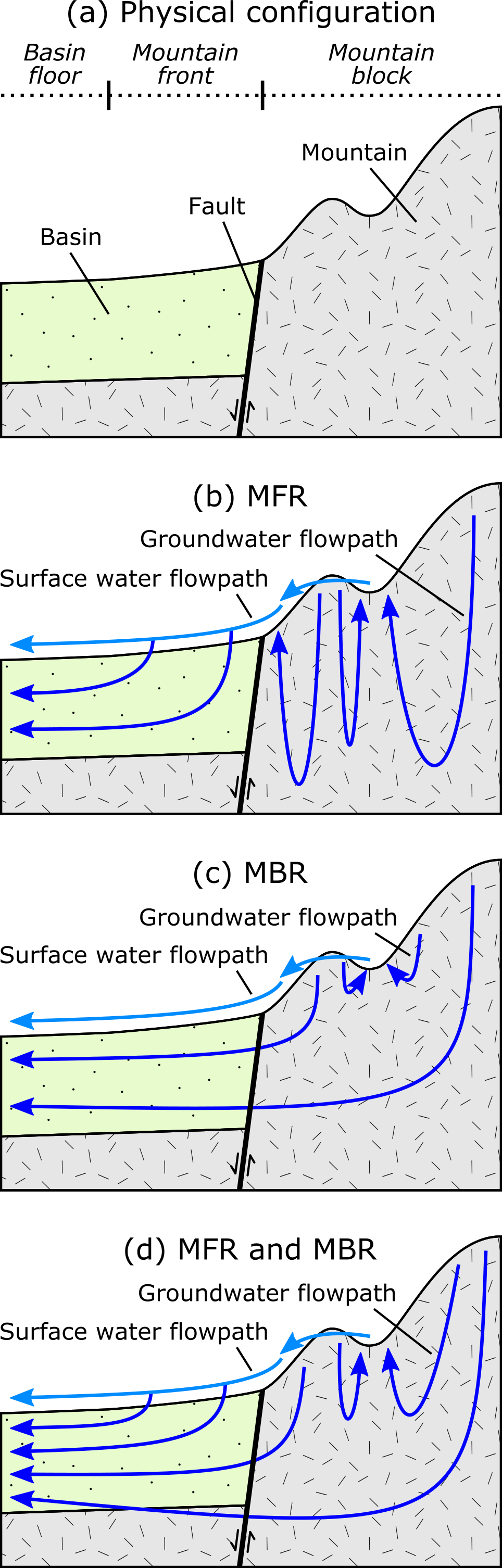
Figure 1 Conceptual models of the transition between mountain and basin: (a) physical configuration and (b–c) possible conceptualizations of MSR where (b) MFR dominates, (c) MBR dominates, and (d) both MFR and MBR are significant.

The distinction between MFR and MBR is important. The conceptualization of a basin groundwater system critically depends on whether recharge occurs through MFR or MBR, as each of these mechanisms implies different groundwater flow paths, groundwater age and geochemical characteristics. MFR and MBR can also imply different responses to land and water resource management practices (both in the basin and the mountain) as well as to climate change. A good understanding of these mechanisms is thus essential for an effective coordinated management approach of water resources in basins and adjacent mountains (Manning and Solomon, 2003; Wilson and Guan, 2004).

While various methods exist to estimate MSR as a bulk, characterizing the individual contributions of MFR and MBR is difficult. For instance, Darcy's law calculations and inverse groundwater flow modelling typically provide bulk MSR estimates (e.g. Hely et al., 1971; Anderson, 1972; Maurer and Berger, 1997; Siade et al., 2015). It is possible to consider MFR and MBR independently in a groundwater flow model, but the solution to the inverse problem is more likely to be non-unique (e.g. Bresciani et al., 2015b). The water balance and chloride mass balance methods also provide bulk MSR estimates when the analysis is performed at the base of the mountain-front zone or further downstream in the basin (e.g. Maxey and Eakin, 1949; Dettinger, 1989). Environmental tracers such as noble gases (e.g. Manning and Solomon, 2003), stable isotopes (e.g. Liu and Yamanaka, 2012) and radioactive isotopes (e.g. Plummer et al., 2004) can help to determine which of MFR or MBR is the dominant mechanism, but their analysis remains expensive and their interpretation can be difficult. The most robust approach for characterizing MFR and MBR might be the integrated analysis of all available hydraulic, temperature and concentration data through the coupled modelling of groundwater flow, heat and solute transport in the combined basin–mountain system (e.g. Manning and Solomon, 2005) – but it is also arguably the most complex approach.

In this study, we explore alternatives to expensive and complex methods to investigate whether MSR to basin aquifers is dominated by MFR (Fig. 1b) or MBR (Fig. 1c), or if both recharge mechanisms are significant (Fig. 1d). We focus on the use of hydraulic head, chloride (Cl⁻) and electrical conductivity (EC), which are inexpensive to measure and may be readily available from hydrogeological databases in many cases. The general utility of hydraulic head and Cl⁻ data to infer groundwater dynamics is well established (e.g. Domenico and Schwartz, 1997; Herczeg and Edmunds, 2000). Furthermore, EC values can be converted to Cl⁻ concentrations (as demonstrated later), and hence can be used in a similar manner to Cl⁻. However, studies demonstrating the specific use of these data for the characterization of MSR mechanisms appear to be rare (Feth et al., 1966). This may reflect a traditionally low data density along mountain fronts, which are not generally the prime locations for drilling groundwater wells due to an expected lower yield than elsewhere in the basin (aquifer thickness may typically be smaller, and prevailing recharge conditions are not favourable to well yield).

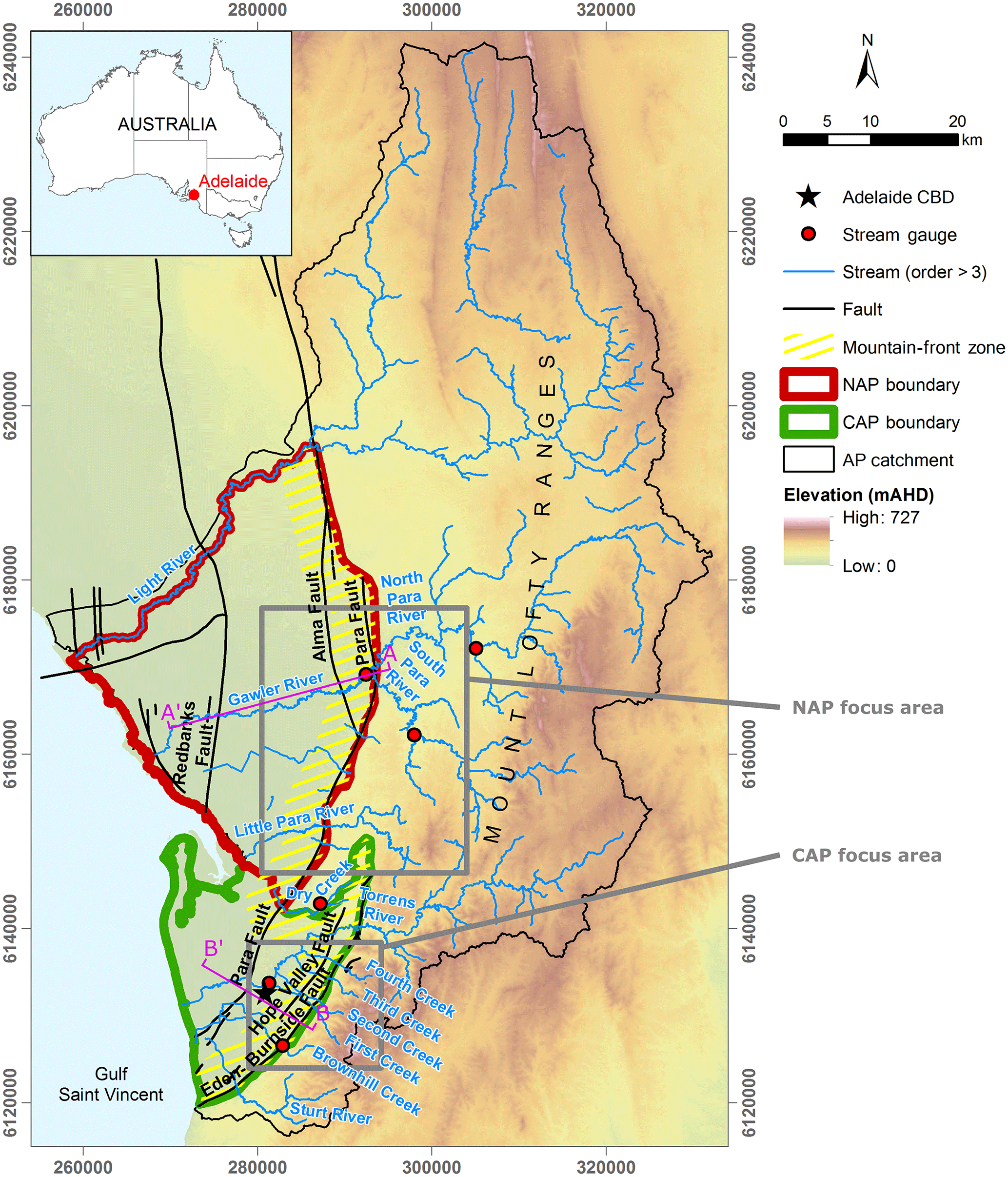
Figure 2 Situation map showing elevation (in metres according to the AHD, i.e. Australian Height Datum) and relevant features of this study.

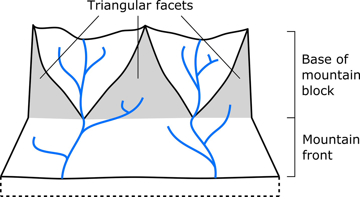
Figure 3 Schematic diagram showing triangular facets at the base of the mountain block (after Welch and Allen (2012)).

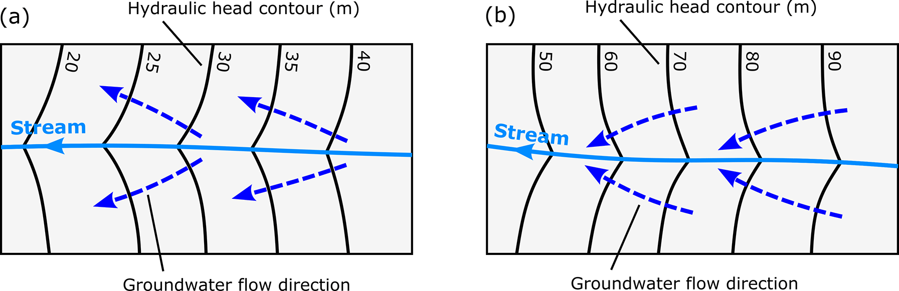
Figure 4 Schematic diagram showing hydraulic head contours and groundwater flow directions in the horizontal plane for (a) losing and (b) gaining stream conditions (after Winter et al. (1998)).

After presenting a general rationale for the use of hydraulic head, Cl⁻ and EC data to distinguish between MFR and MBR, the Adelaide Plains (AP) basin in South Australia (Fig. 2) is used as a case study to test the relevance of the approach. This semi-arid region features a sedimentary basin bounded by a mountain range – the Mount Lofty Ranges, from which most of the recharge is believed to be derived (Miles, 1952; Shepherd, 1975; Gerges, 1999; Bresciani et al., 2015a). Groundwater in this basin has been used for over a century for industry, water supply and agriculture. Nonetheless, and despite several recent studies, the relative contributions of MFR and MBR is still subject to debate. In particular, the hydraulic role of faults (i.e. acting as barrier or conduit to flow) that run along the mountain front remains unclear (Green et al., 2010; Bresciani et al., 2015a; Batlle-Aguilar et al., 2017). As a result of the common use of groundwater, a relatively high density of wells exists in the region, including in the mountain-front zone. Therefore, this case study provides a good example of the potential of the proposed approach.

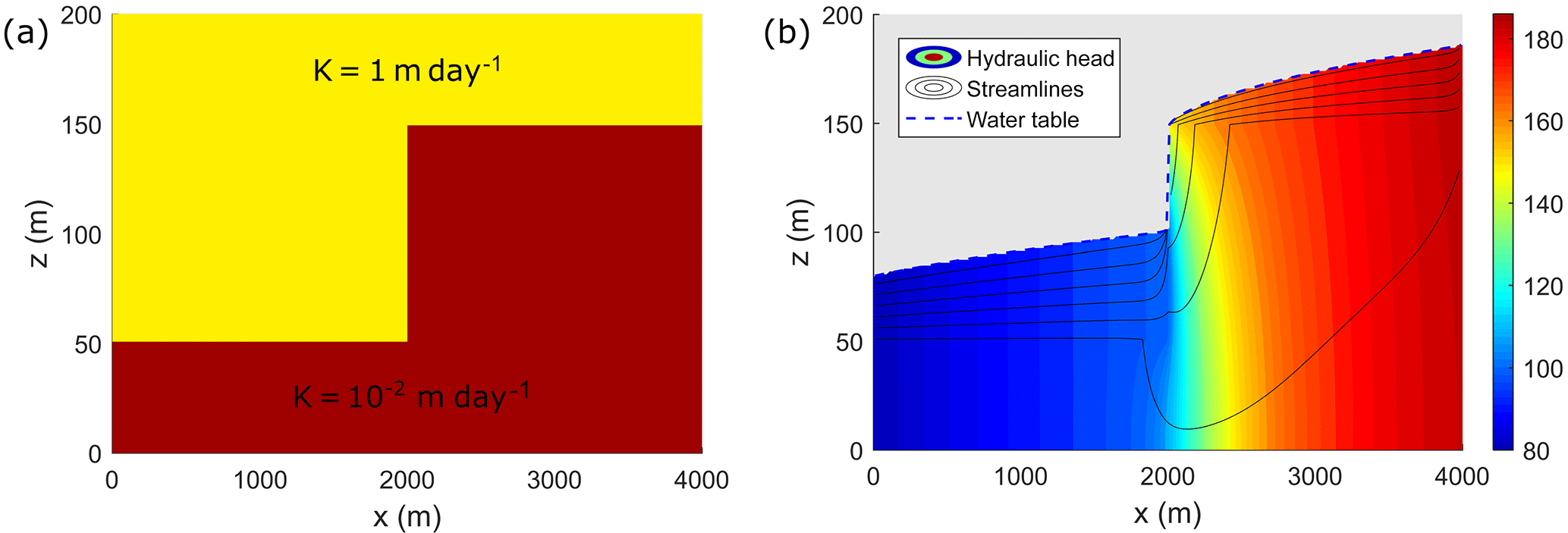
Figure 5 Impact of a difference in basement elevation induced as a result of faulting on hydraulic head in a hypothetical setting. (a) Hydraulic conductivity in a vertical cross section representing a sedimentary layer overlying a basement with significantly lower hydraulic conductivity, with the fault zone itself having no different hydraulic conductivity (i.e. the fault only implies the difference in basement elevation). (b) Results from an unconfined groundwater flow simulation in which a constant head (80 m) was specified on the left boundary and inflow was specified on the right boundary (at a rate proportional to the hydraulic conductivity). A sharp difference in hydraulic head is observed across the fault zone. The simulation was performed using MODFLOW-NWT (Niswonger et al., 2011), with 200 cells in horizontal direction and 150 cells in the vertical direction.

2 Rationale

In this section, a generic rationale is presented for the use of hydraulic head and Cl⁻ (or EC-derived Cl⁻) data to distinguish between MFR and MBR to basin aquifers. Hydraulic head and Cl⁻ data can be used independently, but as they are of different nature, it is expected that their simultaneous use will result in a more complete and reliable characterization of the recharge mechanisms.

2.1 Using hydraulic head

Hydraulic heads directly relate to groundwater dynamics. Consequently, hydraulic head patterns could theoretically enable the identification of groundwater flow paths, both in mountains and basins. Specifically, four types of analysis are suggested that could inform the likely occurrence or absence of MFR and MBR:

• Assessment of the correlation between hydraulic head and topography. In the mountain block, a good correlation would suggest that groundwater flow is dominated by local flow systems as opposed to regional flow systems (Tóth, 1963). This would imply that only a small portion of the recharge occurring over the mountain would make its way towards the basin. In fact, in this case MBR would be mostly limited to the recharge occurring over triangular facets in between stream catchments at the base of the mountain block (Fig. 3). Here, the recharge is less likely to be routed towards mountain streams, and instead it may be routed towards the basin (Welch and Allen, 2012). In the mountain-front zone, a good correlation between hydraulic head and topography would suggest that groundwater discharges to streams, so that MFR from stream leakage would be limited or non-existent.

• Analysis of the shape of hydraulic head contours adjacent to surface water features to identify losing and gaining stream conditions. It is well known that head contours show a curvature pointing in the downstream direction where the contour lines cross a losing stream (due to the mounding induced by groundwater recharge) (Fig. 4a), whereas they show a curvature pointing in the upstream direction where the contour lines cross a gaining stream (due to the depression induced by groundwater discharge) (Fig. 4b) (Winter et al., 1998). Performing such analysis in the mountain block should indicate whether mountain groundwater appears mostly routed towards local streams, which would make it less likely for MBR to be significant. Additionally, performing such analysis in the mountain-front zone should allow for testing the occurrence or absence of MFR in the form of stream infiltration, which is the predominant form of MFR (Wilson and Guan, 2004).

• Comparison of stream levels with nearby groundwater levels. A stream level higher than nearby groundwater levels would indicate a potential for stream infiltration, while the opposite would indicate a potential for groundwater discharge to stream. If the data density is low, this analysis may be preferable over the previous one (list item no. 2) as it does not require head contours to be accurately determined. However, it can only provide information on a potential interaction: groundwater discharge or recharge would be significant only if the hydraulic conductivity of the streambed is high enough. In contrast, the previous analysis (no. 2) could give a more definite answer, because the curvature of head contours at some distance from the stream should only be visible if the groundwater–surface water interaction is significant relative to other flow components (i.e. horizontal flow).

• Evaluation of the vertical head gradient in the mountain-front zone. Recharge areas are associated with a decrease in hydraulic head with depth, while discharge areas are associated with an increase in hydraulic head with depth (e.g. Wang et al., 2015). Hence, in the mountain-front zone, a head decrease with depth would suggest that MFR occurs (at a rate that depends on the vertical hydraulic conductivity of the aquifer). In contrast, an absence of head decrease (or a head increase) with depth would suggest that MFR does not occur.

In cases where faults run between the basin and the mountain, it may be tempting to study the difference in hydraulic head between the two sides of the fault zones. Intuitively, a large head difference would indicate that a fault zone constitutes a barrier to flow in the direction perpendicular to it (e.g. Bense et al., 2013), and consequently that MBR would be low. However, a large head difference across a fault zone may not always imply that the fault zone constitutes a hydraulic barrier. Let us consider the hypothetical case of a sedimentary layer overlying a basement of relatively low hydraulic conductivity and that features a sharp transition in elevation as a consequence of faulting (Fig. 5a). The hydraulic conductivity of the fault zone itself is assumed to be no different from that of the embedding materials (i.e. the fault only implies a difference in basement elevation). In this simple configuration, if the groundwater level right below the fault is lower than the basement elevation above the fault (as a result of downstream hydraulic controls), the groundwater level above the fault is essentially “disconnected” from the lower part (Fig. 5b). This is because in all cases, the groundwater level above the fault has to satisfy a minimum height (i.e. transmissivity has to be large enough) for groundwater to flow there. Hence, this example demonstrates that a large difference in head can exist across the fault zone despite the fault zone itself having no particularly low hydraulic conductivity. It should also be noted that regardless of the cause, the implications of a large difference in head, in terms of the amount of flow eventually crossing the fault zone, is far from obvious, as it depends on the hydraulic conductivity of the fault or the basement (which is in either case difficult to determine). A more relevant analysis may be to investigate whether or not the hydraulic head above of the fault is so high (relative to topography) as to imply that groundwater discharges locally to mountain streams instead of flowing across the fault towards the basin. In other words, what matters is the partitioning of the mountain groundwater between these two pathways. This is precisely what the first three types of analysis presented above should contribute to determining.

2.2 Using chloride

Chloride (Cl⁻) is a naturally occurring ion in groundwater that is generally considered as conservative in geochemical studies (Clark and Fritz, 1997). If there is no removal or addition of Cl⁻ in the aquifer, and if the effects of dispersion (i.e. mixing of water from different flow paths) can be neglected, the Cl⁻ concentration will be constant along each groundwater flow path (Bresciani et al., 2014). Under such conditions, if the potential MFR and MBR sources have a different Cl⁻ concentration, Cl⁻ could be an excellent tracer to distinguish between these two recharge mechanisms.

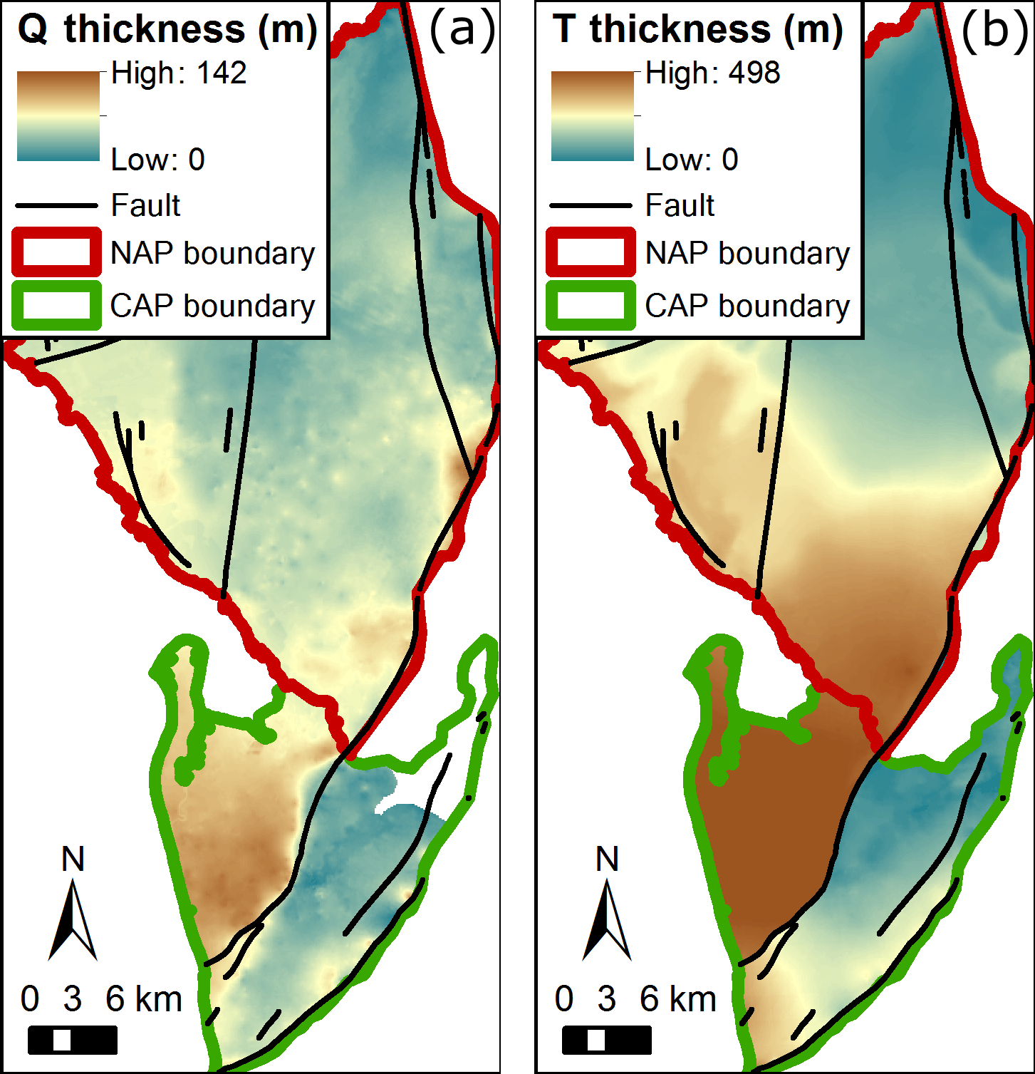
Figure 6 Total thickness of the Quaternary (Q) sediments (a) and Tertiary (T) sediments (b) in the AP basin. The colour schemes are different in (a) and (b).

In many cases, Cl⁻ in groundwater primarily originates from atmospheric deposition (Allison et al., 1994). The rate of atmospheric deposition depends on a number of factors including distance to the source (oceanic or terrestrial), elevation, terrain aspect, slope, vegetation cover and climatic conditions (Hutton and Leslie, 1958; Guan et al., 2010b; Bresciani et al., 2014). Other potential sources of Cl⁻ in groundwater include anthropogenic inputs (e.g. salting of roads, irrigation, application of fertilizer, leakage from septic/sewage systems) and dissolution of Cl-bearing minerals. Cl⁻ removal from solution is unlikely as Cl does not easily adsorb onto clays or precipitate as mineral (Clark and Fritz, 1997). The Cl⁻ concentration in recharge water also depends on evapotranspiration, which leaves Cl⁻ in solution, implying its enrichment (Eriksson and Khunakasem, 1969; Allison et al., 1994) (a growing vegetation could in theory counter this effect since Cl is a nutrient for plants (White and Broadley, 2001), but in practice the uptake of Cl from soil by most plant species is insignificant (Allison et al., 1994)). Thus, depending on how variable the above controlling factors are, the Cl⁻ concentration in mountain groundwater – i.e. the potential MBR source – may show significant spatial and temporal variability. The Cl⁻ concentration in stream water entering the basin – i.e. the potential MFR source – strongly depends on the streamflow generation mechanisms. If the mountain streams are supported by large proportions of overland flow or interflow, the Cl⁻ concentration in stream water entering the basin should tend to be lower than that in mountain groundwater, because these streamflow generation mechanisms imply relatively little evapotranspiration. In contrast, if the mountain streams are mostly supported by groundwater discharge, the Cl⁻ concentration in stream water entering the basin should tend to have an integrated value of the mountain groundwater concentration. In conclusion, while no general statement can be made, chances are that the potential MFR and MBR sources have a distinct Cl⁻ signature.

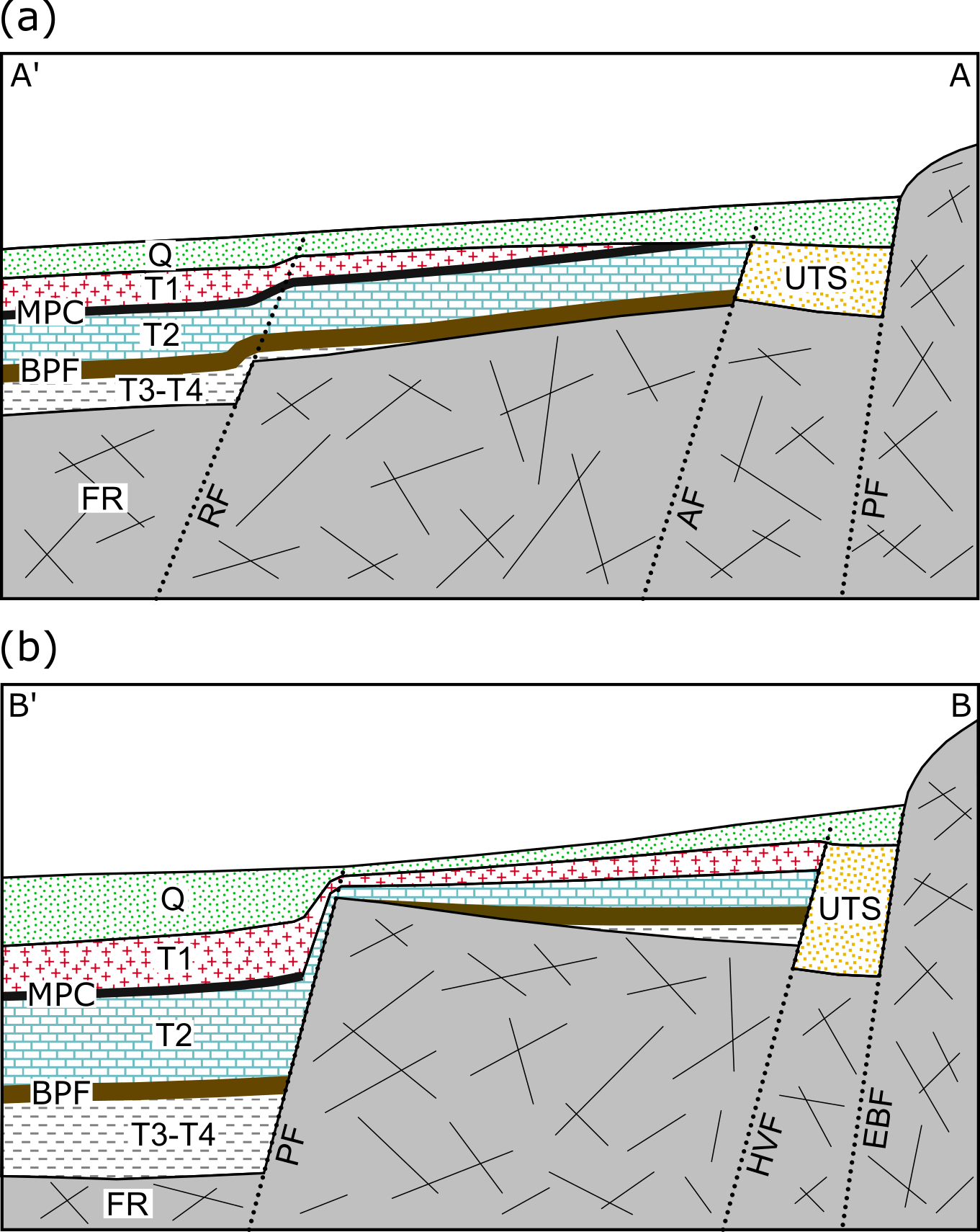
Figure 7 Schematic hydrogeological cross sections in (a) the NAP and (b) the CAP sub-basins (see Fig. 2) (after Shepherd, 1975; Gerges, 1999; Zulfic et al., 2008; Baird, 2010). Q: Quaternary aquifers (lumped together; in reality there are up to six different aquifers depending on location, separated by clay layers); T1, T2, T3 and T4: Tertiary aquifers; UTS: undifferentiated Tertiary sand aquifers; MPC: Munno Para clay aquitard; BPF: Blanche Point Formation aquitard; FR: fractured-rock aquifers; RF: Redbank Fault; AF: Alma Fault; PF: Para Fault; HVF: Hope Valley Fault; EBF: Eden–Burnside Fault.

In this study, the proposed strategy consists of analysing three types of water for Cl⁻: groundwater in the basin, groundwater in the mountain, and stream water in the mountain-front zone. Assuming steady-state concentrations and conservative Cl⁻, groundwater in the basin should have the same concentration as stream water in the mountain-front zone in the case of MFR (further assuming that transpiration from plants after stream infiltration and potential mixing with diffuse recharge are negligible), while it should have the same concentration as groundwater in the mountain in the case of MBR. As much as possible, the analysis should focus on comparing points that are not too far apart from one another and are along presumed flow paths, so as to reduce risks of misinterpretation caused by spatiotemporal variability in Cl⁻ concentration and dispersion. In particular, MBR should be most reliably assessed by comparing the groundwater Cl⁻ concentration in the uppermost part of the basin to that in the lowermost part of the mountain, along lines running perpendicular to the mountain front.

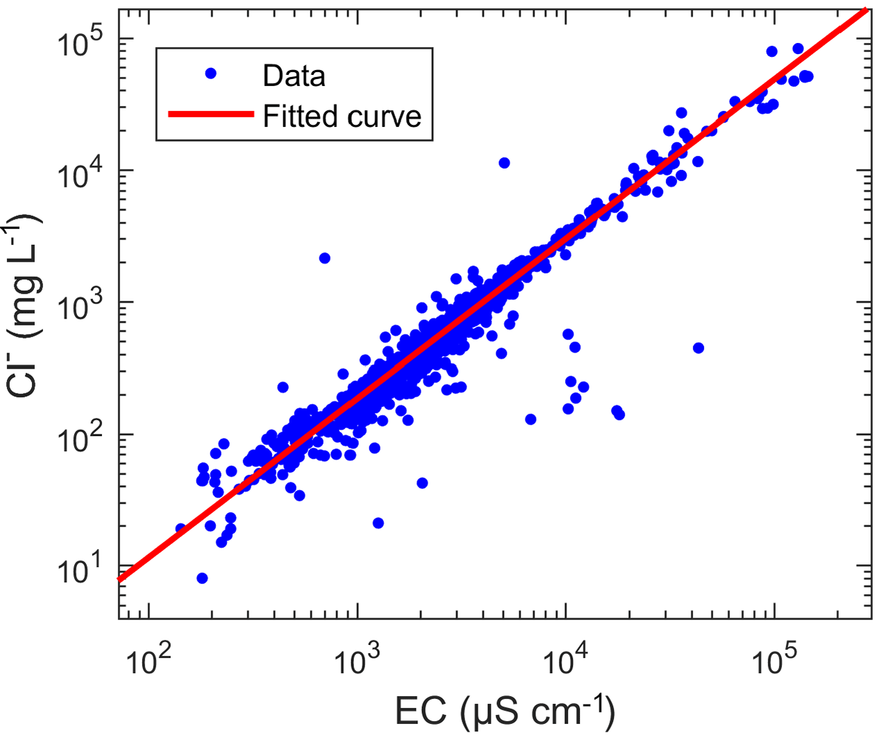
Figure 8 Cl⁻ versus EC data in the AP catchment. The fitted function used to describe the relationship is [Cl⁻] = 004411 × [EC]^1.208, where [Cl⁻] and [EC] are in units of milligrams per litre (mg L⁻¹) and microsiemens per centimetre (µS cm⁻¹), respectively (coefficient of determination: R²=0.9996).

Electrical conductivity values are known to be strongly correlated to Cl⁻ concentrations (Guan et al., 2010a). Therefore, EC data can be converted to Cl⁻ data if a relationship between the two can be assumed. Typically, EC is more routinely measured than Cl⁻, and thus this should significantly increase the dataset. Ideally, an empirical relationship between EC and Cl⁻ should be developed based on available pair measurements in the study area.

3 Case study

3.1 Study area and background

The Adelaide Plains basin is a coastal sedimentary embayment of 1700 km² in South Australia (Fig. 2). The area is bounded by the Mount Lofty Ranges to the east and south, by the Light River to the north, and by the Gulf Saint Vincent to the west. It can be split into two sub-basins: the central Adelaide Plains (CAP) sub-basin south of Dry Creek, and the northern Adelaide Plains (NAP) sub-basin north of Dry Creek. The topographic gradient is more pronounced in the CAP and adjacent mountains (regional slopes of about 0.8 and 7 %, respectively) than in the NAP and adjacent mountains (regional slopes of about 0.3 and 2.5 %, respectively). Torrens River and Gawler River are the largest rivers in the CAP and in the NAP, respectively. A number of streams run down from the Mount Lofty Ranges, either feeding these rivers or flowing directly into the ocean.

Figure 9 Hydraulic head and topographic contours in the NAP (a–b) and CAP (c–d) focus areas. On the basin side, (a) and (c) show the head in the Quaternary aquifers, while (b) and (d) show the head in the Tertiary aquifers. On the mountain side, all four sub-figures show the head in the Mount Lofty Ranges aquifers. In (a–b), the contour interval is 10 m in the basin and 40 m in the mountain (both for head and topography), while in (c–d), it is 20 m in the basin and 80 m in the mountain. Selected groundwater flow directions highlight apparent gaining stream conditions in the lower part of the mountain and loosing stream conditions in the mountain-front zone.

Precipitation is relatively low and potential evapotranspiration is high in this semi-arid area. The average rainfall is 445 mm yr⁻¹ (no snowfall) and the annual average maximum daily temperature of 21.6 ^∘C at Adelaide Airport station, located near the coast (station number 23034, 1970–2013; Australian Government, Bureau of Meteorology). Direct recharge from rainfall in the basin is thus expected to be relatively low. Instead, most of the recharge is believed to be derived from the adjacent Mount Lofty Ranges. The latter receive an average rainfall of 983 mm yr⁻¹ and negligible snowfall (i.e. only exceptionally and in insignificant quantities) at Mount Lofty Cleland Conservation Park (station number 23810, 1970–2013; Australian Government, Bureau of Meteorology), i.e. more than twice that of the basin. It also experiences cooler temperatures, with an annual average maximum daily temperature of 15.2 ^∘C at Mount Lofty (station number 23842, 1993–2007; Australian Government, Bureau of Meteorology). The majority (77 %) of the rainfall in the Mount Lofty Ranges occurs during autumn and winter (May–September) (station number 23810, 1970–2013), suggesting a strong seasonality of the recharge.

The basin comprises complex, spatially dependent sequences of Quaternary and Tertiary sedimentary deposits (Gerges, 1999). The Quaternary sediments are dominated by fluvio-lacustrine clay interbedded with sand and gravel. The Tertiary sediments are dominated by sand, sandstone, limestone, chert, marl and shell remains interbedded with clay. A number of faults dissect the basin. Among these, the Eden–Burnside Fault and the Para Fault are of primary interest in this study since these faults run along the foothill, almost at the margin of the CAP and the NAP sub-basins, respectively (Fig. 2). The total thickness of the sedimentary units increases sharply on the downthrown side of the major faults (up to 400 m in places). The thickness of the Quaternary sediments ranges from 0 to about 140 m across the basin (Fig. 6a), while that of the Tertiary sediments ranges from 0 to about 500 m (Fig. 6b). The Tertiary sediments are directly outcropping in the northeast part of the CAP. The basement of the basin and the Mount Lofty Ranges are mostly comprised of Proterozoic fractured rocks of various lithologies including slate, phyllite, quartzite, limestone and dolomite. Superficial sedimentary deposits (typically less than 20 m in thickness) also exist locally in the Mount Lofty Ranges.

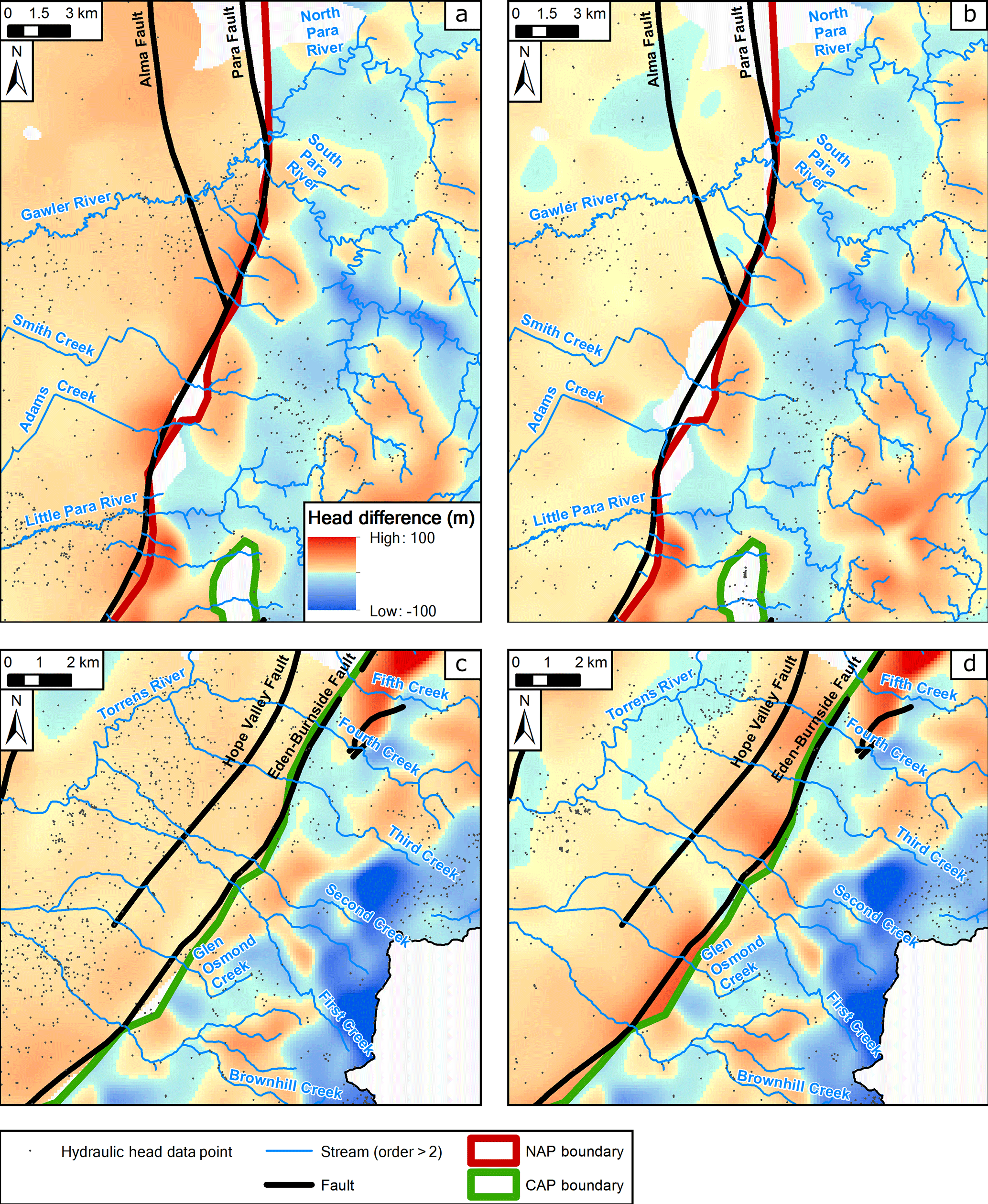
Figure 10 Head difference in the NAP (a–b) and CAP (c–d) focus areas. On the basin side, (a) and (c) show the nearest river head (approximated by topography) minus the head in the Quaternary aquifers, while (b) and (d) show the head in the Quaternary aquifers minus the head in the Tertiary aquifers. On the mountain side, all four sub-figures show the nearest river head minus the head in the Mount Lofty Ranges aquifers. The same colour scheme is applied everywhere and is indicated in (a). Reddish colours are for positive values, indicating a potential for downward flow (i.e. groundwater recharge). Blueish colours are for negative values, indicating a potential for upward flow (i.e. groundwater discharge).

Up to six semi-confined aquifers (named Q1 to Q6) are recognized within the Quaternary sediments from the central to western side of the basin (Gerges, 1999) (i.e. downstream of the mountain-front zone). These aquifers contain water of variable salinity with a median value of around 1300 mg L⁻¹. The underlying Tertiary sediments are generally subdivided into four aquifers (named T1 to T4) over a large part of the basin. However, there is no clear hydrogeological distinction between the various Tertiary sediments along most of the mountain front in both sub-basins, and thus in this area they are considered to form a single undifferentiated Tertiary aquifer (Gerges, 1999; Zulfic et al., 2008; Baird, 2010). Simplified cross sections of the aquifers in the NAP and CAP sub-basins are shown in Fig. 7a and b, respectively. Salinity is relatively low in the upper aquifer (T1) with a median value of around 600 mg L⁻¹, slightly higher in the T2 aquifer with median values of around 1000 mg L⁻¹, and significantly higher in deeper aquifers with median values of 8400 and 40 000 mg L⁻¹ in T3 and T4, respectively (but note that very few data are available from the latter two aquifers). Because they present large areas of good salinity and yield, the T1 and T2 aquifers have been used since 1914 for occasional water supply, irrigation and industrial activities and are currently the main targets of groundwater extraction in the AP (Gerges, 1999; Zulfic et al., 2008). Long-term, large cones of depression in both of these aquifers and forecasted increases in groundwater demand raise concerns about the sustainability of extraction in the coming years (Bresciani et al., 2015a). Risks are related to both potential depletion of the resource and rise in salinity from the migration of higher-salinity groundwater, which could make groundwater unusable. To better assess these risks, a thorough understanding of the recharge mechanisms to these aquifers is necessary.

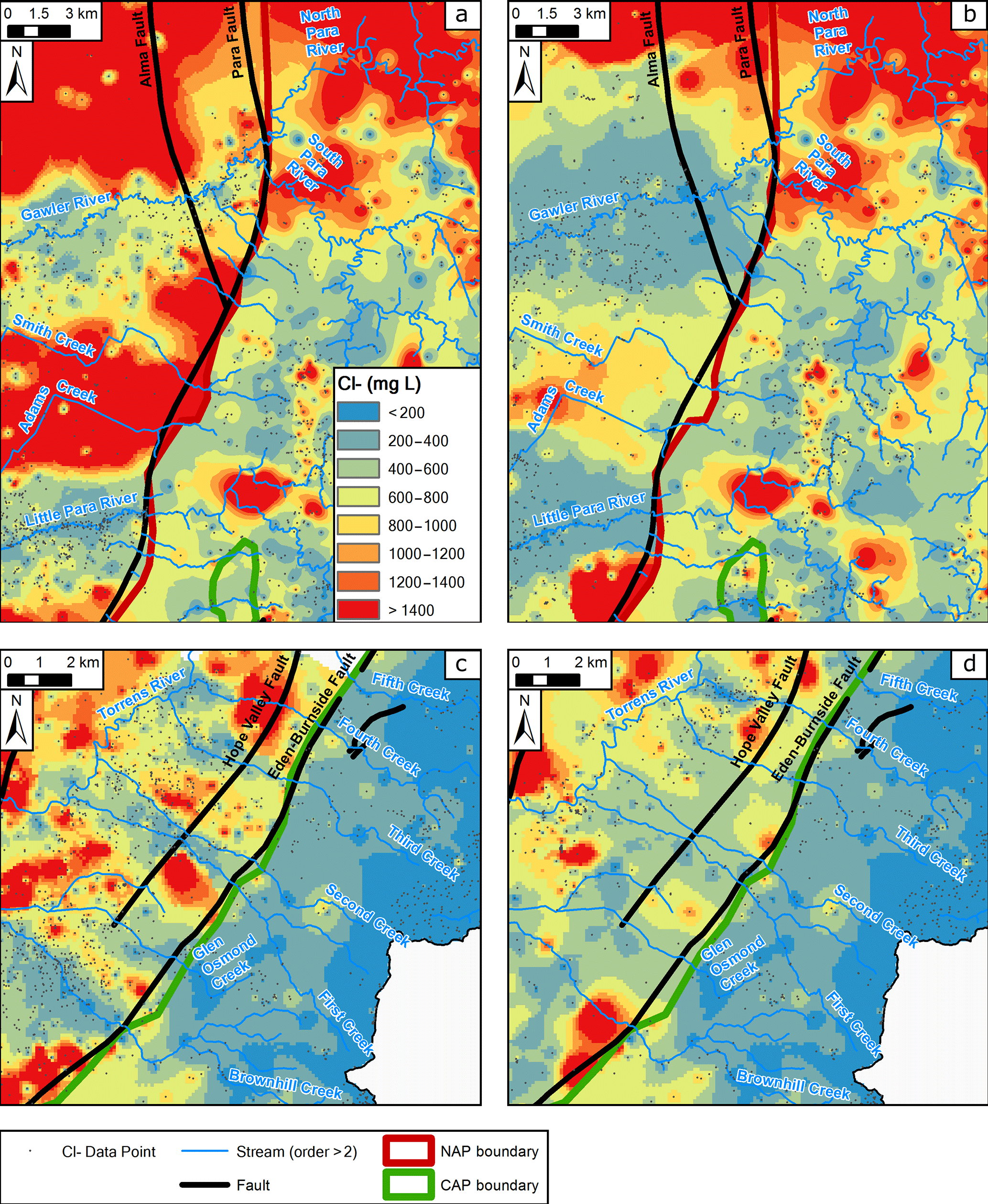
Figure 11 Cl⁻ concentration in the NAP (a–b) and CAP (c–d) focus areas. On the basin side, (a) and (c) show the Cl⁻ concentration in the Quaternary aquifers, while (b) and (d) show the Cl⁻ concentration in the Tertiary aquifers. On the mountain side, all four sub-figures show the Cl⁻ concentration in the Mount Lofty Ranges aquifers. The same colour scheme is applied everywhere and is indicated in (a). The latter is chosen to be favourable to the study of relatively low-salinity zones; i.e. all Cl⁻ concentrations larger than 1400 mg L⁻¹ are included in the same class (red colour), but in reality much higher values exist.

Early investigations suggested that the natural (i.e. pre-development) recharge to the Tertiary aquifers of the basin was dominated by stream infiltration along the mountain front (i.e. MFR) (Miles, 1952; Shepherd, 1975). In contrast, subsequent investigations suggested that the natural recharge of the Tertiary aquifers was dominated by subsurface flow from the Mount Lofty Ranges (i.e. MBR) (Gerges, 1999, 2006). The latter conceptual model has formed the basis of most investigations of the Tertiary aquifers since its presentation and has underpinned the development of a number of groundwater flow and transport models of the basin aquifers (Jeuken, 2006a, b; Zulfic et al., 2008; Baird, 2010; Georgiou et al., 2011; Bresciani et al., 2015b). However, studies from Green et al. (2010) and Bresciani et al. (2015a) produced results supporting the hypothesis that MFR could also be significant. To further investigate this question, the present study provides a re-appraisal of available hydraulic head, Cl⁻ and EC data through application of the above rationale.

3.2 Datasets

3.2.1 Hydraulic head dataset

Hydraulic head data in the AP catchment (i.e. the area including both the basin and contributing mountain areas based on surface topography) were retrieved from the WaterConnect database (http://www.waterconnect.sa.gov.au, Government of South Australia) on 4 November 2016. The collection dates span more than a century, the earliest measurements being from 1906 and the latest from 2016. The data were filtered out for unsuitable measurements such as measurements taken during pumping, aquifer testing or drilling. After filtering, 111 538 hydraulic head measurements from 9561 wells were obtained.

The data were subsequently split according to three aquifer groups: the AP Quaternary aquifers, the AP Tertiary aquifers (“AP” in these expressions will be omitted in the remaining text) and the Mount Lofty Ranges aquifers. This grouping is relevant in view of the hydrogeological characteristics of the system and the objective of the study. In particular, we did not distinguish between the T1 and T2 aquifers (i.e. the two main aquifers of the AP basin) because, as mentioned earlier, they are undifferentiated along most of the mountain front. In the Mount Lofty Ranges, the presence of complex fracture networks and high relief can induce the blurring of otherwise depth-dependent hydraulic signals, and so splitting the data according to depth in this area may not be very meaningful and it would reduce data density. The name of the aquifer into which the wells were screened was informed in the database for about two-thirds of the wells (6209). This allowed for assignment of these wells to one of the above aquifer groups. For the remaining one-third of wells, the aquifer group for the wells located in the basin was determined by comparing the well mid-screen elevation to the bottom elevation of the Quaternary sediments and to the top elevation of the basement. The largest number of wells was from the Quaternary aquifers (3964), followed by the Mount Lofty Ranges aquifers (3589) and the Tertiary aquifers (1768). Wells screened into the basement of the basin were disregarded (240 wells).

Groundwater-level fluctuations can be an issue for data interpretation. In particular, as this study focuses on natural recharge mechanisms, the impact of pumping constitutes a potentially important bias. It should be noted that the density of hydraulic head data is higher in areas of lower groundwater salinity, which coincides with areas that have experienced greater changes due to pumping. The measurements made before the main development period (i.e. before 1950) may have been less affected by pumping than more recent measurements, but limiting the analysis only to these measurements would dramatically reduce the data density. In addition, even the earliest measurements may not be free of pumping influence, since it is likely that these were precisely taken to monitor the impact of pumping. Hence, instead of subjectively fixing an arbitrary date beyond which the data would be excluded, all data were retained regardless of the measurement date. For each of the wells that had multiple measurements, the temporal mean hydraulic head was calculated in an effort to smooth out the measurement errors and temporal fluctuations. The analysis focuses on these mean values.

3.2.2 Chloride dataset

Groundwater Cl⁻ data in the AP catchment were also retrieved from the WaterConnect database on 4 November 2016. This dataset was extended using the more commonly available EC data from the database. A strong relationship between EC and Cl⁻ was found from 1,559 pair measurements (R²=0.9996, Fig. 8). In wells where only EC data were available, EC values were converted into Cl⁻ concentrations using this relationship. In total, 34 145 Cl⁻ or EC-converted Cl⁻ data (simply referred to as Cl⁻ data) from 12 660 wells were obtained (i.e. slightly more than for hydraulic heads, partly due to a less-restrictive filtering, i.e. keeping measurements taken during pumping or aquifer testing). The collection dates span the same period as for the hydraulic head data.

The Cl⁻ data were subsequently split according to the same three aquifer groups as indicated above for the hydraulic head data. The same procedure was also applied to determine the aquifer group to which the wells belong. The largest number of wells was from the Quaternary aquifers (4963), followed by the Mount Lofty Ranges aquifers (4395) and the Tertiary aquifers (2963).

Pumping may also have impacted Cl⁻ concentrations by inducing migration of the original groundwater, whose concentration is spatially variable (although this effect may be seen later than on hydraulic heads since solute travel times are typically longer than pressure travel times). Also, as for hydraulic head data, the density of Cl⁻ data is higher in areas that have experienced pumping. Additionally, in the uppermost aquifers, irrigation may have locally influenced the Cl⁻ concentration. Nonetheless, following the same reasoning as for hydraulic heads, all available Cl⁻ data were retained regardless of the measurement date. For each of the wells that had multiple measurements, the temporal mean Cl⁻ concentration was calculated. The analysis focuses on these values.

Table 1 Surface water flow rate, EC values and their conversion into Cl⁻ concentrations for the six gauging stations located near the mountain-front zone (gauging station number in parenthesis; see Fig. 2 for site locations). Note that the North Para River and South Para River join about 1 km downstream of the Para Fault to form the Gawler River.

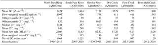
Flow rate and EC data from streams running down from the Mount Lofty Ranges into the AP basin were also retrieved from the WaterConnect database. Six gauging stations were located close enough to the mountain front to be relevant to the current study. Details on this dataset are given in Table 1. The reported EC values of surface water were converted into Cl⁻ concentrations using the same relationship as that developed for groundwater. This approach is deemed appropriate given the common origin of these waters, even though potentially different chemical reactions might slightly affect the relationship.

3.3 Data analysis

Given the relatively large area investigated, the analysis presented below concentrates on two “focus areas” that cover the transition between the Mount Lofty Ranges and the AP basin: one at the margin of the NAP sub-basin and one at the margin of the CAP sub-basin (locations indicated in Fig. 2). Figures for the entire study area are also available in the Supplement (Figs. S1–S12). These do not call for a different interpretation.

3.3.1 Hydraulic heads

Hydraulic head maps were constructed for the three aquifer groups (Quaternary aquifers, Tertiary aquifers and Mount Lofty Ranges aquifers) (Figs. 9, 10). In constructing these maps, the choice of the interpolation method and associated parameters revealed to be critical. The classical inverse distance weighting method would produce the well-known “bull's eye” effect around individual data points. This could severely compromise the interpretation of head contours. Instead, the diffusion kernel interpolation method from the Geostatistical Analyst extension of ArcGIS 10.4.1 was used. This method allows for a more realistic interpolation when the underlying phenomenon governing the data is diffusive, as is the case for hydraulic heads. The most important parameter in this method is the bandwidth, which is used to specify the maximum distance within which data points are used for prediction. Making this parameter too small would undermine the prediction capability as many areas would remain uncovered by the interpolation, while making it too large would produce overly smoothed results. A good compromise was found by setting this parameter to 1200 m for the NAP focus area and to 800 m for the CAP focus area – reflecting a higher density of streams and data in the latter case. Topographic contours were also constructed. To facilitate the comparison with head contours, these were created after application of a circular moving-average window to the topography using a radius that matches the bandwidth used in the interpolation method for hydraulic head (i.e. 1200 m in the NAP focus area and 800 m in the CAP focus area).

Figure 9a displays hydraulic head and topographic contours in the NAP focus area, showing the Quaternary aquifers on the basin side and the Mount Lofty Ranges aquifers on the mountain side. The results are quite contrasted between the mountain and the basin. In the mountain, head contours follow the topographic contours relatively closely, and their shape is most often indicative of gaining stream conditions. Note that one should not expect to see sharp “V” shapes where head contours cross streams (i.e. as in Fig. 4) due to the limited data density. Instead, head contours are smoothly curved. In the basin, head contours do not closely follow the topographic contours, and their shape is generally indicative of losing stream conditions (especially close to the basin margin). Figure 9b also displays hydraulic head and topographic contours in the NAP focus area, but showing the Tertiary aquifers on the basin side instead of the Quaternary aquifers (on the mountain side, this figure is identical to Fig. 9a). Head contours in the Tertiary aquifers are generally indicative of focused recharge along streams, but on a somewhat larger scale, i.e. showing wider curvatures than in the Quaternary aquifers (mostly around Gawler River and Little Para River). Figure 9c and d display analogous results for the CAP focus area. Similar to above, in the mountain, head contours are relatively well correlated with topographic contours and their shape is generally indicative of gaining conditions. In the basin, head contours in the Quaternary aquifers are not very distinct from topographic contours, but nevertheless tend to indicate losing rather than gaining stream conditions close to the basin margin (Fig. 9c). In the Tertiary aquifers, head contours are quite distinct from topographic contours and are quite clearly indicative of focused recharge along a majority of streams (Fig. 9d). Near Glen Osmond Creek and Brownhill Creek, groundwater flow predominantly appears oriented towards the southwest, which may result from the bedrock sloping in this direction (the Tertiary sediment thickness can be seen to increase in Fig. 6b).

Figure 10a–d display the difference, in every point, between river head (approximated by the topographic elevation of the nearest river) and groundwater head. Figure 10a shows the NAP focus area, with the Quaternary aquifers on the basin side and the Mount Lofty Ranges aquifers on the mountain side. In the mountain, the results generally reveal a potential for gaining stream conditions along large portions of the main rivers (i.e. North Para River, South Para River and Little Para River). Potential losing stream conditions are indicated around the upper reaches of streams, suggesting that these are not supported by groundwater discharge, but are rather initiated by overland flow or interflow. This observation is consistent with the fact that most of the stream headwaters in the Mount Lofty Ranges are ephemeral. Potential losing stream conditions are also observed locally around a few streams in the lowest part of the Mount Lofty Ranges (e.g. South Para River and Smith Creek). This observation is not in line with the interpretation of head contours made from Fig. 9a, and this inconsistency might be an artefact of the temporal averaging of hydraulic heads, i.e. the hydraulic heads might be on average lower than the river head but the stream might still be gaining due to important groundwater discharge in some periods (but this explanation remains a hypothesis). In the basin, the Quaternary aquifers are revealed as potentially receiving water from streams everywhere, and especially close to the basin margin where the head difference is the largest. Figure 10b shows the head difference between the Quaternary aquifers and the Tertiary aquifers on the basin side, such as to investigate the vertical connection between these aquifers (on the mountain side, this figure is identical to Fig. 10a). The hydraulic head appears larger in the Quaternary aquifers than in the Tertiary aquifers over most of the area. This indicates a potential for downward groundwater leakage from the Quaternary aquifers to the Tertiary aquifers. The rate at which this leakage occurs is nonetheless difficult to estimate, since it is also a function of the effective vertical hydraulic conductivity and vertical distance between these units, which are largely unknown. Similar observations and interpretations can be made of the CAP focus area (Fig. 10c, d).

Most observations from Figs. 9 and 10 suggest that groundwater flow is dominated by local flow systems in the Mount Lofty Ranges. This indicates that only a small proportion of the recharge occurring over the mountain may make its way towards the basin. Hence, if MBR occurs, it would be probably limited to the routing of the recharge occurring over triangular facets in between stream catchments at the base of the mountain (see Sect. 2.1). Moreover, the results generally suggest that MFR through stream leakage is an important recharge mechanism for both the Quaternary aquifers and the Tertiary aquifers of the AP basin.

3.3.2 Chloride concentrations

Cl⁻ concentration maps were also constructed for the three aquifer groups (Quaternary aquifers, Tertiary aquifers and Mount Lofty Ranges aquifers) (Fig. 11). Here the inverse distance weighting interpolation method from the Geostatistical Analyst extension of ArcGIS 10.4.1 was used. This method is appropriate for Cl⁻ because its analysis does not especially make use of the shape of concentration contours, and hence the bull's eye effect is not really an issue. Furthermore, Cl⁻ cannot be assumed to result from a diffusive process since advection is expected to dominate on the scale of this study, and so the diffusive kernel method would be inappropriate. The inverse distance weighting interpolation method also has the advantage of being exact at the data points. The power parameter was set to 2, and a standard neighbourhood was used with 15 maximum neighbours and 10 minimum neighbours. The same parameters were used for both NAP and CAP focus areas.

Figure 11a shows the Cl⁻ concentrations in the Quaternary aquifers and the Mount Lofty Ranges aquifers in the NAP focus area. This figure reveals a strong correlation between low Cl⁻ concentration zones and the location of the main rivers in the basin (Gawler River and Little Para River). It seems unlikely that such a correlation would be observed if MBR was the main recharge mechanism. By contrast, no obvious correlation can be found in the mountain. Here, the Cl⁻ concentration mostly appears correlated with elevation, with lower values occurring at higher elevations. This trend is expected, since the rate of evapotranspiration – which largely controls Cl⁻ concentration – is expected to decrease with elevation as a result of higher rainfall and lower temperature. In line with these observations, there is a clear discontinuity in Cl⁻ concentration at the transition between the mountain and the basin almost everywhere along the mountain front. This suggests that little or no hydraulic connection occurs between the mountain and the basin through the subsurface (i.e. MBR is probably insignificant). Similar observations hold in Fig. 11b, where the Tertiary aquifers are shown in the basin instead the Quaternary aquifers. The zones of low Cl⁻ concentration around Gawler River and Little Para River are wider in these aquifers than in the Quaternary aquifers, which is consistent with the above observation that the head contours display a wider curvature around these rivers. Figure 11c and d show analogous results for the CAP focus area. The Cl⁻ concentration is generally lower than in the NAP focus area, especially in the mountain, most likely a result of lower evapotranspiration associated with the higher elevation of this area. A strong correlation between zones of low Cl⁻ concentration and stream locations can also be seen in the basin. These zones appear wider and somewhat less distinct in the Tertiary aquifers than in the Quaternary aquifers, but it should be noted that the data density is lower in these aquifers. In both cases, as in the NAP, a sharp change in Cl⁻ concentration can be seen at the transition between the mountain and the basin, therefore suggesting that MBR is insignificant.

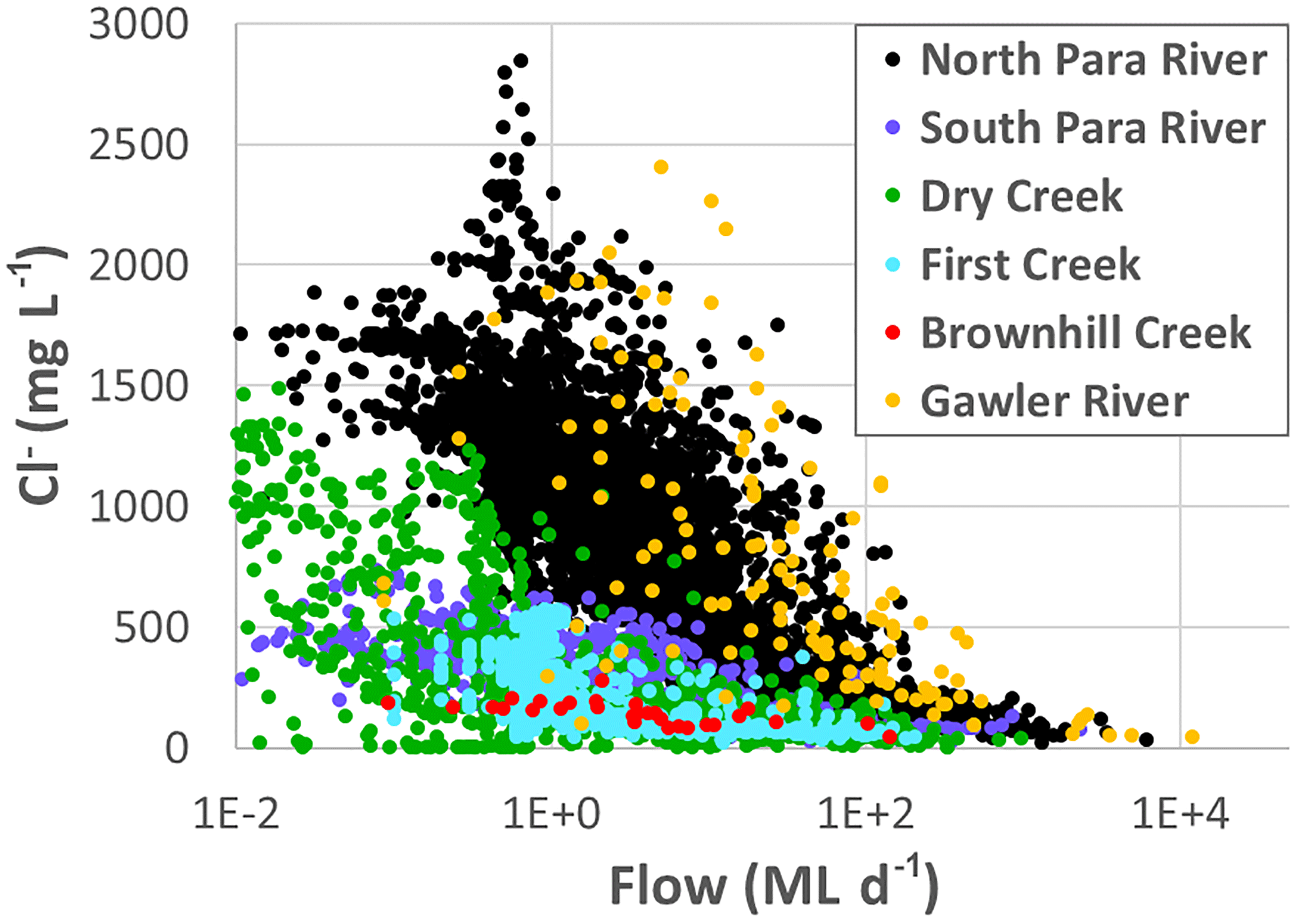
Figure 12 Scatter plot of chloride concentration versus streamflow rate for six streams running down from the Mount Lofty Ranges into the AP basin.

The Cl⁻ concentration in streams running down from the Mount Lofty Ranges into the AP basin was analysed to investigate whether stream leakage can explain the groundwater Cl⁻ concentrations measured in the basin. A summary of available flow rate, electrical conductivity and derived Cl⁻ concentration data for six monitoring stations located near the transition between the mountain and the basin is presented in Table 1. The location of the stream gauges is indicated in Fig. 2. The relationship between streamflow rate and Cl⁻ concentration is shown from a scatter plot in Fig. 12. The stream Cl⁻ concentration displays significant variations, with a decreasing trend as flow increases. The relationship between flow rate and Cl⁻ concentration nevertheless varies between different streams. This probably reflects different catchment characteristics that are likely to influence the streamflow generation mechanisms (i.e. topography, climate, geology, land use). The variations of streamflow rate and Cl⁻ concentration show a strong seasonality, as illustrated through selected time series for Gawler River and Brownhill Creek in Fig. 13a and b, respectively. These time series show that the periods of low Cl⁻ concentration and high flow coincide with the wet season (May–September). During this season, lower Cl⁻ concentrations in stream water can be explained by a relatively large contribution of overland flow or interflow to streamflow generation, as these processes should experience little evapotranspiration relative to subsurface flow contribution. The significance of overland flow or interflow is also supported by observations mentioned above. During high flow periods, the infiltration potential in the mountain-front zone should be enhanced due to higher stream water levels and wider wetted areas. We therefore propose to estimate a representative value of the MFR Cl⁻ concentration by calculating the flow-weighted average Cl⁻ concentration in stream water. A more rigorous approach would require knowledge of the timing and rate of stream leakage, which are not available. The flow-weighted average Cl⁻ concentration is 221, 115, 146, 67, 107 and 91 mg L⁻¹ in the North Para River, South Para River, Gawler River, Dry Creek, First Creek and Brownhill Creek, respectively (Table 1). These data show that streams are a plausible source for the low Cl⁻ concentrations observed in the basin aquifers (Fig. 11).

4 Discussion

4.1 Strengths and limitations of using hydraulic head and chloride data

One of the main strengths of hydraulic head data is that they can indicate the contemporary flow direction (if hydraulic conductivity can be considered to be isotropic). In this study, the analysis of head contours suggested that groundwater in the Mount Lofty Ranges discharges to local streams for a large part. It also allowed for the identification of losing stream conditions in the mountain-front zone, where leakage from streams appears to recharge not only the Quaternary aquifers but also the deeper Tertiary aquifers. Studying the head variation with depth in the basin gave further evidence that groundwater flows from the Quaternary aquifers to the underlying Tertiary aquifers, even though the rate of this flow is unknown.

The main limitation of hydraulic head data is probably that these data are quite sensitive to pumping. This is problematic when the objective is to study the natural (i.e. pre-development) recharge mechanisms. Pumping in the AP basin mostly affects groundwater levels in the western part of basin, where large cones of depression exist in the Tertiary aquifers due to extensive historical and ongoing pumping (Bresciani et al., 2015a). Therefore, for the purpose of this study, which focuses on the eastern part of the basin (where the mountain-front zone is located), this issue may not be as critical. However, smaller-scale pumping wells surely also exist in the mountain-front zone and in the mountain, and may affect the results to an unknown degree. This represents a non-negligible source of uncertainty.

Cl⁻ is potentially an effective tool to distinguish between MFR and MBR. But for this, the stream water Cl⁻ concentration in the mountain-front zone (i.e. a potential MFR source) needs to be significantly different from the groundwater Cl⁻ concentration at the base of the mountain (i.e. potential MBR source). Different processes involved in the generation of MFR and MBR imply that these two potential sources of water may indeed have different Cl⁻ concentrations (see Sect. 2.2). This is certainly the case in the present case study, where the Cl⁻ concentration at the base of the mountain is seen to be significantly different from that of the basin, thereby suggesting that MBR is insignificant. In contrast, the Cl⁻ concentration in streams appears to be similar to that of the low Cl⁻ concentration zones of the basin, which are aligned with surface water features. These observations leave little doubt regarding the recharge mechanisms in the AP basin, i.e. MFR appears to be the dominant recharge mechanism.

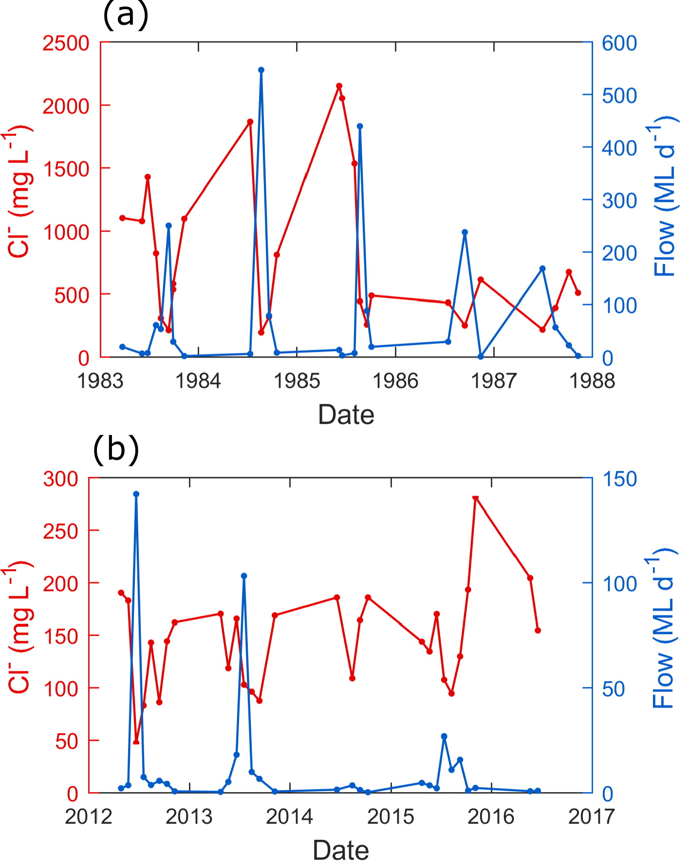
Figure 13 Stream water chloride concentration and flow rate over selected periods for (a) Gawler River and (b) Brownhill Creek. The axes in (a) and (b) have a different scale.

As for hydraulic heads, pumping can potentially distort the Cl⁻ concentrations from those of the natural system. In addition, irrigation may influence the Cl⁻ concentration in shallow wells located in agricultural areas. However, changes in solute concentrations are expected to be observed later than hydraulic head changes, and a dramatic shift in Cl⁻ concentrations is unlikely to be seen in Cl⁻ concentrations away from the main areas of pumping. Furthermore, if recharge from streams in the basin was only a result of recent pumping, groundwater should have a very modern (i.e. post-development) recharge signature. Groundwater dating shows that this is not the case (Batlle-Aguilar et al., 2017). It can also be noted that the correlation between the zones of low groundwater salinity and stream locations was already observed in the 1950s, i.e. using measurements anterior to the main development period (Miles, 1952).

The interpretation of Cl⁻ data also relies on the assumptions of constant Cl⁻ inputs. This assumption is widely accepted in the literature for hydrogeological studies and in applications of the chloride mass balance method to estimate recharge (Wood, 1999; Scanlon et al., 2006; Crosbie et al., 2010; Healy and Scanlon, 2010). This assumption may not be strictly satisfied over the AP basin because groundwater in the Tertiary aquifers can be quite old, as revealed by numerous samples showing paleo-meteoric origin (>12 000 years) according to carbon-14 dating and noble gas measurements (Batlle-Aguilar et al., 2017). This indicates that different climatic conditions may have prevailed at the time of recharge, implying possible variations in Cl⁻ inputs. However, such old groundwater is mostly observed in the western part of the basin. Groundwater in the mountain-front zone is younger (in most cases <10 000 years according to carbon-14 dating), making it less likely for these to reflect drastically different paleo-climatic conditions. Furthermore, even if the Cl⁻ inputs did vary over time, such temporal variation would not in itself explain the correlation of groundwater Cl⁻ concentration with stream locations in the basin.

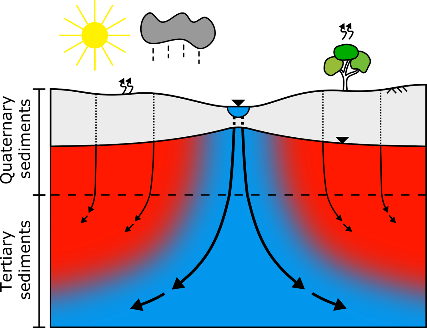
Figure 14 Conceptual model of the recharge mechanisms for the aquifers of the AP basin, as seen in a cross section perpendicular to a stream in the mountain-front zone, and how these mechanisms can explain the observed groundwater salinity. Blue to red colours indicate relatively low to high salinity.

Finally, the assumption of conservative Cl⁻ is deemed reasonable in view of the geology of the study area, which is not known to bear evaporite deposits such as halite. This assumption was also tested by analysing the chloride ∕ bromide (Cl⁻ ∕ Br⁻) ratio from 161 well samples distributed over the study area. The average Cl⁻ ∕ Br⁻ ratio from these samples is 739 $+/-$ 173 (molar) (Fig. S13). This shows that groundwater has a similar Cl⁻ ∕ Br⁻ ratio to seawater (∼ 650 molar), hence indicating that there is little water-rock interactions or dissolution of evaporite deposits (Drever, 1997; Davis et al., 1998). The low variance of the Cl⁻ ∕ Br⁻ ratio also suggests that the dominant process for the increasing salinity in the groundwater is evapotranspiration (Cartwright et al., 2006). Furthermore, even if Cl⁻ was not strictly conservative, focused recharge from streams in the basin would again appear necessary to explain the fact that the zones of low groundwater Cl⁻ concentration are found along streams.

Compared to other methods that use noble gas, radioactive or isotopic tracers, the above approach appears simpler, more cost effective and more reliable due to the much higher data density generally achievable (i.e. given current technologies and budget constraints). Nevertheless, in contrast with some other methods (e.g. noble gases), it should be noted that this approach is only qualitative. I.e. it does not allow for the quantification of the relative proportion of MFR and MBR and their absolute rate. One way to extend the ideas presented in this study to gain more quantitative insight would be to use the data as calibration targets in a groundwater flow and Cl⁻ transport model. This is also the subject of ongoing efforts (Bresciani et al., 2015b).

4.2 MFR versus MBR in the AP basin

In an early study, Miles (1952) noted that the pre-development groundwater levels along the mountain front of the AP basin were reflective of unconfined conditions, and that the subsurface materials in this zone were favourable to stream infiltration. In addition, Miles (1952) already analysed the groundwater salinity distribution. He observed that salinity contours were forming fan-shaped zones of low-salinity “mushrooming” outwards from streams, with such patterns being visible up to more than 100 m below the ground surface. He concluded that stream infiltration in the mountain-front zone was a major recharge mechanism for the basin aquifers. Later, in a study of the NAP aquifers, Shepherd (1975) arrived at the same conclusion, partly using similar arguments and further noting that (i) groundwater hydrographs in the Quaternary aquifers were each year showing a rapid rise in water level shortly after Gawler River and Little Para River started to flow, and (ii) the vertical head gradient and vertical hydraulic conductivity were indicative of significant downward flow from the Quaternary to the Tertiary aquifers. Additionally, a number of studies directly measured groundwater gains and losses using differential flow-gauging along streams entering the AP basin (Hutton, 1977; Green et al., 2010; Cranswick and Cook, 2015). All found that several streams were losing a significant amount of water in the mountain-front zone. Finally, Zulfic et al. (2010) found that bore yield based on air-lift testing conducted at the time of drilling (e.g. Williams et al., 2004) in the Mount Lofty Ranges did not increase beyond 100 m depth for most geology types. This finding can be interpreted as showing that hydraulic conductivity is relatively low beyond that depth. This would promote local groundwater flow systems in the mountain instead of deep flow towards the basin, in line with the current analysis.

In contrast, Gerges (1999) and Batlle-Aguilar et al. (2017) proposed that MBR is the dominant recharge mechanism for the Tertiary aquifers of the AP basin. A major argument in these studies was based on the observation that salinity is generally higher in the Quaternary aquifers than in the T1 and T2 aquifers. From this observation, the authors suggested that the relatively fresh water found in the T1 and T2 aquifers could not be the result of downward leakage. Instead, they proposed that this water should come from the Mount Lofty Ranges (where the salinity is lower) through subsurface flow. However, along streams, the Cl⁻ concentration in the Quaternary aquifers is in fact very similar to that of the underlying Tertiary aquifers (Fig. 11). Furthermore, the possibility that this relatively fresh water originates from the higher elevation areas of the Mount Lofty Ranges through deep groundwater flow paths is unlikely since (i) the hydraulic head data suggest a predominance of local flow systems in the Mount Lofty Ranges (Sect. 3.2.1), (ii) there is an important mismatch between groundwater Cl⁻ concentrations at the base of the mountain block and those in the upper part of the basin (Sect. 3.2.2), and (iii) groundwater in the deep layers of the basin (i.e. T3 and T4 aquifers) generally shows higher salinity (Gerges, 1999), implying that deep groundwater flow paths cannot explain the observed fresh water. Another argument in Batlle-Aguilar et al. (2017) was based on the observation that relatively old groundwater was measured near the top of Tertiary aquifers (from carbon-14 dating). From this observation, the authors suggested that groundwater could not be recharged in the basin, but rather further away, in the Mount Lofty Ranges. However, most of the old groundwater samples analysed were from wells found quite some distance away from the mountain-front zone, where the Tertiary aquifers become confined – logically implying an increase in age with distance from the recharge zone. Furthermore, relatively young groundwater was found at significant depth near major faults of the basin, precisely suggesting the occurrence of focused recharge (Batlle-Aguilar et al., 2017). Finally, neither Gerges (1999) nor Batlle-Aguilar et al. (2017) proposed a mechanism to explain how the groundwater could be more saline outside of the low-salinity corridors under MBR-prevailing conditions, as was consistently observed in both the Quaternary aquifers and the Tertiary aquifers (Fig. 11). These zones of higher salinity directly contradict the MBR hypothesis, including MBR that would be derived from the recharge over triangular facets at the base of the mountain. It seems more likely that the groundwater of higher salinity in the basin originates from diffuse recharge, which would naturally imply a much higher salinity as a result of evapotranspiration than focused recharge from streams.

Hence, on the basis of robust consistent evidence given in this work (including consistent findings from hydraulic head and Cl⁻ analyses) and through a critical review of earlier investigations, we propose that MFR is the most plausible and predominant recharge mechanism for the relatively fresh water found in the AP basin (i.e. as in Fig. 1b). A conceptual model depicting the suggested recharge mechanisms, and how these can explain the observed Cl⁻ (or salinity) patterns – at least in the eastern part of the basin – is shown in Fig. 14.

5 Conclusions

We presented and demonstrated through a regional-scale example the use of hydraulic head, Cl⁻ and EC data to distinguish between MFR and MBR to basin aquifers. Hydraulic heads can provide information on groundwater flow directions and stream–aquifer interactions, while chloride concentrations and EC values can be used to distinguish between different water sources if these have a distinct signature. This information can provide evidence for the occurrence or absence of MFR and MBR.

In the above case study, both hydraulic head and Cl⁻ (equivalently, EC) analyses gave informative and consistent results (i.e. both suggested a predominance of MFR), which gives confidence in the interpretation. The Cl⁻ analysis was particularly straightforward and authoritative, and it further allowed for the identification of diffuse recharge in the basin.

Difficulties in the interpretation of hydraulic head and Cl⁻ data may arise for particular conditions such as when pumping effects are significant. However, the study of the AP basin demonstrates that even for a basin that has been subject to long-term groundwater extraction (for about a century in this case), the data can allow for the identification of natural recharge mechanisms. Cl⁻ signature in particular is expected to be less affected (at least, less rapidly affected) by pumping than hydraulic head.

The relevance of the presented approach lies in that the variables used (hydraulic heads, Cl⁻ concentrations and EC values) have been routinely measured for decades in many parts of the world; if not, their measurement is inexpensive (provided wells already exist). While these data cannot tell everything (e.g. they cannot directly provide information on the recharge rates), we expect that in many cases a significant dataset would be readily available, bearing an as-yet-unexploited potential to inform the recharge mechanisms. Such information is critical for conceptualizing and managing groundwater systems.

The AP basin serves as an example of a region where the recharge mechanisms have long been debated in the context of groundwater resources management. Application of the proposed rationale was revealed to be effective in resolving this debate. It is expected that the findings of this study will have important consequences for future hydrogeological investigations and the management of water resources in the Adelaide region.