Incorporating natural variability in master recession curves

In this paper we hypothesise that there is a continuum of recession curves that can be represented by a single (average) Master Recession Curve (MRC) or by a family of percentile curves. The continuum of MRCs represents the natural variability, which is the aleatory uncertainty across the continuum, and is the result of variability in antecedent hydroclimatic and heterogeneous storage conditions in unconfined aquifer/s supplying streamflow. For four streams spanning the range of Australian hydrology, master recession curves were computed for antecedent conditions with exceedance percentiles ranging from 10 % to 90 % using the correlation technique. Observed recessions were superimposed on the plots confirming that the continuum of MRCs represented the observed variability in antecedent conditions. For one catchment, the Northern Arthur River (437 km² in Western Australia yielding 2.7 mm runoff per year), field data were available. These were used to develop a two-store qualitative model that supports the continuum concept.

1 Introduction

This paper describes for periods of no rainfall a comparison between daily master recession curves (MRCs) of a stream, computed using the correlation approach (Langbein, 1938; Federer, 1973; Boughton, 2015), and observed daily streamflow recessions for four catchments representative of the Australian hydrologic landscape.

MRCs, which are plots of discharge against time, are unique representations of streams, catchments and their associated contributing aquifer systems. The shape of an MRC depends on the connected aquifers contributing to the stream. The shape is also affected by evapotranspiration from the discharging aquifer through deep-rooted vegetation, by transmission losses in the stream which include evaporation from the stream water surface, evapotranspiration from the directly connected riparian zone, and from the stream as seepage to the bed, and at high flows recharge to the banks (McMahon and Nathan, 2021). In this paper, interflow, which is rainfall that on infiltrating moves laterally through the upper soil returning to the surface downslope prior to joining the stream, is considered part of the MRC. However, any rainfall that becomes surface runoff and remains so is not considered part of the baseflow recession process where baseflow is the combination of groundwater and delayed sub-surface flows (Shaw, 1994).

Master recession curve analyses have been part of the hydrologic tool kit for the past ninety years. The master recession curve was known initially as a “groundwater depletion curve” (Grundy, 1951), a “composite recession curve” (Linsley et al., 1958, p. 150) or a “normal recession curve” (Chow et al., 1988, p. 134). According to Chow et al. (1988, p. 132), Horton (1933) was the first person to describe the normal depletion curve (or master baseflow recession curve as noted by Chow et al., 1988, p. 134). Toebes and Strang (1964) were the first to coin the name “master recession curve”. The literature on MRCs is extensive and covers reviews, procedures to estimate MRCs, and discussions of their uses. The major reviews include Toebes and Strang (1964), Hall (1968), Tallaksen (1995), Smakhtin (2001) and Brodie and Hostetler (2005).

Several methods are available to construct an MRC. Two well-known procedures are the correlation method of Langbein (1938) and the matching strip method of Snyder (1939). Other procedures include the tabulating method of Johnson and Dils (1956), the double exponential recession equation (Snyder, 1962), the least squares two recession constants model (James and Thompson, 1970), ordination of discharge related to daily recession slope on a monthly or half-monthly partition (Federer, 1973), weighted least squares applied to a multiple source concept (Pereira and Keller, 1982), and a combined iterative and graphical technique assuming a multiple source model (Petras, 1986). Arnold et al. (1995) considered daily data for months of low evapotranspiration and used a digital filter to separate baseflow, which was further analysed to produce an MRC.

Boughton (1995) developed computer programmes to partition streamflow into baseflow segments and to combine segments into an MRC. Nathan and McMahon (1990) evaluated the correlation and the matching strip methods based on 186 catchments in southeastern Australia, noting that matching strip method was found to be the better approach. Brown (1965) prepared MRCs for Beaver Creek in Arizona and concluded that the recession slopes were much steeper in summer than in winter. Lamb and Beven (1997) developed an interactive software package, based on the matching strip method, and excluded not only recession periods of precipitation but also those in which the potential evaporation is high. Carlotto and Chaffe (2019) packaged a set of automatic tools (MRCPTool) to analyse recession periods.

In considering an MRC, Chapman (2003) assessed seven models, but only two can be considered equivalent to a master recession curve as described previously because the other five include a parameter that assumes significant recharge continues through the recession period. Based on an analysis of a hard rock aquifer, Dewandel et al. (2003) concluded that for shallow aquifers with a horizonal base a quadratic equation best fits long recessions whereas an exponential equation underestimates the dynamic volume of the aquifer. Sujono et al. (2004), who compared a master recession curve with a wavelet transformation on a semi-log plot, concluded that the wavelet procedure produced promising results. Also, Berhail et al. (2012) applied wavelet methodology to construct MRCs for two streams in Algeria. Mizumura (2005) carried out a theoretical analysis of MRCs using applied kinematic and diffusion wave models with and without lateral flow. Unfortunately, the plots are log-log (Q∼t) making it difficult to compare the results with the usual log-linear plots. Working in fractured mountain areas, Millares et al. (2009) identified two MRCs, one was a quick response through the fractured material whereas the other was a slow response with linear behaviour. Posavec et al. (2010) adopted a Visual Basic for Application program to process the matching strip method.

Several authors have characterised recession behaviour using statistical models. Griffiths and McKerchar (2015, 2010) examined a deterministic model and a statistical model to predict MRCs at ungauged sites. Based on application to 10 catchments, they concluded that further development is required. Fiorotto and Caroni (2013) developed a statistical framework for constructing an MRC explicitly providing for uncertainty, while Gregor and Malik (2012) adopted a genetic algorithm approach. Boughton (2015) used the correlation approach following Federer (1973) basing his MRC on binned ratios of $Q_j/Q_{j-\mathrm{1}}$ from a sub-set of daily streamflow (Q_j is streamflow on day j) and estimated the average ratio in each bin. Discussing Boughton's (2015) method, French (2015) suggested using the maximum values rather than the average in each of Boughton's bins. In specifying daily MRCs, Ambroise (2016) adopted a second-order hyperbolic function. Nimmo and Perkins (2018) provide an expert-guided structured approach to estimate both streamflow and water table MRCs (defined as $\frac{\mathrm{d}R}{\mathrm{d}t}=f\left(R\right)$ where R is a measured response) for average and episodic conditions and for a range of time-steps.

Different formulations have been adopted to represent specific processes of interest. Seasonal importance is evident in the MRC analysis of Yang et al. (2019). Duncan (2019) adopted, inter alia, the Toebes and Strang (1964) equation to estimate an MRC in a manner that emphasised the physical relevance of the flow components. Singh and Griffiths (2021) used the Lamb and Beven (1997) matching strip methods to develop an MRC based on a three-parameter generalised equation for estimation of an MRC in an ungauged catchment. Chen et al. (2012) and Kavousi and Raeisi (2015) dealt with the special case of Karst aquifers. O'Brien et al. (2014) and Margreth et al. (2024) tested several procedures while Latuamury et al. (2024) compared the application of seven recession functions with observed flows which showed the models differed from the exponential reservoir model.

Nowhere in these developments and applications is the variability in the recession rate treated as a function of antecedent conditions. Accordingly, here we focus on the natural variability inherent in the rates of streamflow depletion in the absence of rainfall, which is the result of aleatory uncertainty in antecedent conditions. We represent this uncertainty as a family of MRCs defined on the basis of their exceedance percentiles. In our analysis we implemented the correlation method, which was initially proposed by Langbein (1938) and adopted or recommended by others (Knisel, 1963; Hall, 1968; Beran and Gustard, 1977; Institute of Hydrology, 1980; Smakhtin, 2001; Boughton, 2015; Yang et al. 2019: Trotter et al., 2024). We apply our approach to four catchments representative of a wide range of hydroclimatology in Australia and compare the derived MRCs to observed recessions. Our approach is parsimonious in that it uses the time-based analysis (Q∼t) of Horton (1933), Horner and Flynt (1936) and Barnes (1939) rather than the time-derivative-based analysis ($-\mathrm{d}Q/\mathrm{d}t\sim Q$) following Brutsaert and Nieber (1977). In this context we note the comment of Kim at al. (2023, Abstract) that “… data points in the recession plot, the plot of $-\mathrm{d}Q/\mathrm{d}t$ versus Q, typically form a wide point cloud due to noise and hysteresis in the storage-discharge relationship, and it is still unclear what information we can extract from the plot and how to understand the information.” Our analysis builds on McMahon and Nathan (2025) in the Q∼t space in which the MRC variability is considered in terms of aleatory uncertainty. Thus, we hypothesise that there is a continuum of recession curves that can be represented by a single (average) Master Recession Curve, or by a family of exceedance percentile curves. This family of curves represents the natural variability (i.e. aleatory uncertainty) in antecedent hydroclimatic and heterogeneous storage conditions in unconfined aquifer/s supplying streamflow, which provides a quantitative framework for characterising observed differences in recession behaviour. Our paper addresses this hypothesis.

2 Adopted approach

Our analysis is in two steps. We first develop a family of MRC percentile curves based on their exceedance percentiles using the correlation method (Sect. 2.1), and then we superimpose observed recessions onto the nearest percentile curve that best matches the observed recession behaviour (Sect. 2.2). The application of these two steps is outlined in Sect. 3 and results are discussed in Sect. 4.

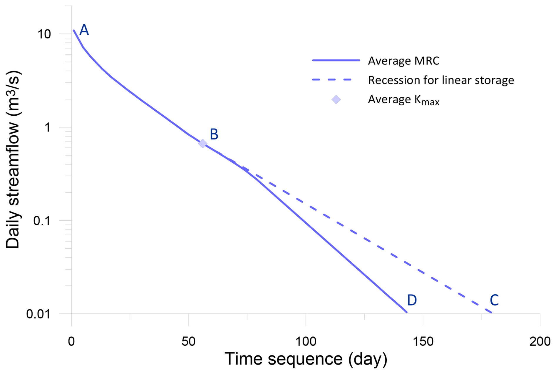
Figure 1 Example of an average Master Recession Curve (MRC) for Gibbo River at Gibbo Park (401207) including baseflow for a linear model and the average maximum recession coefficient (K_max). ABC is an average MRC plot whereas ABD is an average MRC incorporating the effect of transmission loss.

2.1 Development of Master Recession Curve

An MRC is commonly shown as a plot of daily streamflow (logarithmic scale) as a function of time as in Fig. 1. From A to B, the MRC is upwardly concave until the flow reaches the maximum recession constant (B) (location of minimum recession slope) after which the logarithm of flow decreases linearly (B to C). If there is transmission loss (stream evaporation or evapotranspiration from the adjacent riparian zone or leakage to the stream bed) the MRC follows B to D. The difference in the curves (B–D) and (B–C) is transmission loss, as defined by Boughton (2015).

An MRC represents the average rate of decline in streamflow following rainfall after surface runoff contributions have ceased. The average rate of decline is determined from the analysis of many individual recessions. The recession shape at any point in time depends on the initial water content of the unconfined aquifer and other sub-surface processes that together feed the stream. Also, as noted above, transmission losses affect recession shape. The initial water content of the aquifer/s and sub-storage systems is a result of the preceding climate and weather conditions and aquifer antecedent storage, as observed by Bart and Hope (2014). In our analysis we recognise that while the MRC is normally considered to represent the average rate of decline, it is sensible to characterise the natural variability (or aleatory uncertainty) in the MRC that arises from variable antecedent hydroclimatic conditions and heterogeneous storage conditions in the aquifer. Hence, in contrast to others (Tallaksen, 1995; Duncan, 2019), we hypothesise that there is a continuum of recession curves that can be represented either by a single MRC representative of average conditions, or else by a continuum of curves that result from variability in the initial water content of the aquifers feeding the stream and from the spatial heterogeneity in their physical configuration. These storages range from being full following a very wet period to a near empty condition following a long dry period. In our analysis, these two extreme conditions are notionally represented by MRCs for 90th percentile and 10th percentile exceedance frequency curves respectively. Three intermediate conditions are also included: 75th percentile represents recessions following a moderate wet period, whereas 25th percentile is for conditions following a moderate dry period. The “typical” initial condition is represented by a 50th percentile MRC. Here, we express variability in terms of an exceedance probability rather than in terms of a physical variable, for example, antecedent rainfall. That is, in a given catchment in a moderately dry condition, it might be reasonable to expect that an individual recession might follow an MRC that is exceeded 25 % of the time, and another individual recession following wetter conditions might follow an MRC that is exceeded 75 % of the time. We adopted this approach in McMahon and Nathan (2025). It is not inconsistent with Fiorotto and Caroni (2013), who analysed the structure of the recession curve within a stochastic rather than in a deterministic framework.

An important parameter associated with an MRC is the maximum recession constant (K_max). As observed in Fig. 1, it is the point where the recession curve reaches minimum slope and without transmission losses would continue recessing at that slope. It has been used by many researchers under different guises. For example, it is related to the characteristic time (Brutsaert and Lopez, 1998), and used to estimate residence time (Chapman, 2003). Boughton (2015) utilised the maximum recession constant in estimating transmission losses in streams and McMahon and Nathan (2025) adopted K_max as a key to their procedure to estimate hydraulic properties of unconfined aquifers from daily streamflow data. In Sect. 4, we adopt K_max to represent the slopes of the continuum of MRCs as they move from wet to dry antecedent conditions.

It is rare for observed daily streamflows to be available for long periods without being impacted by rainfall or observational tolerance issues, or by measurement malfunction, and so plots of actual recessions (streamflow volume Q vs. time t) rarely show a complete shape of the recession. Virtually all investigators are confronted with these problems.

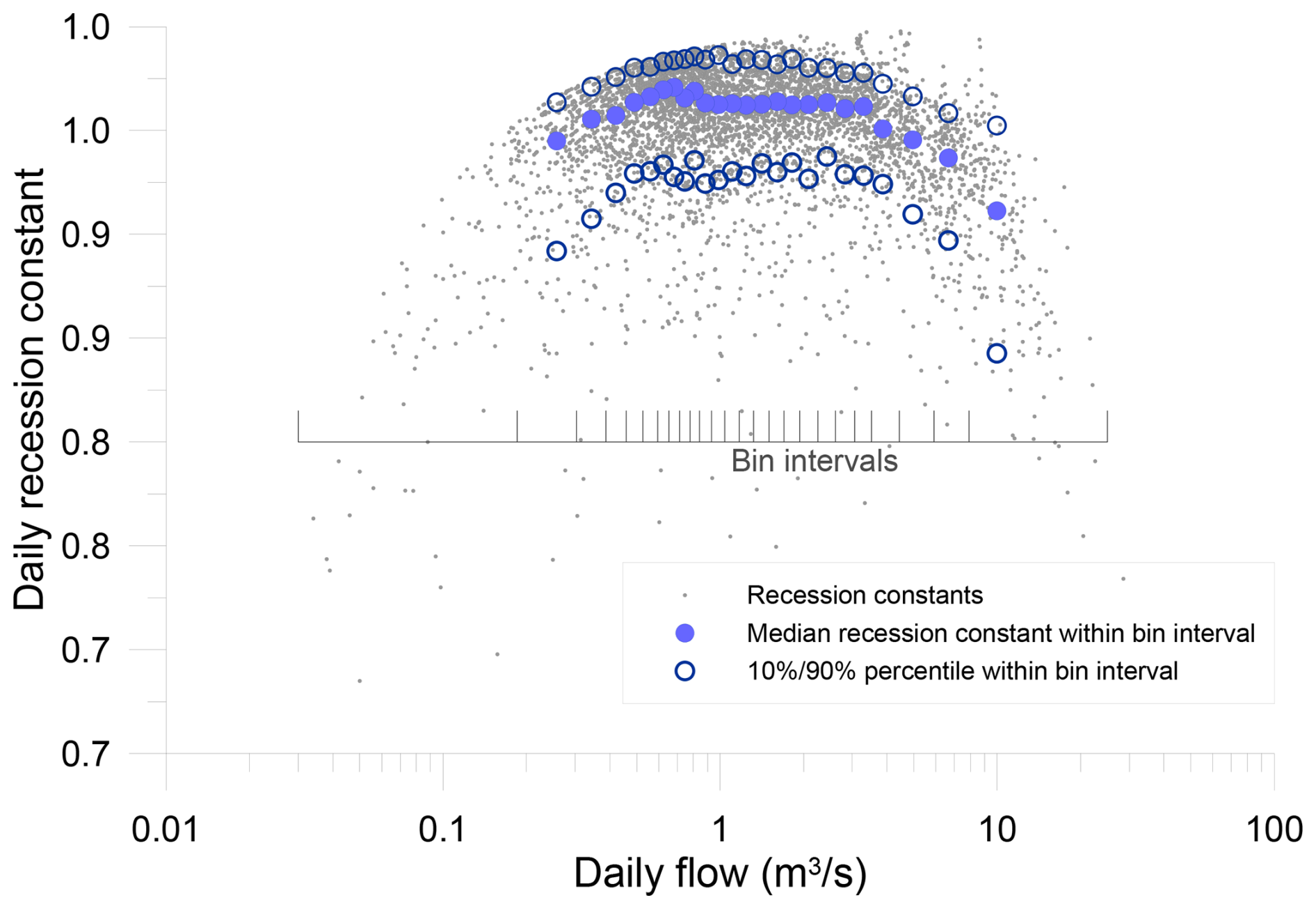
Figure 2 Relationship between daily recession constant and daily flow for Gibbo River at Gibbo Park 110 (401217) showing median, 10th percentile, and 90th percentile recession constants in each bin of 200 values.

The exceedance percentile values for the MRC are estimated from binned values of daily K_j (recession constant) and Q_j pairs following the correlation method (Hall, 1968; Beran and Gustard, 1977; Boughton, 2015) which is adopted herein to compute an MRC. The key steps in the correlation approach are:

1. Daily recession constants (K_j) (where $K_j=Q_j/Q_{j-\mathrm{1}}$, for $\mathrm{0}<K_j<\mathrm{1}$), and Q_j (daily discharge at time j) are ranked as pairs (by Q_j) after values potentially affected by rainfall are discarded. The number of rain-impacted days to be discarded is a function of catchment area guided by Linsley et al. (1982, Eq. 7-4). We have not included adjustment for data imprecision (Rupp et al., 2009) because we compare the computed MRC with observed recession data.

2. The ranked pairs are binned using a constant bin size of around 200 items (Fig. 2). This arbitrary decision permits the statistics (mean, median and percentiles from 10 % to 90 %) of the K_j and Q_j values to be estimated with confidence. 200 is adopted so long as there are sufficient bins to determine which bins hold the maximum value of each statistic. Again, this is a subjective decision in which we adopt a minimum of five bins.

3. For each bin and based on K_j, a range of exceedance percentiles (10 % percentile, 25th percentile, 50th percentile, 75th percentile and 90th percentile) are computed. Figure 2 is an example of the bins showing K_j and Q_j values. To provide for varying initial conditions according to catchment wetness (and hence the initial averaged state of the unconfined aquifer storage), the 10th percentile, 25th percentile, …, and 90th percentile daily Q values are also estimated. Thus, the initial 10th percentile discharge is associated with the 10th percentile MRC, and so on.

4. The final step is to construct the MRCs. For a given percentile (say 90th percentile), the MRC is estimated as described by Boughton (2015, p. 45). Begin at the highest value of daily flow in the record of K_j plausible values defined by point 1 above. The next highest value Q in the MRC is calculated by multiplying the highest value by the 90th percentile rate of recession in the daily flow range of the highest flow. The next value is calculated by multiplying that value by the 90th percentile rate of recession in the daily flow range of the result. This is continued until the flow rate becomes smaller than the lowest flow rate in the record. This process is carried out for each percentile. An example of an MRC computed in this manner is presented as Fig. 3.

5. The maximum recession constant for a given percentile is obtained from the binned values (Fig. 2); example values are plotted in Fig. 3.

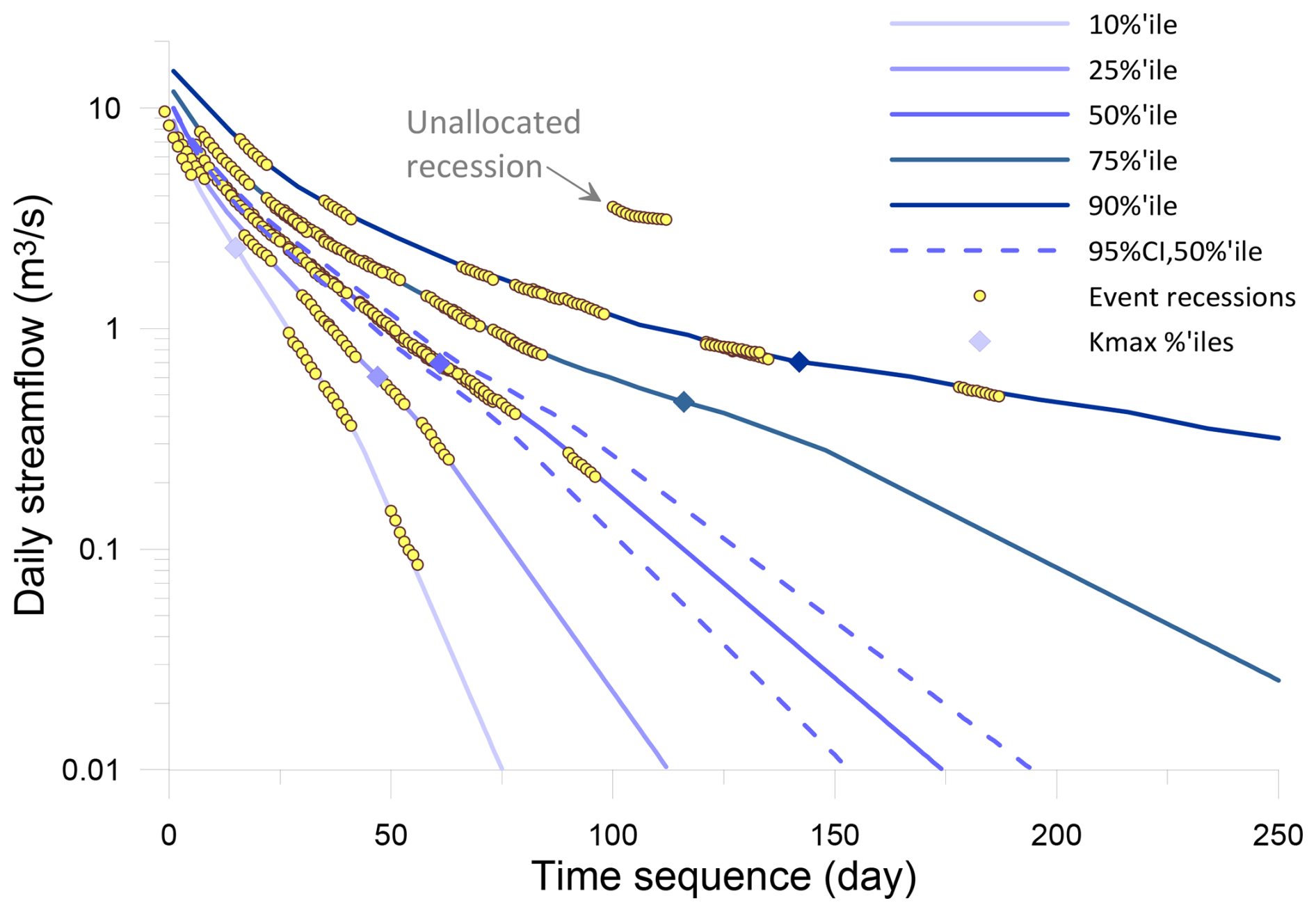
Figure 3 Comparison of daily MRCs computed using a constant bin correlation method with observed recessions during rainless periods for Gibbo River at Gibbo Park (401217). Three rainless days were required before data were acceptable in the analysis. The computed recessions are for five percentile values: 10 %, 25 %, 50 %, 75 % and 90 %. Maximum recession constants are located in the figure. The 2.5 % and 95.5 % confidence limits (CL) for the 50 % MRC estimated using bootstrapping are also included. One acceptable recession was not allocated to one of the five MRCs.

2.2 Selection and superposition of recessions

In accepting the daily observed recessions for plotting (as in Fig. 3), we adopted the following guidelines:

1. Choose at least ten consecutive decreasing daily discharges that are for days unimpacted by rainfall. The first x d are not used in plotting the observed recession to reduce the potential for surface runoff to affect the recession. Here, “x” d is defined by Linsley et al. (1982, Eq. 7-4).

2. Acceptable recessions superimposed on the MRC (log Q (ordinate) versus time (abscissa) graph) should be gently concave (representing non-linearity), convex (after the maximum recession constant, i.e. affected by transmission loss), or a straight line from the maximum recession constant, i.e. the discharge is from a linear storage system not exhibiting transmission loss. This latter condition is most unlikely as all streams will have evaporation/evapotranspiration loss, although in some cases the loss may be too small to affect the daily discharge estimates.

3. Discharges that diverge upward from the main curve are deleted. These could occur at either end of the plotted observed daily time-series. The earlier values may be the result of some residual surface runoff not being removed by waiting x d before the plot begins. Or the last value (or last few values) could be the result of catchment rainfall (and, therefore, runoff) not identified in the observed rainfall data.

4. The resulting plotted data should have at least seven consecutive recessive data points, i.e. the recession does not include days with equal discharge. This 7 d limit is subjective and there is a trade-off between sufficient data points to define a recession and sufficient recessions to define portions of the master recession curve. Others have used 12 d (Hameed et al., 2023), 10 d (van Dijk, 2010), 7 d (Whitaker et al., 2022), 6 d (Gao et al., 2023) and 5 d (Parra et al., 2023).

Table 1 Attributes of study catchments and details of plotted recessions.

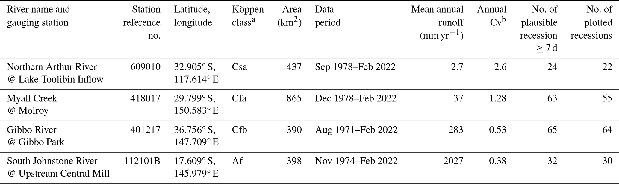
^a Csa: temperate, dry hot summer; Cfa: temperate, no dry season, hot summer; Cfb temperate, no dry season, warm summer; Af: tropical, rainforest (Peel et al., 2007). ^b Cv: coefficient of variation of annual streamflows.

2.3 Study catchments

The comparison between the computed MRCs and observed recessions was made for four streams as set out in Table 1. They span a wide range of hydrology across Australia as defined by mean annual catchment runoff from about 3 to 2000 mm yr⁻¹.

As noted above, the number of raindays to be eliminated prior to plotting the recessions is a function of catchment area; for Gibbo, Northern Arthur and South Johnstone Rivers 3 d were eliminated, whereas for Myall River the initial 4 d of recessions were eliminated.

3 Application

For each stream, MRCs were computed (as set out in Sect. 2.1) for five exceedance percentiles: 10 %, 25 %, 50 %, 75 % and 90 % values, representing very dry initial conditions (10th percentile) to very wet initial conditions (90th percentile). The resulting MRCs obtained for Gibbo River at Gibbo Park are shown in Fig. 3.

For illustration purposes here it is useful to demonstrate how observed recessions resulting from different antecedent conditions may be superimposed on the different percentile MRCs (Fig. 3). This was done manually by moving the plotted observed recession parallel to the time axis until the observed recession matched one of the five selected percentile values. Also plotted on Fig. 3 are the maximum recession constants for each condition (as set out in Sect. 2.1). Equivalent plots for other sites are in the Supplement. There is some subjectivity involved in this process, but this is of little concern as the purpose here is merely to illustrate how different recessions can be mapped to different sets of antecedent conditions. That is, rather than treat deviations of observed recessions from the MRC as a source of unexplained uncertainty (e.g. Nathan and McMahon, 1990; Singh and Griffiths, 2021), the degree to which an observed recession conforms to a specific percentile MRC provides an indication of the exceedance probability of the governing antecedent conditions. For example, the “unallocated” recession shown in Fig. 3 has not been mapped to one of the five derived MRC percentiles, but it lies on, or above, the 90th percentile MRC; accordingly, it may be inferred that the recession occurred at a time when catchment storage levels were at the wettest 10 % of historic conditions. Of course, if we had computed MRCs for ten exceedance percentile values rather than just for five (i.e. for 10 %, 20 %, … 90 % rather than 10 %, 25 %, 50 %, 75 %, 90 %), then some of the observed recessions shown in Fig. 3 would have matched the computed MRCs more closely. Certainly, if we had chosen only three MRCs, then many of the observed recessions would not fit the computed MRCs. We are satisfied that the adoption of five MRCs covering a range of conditions is sufficient and satisfactory to show that catchment recessions can be represented by a continuum of MRCs rather than a single average MRC as has traditionally been adopted.

The number of plausible observed recessions plotted in the figures (Fig. 3, and in the Supplement) is listed in the last two columns of Table 1. The numbers varied from 24 for Northern Arthur to 65 for Gibbo whereas the final numbers plotted and notionally allocated to one of the five representative percentile MRC curve varied from 22 for Northern Arthur to 64 for Gibbo. It is seen that the vast majority of recessions can be mapped reasonably well to the limited number of percentile curves provided, which serves to illustrate the concept that any differences in slope between an individual recession and an average MRC can be explained by differences in antecedent conditions, as represented by the MRCs of different percentiles.

To further illustrate the robustness of manual allocation of the observed daily recessions, for each recession in the Northern Arthur data (Fig. S3, Supplement) the magnitudes of the observed daily recession discharges were compared to the modelled recession discharges. Two metrics were computed based on the observed and modelled recessions: the standard correlation coefficient and the Nash-Sutcliffe Efficiency (Nash and Sutcliffe, 1970). The median correlation coefficient was 0.995 and the median Nash-Sutcliffe efficiency was 0.962, where the differences between the minimum and maximum of these statistics were 0.015 and 0.315, respectively. Overall, the values for both metrics are high, confirming the adequacy of the manual allocation to the selected percentile MRCs.

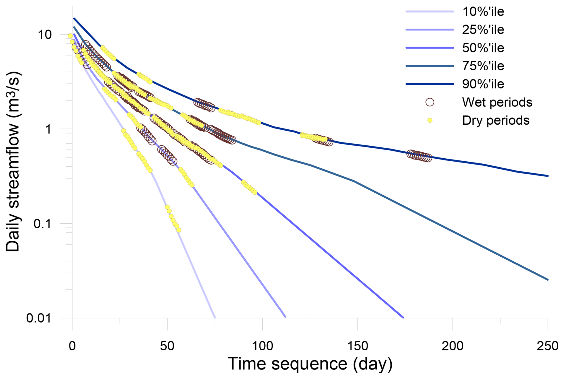
Figure 4 Comparison of observed daily recessions for data drawn separately from the wet 6-months and dry 6-months periods superimposed on the estimated MRCs for Gibbo River at Gibbo Park (401217).

Figure 4 considers the influence of wet and dry periods on the plotted data for Gibbo River. The plots were compiled for the wet and the dry 6-months periods. The two periods were based on the mean monthly streamflows for Gibbo River at Gibbo Park in which the average streamflow during the wet period from July to December was 3.9 times the average streamflow during the dry period, January to June. It is noted for these seasonal conditions that recessions were identified for the five dry periods, but no observed recessions representing wet conditions were available for the 10th percentile curve.

4 Discussion

4.1 Representation of natural variability

The observed recessions for all four streams (shown in Figs. 3 and 4, and in the Supplement, a total of 169 across the four streams) plot neatly on the computed MRCs. This is expected, of course, as both sets of results are drawn from the same data. Furthermore, the range of behaviour between the 10th percentile to 90th percentile MRCs provides much scope to ensure the observed recessions fit reasonably well to one of the five curves. The plots for Myall River (Fig. S2) are an exception where eight recessions were not allocated to one of the five MRCs. Most would have plotted on intermediate MRCs.

We have not found plots similar to Fig. 3 in the literature comparing observed recessions with probabilistic curves, although Kienzle (2006) identified two very different MRCs for a 7675 km² watershed in Alberta, Canada. Fiorotto and Caroni (2013, Fig. 6) incorporated a range of recessions as a function of probability by interpreting the master recession in terms of a stochastic process. On the other hand, Yang et al. (2019) developed separate MRCs for four flow regime conditions, high, moist, low, and dry and, separately, for the four climate seasons. The approach by Gao et al. (2023), inter alia, is similar to our method but they do not map the observed data to the developed recessions.

Our plots confirm that the adopted correlation method to estimating MRCs is a valid alternative to other approaches and is easily adapted to characterising natural variability and uncertainty. An important feature of Fig. 3 is that the observed recessions extended beyond the day of their respective maximum recession constants, even for the extremely wet South Johnstone catchment with a mean annual runoff of more than 2000 mm yr⁻¹ (Fig. S1) where there is evidence of transmission loss. Some studies (for example, Millares et al., 2009) involving recession analysis (Q∼t) that produce Q∼t diagrams do not extend the time scale much beyond the maximum recession constant, presumably in the belief that the curve continues in a concave manner. We highlight this point as few journal papers dealing with Q∼t recession analysis address this important feature of an MRC.

Another point to note relates to the confidence with which we can estimate the different percentile MRC curves. As pointed out earlier, we are suggesting the different percentile MRC curves represent the natural variability in the initial level of stored water in the different aquifer units feeding the stream; in other words, the source of variability is the aleatory uncertainty due to antecedent conditions and its influence on a catchment with spatially heterogeneous physical properties.

However, our ability to identify the different percentile MRCs is limited by the period of available observations, where the uncertainty around the derived MRCs increases as the sample size decreases. This source of uncertainty represents the epistemic uncertainty due to sampling variability and can be characterised by non-parametric bootstrapping. To this end, the uncertainty around a given percentile MRC is characterised by resampling (with replacement) estimates of the recession constant within each bin. An example of the epistemic uncertainty around the median MRC for Gibbo River is shown by the (dashed) confidence lines in Fig. 3. For the available data, it is seen that the epistemic uncertainty is much smaller than the aleatory uncertainty.

The characterisation of aleatory uncertainty as discussed herein can be applied to any application of an MRC analysis. One example of this is the estimation of the frequency of occurrence of transmission losses in streams, where the losses are based on MRCs (Boughton, 2015). Another example is the estimation of storage residence times in unconfined aquifers derived using the maximum recession constant, which is a key component of an MRC (McMahon and Nathan, 2025).

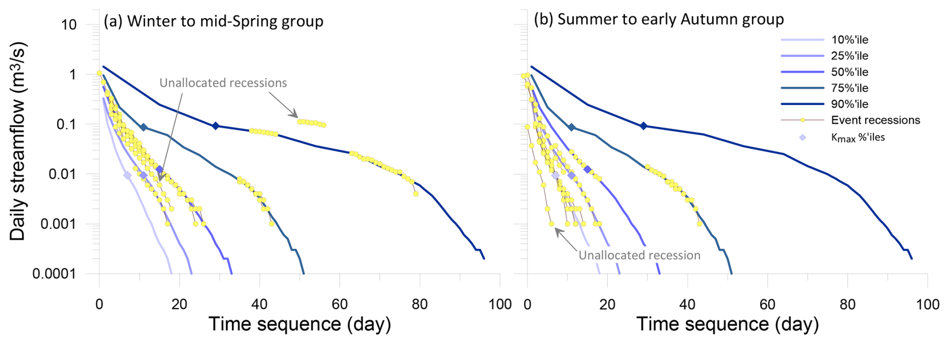
Figure 5 Comparison of computed daily MRCs for Northern Arthur River at Lake Toolibin Inflow (609010) with observed recessions during rainless periods for (a) winter to mid-spring and (b) summer to early autumn seasons. In both plots, the computed recessions are the same, based on all available data. Three rainless days were required before data were acceptable in the analysis. The recessions are for five percentile values: 10 %, 25 %, 50 %, 75 % and 90 %. Maximum recession constants are shown in the figure. Three acceptable recessions were not allocated to one of the five MRCs.

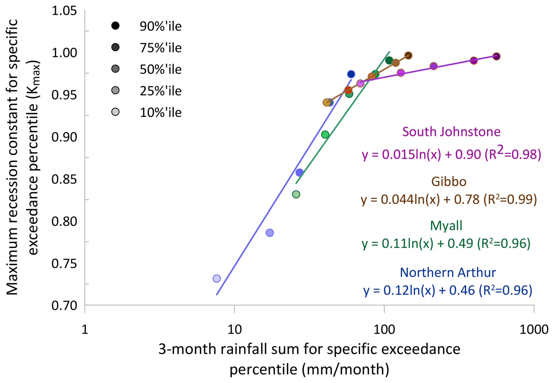
Figure 6 Maximum recession constant plotted against 3 monthly rainfall sums for specific exceedance percentiles: 10 %, 25 %, 50 %, 75 % and 90 % (as indicated by degree of shading shown in plot legend). Results are provided for four catchments: Northern Arthur, Myall, Gibbo and South Johnstone.

4.2 Seasonality

Analysis of recessions separately for the wet and dry 6-month periods for Gibbo River (Fig. 4) shows that the observed dry period recessions extend across the five computed MRCs whereas the observable recessions for the wet period cover mainly the 25th, 50th, 75th and 90th percentile MRCs. This distribution across the two periods is observed even though the dry 6-month period yields about one quarter the runoff generated during the wet period. The figure is important in that it demonstrates the difficulty in classifying catchment conditions in terms of general wet and dry periods, probably because we are examining the behaviour of individual events.

Two plots are provided for Northern Arthur. Figure 5a shows the recession data for the winter to mid-spring period whereas Fig. 5b is for the summer to early autumn period. The recession variability between summer and winter, which is characteristic of catchments in south-west Western Australia with perched water tables, is discussed in detail by George and Conacher (1993). Noting that at the Lake Toolibin stream gauging station for Northern Arthur River, there are, on average, only 43 d of flow per year and so the number of plausible recessions is limited. It is also noted that the minimum flow plotted in these figures is about five times larger than the minimum that can be measured under field conditions (McMahon and Peel, 2019). It is comforting to note that for this stream the observed recessions in Fig. 5 are, overall, consistent with the computed MRCs. The episodic nature of the Northern Arthur River hydrology is evident in Fig. 5 where the two of the three unallocated recessions are for climate conditions more extreme than the 10 % to 90th percentile plotted range.

Another way to explore seasonality is to relate the continuum of MRCs to a measure of antecedent climate; a simple measure is antecedent rainfall. The results of such an analysis are shown in Figs. 6 and S4a, b, c and d where the maximum recession constant (K_max) is plotted against antecedent (monthly) rainfalls for specific exceedance percentiles. Here antecedent rainfalls for stations within or near the catchment are defined as the 10 % percentile exceedance of one month, 3-month sums, 5-month sums, 7-month sums and 11-month sums for very dry antecedent conditions, and the same range of antecedent rainfalls for 25 % (dry), 50 % (“average”), 75 % (wet) and 90 % (very wet). The rainfalls are for independent sums rather than overlapping sums. It is observed in Fig. 3 that K_max (the minimum slope of a given recession) is an appropriate metric to represent the continuum of MRCs because as K_max increases in slope the MRCs move from wet to dry antecedent conditions as illustrated in Figs. 3 and S1, S2 and S3. In Fig. 6, K_max is strongly related to 3-month sums of rainfall. It is equally correlated with 1 month, 5 months, 7 months and 11 months sums (see Fig. S4a, b, c and d). Because of the high correlations among the 1 month, 3 months, 5 months, 7 months and 11 months sums (Table S1 in the Supplement), we cannot say without further analysis which duration is the most appropriate for a specific catchment. Such an analysis is beyond the scope of this study. What is evident, however, is that the continuum of MRCs is strongly correlated to antecedent rainfalls thus confirming our hypothesis that MRCs are the result of varying antecedent climate and weather conditions and are represented by a continuum of MRCs rather than a single average MRC.

4.3 Hypothesis based on inductive reasoning

But what is the explanation for the variability exhibited in Figs. 3 to 5? Our proposed hypothesis is that, in the catchments we are considering, there are many sub-catchments (they have Strahler stream orders greater than three; Strahler, 1957) with unconfined aquifers and delayed sub-surface flows. These sub-surface storages vary greatly in terms of dimensions, hydraulic properties, location and elevation relative to the nearest stream channel. This heterogeneity within a catchment combined with a varying weather and climate is hypothesized to produce a continuum of MRCs as illustrated in the Figs. 3 to 5.

Because Northern Arthur is, hydrologically speaking, a well-instrumented and researched catchment (Callow et al., 2007, 2020), it is used to assess a qualitative model explaining the observed variability (aleatory uncertainty) in the MRCs (Fig. 5; see also Plates S1 and S2 in the Supplement which show, respectively, the mid-western catchment and the stream gauging station location). Consider Fig. 5a and b which show the recessions for Northern Arthur River. Two periods of activity are identified; the number of recessions over the winter to mid-spring period are twice that over summer to early autumn (Fig. S5). We deduce that the very steep 10th percentile MRC that occurs over about 15 d following rain on a very dry catchment occurs from an unconfined aquifer (denoted as “A”) with very high hydraulic conductivity. On the other hand, the considerably flatter 90th percentile MRC occurs after a very wet period and is likely fed from an aquifer (denoted as “B”) that exhibits a much more attenuated response to rainfall due to having either larger storage or lower hydraulic conductivity. For simplicity, we assume that these two aquifers, A and B, are in parallel and are the only groundwater sources discharging to the stream. After a very wet period that fills both aquifers, aquifer A will empty very quickly while aquifer B will dominate the recession. However, if aquifer A, the less attenuated aquifer, is located in the catchment such that after a long dry period there is sufficient rain to replenish it yet insufficient for aquifer B to discharge, a steep recession will result. This explanation must be tempered by noting that stream evaporation transmission losses probably will be high during the summer to early autumn periods (average area potential evapotranspiration (AAPE) ∼5 mm d⁻¹) but much less during the winter to mid-spring periods (AAPE ∼2.5 mm d⁻¹) (Wang et al., 2001). Adopting two parallel storages for aquifer modelling is not unusual (see for example, Moore, 1997, and Gao et al., 2017, although they assumed linear systems).

The above simple qualitative two-stage model of the surface water-groundwater connectivity proposed for the Northern Arthur catchment is not inconsistent with the three-stage surface water-groundwater connectivity and vertical recharge processes described by Callow et al. (2020). Their description is based on intensive instrumentation of the catchment and detailed analyses. As described by Callow et al. (2020), during the winter period soils saturate and macropores close, matrix flow dominates, and surficial aquifers become connected; although a vertical hydraulic gradient continues, the system acts as a semi-confined aquifer, and as the aquifers connect, a transition to the bottom-up groundwater discharge occurs. This description applies to the winter to mid-spring period resulting in the observed recessions depicted in Fig. 5a. From late spring, groundwater levels fall and, as the system dries, de-coupling between the surface and groundwater occurs, and macropores re-develop. Valley floor areas dry with large surface cracks. Top-down recharge occurs as a result of high infiltration facilitated by the macropores and surface flows. Observed recessions in Fig. 5b are the result of these processes. In their discussion of the surface-subsurface processes involved, Callow et al. (2020) describe the transitions between the two main stages of low flow generation in Northern Arthur catchment. Referring to Fig. 5, we surmise that some of the intermediate recessions (75 %, 50 % and 25th percentiles) represent these transitions as the system passes from a wet period to a dry period and back again to the next wet phase.

5 Conclusions

This comparison between computed master recession curves (MRCs) and observed recessions for rainless periods confirms the usefulness of the computed MRC constructed using correlation between adjacent days. Our analyses confirm our hypothesise that there is a continuum of recession curves that can be represented by a single average MRC or by a family of percentile MRCs in which the variability across the continuum is the result of variable antecedent conditions in the unconfined aquifers and other sub-surface storages, their relative location, and the heterogeneity of their hydraulic properties. Our proposed approach is consistent with field data from the Northern Arthur catchment. The master recession curves examined herein support the notion that MRCs should be examined beyond the maximum recession constant to provide a more complete picture of the MRC than is often portrayed in the published literature.