How well do hydrological models simulate streamflow extremes and drought-to-flood transitions?

Flood impacts can be enhanced when they occur shortly after droughts. Hydrological models are useful tools to better understand the underlying processes and mechanisms driving the response of floods occurring in close succession to streamflow drought. However, it is yet unclear how well hydrological models capture these compound extreme events and which modeling decisions are most important for model performance. To address this research gap, we calibrated four conceptual bucket-style hydrological models with different structures (GR4J, GR5J, GR6J, and TUW) for 63 catchments located in Chile and Switzerland using different calibration strategies. Specifically, we assessed the relative importance of different methodological choices in simulating and detecting observed drought-to-flood transitions, including model structure, streamflow transformation, and the Kling–Gupta efficiency (KGE) formulation and weights used to calibrate the model parameters. We demonstrate that model performance, as expressed by the KGE, does not guarantee a good performance in terms of detecting streamflow extremes and their transitions. Further, we show that a model's performance with respect to capturing extreme events primarily depends on how well it captures streamflow timing. Our results also highlight that model structure, catchment characteristics and meteorological forcings play a key role in the detection of transitions. Overall, we find that model representation of drought-to-flood transitions is generally poor, especially in semi-arid and high-mountain catchments compared to humid low-elevation catchments. Ultimately, our study provides insights for further model improvements to simulate and better understand drought-to-flood transitions and to identify regions prone to this hazard.

1 Introduction

Hydrological extreme events such as streamflow droughts and floods are expected to become more frequent, severe, and persistent in a warming climate (e.g., Gu et al., 2023; Asadieh and Krakauer, 2017; Martin, 2018; Tabari et al., 2021). This can lead to severe impacts on infrastructure, agriculture, water supply, and hydropower generation (e.g., McClymont et al., 2020; McMartin et al., 2018; Lehner et al., 2006; Sivakumar, 2011; Wasti et al., 2022), as well as social and political systems (e.g., Doocy et al., 2013; Hurlbert and Gupta, 2017; Kiem and Austin, 2013; Visconti, 2022).

Studies focusing on hydrological extreme events and their impacts often assume temporal and/or spatial independence between them, neglecting that extremes may be multivariate phenomena (Banfi and De Michele, 2022; Brunner, 2023). However, the impacts of floods can be enhanced when they occur during or shortly after dry periods (e.g., Barendrecht et al., 2024; Swain et al., 2018; He and Sheffield, 2020; Rashid and Wahl, 2022). For instance, Handwerger et al. (2019) and Valenzuela et al. (2022) have demonstrated an increase in the occurrence of landslides in California and Chile due to shifts from meteorological drought to intense precipitation. Similarly, Dietze et al. (2022) have shown that the 2018–2020 drought in Europe enhanced debris mobilisation during the 2021 flood in the Eifel region of western Germany and Belgium. In 2017, intense precipitation broke the 2012–2016 drought in California and led to severe flooding, the activation of the emergency spillway of the Lake Oroville dam for the first time in its history, and the declaration of emergency (Griffin and Anchukaitis, 2014; Robeson, 2015; Wang et al., 2017). Despite evidence of the interactions between drought and flood events, they are still most frequently studied independently (e.g., Ward et al., 2020; Quesada-Montano et al., 2018; Di Baldassarre et al., 2017).

The transition from drought to flood can occur within hours or days, whereas the transition from floods to droughts can range from weeks to years, leading to different water management challenges and reaction times for decision-makers (Hammond et al., 2025). Due to the inherent asymmetry in spatiotemporal characteristics and underlying drivers, as has been recently reviewed by Swain et al. (2025) from both meteorological and hydrological perspectives, drought-to-flood transitions often have more severe impacts than flood-to-drought transitions.

Both hydrological droughts and floods are linked to meteorological conditions such as precipitation surplus/deficit or low/high evapotranspiration rates. However, it has been shown that meteorological dry-to-wet spells are only weakly associated with hydrological drought-to-flood transitions, with a propagation rate of just 10 % within a 30 d period, and that wet spells are less likely to lead to floods than dry spells are to cause droughts (Brunner et al., 2025). Consequently, the occurrence and drivers of these compound events are not yet fully understood (e.g., Matanó et al., 2022, 2024; Brunner, 2023; Götte and Brunner, 2024; Hammond et al., 2025; Brunner et al., 2025). Similarly, it is yet unclear how increasing hydrological volatility in a warming climate (Swain et al., 2025) will translate to changes in drought-to-flood transition behavior.

Process-based hydrological models can provide valuable insights into how streamflow and/or other hydrological fluxes and states react to variations in meteorological and climate inputs (Hrachowitz and Clark, 2017). In recent decades, several efforts have been made to improve the realism of hydrological models in terms of spatial variability (e.g., Dembélé et al., 2020), the simulation of low (e.g., Garcia et al., 2017) and high flows (e.g., Mizukami et al., 2019), or the representation of flood-triggering mechanisms and spatiotemporal coherence (e.g., Brunner et al., 2020, 2021), under current and changing climatic conditions (e.g., Fowler et al., 2018). However, modeling hydrological extreme events such as droughts and floods is still challenging (e.g., Mizukami et al., 2019; Bruno et al., 2024), especially when multiple variables are involved. Such cases include, for example, modeling the dependence between flood peaks and volumes (Brunner and Sikorska-Senoner, 2019), or modeling the spatial dependence of floods happening in different locations (Brunner et al., 2021). This complexity suggests that capturing consecutive drought-to-flood events might not be trivial either. As model evaluations targeted at compound extremes have not yet been performed, it is still unclear how well hydrological models can, in fact, capture drought-to-flood transitions.

Hydrological modeling involves making decisions about model structure (i.e., process representations and parameterizations), spatial discretization, meteorological forcings, and parameter estimation approach (e.g., calibration/evaluation periods, hydrological target variables or signatures used in objective functions), which affect hydrological simulations and whose importance might vary depending on the modeling purpose (e.g., Mendoza et al., 2016; Mizukami et al., 2016; Baez-Villanueva et al., 2021; Guo et al., 2017; Melsen et al., 2019). Previous studies have highlighted that such modeling decisions can substantially influence simulated hydrological extremes and their uncertainties (e.g., Alexander et al., 2023; Melsen and Guse, 2019; Melsen et al., 2019). They have also shown that the choice of objective function for model calibration, model structure, and spatial discretization (forcings and domain) are the most influential decisions on modeling outcomes. While these previous studies have focused on analyzing the impacts of modeling decisions on drought and flood attributes (e.g., severity, duration), they have not looked at how these decisions influence event detection, i.e. whether or not a model can capture extreme events below or above a certain threshold. Moreover, previous work has focused on individual extremes instead of looking at them in a multivariate setting (Brunner, 2023). As such, it is unclear how individual modeling decisions might influence the representation of hydrological transitions.

Hydrological modeling often relies on a calibration process to find parameter values that minimize discrepancies between observations and simulations of a target variable (e.g., streamflow). The calibration process requires defining an objective function to measure the similarity between observations and simulations. In general, these objective functions are defined based on “least squares” formulations such as the widely used Nash-Sutcliffe Efficiency (NSE; Nash and Sutcliffe, 1970) and the Kling–Gupta Efficiency (KGE; Gupta et al., 2009). Although alternative objective functions have been proposed to enhance the robustness of calibrated parameters and hydrological consistency (e.g., Fowler et al., 2018; Yilmaz et al., 2008; McMillan, 2020), KGE and NSE remain widely used for model calibration and evaluation (e.g., Klemeš, 1986; Motavita et al., 2019; Seibert et al., 2019; Beven, 2025).

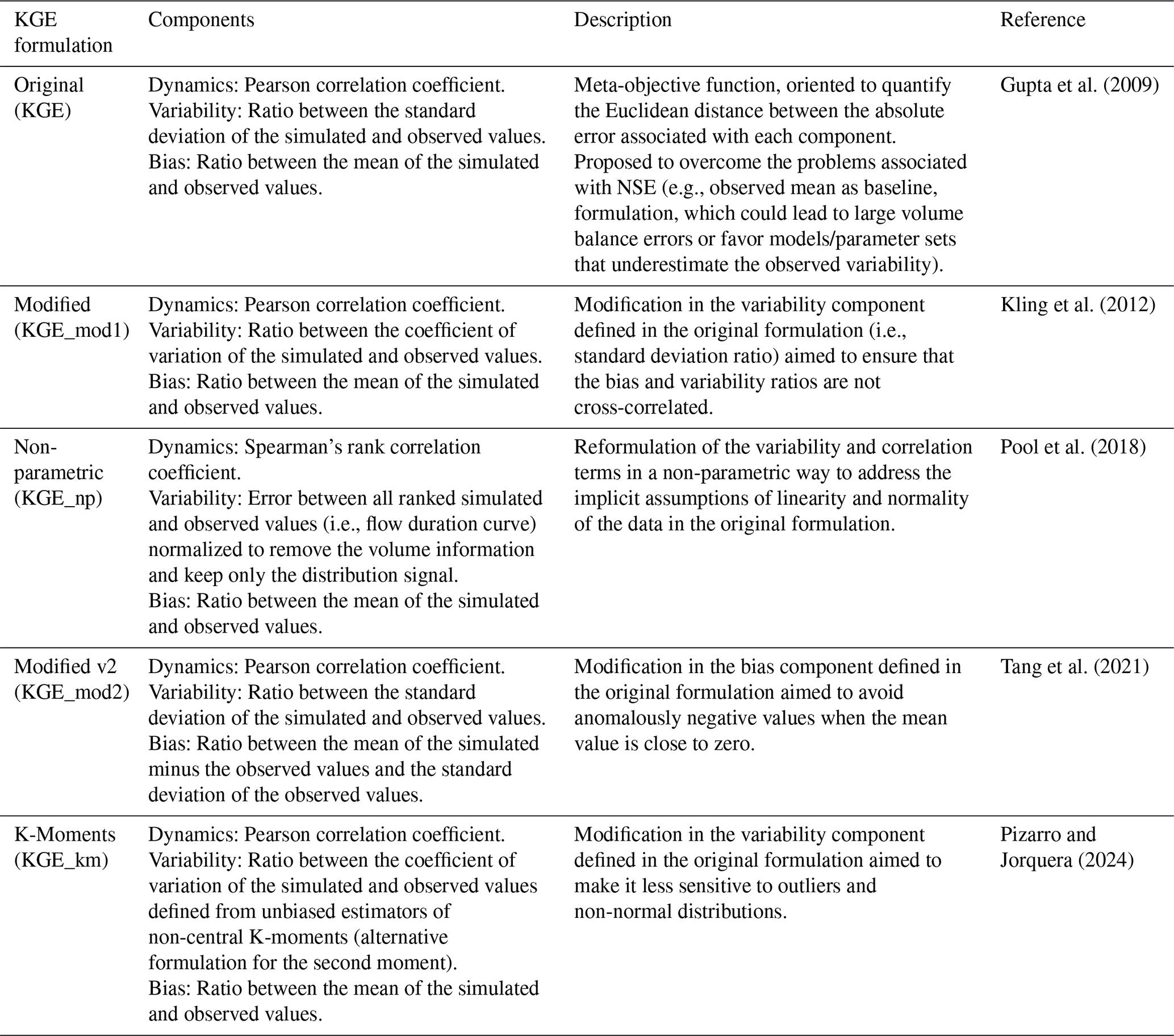
The Kling–Gupta Efficiency (KGE), originally proposed by Gupta et al. (2009), has been one of the most popular performance metrics used in hydrology over the last decades. Thanks to the possibility of disaggregating it into its three components – bias, variability, and correlation – KGE provides interpretability and diagnostic power. It has been applied for many modeling purposes, including the analysis of streamflow extremes (e.g., Gu et al., 2023; Hirpa et al., 2018). Calibrations are often considered successful if the KGE performance exceeds a certain threshold during both the calibration and evaluation periods (e.g., KGE > 0.4). It is also often assumed that the KGE criterion can be used as a proxy for how well a model represents streamflow properties such as extreme events (e.g., Lema et al., 2025; Cinkus et al., 2023; Zhao et al., 2025). However, model evaluations often do not explicitly evaluate how drought or flood events are represented at the event scale. As a consequence, it remains unclear how suitable of a proxy KGE and alternative formulations (Gupta et al., 2009; Kling et al., 2012; Pool et al., 2018; Tang et al., 2021; Pizarro and Jorquera, 2024) or adaptations (e.g., transformations and weights; Garcia et al., 2017; Wu et al., 2025; Mizukami et al., 2019) are for describing model accuracy in terms of extreme events and their consecutive occurrence.

In summary, it is unclear how different modeling decisions, such as the choice of the hydrological model, objective function, and streamflow transformations, affect drought-to-flood transition simulations and how well overall performance metrics, such as KGE, relate to a model's ability to capture streamflow extremes. It remains to be explored which modeling choices are most suitable for capturing these compound hydrological extreme events without compromising hydrological consistency (i.e., representation of different hydrological processes or properties). To address these research gaps, we investigate the extent to which hydrological models can represent consecutive drought-to-flood transitions and the impact of model structure and calibration choices on their representation. Specifically, we address the following research questions:

• How suitable is the KGE for calibrating models aimed at jointly simulating streamflow droughts and floods?

• Which modeling choices (e.g., model structure, KGE formulation, etc.) are most important for simulating droughts, floods, and their transitions?

• In which catchments are drought-to-flood transitions most challenging to model and detect?

To address these questions, we performed several calibration experiments with four conceptual bucket-type hydrological models (GR4J, GR5J, GR6J, and TUW) across 63 catchments in Chile and Switzerland. In our experiments, we tested different configurations of the Kling–Gupta efficiency (KGE) to assess their performance in simulating and detecting observed transitions. These configurations included five KGE formulations (Table 1), two streamflow transformations (i.e., Q and $\mathrm{1}/Q$) and their linear combination (i.e., $\mathrm{0.5}\times \text{KGE}\left(Q\right)+\mathrm{0.5}\times \text{KGE}(\mathrm{1}/Q)$), and four different weights applied to the variability term of the KGE ($c_{\mathrm{2}}=\mathrm{1},\mathrm{2},\mathrm{4},\mathrm{8}$). Secondly, we assessed the relative importance of each methodological choice for detecting events and ensuring hydrological consistency. Finally, we explored the link between model performance and hydrometeorological and physiographic catchment descriptors.

Gupta et al. (2009)Kling et al. (2012)Pool et al. (2018)Tang et al. (2021)Pizarro and Jorquera (2024)

Table 1 Summary of KGE formulations. In each formulation, the term dynamics stands for the representation of the temporal evolution of the target variable, while the terms variability and bias aim to characterize its distribution.

2 Study domain and data

The study domain encompasses 24 and 39 near-natural catchments in Chile (CL; Fig. 1a) and Switzerland (CH; Fig. 1b), respectively. These catchments are selected based on the availability of complete daily streamflow records between 1981 and 2020 for at least 30 years, with a complete year being defined as one in which all months had information for at least 90 % of the days. We characterize the hydroclimatology of the catchments in our study domain by the wetness index ($P/\text{PET}$), runoff coefficient ($Q/P$), p-seasonality and q-seasonality index, and fraction of precipitation falling as snow (fsnow) over the period 1985–2020. The p-seasonality index (Woods, 2009; Berghuijs et al., 2014), as well as its analogue, q-seasonality, describes the seasonality of precipitation (or streamflow) and the degree of synchronization with the temperature seasonality. The fsnow is computed according to the formulation proposed by Woods (2009) and ranges from 0 (all precipitation falls as rain) to 1 (all precipitation falls as snow).

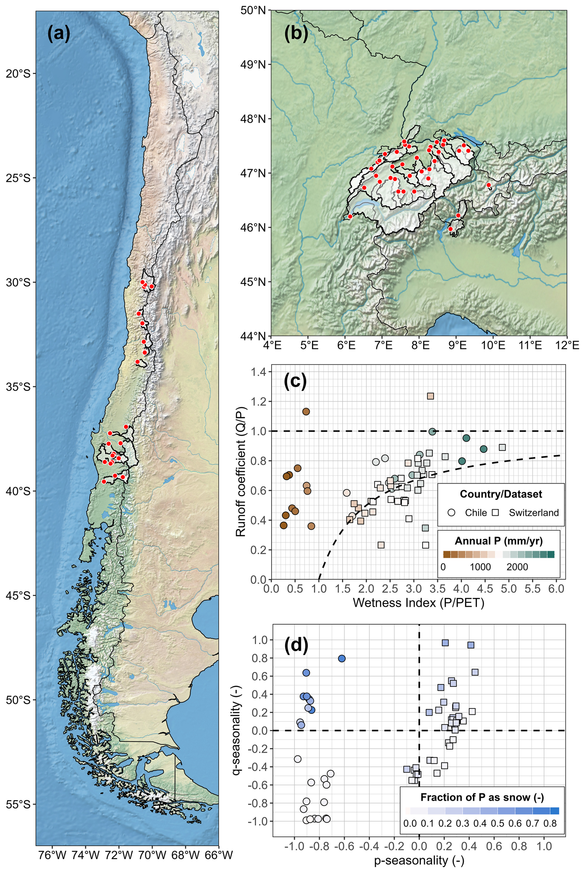
Figure 1 Study domain and hydroclimatic characteristics computed for the period 1985–2020 using data retrieved from CAMELS Chile (CL) and Switzerland (CH). Location of catchments across the study domain in (a) Chile and (b) Switzerland, (c) relationship between wetness index ($P/\text{PET}$), runoff coefficient ($Q/P$), and mean annual precipitation, and (d) relationship of seasonality of precipitation and streamflow and fraction of precipitation falling as snow. For p-seasonality and q-seasonality, positive (negative) values indicate summer (winter) dominated precipitation or streamflow, while values close to zero indicate a uniform distribution across the year.

This characterization shows that selected catchments span a wide range of hydroclimatic characteristics (Fig. 1c), from energy to water-limited, and different hydrological regimes (Fig. 1d), from snowmelt (e.g., p-seasonality < −0.5 and q-seasonality > 0.5) to rainfall-dominated (e.g., p-seasonality < −0.5 and q-seasonality < −0.5). Some catchments are positioned above the water limit (i.e., $Q/P=\mathrm{1}$) or below the energy limit (i.e., $Q/P=\mathrm{1}-\mathrm{1}/(P/\text{PET})$; Fig. 1c), which suggests an underestimation of precipitation – which might require correcting for precipitation undercatch (e.g., Newman et al., 2015; Stisen et al., 2012; Hughes et al., 2021) – or a surplus of streamflow due to, e.g., uncertainties in stage-discharge relationships or glacier and/or ground water contributions.

The CAMELS Chile (CL; Alvarez-Garreton et al., 2018a) and Switzerland (CH; Höge et al., 2023a) datasets are used to obtain the meteorological forcings, streamflow records, snow water equivalent (SWE) estimates, and catchment boundaries for the catchments in the two study domains. The meteorological forcings of both datasets, CR2Met version 2.5 for Chile (Boisier, 2023) and RhiresD version 2 for Switzerland (MeteoSwiss, 2021b, a), are based on local gridded observation-based products, while SWE products are based on a snow cover model and data assimilation (for more detail refer to Cortés and Margulis, 2017; Magnusson et al., 2014). We prefer these local products over global ones such as ERA5 (Hersbach et al., 2020) because of their reliance on observations and high horizontal resolutions (approximately 5 km × 5 km for CR2Met and 2 km × 2 km for RhiresD) that enable a better representation of precipitation patterns in the complex topography of our study domains. Further, these products have been widely used for hydrological studies in Chile (e.g., Vásquez et al., 2021; Alvarez-Garreton et al., 2021; Araya et al., 2023) and Switzerland (e.g., Peleg et al., 2020; Fatichi et al., 2015; Tuel et al., 2022). Streamflow records available through the CAMELS datasets were acquired from the national agencies in each country (i.e., the General Directorate of Water of Chile – DGA and the Swiss Federal Office for the Environment – FOEN). We compute topographic characteristics and hypsometric curves, which are needed to set up the snow routines, using the catchment outlines from CAMELS and the Multi-Error-Removed Improved-Terrain (MERIT) digital elevation model (Yamazaki et al., 2019). Additionally, we retrieve time series of actual evapotranspiration (ET) from the satellite- and reanalysis-based GLEAM v3.8a dataset (Miralles et al., 2011), which are spatially aggregated to the catchment scale and used to complement the model performance assessment.

3 Methodological approach

Our methodological approach is illustrated in Fig. 2. Four hydrological models were calibrated against observed streamflow records, using five different formulations of the Kling–Gupta efficiency (KGE) as objective functions. In addition, we tested three streamflow transformations and four different weights applied to the KGE variability term. This calibration experiment resulted in 60 optimal parameter sets per model and catchment (i.e., $\mathrm{5}\text{KGE}\times \mathrm{3}\text{transformations}\times \mathrm{4}\text{weights}$). We evaluated model performance based on (1) general goodness-of-fit metrics such as the NSE (Legates and McCabe, 1999; Althoff and Rodrigues, 2021), (2) simulation of extreme events and transitions between them using categorical indices, and (3) hydrological consistency in different processes related to streamflow, snow, and evapotranspiration by comparing simulated time series of these variables with observations or reference products. In this paper, we used the terms “formulation” to refer to a specific definition of the KGE (Table 1), “case” to refer to the application of KGE weights or flow transformations, and “configuration” to refer to the combination of a specific KGE formulation and a specific case using certain weights and a specific streamflow transformation. The cases without weights and/or the linear combination between streamflow without (i.e., Q) and with low-flow transformations (i.e., $\mathrm{1}/Q$) were used as a reference for the comparison of the results. To assess the statistical significance of the differences between, e.g., the ability to capture streamflow extreme events across models, as well as other configurations tested in this study, we applied the Wilcoxon test (Wilcoxon, 1945) at a 5 % significance level and provided p-values where possible. The Wilcoxon test is a nonparametric test used to determine whether two groups differ statistically, without making any specific assumptions about their distributions (e.g., normality). The following sections provide a detailed description of the different methodological steps.

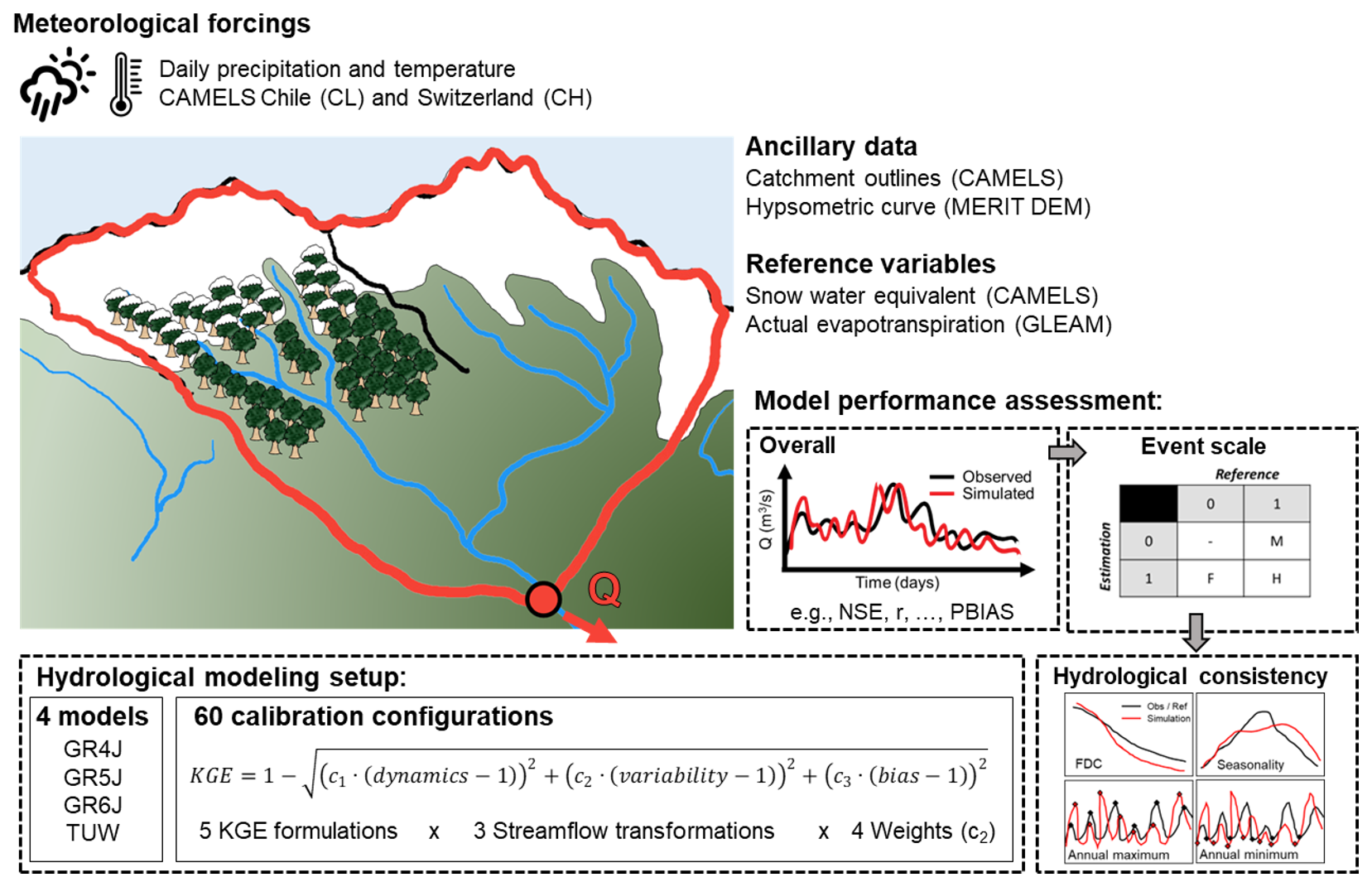
Figure 2 Overview of the methodological approach. See text for details.

3.1 Streamflow extremes characterization

We detected droughts, floods, and drought-to-flood transitions using the methods proposed by Götte and Brunner (2024). Their approach identifies periods of negative streamflow anomalies (i.e., droughts) using a daily varying threshold based on a 30 d rolling quantile of the daily streamflow data and high streamflow events (i.e., floods) using a fixed threshold based on a quantile of the annual maximum streamflow values. We further required that all drought events have a minimum duration of 30 d, and we merge droughts separated by fewer than 15 d (Van Loon and Van Lanen, 2012; Fleig et al., 2006; Tallaksen et al., 1997) to limit the detection of minor events. The thresholds for droughts (30th percentile of the smoothed daily flow) and floods (40th percentile of the annual maxima series) were set to ensure roughly one streamflow extreme event of each type (i.e., drought and flood) per year on average for each catchment (see Fig. S7 in the Supplement). This target was set in order to identify a statistically representative number of extreme events, comparable to the sample size that would be obtained by the commonly used annual maximum approach (e.g., Meylan et al., 2012). Using the flood and drought events identified, we, in a second step, identified transition events. Rapid (within 14 d) and seasonal (within 90 d) transitions are defined based on the number of days between the end of the drought and the onset of the flood, following Götte and Brunner (2024). Considering this definition and the thresholds adopted, we identified one transition event every 4 years on average for each catchment. Figure 3 illustrates the detection of droughts, floods, and their transitions for two catchments within the study domain.

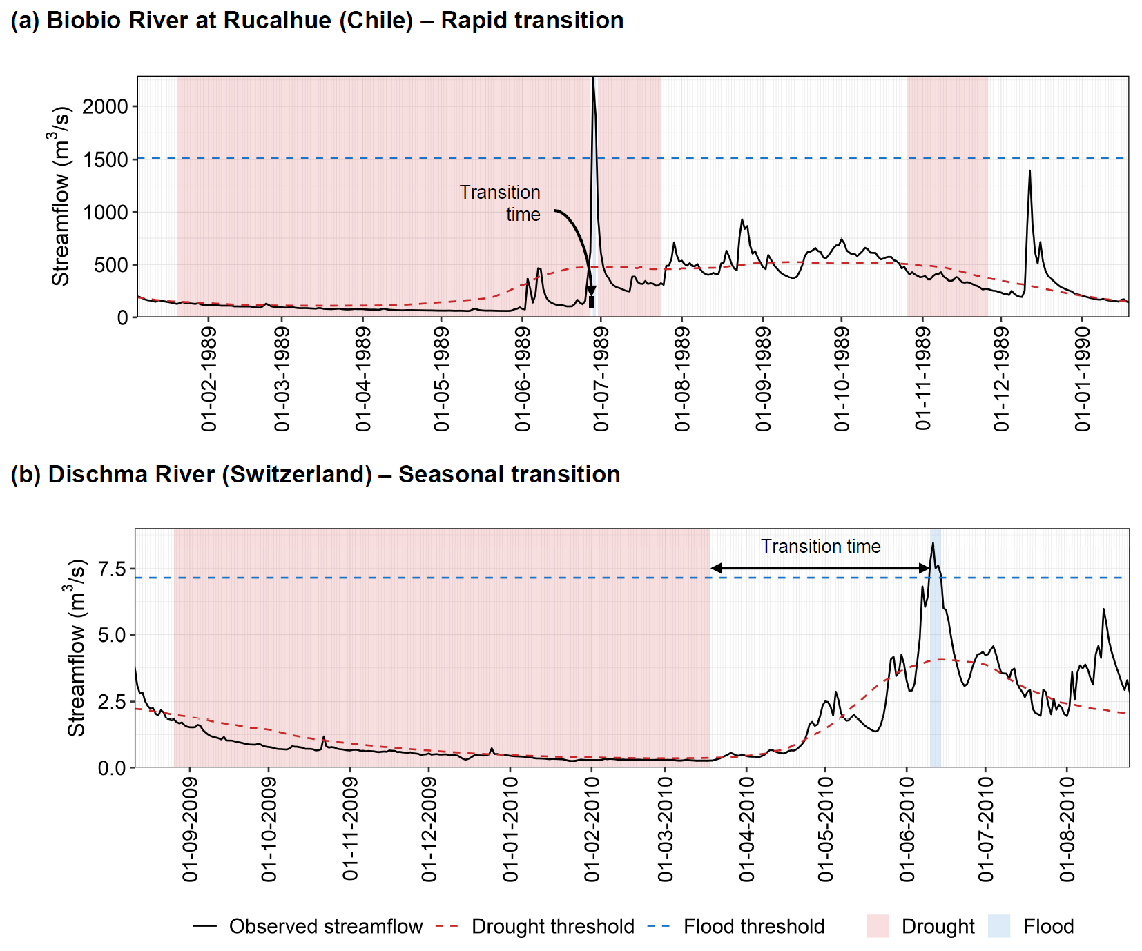
Figure 3 Example of the characterization of streamflow extremes and their transitions for two catchments within the study domain. (a) Biobio River at Rucalhue in Chile, and (b) Dischma River in Switzerland.

3.2 Modeling approach

3.2.1 Hydrological models

We use four conceptual bucket-style rainfall-runoff hydrological models: GR4J (Perrin et al., 2003), GR5J (Le Moine, 2008; Pushpalatha et al., 2011), GR6J (Pushpalatha et al., 2011), all coupled to the snow accumulation-ablation module CemaNeige (Valéry et al., 2014a, b), and TUWmodel (Parajka et al., 2007), which is based on the HBV model (Bergström and Forsman, 1973). All models have been widely used within the hydrological community during the last decades (Seibert and Bergström, 2022). GR4J, GR5J, and GR6J (with 6, 7, and 8 parameters coupled with CemaNeige, respectively; see Table S1 in the Supplement) were chosen to explore how slight changes in model structure affect simulated streamflow extremes, and the TUW model (with 15 parameters; see Table S2) was selected to explore how more complex models, in terms of the snow routine and the representation of the processes occurring in the production storage, simulate these phenomena.

Bucket-type conceptual models often include parameters and functions that allow for non-conservative adjustments to the water balance (i.e., artificially adding or leaking water). While they can help correct potential mismatches, e.g., between topographical and underground catchments, they can also compensate for biases in the forcing. To explicitly correct for biases in the meteorological forcings (as illustrated in Fig. 1c), two parameters were included in the calibration process in addition to the original setup for each hydrological model. Specifically, a multiplicative parameter for precipitation (dP) and an additive parameter for temperature (dT) were included to adjust systematic biases in precipitation and temperature.

The GR4J, GR5J, and GR6J models – hereafter referred to collectively as GRXJ for simplicity – share the same genealogy, meaning that they are based on the same core structure. These models can be coupled to the snow module CemaNeige, which partitions precipitation into liquid and solid precipitation and simulates snow accumulation and melt (rainfall and snowmelt enter the GRXJ structures). The basic structure of the GRXJ family corresponds to the GR4J model, which includes a parameter for production storage capacity, representing surface processes, and a parameter for routing storage capacity, representing subsurface processes. Additionally, GR4J includes an intercatchment exchange parameter and a unit hydrograph parameter that represents the delay between precipitation and streamflow. GR5J adds an additional parameter to the GR4J structure to improve the intercatchment exchange function, while GR6J includes a parameter for exponential storage in parallel to the routing storage included in GR4J and GR5J to improve the representation of groundwater processes (i.e., slow runoff). It is important to note that the original structure of GR4J cannot be recovered by setting the parameter X5 equal to zero in GR5J, nor can GR5J be obtained by setting parameter X6 = 0.01 (the minimum value that can be adopted) in GR6J. This is because, e.g., in GR5J the routing function differs from GR4J, whereas in GR6J the effect of the exponential storage (defined by X6) cannot be canceled. Thus, despite having the same core structure, the models are intrinsically different from each other.

The TUW model consists of a snow, soil, groundwater (subsurface flow), and a routing routine, similar to the HBV model (Bergström and Forsman, 1973). One of the major differences between the HBV and TUW models lies in their snow routines. The TUW model does not allow for meltwater or rainfall to be retained within the snowpack, nor does it account for the refreezing of liquid water. The snow routine partitions between liquid and solid precipitation and estimates snow accumulation and melt. Rainfall and snowmelt enter the soil routine, where actual evaporation, soil moisture, and recharge are estimated. Then, the recharge flow goes to the groundwater routine, represented by two storages that produce surface runoff and quick flow (upper), and baseflow (lower). The sum of these flows is delayed in the routing routine using a triangular transfer function. Unlike the GRXJ models, which follow a water balance approach to characterize the production storage, TUW estimates evapotranspiration and recharge based on an explicit conceptualization of soil moisture content.

While both CemaNeige and the snow routine implemented in the TUW model follow a degree-day factor approach, there are differences in (i) the characterization of the precipitation phase (TUW allows the existence of a mixed partition between rain and snow), (ii) the conditions for snowmelt (free parameter in the TUW model and set to 0 °C for CemaNeige), and (iii) the presence (or absence) of a parameter to correct for snowfall undercatch (not available in CemaNeige). These differences also explain the number of parameters that each of the snow routines has (two and five for CemaNeige and the snow routine in the TUW model, respectively).

Despite their structural differences and conceptualizations (for further details refer to Astagneau et al., 2021b), these models provide simplified representations of some hydrological states, fluxes, and processes at the catchment scale using precipitation (P), mean temperature (T), and potential evapotranspiration (PET) at daily time steps as inputs. To estimate PET, we used the approach proposed by Oudin et al. (2005), which is based on temperature and requires latitude and the day of the year as a proxy for extraterrestrial radiation. Additionally, as the snow module CemaNeige can be configured in a semi-distributed way, we discretized each catchment into equal-area elevation bands based on the hypsometric curve by considering 10 elevation bands for all evaluated model structures. To make simulations comparable across model structures, precipitation and temperature inputs for the TUW model were extrapolated through 10 elevation bands following the approach implemented in the GRXJ models, based on the orographic gradients defined by Valéry et al. (2010).

3.2.2 Calibration strategy

The parameters of each model structure, as well as the forcing adjustment parameters introduced, were calibrated using daily streamflow records and the Dynamically Dimensioned Search (DDS; Tolson and Shoemaker, 2007) over the period 2000–2020. This calibration period was defined to capture the current hydroclimatic conditions in the modeling setup. Note that, because the temperature-adjustment parameter was incorporated, potential evapotranspiration was recalculated at each evaluation run within the calibration algorithm to maintain consistency between the two variables. Additionally, following the traditional calibration approach proposed for GRXJ models (e.g., Pelletier and Andréassian, 2022), a parameter-space transformation is applied to improve the search process during calibration (details in Table S3).

Different objective functions based on the KGE configuration were used to calibrate each model. In its most general form, the KGE (Eq. 1) compares simulations to a reference based on three components, i.e., dynamics (e.g., correlation), variability (e.g., standard deviation), and bias (e.g., mean). KGE values range from negative infinity to one, which represents the optimum. How each component is defined depends on which KGE formulation is used. To the best of our knowledge, there exist five such formulations in the literature (Gupta et al., 2009; Kling et al., 2012; Pool et al., 2018; Tang et al., 2021; Pizarro and Jorquera, 2024, more details in Table 1). Additionally, different scaling factors or weights (i.e., c₁, c₂, and c₃ in Eq. 1) can be used to put more emphasis on some of the components of the KGE as well as different streamflow transformations to give more weight to specific parts of the flow distribution (e.g., Thirel et al., 2024; Mizukami et al., 2019). To emphasize low flows, for example, flows can be transformed to the inverse of streamflow (i.e., $\mathrm{1}/Q$; e.g., Garcia et al., 2017; Wu et al., 2025). Further, linear combinations of the KGE applied to flows with and without transformation (i.e., Q and $\mathrm{1}/Q$, respectively) have been presented as useful objective functions to find a good compromise between high- and low-flows (e.g., Araya et al., 2023; Knoben et al., 2020; Muñoz-Castro et al., 2023).

$$\begin{array}{}\text{(1)}& \text{KGE}=\mathrm{1}-\sqrt{\begin{array}{l}(c_{\mathrm{1}}\cdot (\text{dynamics}-\mathrm{1}){)}^{\mathrm{2}}\\ +(c_{\mathrm{2}}\cdot (\text{variability}-\mathrm{1}){)}^{\mathrm{2}}\\ +(c_{\mathrm{3}}\cdot (\text{bias}-\mathrm{1}){)}^{\mathrm{2}}\end{array}}\end{array}$$

For each hydrological model and catchment, 60 different objective functions were implemented based on the possible combinations of the following methodological choices: (i) 5 KGE formulations (Table 1), (ii) 3 streamflow transformation cases (High, Low, High-Low), and (iii) 4 weights applied to the variability term of the KGE (i.e., in Eq. 1, $c_{\mathrm{2}}=\mathrm{1},\mathrm{2},\mathrm{4},\mathrm{8}$). For the low-flow transformation (Low; i.e., using $\mathrm{1}/Q$), a constant equal to 1 % of the mean streamflow was added to the series to avoid zero-flow problems (see e.g., Pushpalatha et al., 2012; Garcia et al., 2017; Knoben et al., 2020). To facilitate the notation associated with the streamflow transformations tested here, we refer to the case as “Hi” (High) when a certain formulation of KGE was applied to untransformed streamflow (i.e., Q), while “Lo” (Low) refers to the case where a low-flow transformation was applied (i.e., $\mathrm{1}/Q$). We refer to the linear combination of both cases (i.e., $\mathrm{0.5}\times \text{Hi}+\mathrm{0.5}\times \text{Lo}$) as “HiLo”.

3.3 Model accuracy assessment

We assessed model accuracy both in terms of general model performance and the ability of the model to capture extreme events and the transitions between them. We followed a traditional split-sample test approach (Klemeš, 1986; Beven, 2025) to assess the general model accuracy over two time periods defined as (i) calibration (2000–2020) and (ii) evaluation (1985–1999). To test for general accuracy and hydrological consistency across the calibration experiments tested here, we computed several goodness-of-fit metrics (e.g., KGE) and hydrological signatures (e.g., seasonality, low- and high-flows). First, we assessed model performance across the 60 configurations by comparing the values obtained for each objective function during calibration. Second, we assess the predictive skill of our calibrated models by comparing their performance during calibration with that of a simple daily mean flow benchmark. This benchmark is defined as the mean flow for each day, calculated from all instances over the calibration period (referred as BM05 in Knoben, 2024). Third, we assessed model performance by looking at biases in a set of hydrological signatures, including seasonality, statistical properties (mean, variance), flow duration curve-derived signatures (e.g., mid-segment slope), and annual extremes (see Table S5). We conducted this analysis in two steps: (i) we analyzed the models' ability to reproduce the seasonal timing (seasonality) of streamflow (Q), snow water equivalent (SWE), and actual evapotranspiration (ET); and (ii) we computed biases in streamflow-derived signatures. The results of this general model performance assessment are presented in Supplement Sect. S1.

To assess the model's capability to detect streamflow extremes and their transitions, we used the Critical Success Index (CSI; Eq. 2), which is formulated based on the number of hits (H; events identified both in the reference/observations and the simulations), misses (M; events only identified in the reference/observations), and false alarm events (F; events identified only in the simulations). The CSI values vary between zero and one, with one representing the optimum. We defined hits as simulated events overlapping at least 50 % of the time window with their observed counterparts. Additionally, a tolerance window of 30 and 5 d was defined before the onset and after the end of an observed drought and flood event, respectively. In short, we aimed to evaluate the models' ability to capture streamflow extremes and their transitions rather than their characteristics (e.g., cumulative deficit during the drought period, flow peak, etc.).

$$\begin{array}{}\text{(2)}& \text{CSI}=H/(H+M+F)\end{array}$$

3.4 Assessment of the relative importance of modeling decisions

To assess the relative importance of modeling decisions on the detection of streamflow extremes and their transitions, we conducted an analysis of variance (ANOVA; Fisher, 1992; Kaufmann and Schering, 2014). The ANOVA enabled us to examine the relationship between different modeling decisions (e.g., choice of structure and different decisions related to calibration) and quantify their relative importance in explaining the total variance in the target variable (e.g., CSI). Thus, by dividing the total variance into different groups, genuine sources of variation that are not explained by chance can be identified. We assumed that the total variance (TV) in the target variable can be mainly explained by the differences between hydrological models (HM), KGE formulations (KGEf), streamflow transformations (QTR), and KGE component weights (W). If, for example, weights do not have a significant impact on the detection of streamflow extremes, we would expect a low value for the term “W”, that is a lower relative importance (i.e., $W/\text{TV}$) for explaining the total variance with respect to other decisions. Based on this conceptualization and considering a residual term (RS) that groups all the interactions between decisions and the variance that we cannot explain from them, the ANOVA can be expressed as follows:

$$\begin{array}{}\text{(3)}& \text{TV}=\text{HM}+\text{KGEf}+\text{QTR}+W+\text{RS}\end{array}$$

We also analyze the relative importance of the differences between catchments by including them in the ANOVA test. However, we ultimately removed this component from the explanatory variables because its influence sometimes dominated the results, thereby hiding the contribution of the intrinsic modeling decisions being tested to the variability observed in the CSI values.

3.5 Identification of important processes in simulating drought-to-flood transitions

To identify the most important processes in simulating drought-to-flood transitions, we assessed which model parameters explain the detection of events. To do so, we analyzed the relative importance of each model parameter in estimating the CSI through an ANOVA test applied per catchment. This analysis, expressed by Eq. (4), considers the 60 alternative configurations (i.e., parameter sets) available per model and catchment and uses the total variance explained (TV) by each parameter (θ_i; where $i=\mathrm{1},\mathrm{\dots },N_{\mathrm{p}}$, and N_p is the number of parameters) as a proxy for the importance of the associated variable/process in explaining event detection. The approach used to analyze the relative importance of the parameters explaining the variance of the CSI may have problems if the parameters do not show enough variation between the different configurations. However, despite the similarities in the configurations used for calibration, almost all the parameters show high variability among the calibrated parameter sets per catchment (see Fig. S15).

$$\begin{array}{}\text{(4)}& \text{TV}=\sum _{i=\mathrm{1}}^{N_{\mathrm{p}}}{\mathit{\theta }}_i+\text{RS}\end{array}$$

4 Results

4.1 General model performance assessment

Before looking at model performance in terms of capturing extreme events, we assessed the overall performance of the four models used. For this, we independently evaluated the calibration results for each configuration. Our results shown comparable performance across the hydrological models evaluated here (Fig. S1). For instance, all configurations outperform the defined daily mean flow benchmark (see Fig. S2), indicating that our models have greater predictive power with respect to the long-term observed streamflow series. Our more detailed analyses show that the seasonality of variables such as streamflow, SWE, and ET are simulated accurately, with median performance values across catchments and configurations between 0.79–0.98 (with 1.0 being the optimum). However, our evaluation shows that using weights for the variability term of KGE greater than 2 can be detrimental to the overall performance of the model, both in terms of representing the seasonality of the aforementioned variables (Fig. S3) and some hydrological signatures such as the high- and low-segments of the slope in the flow duration curve (FDC, Fig. S4). In general, the use of flow transformations yields values that are consistent with what the application seeks to capture (e.g., low-flows are better simulated with “Lo” transformation and high-flows are better simulated without transformation; see Fig. S5). There is little difference between different models and KGE formulations when weights and the HiLo transformation are used (Fig. S6). Considering those configurations with comparable performance (i.e., removing those relying on weights greater than 2), average accuracy across configurations ranges between 0.87–0.92, 0.88–0.93, and 0.75–0.85, for the high-, mid-, and low-segment of the slope of the FDC, respectively. Further details on overall model performance are presented in Sect. S1.

The results presented subsequently are based on the simulations with the HiLo (i.e., $\mathrm{0.5}\times \text{KGE}\left(Q\right)+\mathrm{0.5}\times \text{KGE}(\mathrm{1}/Q)$) configuration, except for specific cases for which all 30 configurations (i.e., removing weights greater than two) per catchment were used (e.g., ANOVA tests). Previous studies have already shown that the use of this configuration results in a good compromise between simulating low and high flows (e.g., Garcia et al., 2017; Thirel et al., 2024; Lema et al., 2025).

4.2 Suitability of KGE for calibrating models aimed at simulating drought-to-flood transitions

Next, we assess how strongly the general model performance described by the KGE is linked to the capability of the model in detecting extreme events. To do so, we compared the objective function value retrieved for one of our calibration configurations – the original KGE formulation configured with unweighted HiLo (i.e., c₂=1 and HiLo = $\mathrm{0.5}\times \text{KGE}\left(Q\right)+\mathrm{0.5}\times \text{KGE}(\mathrm{1}/Q)$), which is later used as a reference – with the performance in detecting droughts, floods and their transitions based on the CSI (Fig. 4). Our comparison clearly shows that model performance varies across catchments and model structures for both the KGE and CSI. While the overall performance described by the KGE can potentially be used as a proxy for a model's performance in capturing droughts for some catchments (e.g., points close to the optimal values for both KGE and CSI, i.e., 1, and CSI ranges from 0.18 to 0.74 for GR4J and from 0.18 to 0.78 for TUW), this link between general model performance and event detection is neither generalizable to floods and transitions, nor to all the models tested here. Rather, a high KGE does not necessarily imply a high CSI for these two types of events.

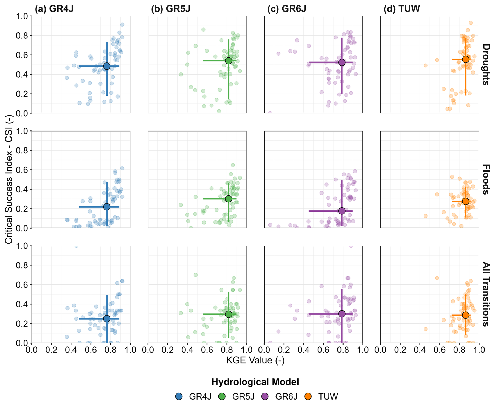
Figure 4 Comparison between the Kling–Gupta Efficiency (KGE) for the calibration period and the Critical Success Index (CSI) for droughts, floods, and transitions, based on the simulations with the models (a) GR4J, (b) GR5J, (c) GR6J, and (d) TUW calibrated with the unweighted original KGE formulation as the objective function. The dispersion bars are associated with the 10th and 90th percentiles across catchments, while the central shape indicates the 50th percentile. Transparent circles show results for each catchment. For both KGE and CSI, the optimal value is 1.

While KGE is not necessarily a good proxy for how well a model captures extreme events (especially floods and transitions), some specific KGE formulations might be better suited for this task than others. We evaluate this in a next step by exploring to what extent different adjustments in the “basic” configuration used for the analysis presented above can (or cannot) improve the performance in detecting streamflow extreme events and, particularly, drought-to-flood transitions.

4.3 Impacts of KGE configurations on drought-to-flood transition simulations

To assess the added value of the application of weights to the variability term of the KGE as well as the use of different KGE formulations for detecting independent extreme events and their transitions, we use the GR4J model as an example to quantify differences in CSI between the unweighted original KGE (reference) and alternative cases (e.g., weights and/or KGE formulations; Fig. 5). We find that, in the context of a large-sample study, weighting the variability term of the KGE does not consistently enhance model performance in detecting streamflow extremes and their transitions (median difference is centered around 0 in both cases) and may even be detrimental. Further, weighting the variability term can substantially worsen flood detection (e.g., GRXJ models, Fig. S10). Additionally, we find that using a modified KGE formulation, rather than the original, does not substantially improve model performance. In short, the use of weights and the choice of the KGE formulation do not play a dominant role in the overall performance of the model over the study domain. These findings are consistent across the other model structures tested (see Fig. S10).

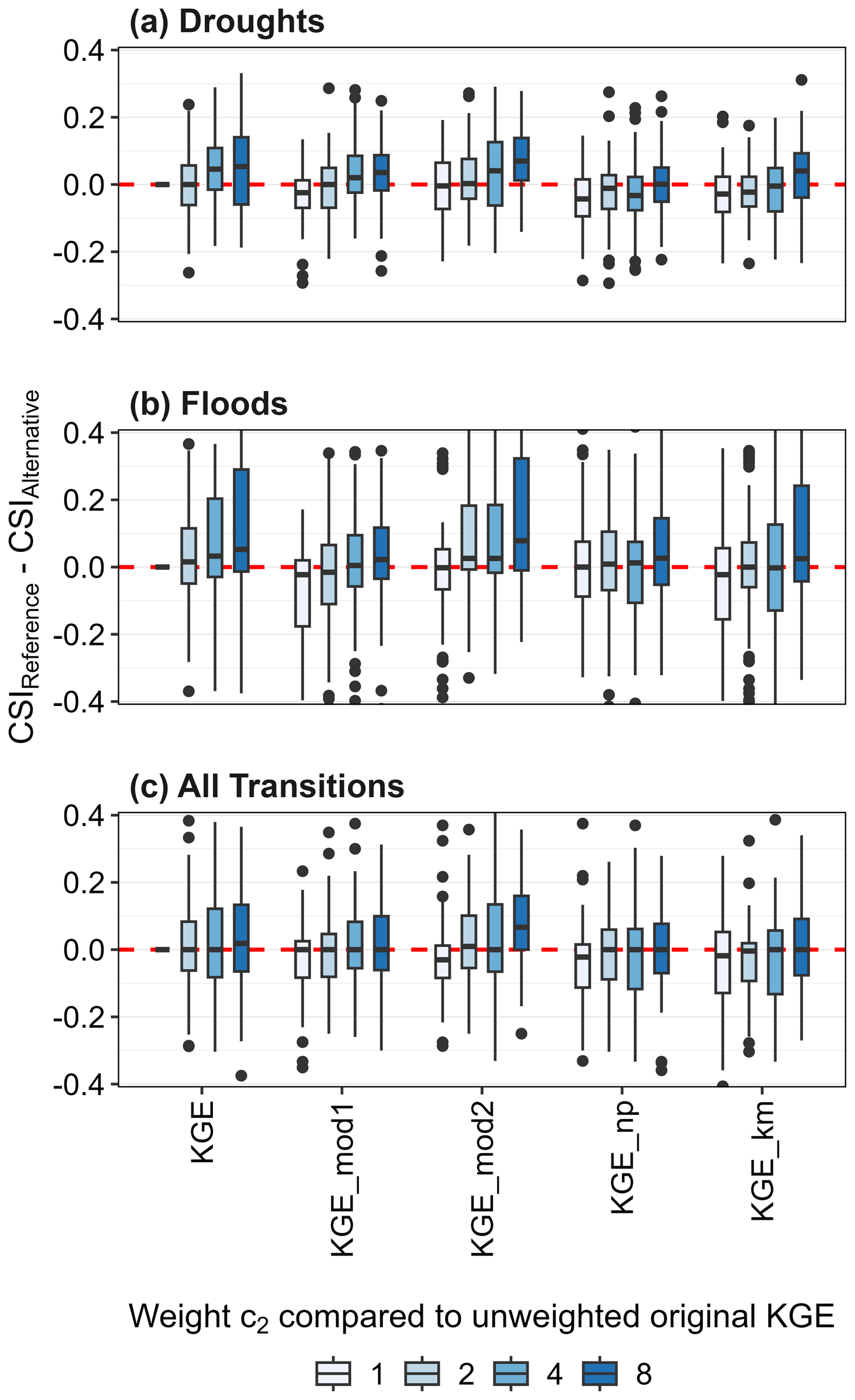
Figure 5 Difference in the CSI for GR4J simulations obtained using model calibrations with no weights and the original KGE (reference) versus different weights and KGE formulations (alternative) for (a) droughts, (b) floods, and (c) transitions. Values above (below) 0 indicate better (worse) performance of the reference compared to the alternative. Each boxplot displays the information of 63 values (i.e., one per catchment).

4.4 Importance of model structure

Our results show that drought detection is typically more reliable than that of floods and transitions between the two (Fig. 6). However, there are no significant differences in the detection rate of droughts, floods and their transitions, across the hydrological models. While the CSI median values slightly improve when switching from the GR4J model to the other GRXJ and TUW versions for droughts (0.49 to 0.55), this is not the case for floods and transitions. For instance, for floods, GR5J stands out among the GRXJ models (CSI = 0.30, compared to 0.22 and 0.18 for GR4J and GR6J, respectively), while for transitions, GR6J shows a better performance compared to the simpler models (CSI = 0.30, compared to 0.25 and 0.29 for GR4J and GR5J, respectively). This suggests that adding more parameters does not necessarily lead to improved model performance when detecting extreme streamflow events.

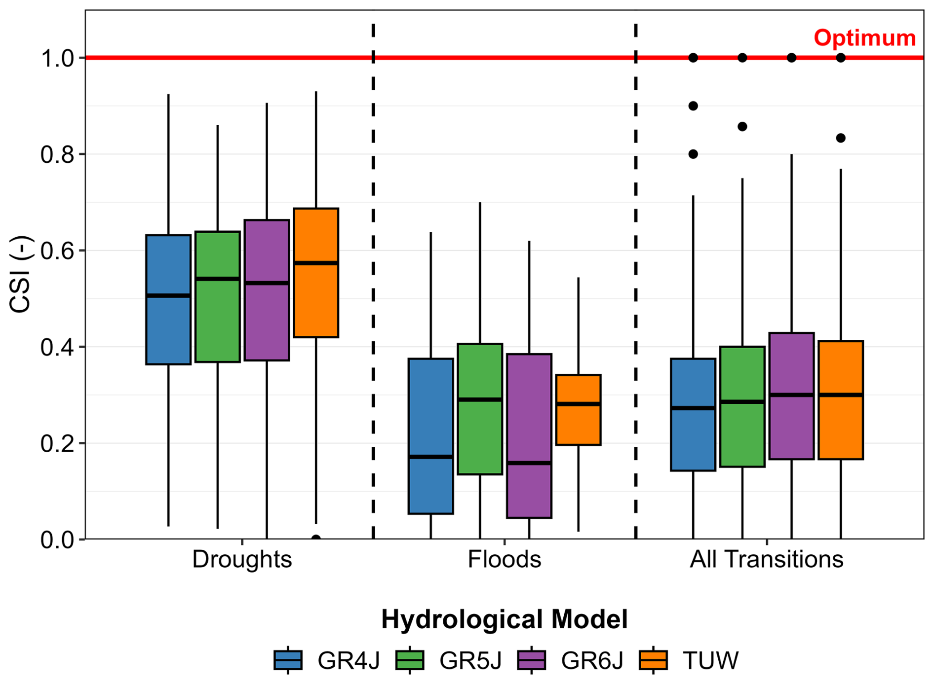
Figure 6 Critical Success Index (CSI) for (a) droughts, (b) floods, and (c) drought-to-flood transitions, based on the simulations with GR4J, GR5J, GR6J, and TUW (different colors) calibrated with the unweighted HiLo original KGE formulation as the objective function. Each boxplot displays the information of 63 values (i.e., one per catchment).

These results hold independently of the country considered (see Fig. S11 for a comparison between Swiss and Chilean catchments). However, the detection of extreme events is more challenging in catchments located in Chile compared to those located in Switzerland, with differences in the median CSI between countries (i.e., CSI_CH−CSI_CL) lying around 0.28, 0.12, and 0.16 for droughts, floods, and drought-to-flood transitions, respectively.

Different model structures can result in similar streamflow simulations even though they represent hydrological fluxes and states in different ways. To illustrate this, we compare simulated fluxes obtained for an observed seasonal drought-to-flood transition in the Dischma river in Switzerland across the four hydrological models (Fig. 7). While three out of four models capture the transition event successfully (GR6J fails in capturing its timing) and show similar temporal patterns of ET, snowmelt, and SWE, the contribution of baseflow (presented as a percentage of total runoff) varies strongly among them. Consequently, the analysis of the drivers associated with such transition events will vary depending on which model structure is analyzed. Although there is a high agreement between the models in terms of the detection of the event in this sample case (i.e., 3 out of 4), such agreement is not necessarily apparent for all events and catchments (Fig. 4).

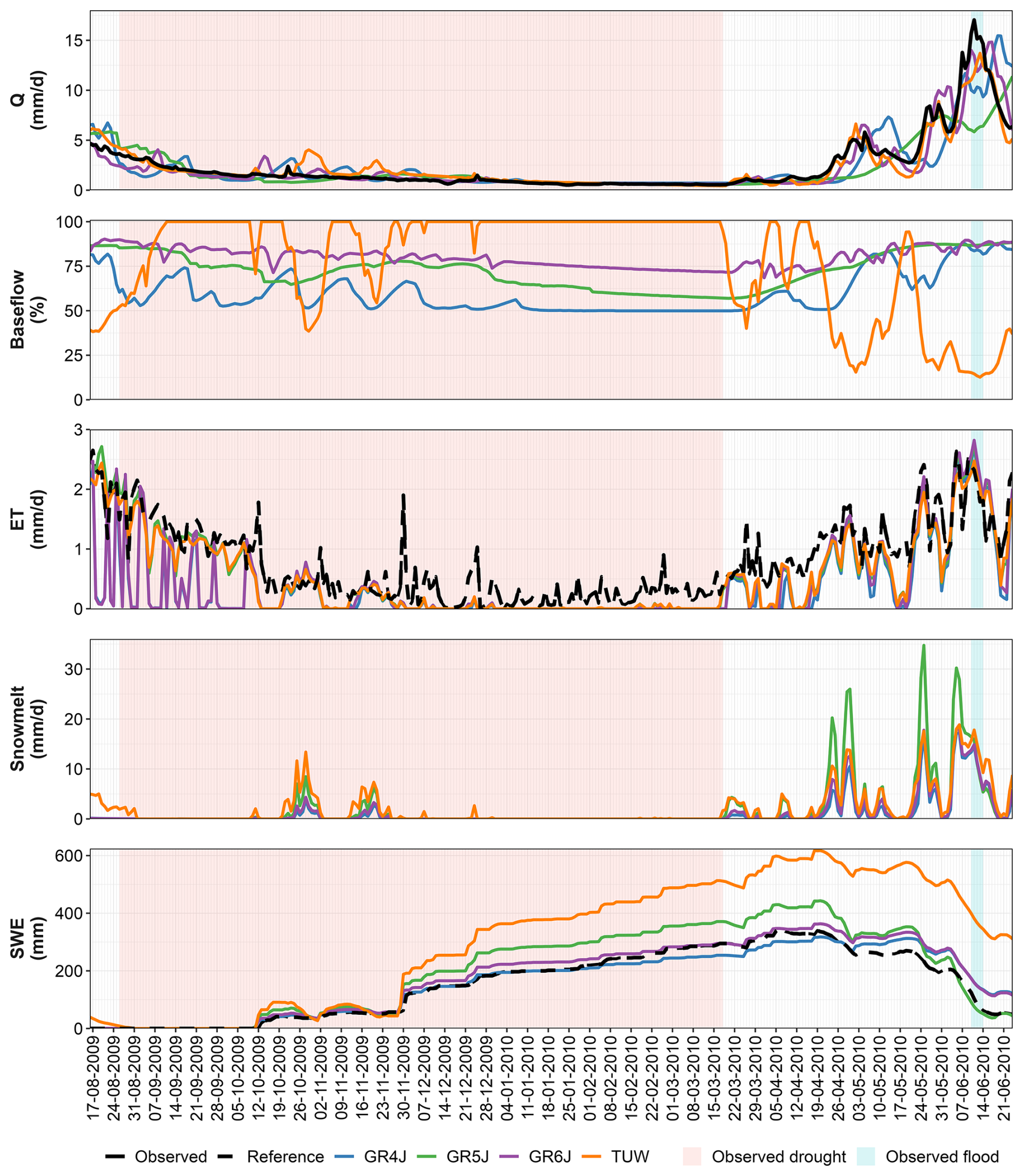
Figure 7 Example of how different hydrological fluxes and states – such as runoff (Q), baseflow, actual evapotranspiration (ET), snowmelt, and snow water equivalent (SWE) – are simulated for an observed drought-to-flood transition in the Dischma river (Switzerland) with the GR4J, GR5J, GR6J, and TUW hydrological models calibrated with the unweighted HiLo original KGE formulation.

4.5 Relative importance of different modeling decisions

Our previous results showed no significant differences when pooling results by model (Fig. 6). However, when it comes to the relative importance in explaining the total variance of the detection skill, the results of the ANOVA show that the most important modeling decision in simulating extreme events and their transitions is the choice of a suitable model structure, followed by the choice of the streamflow transformation (Fig. 8). In contrast, the choices of KGE formulation and weights do not have a strong impact on the performance in simulating streamflow extremes. For floods, the transformation is more important because of the loss of performance in representing high flows when the model is calibrated with a low-flow transformation (Fig. S5). This highlights the importance of selecting the appropriate transformation according to the modeling objectives. Additionally, when catchment characteristics are included as an explanatory variable, they strongly influence drought detection, while they have little effect on flood detection (see Fig. S13). The relative importance of the methodological choices is similar when analyzing other categorical indices, such as the probability of detection, false alarm ratio, and frequency bias (see Fig. S12).

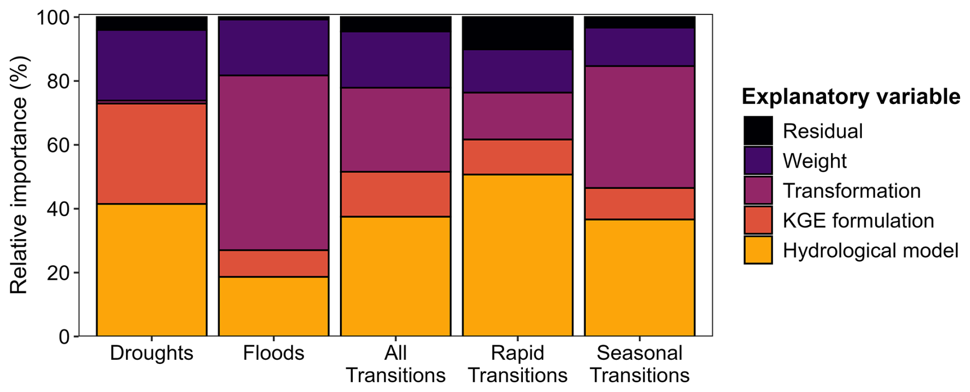
Figure 8 Results of the analysis of variance (ANOVA) applied to the Critical Success Index (CSI) for droughts, floods, all drought-to-flood transitions (i.e., rapid and seasonal), rapid transitions (< 14 d), and seasonal transitions (< 90 d).

4.6 Model accuracy depends on catchment characteristics

We further explore the relationship between model accuracy and catchment characteristics using Spearman's rank correlation coefficient. To this end, we focus on the CSI obtained for the different types of extreme events of interest (droughts, floods, and transitions) generated with the GR4J and TUW models calibrated with the unweighted HiLo original KGE formulation (Fig. 9; extended version including all models in Fig. S14). Drought-to-flood transitions are more difficult to capture in semi-arid (negative correlation between aridity index and CSI), high-mountain (negative correlation between mean elevation and CSI), and flashy (negative correlation between the slope of the flow duration curve and CSI) catchments than in humid low-elevation catchments with high streamflow elasticity to precipitation (Fig. 9). This result is generalizable to the other models and the different KGE formulations tested (see Fig. S14).

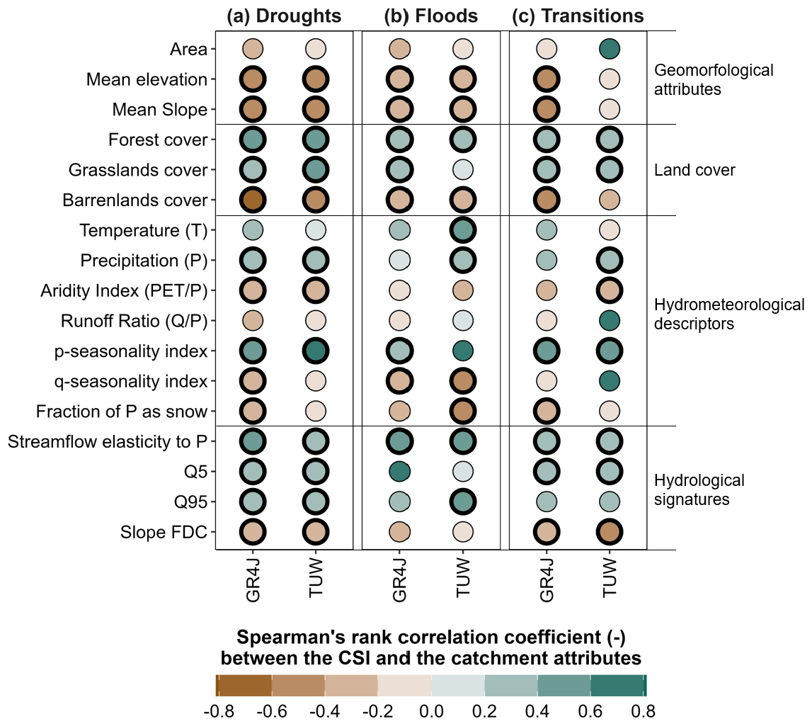
Figure 9 Spearman's rank correlation coefficient between different catchment attributes and the CSI for (a) droughts, (b) floods, and (c) drought-to-flood transitions, based on the simulations with GR4J and TUW calibrated using the unweighted HiLo original KGE formulation as the objective function. The circles with thick outlines indicate correlation coefficients with p-values lower than 0.05.

4.7 Linking model performance to hydrological processes during streamflow extremes

We conduct an ANOVA test to analyze the relative importance of different model parameters in detecting streamflow extremes and their transitions (Fig. 10; the extended version with rapid and seasonal transitions is presented in Fig. S18). We show that some model parameters are relatively more important than others (e.g., X4 for floods in GRXJ models), but that the relative importance of a given parameter can vary substantially across catchments. All of the hydrological models show a high importance of the parameters aimed to adjust the forcings (i.e., dP and dT for all the models as well as SCF in TUW model, which seeks to correct for the snow undercatch). For the GRXJ models, X3 (routing store capacity) and X4 (unit hydrograph time constant) are most important in the simulation of low and high flows compared to the rest of the parameters, which is accentuated when more complexity is added to the base structure (i.e., GR6J). In the TUW model, which has more parameters than the GRXJ structures, the relative importance of each parameter is more uniform, and their relative importance is low, except for the parameter k0 (storage coefficient for very fast response), which becomes more important for flood detection in comparison to, e.g., drought detection.

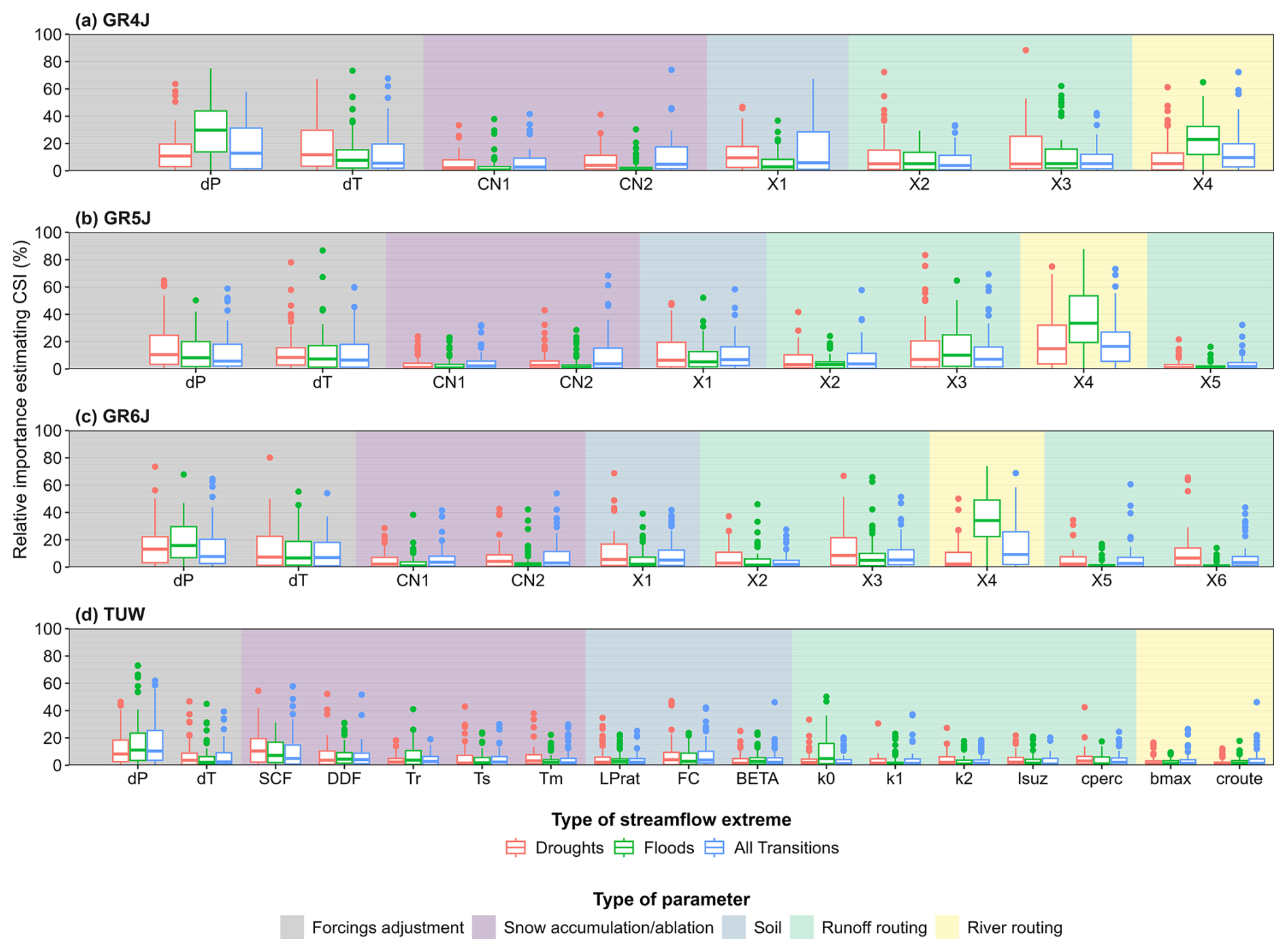
Figure 10 Relative importance of parameters for explaining the Critical Success Index (CSI) for models (a) GR4J, (b) GR5J, (c) GR6J, and (d) TUW based on the results of an analysis of variance (ANOVA).

5 Discussion

5.1 Simulation of compounding streamflow extreme events

We find that the hydrological models tested are better at detecting droughts (median CSI across catchments and KGE formulations: 0.50–0.58) than floods (median CSI across catchments and KGE formulations: 0.13–0.34), and their performance in detecting drought-to-flood transitions is closely related to (and likely limited by) their performance in detecting floods (0.25–0.33; Fig. 4). This difference in drought and flood simulation performance can be attributed to the different timescales associated with these two types of extreme events: while droughts vary in duration from months to years (or decades), floods develop, and may also subside, in a matter of hours or days. This is consistent with the poor performance of all the models tested in capturing rapid transitions (i.e., occurring within 14 d). Moreover, we obtained CSI values greater than zero for rapid transitions only in 13 basins (not shown). Overall, our analyses highlight that these fast processes are rather difficult to capture in conceptual rainfall-runoff models like GRXJ and TUW.

5.2 Good general model performance does not imply that extremes are well detected

Our results highlight that a good general model performance in terms of KGE does not necessarily imply a good performance in detecting streamflow extremes. Even models with high accuracy, measured by traditional metrics such as KGE, struggle to capture extreme events, particularly floods and transitions from drought to flood (Fig. 4). These findings are aligned with previous studies discussing the potential of KGE to represent high-flow values or capture flashy streamflow dynamics (e.g.,  Astagneau et al., 2022; Brunner et al., 2021; Mathevet et al., 2020). For instance, from a modeling perspective, Astagneau et al. (2021a) demonstrated that the relationship between KGE values and a model's capability in simulating summer floods is weak. Similarly, Bruno et al. (2024) showed that, during extreme low-flow conditions, model performance is usually lower than during normal flow conditions. Spieler and Schütze (2024) showed that the KGE lacks the capacity to provide information about detailed processes, leading to gaps between model accuracy (i.e., how well a model matches simulations with observations) and adequacy (i.e., how well a model captures key processes and behaviors of the observed system). These findings suggest that the traditional evaluation of hydrological models through goodness-of-fit metrics such as KGE or NSE must be accompanied by an explicit examination of their capability to simulate and detect streamflow extreme events, e.g., by using metrics such as the CSI.

From a process perspective, hydrological model underperformance can be linked to oversimplified or poorly represented (or understood) processes (Beven, 2019; Clark et al., 2017; Hrachowitz et al., 2014; McMillan et al., 2018). For instance, in the context of drought-to-flood transitions, prolonged dry conditions can alter soil properties, such as cracking (Gimbel et al., 2016; dos Santos et al., 2016), water repellency (Doerr et al., 2007; Leighton-Boyce et al., 2007), and macropore connectivity (Or et al., 2013), changing the infiltration-runoff partitioning and potentially intensifying catchment responses to precipitation. Despite their importance for flood generation, these soil and near-surface processes remain poorly understood and, consequently, are rarely represented in conceptual or even physically-based hydrological models (Brunner, 2023; Barendrecht et al., 2024; Blöschl et al., 2019). This limits their ability to reproduce streamflow extremes, such as droughts and floods, and rapid shifts between them. Therefore, it is important to improve our understanding of the processes behind transitions and how they are represented in hydrological models.

5.3 The importance of different modeling decisions for simulating streamflow extremes and their transitions

Our results show that model structure is the most important modeling decision for capturing extreme events and their transitions (Fig. 8), which is consistent with previous studies focused on the independent analysis of extreme events (e.g., Alexander et al., 2023; Melsen and Guse, 2019; van Kempen et al., 2021). Among the structures tested, slight but non-significant differences were found in terms of their performance in representing streamflow extreme events (Fig. 6). However, there is an evident decrease in performance in detecting floods compared to droughts, which generalizes across the four models tested. These deficiencies in flood simulation performance translate to deficiencies in capturing drought-to-flood transitions (Figs. 4 and 6). These findings suggest that the lack of an explicit structural component allowing for the simulation of floods that occur under dry and low soil moisture conditions could explain the poor performance associated with this type of compound event. Indeed, Astagneau et al. (2022) highlighted that conditioning the storages and fluxes of a lumped conceptual hourly-timestep model on rainfall intensities could benefit model performance in catchments with a fast response to precipitation (i.e., flashy-catchments). For droughts, van Kempen et al. (2021) have shown that the magnitudes of the low-flow events are significantly affected by alterations in the architecture of the upper and lower storages, which is consistent with the changes in performance among the GRXJ models (Fig. 6), where small structural modifications lead to changes in the detection of these events.

We demonstrated that the capability of a model to identify streamflow extreme events and their transitions in simulations varies depending on its structure. In contrast, model accuracy in detecting extreme events does not necessarily depend on the number of model parameters (Fig. 6). Several studies have highlighted that including a more detailed representation of hydrological processes in models does not necessarily imply better accuracy (e.g., Orth et al., 2015; Valéry et al., 2014a). This is because more realistic representations require more detailed information to characterize the system of interest (e.g., land cover maps, distributed forcings, a high-resolution digital terrain model, soil properties), which are not always available. Recently, Santos et al. (2025) found that models with varying complexity can lead to similar robustness issues, stressing the need to improve strategies for diagnosing the suitability of model structures to improve the understanding of specific hydrological processes (e.g., Spieler and Schütze, 2024; Knoben et al., 2020).

The results presented here show that the choice of objective function is relatively less important compared to the choice of model structure (Fig. 8). However, choosing an appropriate transformation can be an important decision for improving a model's ability to capture flood events. Model performance can be optimized both in terms of general performance and the representation of extreme events (CSI) under (a) the application of equal weights to all components of the KGE (Fig. 5) and (b) the application of a streamflow transformation that focuses on both high and low flows (Figs. S1–S6). Our comparison also highlights that the potential benefit from adjusting these choices (e.g., using other weights or other transformations) varies widely between catchments (Fig. 5). This is in line with the findings of Mizukami et al. (2019), who found that the influence of weights on model performance depends on model structure and catchment characteristics. While none of the tested modifications in the objective function consistently improve the simulation of streamflow extremes across all catchments in the study domain, some of the alternative KGE formulations could improve the simulation of certain variables in certain catchments.

The high relative importance of the forcing adjustment parameters for event detection (i.e., dP and dT for all the models as well as SCF in TUW model, which seeks to correct the snow undercatch; Fig. 10) suggests that the meteorological forcings can have a major impact on the detection of streamflow extremes and their transitions. Several studies have shown that errors in meteorological forcing are a key challenge in hydrological modeling (e.g., Brunner, 2023; Döll et al., 2016) due to, e.g., their large influence on the simulation of snow processes (e.g., Tang et al., 2023; Günther et al., 2019), or significant impacts on the partitioning between evaporation and runoff (e.g., Nasonova et al., 2011). Here, we attempt to reduce this effect by (1) preferring local meteorological products over global ones (e.g., Clerc-Schwarzenbach et al., 2024), and (2) incorporating adjustment factors to account for potential systematic biases associated with them (e.g., Hughes, 2024; Probst and Mauser, 2022). However, introducing forcing adjustment factors could artificially compensate for some model deficiencies by modifying the inputs (e.g., Tang et al., 2023, 2025). This is evidenced by the high dispersion of forcing adjustment factors within each configuration (Fig. S16) where, e.g., catchments with higher precipitation falling as snow tend to have higher values in precipitation adjustment. We acknowledge that the incorporation of forcing adjustment parameters could have an impact on the partitioning of precipitation between ET and runoff. However, this problem also occurs when working with different parameter sets, which may come from different calibration functions. We have evaluated the impact of incorporating these additional parameters on the identifiability of the original model parameters, showing that there are no meaningful impacts (see Fig. S19). In light of these findings, we surmise that improvement in the spatiotemporal representation of precipitation and temperature, as well as of the potential interactions between these variables, might represent a critical step towards improved representations of compound streamflow extreme events in hydrological models.

5.4 Limitations and recommendations for future work

Our model calibration experiments focused on the simulation of extreme streamflow events, which required the choice of specific event definitions. Here, we defined hydrological droughts and floods using threshold-based approaches, and the thresholds were adjusted in a way to identify, on average, one event per year and catchment. Because this methodological choice does, to a certain degree, affect the outcomes of the comparison, we tested different thresholds for defining streamflow extreme events. The results of this sensitivity analysis indicate that using more flexible thresholds to define droughts (i.e., higher percentiles) can enhance the detection of these events, as more instances are identified, and they tend to be less severe compared to more restrictive thresholds (see Fig. S8). The improvement in drought detection when the threshold is relaxed can be explained by the fact that models generally struggle during more extreme hydrological drought periods (e.g., Bruno et al., 2024), which are relatively less frequent if the threshold is raised. However, we did not find such an effect for floods and transitions, for which we obtained similar model performances regardless of the thresholds used (see Fig. S8). Similar results are obtained when the overlap window used to identify the hits is modified (Fig. S9). While our study shows that the choice of threshold does not substantially affect model accuracy in terms of transition events, the method used to define streamflow extreme events can have a major impact on the characteristics of the transition events identified.

To support our analysis, we tested four bucket-type hydrological models used within the hydrological modeling community (Addor and Melsen, 2019). Even though these models are at the lower end in terms of model complexity (Hrachowitz and Clark, 2017), and three of them share the same core structure, they allowed us to perform a comprehensive analysis of different model structures at a lower computational cost than when using models with more complex structures (e.g., Clark et al., 2017; Orth et al., 2015; Poncelet et al., 2017). Furthermore, previous studies have also shown that more complexity does not necessarily imply better performance (Fig. 6; e.g., Li et al., 2015; Merz et al., 2022).

These models have been calibrated based on daily streamflow records, using different objective functions derived from KGE formulations, and considering the set of parameters with the best performance as the optimum. However, it is important to acknowledge that potential compensations for biases in meteorological forcings or model deficiencies can make the “optimal” parameter sets less identifiable (e.g., Clark and Vrugt, 2006; Vrugt et al., 2005; Beven, 2025). Here, we explore the (dis)agreement between the optimal parameters for each configuration (Fig. S17), showing overall agreement indices of around 0.5 (i.e., the parameters have a range of variation of approximately 50 % of the parameter space). Based on the evaluation of the models' performance, we were able to verify that, despite the dispersion of optimal parameters, the simulations are consistent with the products used to evaluate the models (Figs. S3 and S6). To (i) complement model assessment, (ii) better define the parameter exploration range, and (iii) lead to parameter sets that ensure reliability and fidelity in representing hydrological processes, hydrological variables other than streamflow, such as SWE or ET, can provide useful information to improve hydrological modeling.

Our results provide insights on possible avenues of future research that could benefit drought-to-flood transitions modeling, which include: (1) exploring the use of modular platforms and a multi-model ensemble approach to quantify model uncertainty and identify more suitable model structures (e.g., Saavedra et al., 2022); (2) improving our understanding of the role of the spatial variability of precipitation for accurate flood simulations (e.g., Macdonald et al., 2025; Astagneau et al., 2022); (3) assessing the benefits of model runs at a subdaily timestep (e.g., hourly); and (4) exploring alternative data-driven modeling approaches such as long short-term memory (LSTM) networks (e.g., Frame et al., 2022; Acuña Espinoza et al., 2025; Kratzert et al., 2018).

6 Conclusions

We performed a modeling intercomparison study to (i) explore to what extent hydrological models can simulate drought-to-flood transitions and (ii) identify suitable modeling choices aimed at capturing these compound extreme events. For this intercomparison, we calibrated four conceptual bucket-type hydrological models (GR4J, GR5J, GR6J, and TUW) for 63 catchments in Chile and Switzerland using 60 different configurations of the Kling–Gupta Efficiency (KGE) as objective functions, based on five KGE formulations, four scaling factors, and three streamflow transformations. Based on the results of this intercomparison, we draw the following conclusions:

1. A satisfactory general model performance, as expressed by the KGE, does not guarantee a good performance in terms of detecting streamflow extremes and their transitions. While KGE can serve as a rough proxy for low-flow performance, it cannot for high-flows and drought-to-flood transitions. Consequently, assessments of the suitability of hydrological models for simulating extreme events and their transitions should use metrics capable of directly quantifying performance in terms of capturing extreme events, such as the critical success index (CSI).

2. The most important modeling decision when it comes to simulating floods, droughts, and their transitions is the choice of a suitable model structure. However, in a large-sample context, we demonstrate that the four models tested here (i.e., GR4J, GR5J, GR6J, and TUW) have similar performance, showing that adding more parameters does not necessarily improve the representation of extreme events.

3. In contrast, despite it still playing a large role in floods, the choice of the objective function and its exact configuration are, overall, less important. The choice of a suitable streamflow transformation can improve the simulation of extreme events to a certain degree. Specifically, a joint focus on high and low flows by equally weighting the two streamflow transformations in the objective function (referred to as HiLo in our analysis) can improve model performance without compromising its ability to capture streamflow extremes. However, the choice of the exact KGE formulation and the use of weights for the variability term of the KGE do not substantially affect the simulation of extreme events and the direction of this effect depends on the catchment.

4. Drought-to-flood transitions are more difficult to capture in semi-arid, high-mountain catchments than in humid low-elevation catchments.

5. Overall, simulation of both high and low streamflow extremes (i.e., those associated with floods and droughts), as well as transitions between them, remains challenging. This appears to be especially true for floods and drought-to-flood transitions. This may complicate interpretation of hydrologic response to increasingly volatile hydroclimate forcings in a warming world, and suggests that new modeling methods may be required to better understand extremes and their transitions amid climate change.

This methodological intercomparison highlights that simulating streamflow extremes and their transitions is not a trivial modeling task and continued research is needed to improve model accuracy for compound events. The results of this intercomparison study suggest that time is best invested when focusing on improving model structures rather than calibration procedures. Specifically, hydrological model development should focus on improving the representation of processes and components associated with the temporal dynamics of discharge, such as routing or the soil response to intense snowmelt and rainfall. Additionally, the strong link between model accuracy and parameters aimed at correcting precipitation inputs suggests that the representation of extreme events can be improved by investing in the quality of meteorological forcing datasets. Investments in improving the simulation of extreme events and their transitions are crucial because hydrological models can not only support process understanding related to compounding streamflow extremes, but can also be used to forecast such events at short time scales and to project future changes in the occurrence of drought-to-flood transitions. Such applications are critical to ensure society's preparedness for these types of hydrometeorological extreme events.