AI image-based method for a robust automatic real-time water level monitoring: a long-term application case

The study presents a robust, automated camera gauge for long-term river water level monitoring operating in near real-time. The system employs artificial intelligence (AI) for the image-based segmentation of water bodies and the identification of ground control points (GCPs), combined with photogrammetric techniques, to determine water levels from surveillance camera data acquired every 15 min. The method was tested at four locations over a period of more than 2.5 years. During this period almost 218 000 images were processed. The results demonstrate a high performance, with mean absolute errors ranging from 0.96 to 2.66 cm in comparison to official gauge references. The camera gauge demonstrates resilience to adverse weather and lighting conditions, achieving an image utilisation rate of above 95 % throughout the entire period. The integration of infrared illumination enabled 24/7 monitoring capabilities. Key factors influencing absolute error were identified as camera calibration, GCP stability, and vegetation changes. The low-cost, non-invasive approach advances hydrological monitoring capabilities, particularly for flood detection and mitigation in ungauged or remote areas, enhancing image-based techniques for robust, long-term environmental monitoring with frequent, near real-time updates.

1 Introduction

The use of image-based systems has transformed the field of geosciences, offering precise and efficient tools for the monitoring and analysis of environmental phenomena. The integration of cameras and photogrammetry in geoscientific research enables the continuous collection of real-time data, facilitating the study of dynamic processes and the acquisition of detailed information on changes in landscapes and ecosystems. These observation systems have been demonstrated to be particularly beneficial in the monitoring of rivers (Eltner et al., 2018; Manfreda et al., 2024), rock and glacier landscapes (Blanch et al., 2023a; Ioli et al., 2023), soil surface (Epple et al., 2025) and vegetation evolution (Iglhaut et al., 2019) among others. They offer a robust and less intrusive alternative to traditional methods, and their low cost and straightforward implementation (Blanch et al., 2024) make them suitable for deployment in remote or less developed areas, thereby expanding the scope of monitored elements and reducing vulnerability to natural disasters.

Monitoring river water levels is a basic but fundamental metric for understanding river behaviour and having this information in real time is crucial for managing flood risks. The ability to detect, predict and mitigate the consequences of water level changes is immensely useful for disaster managers and for minimizing the impacts to the community. Conventionally, obtaining this metric has relied on established gauging stations equipped with contact sensors, such as float gauges and pressure transducers (Morgenschweis, 2018), or active remote sensors like radar and ultrasonic devices (Herschy, 2008). While these established methods provide high-precision data and constitute the backbone of hydrological networks, they face significant operational limitations. Contact sensors are intrusive and prone to damage during high-flow events, while both acoustic and radar systems entail high installation and maintenance costs, limiting their deployment density in remote or financially constrained catchments. Although initiatives have developed low-cost sensor networks based on ultrasonic water level measurements for rivers and urban flash-flood monitoring (Bartos et al., 2018; Mydlarz et al., 2024), these point-based sensors still lack the ability to visually verify the measurements or to capture the surrounding flood dynamics. Therefore, the development of low-cost, automated water level detection systems based on camera gauges is highly desirable, as they can provide accurate and continuous data while also offering visual context, thereby supporting early warning systems and significantly improving the response to critical events (Manfreda et al., 2024).

In particular, the utilization of image-based systems for river monitoring offers a number of advantages over the use of conventional gauging stations. These include greater flexibility in camera placement, the ability to monitor multiple points of a river simultaneously, and reduced costs associated with system installation and maintenance. Additionally, cameras allow for data acquisition in adverse conditions and at very short time intervals, providing a comprehensive and uninterrupted perspective of riverine fluctuations. These advantages make image-based systems an optimal tool for the management and study of water resources – encompassing, for example, turbidity assessment (Miglino et al., 2025; Zhou et al., 2024), water-discharge estimation (Eltner et al., 2020), and flood detection (Fernandes et al., 2022), – thereby increasing the capacity to respond to extreme events and facilitating evidence-based decision-making in water management.

While camera gauges have shown promise, their long-term reliability and performance under varied environmental conditions remain challenging. Basic optical-based methods often struggle with long-term continuous operation or automation, particularly during adverse weather conditions or at night. The literature discusses various automatic methods for detecting water levels from images. For instance, one approach is to install scale bars in the observation area for an automatic measurement based on estimating the contact of the water with the scale bar (Kuo and Tai, 2022; Pan et al., 2018), Other methods detect the waterline on stage boards or vertical rock surfaces using perpendicularly oriented cameras (Leduc et al., 2018; Young et al., 2015). These methods are highly efficient and provide good accuracy, but they require physical intervention in the river to install the scale bar. Moreover, scale bars and sensors installed under bridges or in direct contact with the water are vulnerable to mechanical damage, displacement by debris, and complete loss during flood events – precisely when accurate measurements are most critical. Progressive biofouling from algae and sediment accumulation further degrades visibility of graduations over time, necessitating frequent in-situ maintenance.

Beyond scale-bar methods, other approaches have also attempted to work with the full scene. In this regard, another approach involves transforming the scale bars into landmarks, which are points present in the image with known elevations (e.g., obtained through ground surveys). This approach, known as landmark-based water-level estimation (LBWLE by Vandaele et al., 2021), requires identifying these elements in the image and performing interpolation between the two elevations. The accuracy of the measurements is directly related to the ability to identify known elevation points in the images, and the linear interpolation may not correspond to the actual elevation distribution in the images. Similarly, other works utilize semantic segmentation to detect the continuous water-land boundary (waterline) and map its vertical position to a water level using a pre-calibrated elevation data from LiDAR (Muhadi et al., 2021). Another method that does not require any field installation is the Static Observer Flooding Index (SOFI) method (Moy de Vitry et al., 2019), which detects water level variation based on a direct correlation between the number of pixels segmented as water in each image. This method does not provide direct metric values of the water level but does allow the identification of trends during flooding events (Vandaele et al., 2021).

Other approaches, like the one developed in this article, use the strategy of image-to-geometry registration, which involves reprojecting automatically segmented images into 3D models containing metric real-world information. This method, extensively discussed by Elias et al. (2019) and Eltner et al. (2018), enables the estimation of water levels as real-world elevations by establishing a correspondence between 2D image pixels and their corresponding 3D coordinates in a metrically scaled model of the environment.

The contactless method proposed in this study eliminates the need for any in-stream installation, relying solely on a simple camera setup and ground control points (GCPs) positioned within the field of view. By interpreting the whole scene rather than a narrow scale window, this approach provides multi-point extraction across the segmented waterline, capturing spatially heterogeneous water level dynamics along the river cross-section rather than relying on single-point measurements that may not represent the true behaviour of the water surface. This inherent flexibility makes the system less sensitive to local occlusions or damage and more adaptable to site constraints and changing illumination. Furthermore, even when scale-bar methods are automated, reliable operation depends on optical character recognition (OCR) of small printed digits, which is highly susceptible to direct shadows, sun glare, water splashes, and oblique viewing angles that distort character shapes. By anchoring the entire scene in a georeferenced 3D frame, the method provides absolute water surface elevations and could potentially enable the analysis of complementary dynamic and morphological phenomena across the monitored area – capabilities that would remain unavailable in contact-based single-point instrumentation.

Works based on this approach include Eltner et al. (2021), who laid the groundwork for this study; Zamboni et al. (2025), who aimed to estimate water levels using image-to-geometry and by leveraging deep learning segmentation models that minimize the need for annotated datasets, lowering the effort and the computational cost of the image water segmentation; Erfani et al. (2023) who applied the AI and image-to-geometry approach but for a very short time period (sub-daily); and Krüger et al. (2024) who use a low-cost Raspberry Pi-based camera system a to estimate water levels using the approach developed in this study in a flash flood environment. Additionally, Elias et al. (2019) developed a smartphone application, “Open Water Levels”, that utilizes image-to-geometry registration to enable citizen scientists to capture water level measurements using the smartphone as a measuring device. However, while the aforementioned studies have shown the potential for water level monitoring with cameras, none of them address the operational aspects of the system (i.e., long-term use), as they are limited to specific study areas and short-term observations. Moreover, these approaches still face certain limitations that are well-known in the image-based systems, which primarily concern robustness and adaptability of these methods under challenging environmental conditions and nighttime observations. The work presented here addresses these challenges by meeting the robustness criteria defined by Peña-Haro et al. (2021), as it achieves key properties such as continuous image capture throughout the whole day, applicability across different rivers, and the capacity for near real-time data transmission and processing.

To address these challenges, new research is relying on AI solutions to bring robustness to image processing. Unlike classical methods that rely on hand-crafted features such as texture analysis (Stumpf et al., 2016) or edge detection (Ran et al., 2016; Ridolfi and Manciola, 2018), which are susceptible to noise from reflections and illumination changes, Convolutional Neural Networks (CNNs) automatically learn hierarchical feature representations, enabling the precise pixel-wise classification of water bodies even in cluttered scenes (Eltner et al., 2021; Isikdogan et al., 2017; Muhadi et al., 2021). Consequently, object segmentation using CNNs has become an essential tool in data analysis, representing a significant improvement in results by enhancing the performance of traditional computer vision algorithms (Moghimi et al., 2024). Two recent studies have explored the segmentation of water bodies. Wagner et al. (2023) tested 32 neural networks on the RIWA dataset – a dataset specifically created to segment water for monitoring purposes (Blanch et al., 2023b). Moghimi et al. (2024) evaluated the performance of six modern neural networks across different datasets, including the RIWA dataset. In both works, the U-Net neural network (Ronneberger et al., 2015) was selected as the best-performing model for the RIWA dataset. In Wagner et al. (2023), the UPerNet (Xiao et al., 2018) neural network demonstrated a similar accuracy to U-Net but with a considerable reduction in loss, ensuring higher quality during inference. Similarly, Wang et al. (2024) have recently tried the ResUnet + SAM framework to segment water images (including RIWA dataset) in order to monitor the water level trend in UK rivers.

Beyond standard supervised CNNs, recent research has investigated the utility of foundation models and video-based approaches to reduce training efforts. Zamboni et al. (2025) evaluated Space-Time Correspondence Networks (STCN), which treat image time-series as video frames to propagate labels, and compared them against generic pre-trained models such as the Segment Anything Model (SAM) (Kirillov et al., 2023). Their findings indicate that while zero-shot or generic approaches offer operational convenience by bypassing the need for specific training data, they exhibit a notable loss in metric accuracy compared to supervised methods. Generic models often lack the specific semantic understanding required to distinguish river water from similar textures like wet pavement or sky reflections without fine-tuning. Therefore, in this work we employ advanced in-house trained AI models to robustly segment water bodies in automatically acquired images.

Despite all these recent advances in AI and image-based water level monitoring, a critical gap remains: to our knowledge, no existing image-based contactless method has systematically documented operational reliability over extended periods (> 1 year) across multiple sites under full 24/7 conditions, including adverse weather and nighttime. This research addresses this gap through the KIWA project (Künstliche Intelligenz für die Hochwasserwarnung – Artificial Intelligence for Flood Warning) (Grundmann et al., 2024), which aims to develop AI-driven tools for comprehensive flood monitoring and early warning systems. Within this framework, our research addresses the foundational requirement: accurately quantifying river water levels in a fully automated, contactless manner as a basis for also measuring surface velocity and discharge optically – all derived from a single sensor, the camera.

Rather than simply detecting flood events, our primary objective is to provide centimetre-precision water level measurements under both normal and high-flow regimes, operating robustly in real scenarios with real conditions. Although our approach requires greater technical complexity than simpler methods, this investment is justified because the georeferenced imagery establishes the foundation for future monitoring stages, enabling the derivation of surface velocity (among others by narrowing down the search area, i.e., the water mask) and discharge without additional in-stream instrumentation. By combining AI techniques for water segmentation and ground control point detection with established photogrammetric methods for image-to-geometry registration, the approach presented in this research will enable consistent and accurate water level monitoring over extended observation periods. Advancing beyond initial proof-of-concept testing (Eltner et al., 2018, 2021) this work presents a fully operational, contactless system showing 2.5 years of continuous data validated across multiple rivers and seasons, including adverse weather and nighttime conditions, and benchmarked against co-located official gauging stations.

2 Methods and Materials

Achieving robust, 24/7 water level monitoring without in-stream installations requires integrating multiple disciplines. Field surveys and geodesy establish the metric reference frame, photogrammetry enables contactless measurements through image-to-geometry registration, artificial intelligence automates feature extraction under varying conditions, and software engineering orchestrates real-time processing. The workflow comprises three interdependent stages: establishing a georeferenced 3D site model with ground control points (GCPs) visible in the camera's field of view; automated image processing using AI algorithms for river segmentation and GCP detection; and photogrammetric reprojection of segmented water onto the 3D model to derive metric water levels. This integration enables near-real-time operation without manual intervention, as detailed in the following subsections. Figure 1 illustrates the overall methodological workflow, whereas Fig. B1 in Appendix B provides a detailed algorithm flowchart covering all steps from image acquisition to the final water-level estimation obtained with the optical system (wl_opt) and its comparison with the reference gauge value (wl_ref). All acronyms, including those specific to the project, are defined in Appendix A.

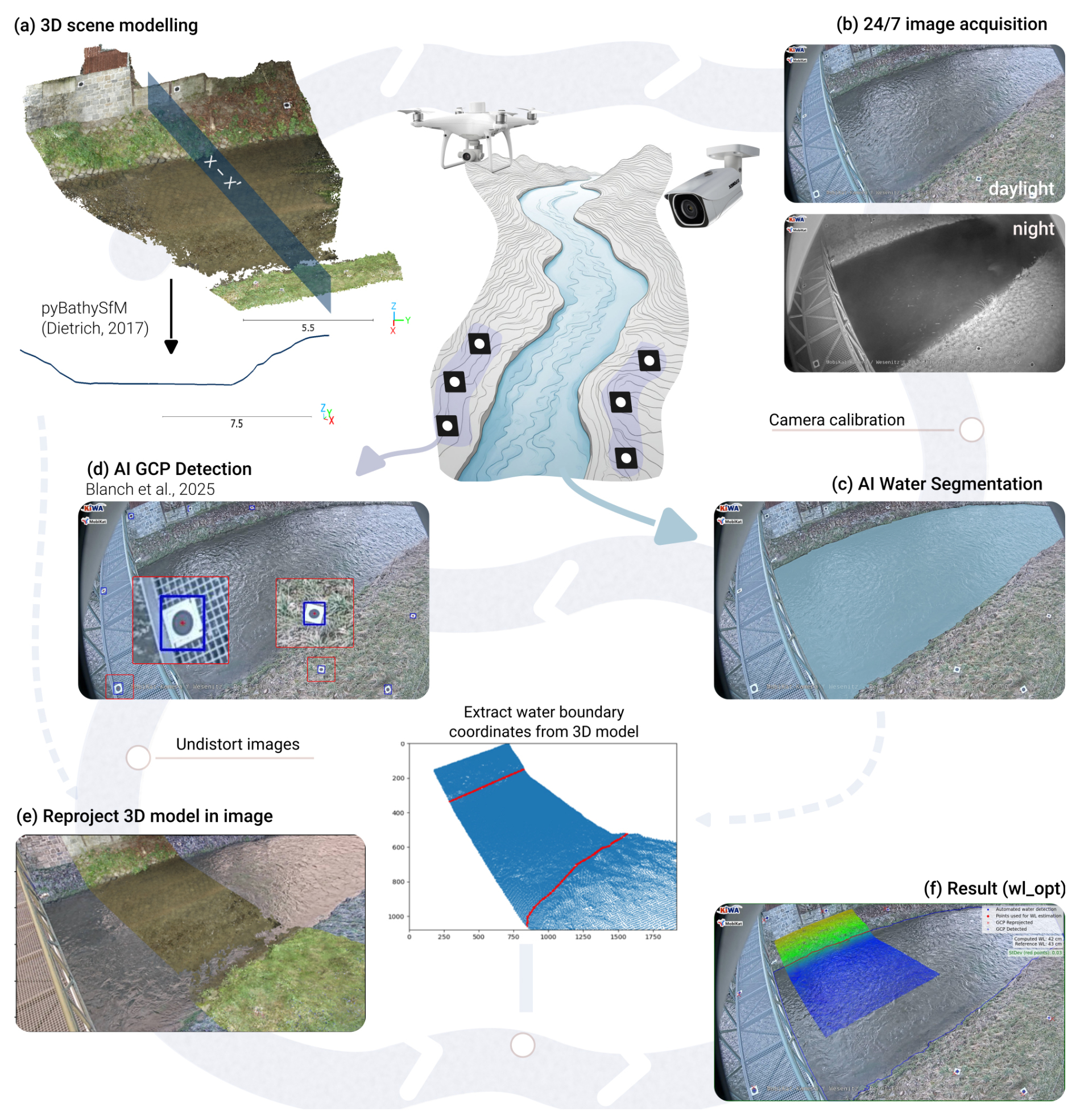
Figure 1 Graphical workflow for obtaining water level from an AI strategy for segmenting and identifying Ground Control Points (GCPs) and image-to-geometry for obtaining metric values of the water level.

2.1 Study area and data retrieval

The methodology was validated using images from four monitoring sites in Saxony, Germany, within the framework of the KIWA project (Grundmann et al., 2024). Three stations – Elbersdorf (ELB) on the Wesenitz River, Großschönau 2 (GRO) on the Mandau River, and Lauenstein 4 (LAU) on the Müglitz River – are co-located with official gauging stations operated by the Staatliche Betriebsgesellschaft für Umwelt und Landwirtschaft (the Saxon state company for environment and agriculture). The fourth site, Neukirch (NEU), is located on the Wesenitz River without a co-located gauge. At the three gauged sites, water level measurements derived from the camera system (wl_opt) are validated against official gauge records (wl_ref). These reference measurements are obtained by float-operated and bubble gauges (redundant measurement systems) and provide the most appropriate benchmark for operational validation because they represent independent, quality-controlled records reflecting accepted hydrometric practice (ISO 18365, 2013) and are used directly by flood services for decision-making. This comparison isolates the performance of the camera-based workflow from site-specific factors (e.g., camera placement, local calibration) and ensures the evaluation aligns with operational monitoring standards.

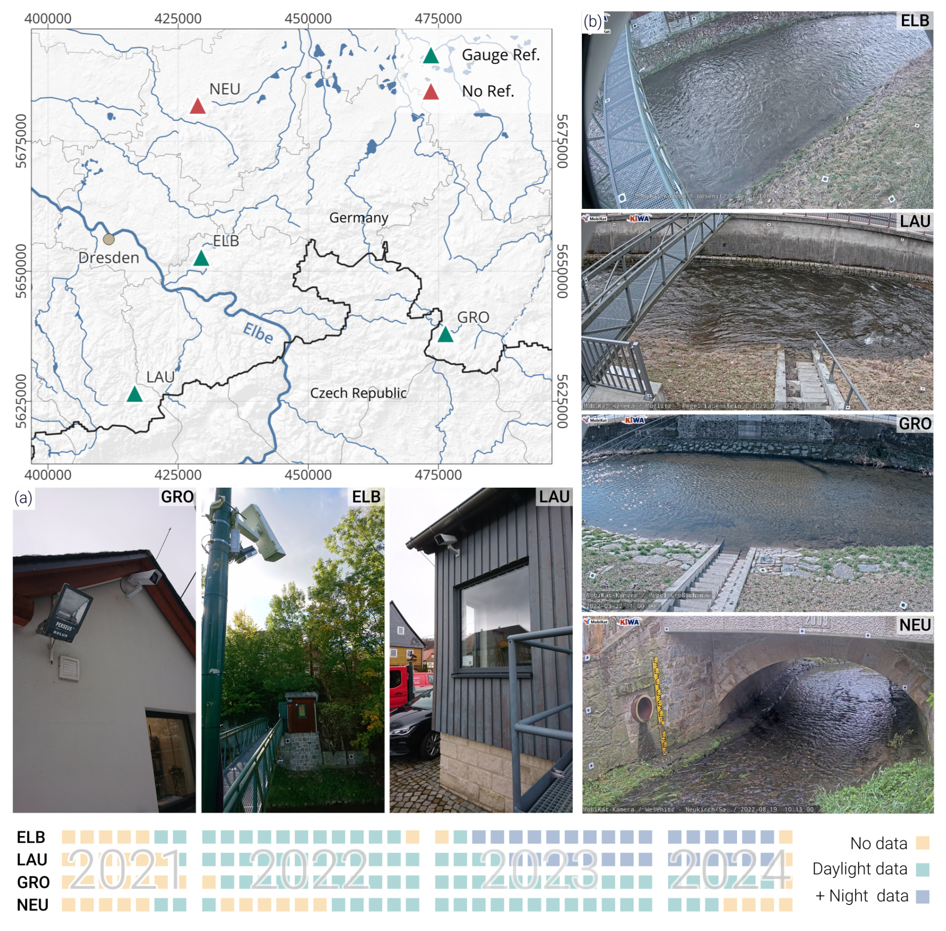
Figure 2 Geographic distribution and monitoring setup of study sites. Map indicates locations of GRO, ELB and LAU sites. Camera installations (a) and field views (b) at each site. Lower panel shows data acquisition periods.

Table 1 Image acquisition properties for each study area.

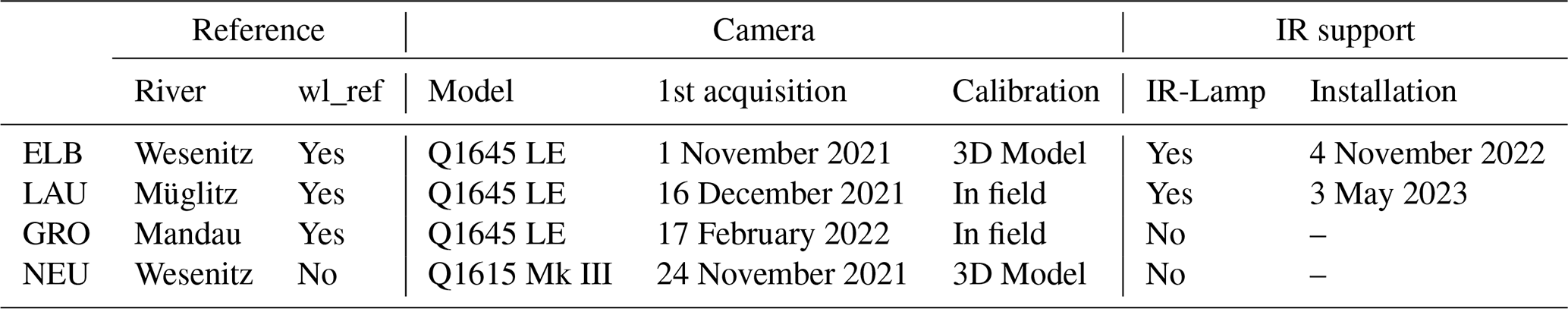
The images are captured using surveillance cameras, which provide an integrated solution for capturing images and videos and transmitting the data remotely to a server (Fig. 2a). Three stations (ELB, LAU, GRO) employ Axis Q1645 LE cameras (1920 × 1080 resolution, 3.75 µm pixel size), while NEU uses the Q1615 Mk III model (1920 × 1080 resolution, 2.90 µm pixel size) (Table 1). All cameras are equipped with zoom lenses (3–10 mm focal length) to optimize field-of-view coverage of the monitored river reach (Fig. 2b). Images are acquired at 15 min intervals (96 images per day) and transmitted automatically to a central server. Acquisition has operated continuously since late 2021, accumulating over 2.5 years of data through June 2024 (Table 1). To enable nighttime monitoring, remotely controlled infrared (IR) illumination was installed at ELB (November 2022) and LAU (May 2023), allowing 24 h observation. At GRO and NEU, nighttime images are captured but lack sufficient illumination for reliable water level estimation.

2.2 3D Modelling and Camera Calibration

Contactless water level measurement depends on establishing a metric reference frame that links 2D image pixels to 3D real-world coordinates. This is achieved through a georeferenced 3D model of the monitored river reach and ground control points (GCPs) visible in both the model and camera images. GCPs serve dual purposes: they enable photogrammetric determination of camera exterior orientation (position and viewing direction) and provide the geometric constraints necessary for an accurate 3D model registration. Proper spatial distribution of GCPs across the image frame ensures robust estimation of camera geometry. GCP coordinates were measured with centimeter accuracy using RTK-GNSS, and 3D models were generated using Structure-from-Motion Multi-View Stereo (SfM-MVS) photogrammetry from terrestrial and UAV imagery where feasible (e.g., Eltner and Sofia, 2020; Smith et al., 2016; Westoby et al., 2012), and the resulting model was georeferenced using both fixed and temporary GCPs measured with RTK-GNSS (Fig. 1a). Standard SfM-MVS reconstruction fails underwater due to refraction at the air-water interface. To address this, refraction correction was applied to submerged areas using PyBathySfM (Dietrich, 2017). When photogrammetric riverbed reconstruction was not feasible – due to high water levels or turbidity – cross-sections were surveyed with RTK-GNSS and interpolated to generate a riverbed mesh. Both approaches yield a gauge zero for the optical system (h_opt0), defined as the mean Z-coordinate of a central riverbed region (e.g., ELB: 4.5 m²). The gauge zero of the optical system (h_opt0) may differ from the gauge zero of the reference gauge data (h_ref0) due to differences in survey origin or riverbed morphology. To ensure direct comparability between datasets, we applied a bias correction to wl_opt by adding a constant offset. This offset was defined as the value that minimizes the mean residual between wl_opt and wl_ref, effectively removing the residual bias over the full observation period. The resulting offsets were small (ELB: −2.0 cm, LAU: −1.0 cm, GRO: −3.0 cm).

Photogrammetric image-to-geometry registration requires accurate interior camera parameters (focal length, principal point, distortion parameters). When feasible, cameras were calibrated before installation by capturing multi-perspective images of a coded calibration chart, with parameters estimated via bundle adjustment in Agisoft Metashape (v2.0.1) incorporating chart target coordinates (e.g., Liebold et al., 2023). When pre-installation calibration was not possible (cameras already mounted), interior parameters were estimated by incorporating fixed-camera images into the SfM bundle adjustment used for 3D modeling. Homologous points between mobile and fixed-camera images enabled parameter estimation, yielding an approximate calibration. LAU and GRO employed chart-based calibration; ELB and NEU required the SfM-based approach.

2.3 Image classification and filtering

Continuous 24/7 monitoring with surveillance cameras introduces the challenge of processing both daylight and low-light imagery, as cameras automatically switch to monochrome mode at night (Fig. 1b). To address this, images are classified based on RGB channel uniformity at diagnostic image locations: images with identical values across all three channels at all test pixels are classified as nocturnal. Without infrared (IR) illumination, nighttime images lack sufficient contrast for reliable river segmentation and are excluded from processing. At sites equipped with IR illumination (ELB, LAU), nighttime images are processed using night-specific segmentation parameters (Sect. 2.4). Daytime images undergo additional quality filtering based on sharpness. A Sobel edge-detection filter (threshold > 0.4) computes the mean edge strength across the image, enabling automatic exclusion of blurred, out-of-focus, or weather-obscured images (e.g., during heavy snowfall or fog). This filtering ensures that only images with sufficient clarity proceed to segmentation and photogrammetric processing.

2.4 AI Segmentation

Accurate water surface segmentation is fundamental to reliable automated water level estimation. Generic pretrained segmentation models (e.g., Segment Anything, SAM) lack the precision needed for reliable water level monitoring, (Zamboni et al., 2025), necessitating the development of domain-specific training. We employ a convolutional neural network (CNN) to segment water pixels from the background (Fig. 1c), based on the UPerNet architecture with a ResNeXt50 backbone (Xiao et al., 2018). This architecture was selected for its demonstrated performance on river segmentation tasks (Wagner et al., 2023).

The model was trained on the RIWA dataset (River Water Segmentation Dataset; Blanch et al., 2023b), which comprises 1163 manually labelled daylight images of water domains captured with diverse sensors (smartphones, drones, DSLR cameras), supplemented with images from WaterNet (Liang et al., 2020) and ADE20K images (Zhou et al., 2019). Part of the images used to create the RIWA dataset were also obtained with the KIWA project cameras (22 images, 1.9 % of the dataset).

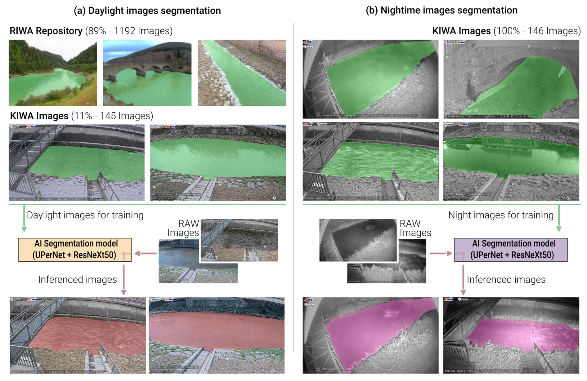
Figure 3 Data used for AI-based segmentation. Green areas represent manually segmented images, while orange/pink areas show the results obtained from the model for both (a) daytime and (b) nighttime images.

To optimize model performance, the original RIWA dataset was iteratively refined using Deep Active Learning (Li et al., 2024). This approach identifies images that are poorly segmented by the current model and prioritizes them for manual annotation and inclusion in subsequent training iterations. Through this process, challenging scenarios – such as adverse weather, transparent water, or strong shadows – were systematically incorporated into the training data. The final daytime dataset comprises 1,337 images, of which 145 (11 %) are KIWA images representing diverse locations, weather conditions, and water levels (Fig. 3a). For nighttime monitoring, a separate model – same network – was trained exclusively on infrared (IR) images. Due to the absence of publicly available IR river datasets, this training relied on 146 manually annotated KIWA IR images capturing varied weather and water level conditions (Fig. 3b). Both datasets are augmented using the Albumentation library (Buslaev et al., 2020), to increase training robustness and cross-site transferability. Augmentation is particularly critical for fixed-camera systems to prevent overfitting due to spatial correlations inherent in images from static viewpoints. Geometric transformations (rotation, scaling, flipping) were applied to break spatial dependencies, while pixel-level modifications (brightness, contrast, hue adjustments) were constrained to realistic ranges to preserve natural image appearance. Data augmentation was applied after generating all 512 × 512 patches from each original image in the training dataset, with each original patch producing four augmented versions. The UPerNet network with ResNeXt50 backbone was trained using the FocalLoss cost function and Adam optimizer (initial learning rate: 0.0001, reduced via ReduceLROnPlateau). Training was conducted on an NVIDIA GTX A6000 GPU with a batch size of 30 for 1000 epochs. Model performance was evaluated on an independent test set of 30 images, intentionally biased toward KIWA images (70 %) to prioritize optimization for operational monitoring conditions rather than generalized performance across all river imagery. The nighttime model was evaluated exclusively on KIWA images due to the lack of external IR datasets. The best-performing daytime model achieved 98.9 % pixel-wise accuracy, while the nighttime model reached 99.1 % accuracy, where accuracy represents the proportion of pixels correctly classified as water or non-water. Once trained, the models were deployed operationally to process incoming images every 15 min, automatically generating segmentation masks alongside each captured image (Fig. 3).

2.5 AI GCP Identification

Precise GCP coordinates in the acquired images are essential for an accurate image reprojection. Although cameras are mounted on fixed supports, thermal expansion, vibrations, and physical disturbances can cause subtle positional shifts that alter GCP image coordinates over time. Therefore, GCPs must be detected in every acquired image to maintain geometric consistency throughout the monitoring period (Fig. 1d). Automatic identification of GCPs in images is addressed differently in the literature, for example, using tracking algorithms (e.g., Eltner et al., 2017), feature descriptors like SIFT or SURF (Chureesampant and Susaki, 2014) or geometric shape-fitting (e.g., Maalek and Lichti, 2021). In this research, we employed an AI-based approach using an adapted R-CNN Keypoint detector neural network, specifically retrained on KIWA imagery to identify GCP centers directly. This method, detailed in Blanch et al. (2025a) achieves sub-pixel precision (< 0.5 pixel) without requiring pre- or post-processing and demonstrates robust performance under conditions where traditional feature-based methods fail (e.g., varying illumination, partial occlusions, weathering; Blanch et al., 2025a). When the detector fails to identify one to four GCPs – due to temporary occlusion, extreme weather, or imaging artifacts – missing coordinates are estimated using the KNNImputer algorithm (scikit-learn). This approach leverages temporal coherence by identifying recent images with similar GCP configurations and interpolating missing values from their coordinates. If more than four GCPs cannot be detected, coordinates from the most recent valid image are assigned. This fallback strategy maintains operational continuity while flagging potentially degraded measurements for quality assessment.

2.6 Photogrammetric process

The photogrammetric process transforms the AI-segmented water boundary from image space to real-world coordinates by establishing the geometric relationship between the 2D image plane and the 3D site model (see Elias et al., 2019; Eltner et al., 2018 for detailed explanation) (Fig. 1e). Exterior orientation parameters – defining camera location and rotation – are computed by solving the collinearity equations that relate the detected 2D GCP coordinates to their known 3D world coordinates. This geometric solution enables reprojection of the 3D point cloud onto the image plane, where each pixel can be assigned its corresponding real-world 3D coordinate. To extract water level from the segmented image, the upper contour of the water mask (the river edge opposite to the camera) is intersected with the reprojected point cloud using nearest-neighbour search. The search is spatially constrained to a central cropped region of the point cloud, ensuring that only reliable portions of the 3D model contribute to the measurement.

Water level is derived from the statistical distribution of Z coordinates along the extracted water-edge points. The median Z value represents the water surface elevation (h_opt), which is then converted to water level by referencing to a baseline elevation (Eq. 1):

$$\begin{array}{}\text{(1)}& \mathrm{wl}\mathit{\_}\mathrm{opt}=h\mathit{\_}\mathrm{opt}-h\mathit{\_}\mathrm{opt}\mathrm{0}+\mathrm{offset}\end{array}$$

The standard deviation of Z coordinates along the intersected points serves as a quality indicator, with higher dispersion suggesting segmentation uncertainty or non-horizontal water behaviour. Validation of the proposed method is conducted at three sites equipped with official gauging stations (ELB, LAU, and GRO), where wl_opt measurements are benchmarked against reference values (wl_ref). Reference measurements represent 15 min averages computed from 5 min sampling intervals, whereas wl_opt values correspond to instantaneous observations. To account for this temporal mismatch and reduce the influence of short-term fluctuations, accuracy assessment is performed using daily-averaged values for both wl_opt and wl_ref. Because the workflow operates fully autonomously on all acquired images, automated quality control is essential to identify and filter erroneous measurements. Two statistical criteria are applied. First, measurements with excessive standard deviation in the Z coordinates of water-edge points are rejected, as high dispersion indicates that the segmentation boundary intersects multiple elevation levels – inconsistent with the expected horizontal water surface. Second, extreme outliers in wl_opt relative to wl_ref are identified using a modified Tukey filter with twice the interquartile range (2 × IQR), removing measurements that deviate significantly from the expected temporal behaviour.

3 Results

Data from the operational automated camera monitoring system between late 2021 to June 2024 was used, with observation periods ranging from 660 d at NEU to 864 d at GRO and 917 and 927 d at ELB and LAU, respectively (Table 2). Over these periods, the cameras acquired 33 382 images at NEU, 47 109 at GRO, 71 787 at ELB and 65 631 at LAU, providing between 660 and 927 d of 15 min (96 images per day) water level observations at the four stations (Table 2). Except for ELB, where technical issues caused data gaps, image acquisition was continuous throughout the observation periods at all locations (Table 2). Quality filtering via Sobel edge detection removed only a small fraction of the acquired images, with rejection rates below 1 % at ELB and LAU and values of 1.2 % and 9.6 % at GRO and NEU, respectively (Table 2). These rejected images are mainly affected by adverse weather conditions such as fog or heavy snowfall, or by low light levels around sunrise and sunset; in addition, high ambient light in the urban environments of NEU and GRO occasionally triggered the surveillance cameras to remain in day mode during the night, producing low-contrast images that failed the Sobel criterion and explaining the higher rejection rates at these sites (Table 2). Among the images passing the Sobel filter, the AI workflow successfully delivered a result for 99.3 %–100 % of the inputs at all stations, after which the standard-deviation filter rejected between 0.1 % and 3.8 % of these results depending on the site (Table 2). At the three gauged stations (ELB, LAU and GRO), the final Tukey outlier filter based on 2 × IQR further removed only 1.2 %–2.6 % of the standard-deviation-accepted measurements (Table 2). The measurements that remain after this Tukey filtering step define the final validation dataset used to compute the water-level error metrics reported in the following subsections. Relative to all acquired images, the overall proportion of valid water-level estimates ranges from 86.9 % at NEU, where a fraction of the images was incorrectly acquired due to urban lights, to 98.1 % at LAU, with 95.3 % and 97.1 % of the images yielding a valid water level at GRO and ELB, respectively (Table 2).

Table 2 Image acquisition, filtering and processing statistics at each monitoring station, summarising the number of acquired images, the fractions removed by filters, and the resulting proportion of valid water-level measurements. No Tukey filter is applied at NEU due to the absence of a reference gauge at this site.

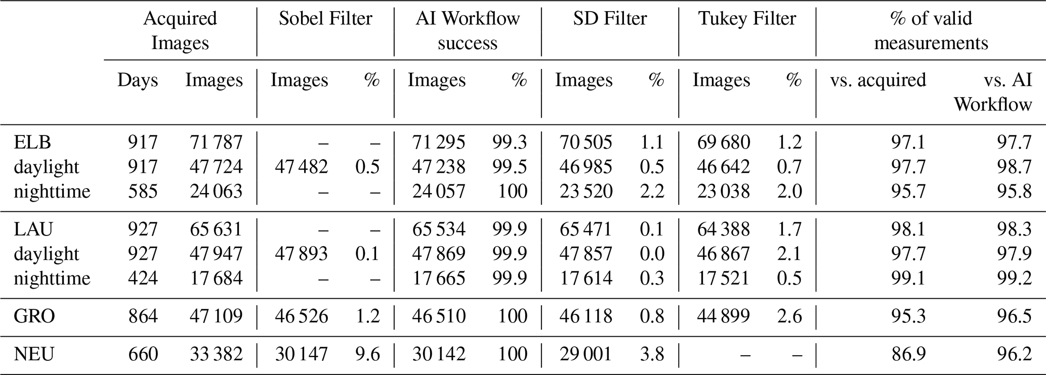
Table 3 Camera focal length and reprojection error of ground control points (in pixels) at the four monitoring stations.

Geometric accuracy of the image-to-geometry registration was assessed using the reprojection errors of the ground control points (GCPs) at each station (Table 3). Average reprojection errors range from 4.9 pixels at NEU and 6.3 pixels at LAU to 17.5 pixels at ELB and 29.0 pixels at GRO. The lower mean errors at LAU and NEU reflect the dedicated calibration-camera setups used at these sites, whereas the higher values at ELB and especially at GRO indicate a more challenging imaging geometry and stronger lens distortions. In all cases, the GCPs were deliberately positioned near the image edges, where distortions are most pronounced, so the reported values represent a conservative estimate of the registration quality between the 3D model and the 2D camera images.

Table 4 Statistical comparison between wl_opt and wl_ref over the entire observation period, for individual measurements and daily averaged values.

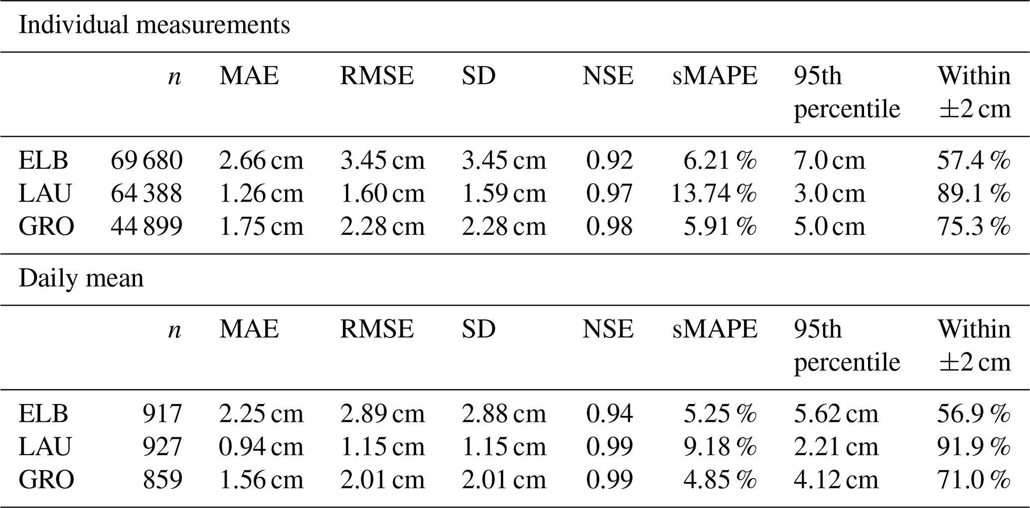
Table 4 reports the error statistics between the camera-based water levels (wl_opt) and the gauge records (wl_ref) for the three gauged stations, considering both all individual results and daily averaged values. For individual estimates, mean absolute errors (MAE) are in the centimetre range at all sites, from 1.26 cm at LAU to 2.66 cm at ELB, with GRO in between. With respect to the ±2 cm accuracy threshold commonly used in German guidelines for operational water-level monitoring (LAWA, 2018), between 57.4 % (ELB) and 89.1 % (LAU) of the measurements fall within ±2 cm of the reference, and 75.3 % of the measurements at GRO satisfy this criterion. The 95th percentile of the absolute differences ranges from 3.0 cm at LAU to 7.0 cm at ELB, showing that large discrepancies are infrequent and that, at the best-performing sites, most errors are limited to a few centimetres.

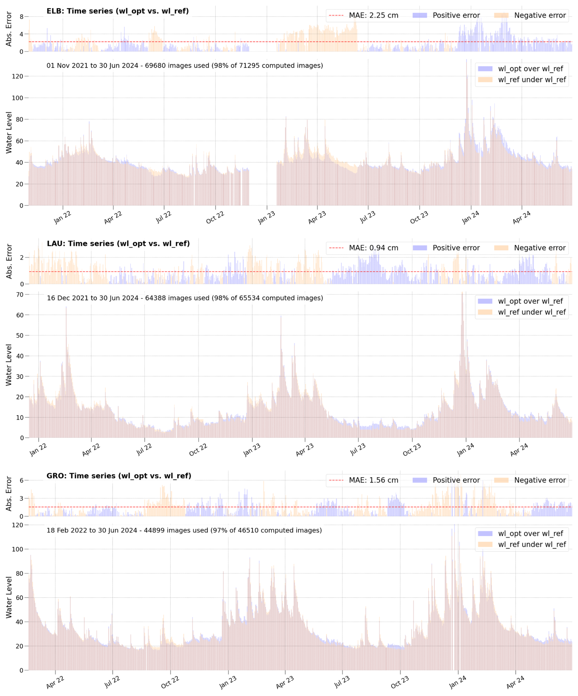
Figure 4 Multi-site water level time series validation. Absolute error time series (top panels) and daily mean water level time series (bottom panels) comparing wl_opt and wl_ref at ELB, LAU and GRO sites. Shaded areas indicate periods where wl_opt exceeds wl_ref (blue) and where wl_ref exceeds wl_opt (orange).

The error statistics reported in Table 4 are consistent with the patterns shown in Fig. 4, which presents time series comparisons of wl_opt and wl_ref at the ELB, LAU, and GRO monitoring sites for the complete observation periods. For each site, the upper subplot displays the absolute differences as time series. The main subplot presents the time series of daily averaged water levels from both measurements, showing that wl_opt closely tracks wl_ref across a wide range of conditions, including both low-flow and high-flow events, with only centimetric deviations overall. While the largest departures from the reference typically occur during rapid level rises – such as the January 2024 events (4 cm at LAU for water levels near 70 cm, 8 cm at ELB above 150 cm, and 7 cm at GRO above 120 cm). These deviations can be attributed to differences between the measurement concepts, as the reference gauges provide 15 min water levels averaged over 5 min sampling intervals, which tend to smooth rapid fluctuations typical of flood events, whereas the camera-based estimates are derived from instantaneous images.

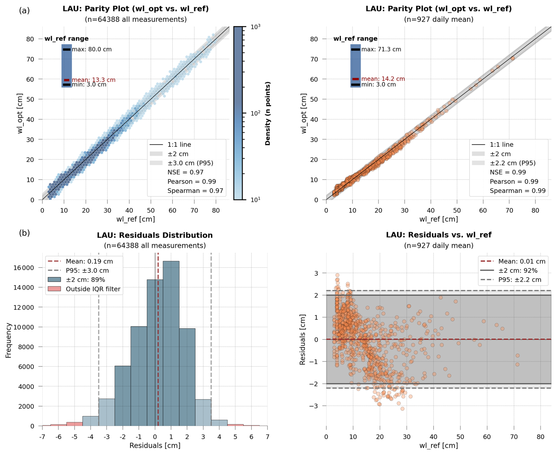
Figure 5 Validation metrics for LAU monitoring site. (a) Parity plots for all measurements (top left) and daily means (top right, scatter). (b) Bottom panels show detailed residuals analysis for all measurements: distribution histogram (left) and scatter plot vs. water level (right) for daily mean values.

Figure 5 presents the statistical validation for LAU. The parity plots (Fig. 5a) show a close agreement between wl_opt and wl_ref over the full range of observed water levels (3–80 cm), with Pearson = 0.99 and Spearman = 0.97. To keep the comparison legible given the large sample size (n = 64 388), all individual measurements are represented as a hexbin density map, whereas daily means (n = 927) are plotted as individual points, both clustering around the 1 : 1 line. Nash–Sutcliffe efficiency values are also high at all sites, ranging from 0.94 to 0.99 (Table 4). The residuals analysis (Fig. 5b) indicates that 89 % of measurements fall within ±2 cm and that the 95th percentile is ±3.0 cm. A slight systematic pattern is observed, with residuals tending to increase with water level, particularly between 15–30 cm, which may be related to the presence of a step in the measurement wall at LAU. Summary statistics for the three monitoring sites are reported in Table 4, and the corresponding parity and residual plots for ELB and GRO are provided in Appendix C (Figs. C1 and C2, respectively).

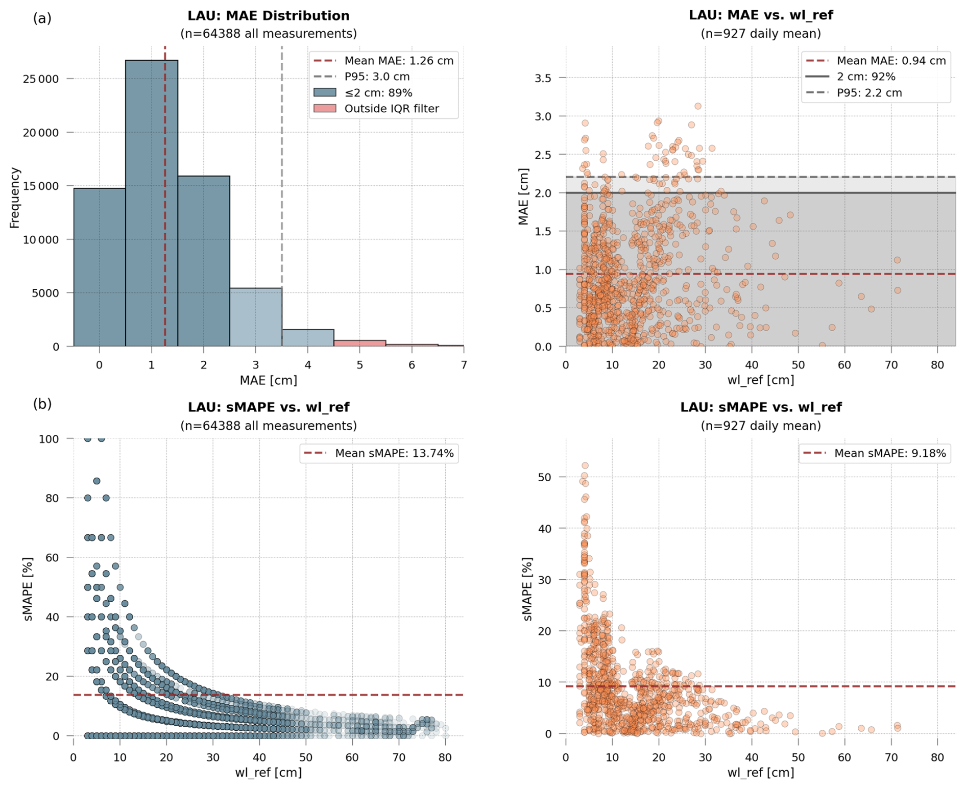
Figure 6 Error metrics for LAU monitoring site. (a) MAE distribution (top left) and MAE vs. water level (top right) for all measurements and daily means. (b) sMAPE vs. water level (bottom) for all measurements (left) and daily means (right).

Figure 6a summarises the distribution of absolute errors at LAU, both for all measurements and for daily means, including the 95th percentile and the fraction of values within ±2 cm; equivalent MAE plots for ELB and GRO are provided in Appendix C (Figs. C3a and C4a). When the data are aggregated to daily means, the temporal mismatch between instantaneous wl_opt and averaged wl_ref is partly smoothed and the errors decrease further. Daily MAE is 0.94 cm at LAU and remains below 2.25 and 1.56 cm at ELB and GRO, respectively, while the 95th percentile of the daily absolute differences ranges from 2.21 cm at LAU to 5.62 cm at ELB. At LAU, in particular, 95 % of the daily mean values differ from the gauge record by less than about 2.2 cm and 91.9 % of the days remain within ±2 cm of the reference, indicating that most daily water levels derived from the optical method deviate from the gauge by only a few centimetres. Figure 6b shows the corresponding symmetric mean absolute percentage errors (sMAPE) at LAU for all measurements and for daily means, while the analogous plots for ELB and GRO are again presented in Appendix C (Figs. C3b and C4b). For daily averaged water levels, sMAPE values remain around 5 % at ELB and GRO, whereas values close to 9 % at LAU mainly reflect centimetric fluctuations over very low water levels, where small absolute differences translate into comparatively large relative errors. This behaviour is consistent with the sMAPE–wl_ref relationships, which show decreasing relative errors as water levels increase at the three monitoring sites.

Table 5 Statistical comparison between wl_opt and wl_ref for the first 180 d of operation at each station, for individual measurements and daily averaged values.

To assess temporal stability and the need for maintenance, the same statistics were computed for the first 180 d of operation at each station (Table 5). For ELB and GRO, all key metrics improve in this initial period compared to the full time series, with lower MAE and 95th percentiles and a higher fraction of daily values within ±2 cm of the reference. At LAU, the performance during the first 180 d is very similar to that of the complete period: individual MAE and the 95th percentile remain essentially unchanged, and daily MAE and the fraction within ±2 cm are only slightly less favourable, indicating that the system maintains a stable accuracy over time.

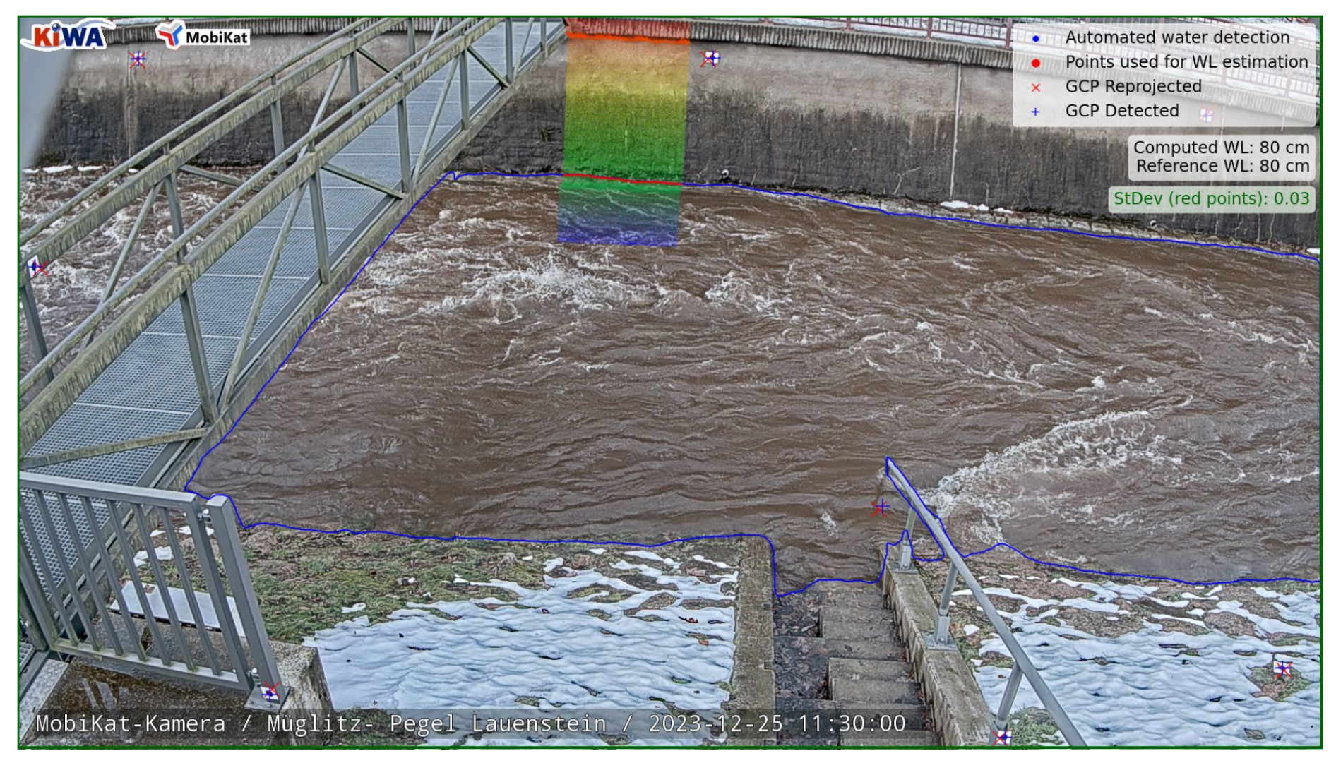
Figure 7 Automated water-level measurement at peak-flow conditions at LAU (December 2023). The image shows the detected ground control points (crosses), the segmented water-surface boundary (blue line), the upper contour segment used for water-level estimation (red line), and the section of the 3D model colored according to the Z coordinate.

Figure 7 shows the measurement computed at the time of the maximum water level at the LAU station. The figure includes the original image captured by the cameras, the re-projection of the 3D model used to calculate the Z coordinate, the automatically detected GCPs (crosses), the segmented water boundary (blue line), and the specific water-surface segment used to extract the Z coordinate (red points), together with the comparison between wl_opt and wl_ref at the stations where a gauge is available (ELB, LAU and GRO). A video animation illustrating the water-level measurements obtained at the LAU gauging station between 24 and 31 December 2023 is provided in Blanch et al. (2025b) and referenced in the Video Supplement section. Similar peak-flow visualisations for the ELB and GRO stations are presented in Figs. C5 and C6, respectively, in the Appendix.

4 Discussion

The main contribution of this work is the demonstration of a robust solution for water level measurement using low-cost and contactless methods. The systems were tested over 2.5 years at four study sites in Saxony, Germany. The addition of IR lamps has addressed one of the primary limitations of visual methods, enabling reliable measurements at night and allowing for continuous 24 h monitoring. By integrating AI into the photogrammetric workflow, the system proves to be highly robust, functioning effectively also under adverse weather conditions (Fig. 8). The utilization rate of images is very high (average of 98 %), indicating that the system rarely fails to resolve a valid water level. Failures typically occur during periods of extremely poor visibility (e.g., fog, heavy snowfall), when the image-based method is not viable due to inadequate observation of the water surface (Fig. 9a and b).

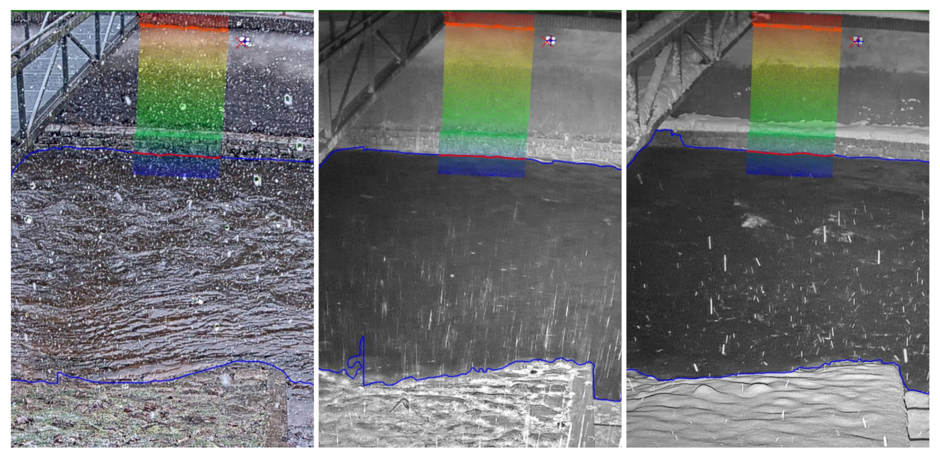
Figure 8 Successful water level measurements at LAU during snowfall events of varying intensity, showing robust AI segmentation and GCP identification under adverse weather conditions.

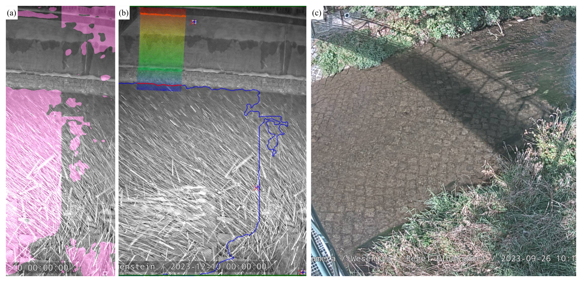
Figure 9 Main limitations of the automated camera gauge system. (a, b) LAU during intense snowfall: (a) erroneous AI segmentation due to poor visibility, and (b) same image that despite segmentation errors, a valid water level measurement was obtained. (c) ELB with excessive vegetation covering both riverbanks, obscuring most ground control points and preventing clear water-slope contact delineation.

The success in obtaining water level values under adverse weather conditions is due to our iterative training process of the neural network for water segmentation in images. We developed a model that can handle a wide variety of situations effectively including images that the AI initially struggled to resolve in successive training sessions. It should be noted that KIWA images constitute less than 11 % of the training dataset, suggesting the model's high transferability. For future installations with different cameras and environments, only a small number of manually labelled images will be needed to adapt the model to the new site, because the bulk of the training data come from the RIWA dataset, which spans highly diverse aquatic domains (rivers, lakes, seas, urban environments, etc.). Adding a small percentage of site-specific images ensures maximum segmentation accuracy and, crucially, enables evaluation on the actual target domain, yielding a model tailored to the study area rather than a generalised classifier trained on unrelated scenes (e.g. coastal imagery). Furthermore, modern fine-tuning techniques that retrain only the final network layers can reduce deployment effort even further, potentially avoiding full retraining altogether. This transferability has been successfully demonstrated in practice by Krüger et al. (2024), where the workflow was retrained and applied in a very different environment in Oman, yet still delivered robust results.

The segmentation of images for precise water level measurement presents a significant challenge (i.e., Moghimi et al., 2024; Wagner et al., 2023) because it requires precise identification of the interface between the water body and the riverbanks in the image. This boundary is especially difficult to detect accurately in automatic segmentation processes, since on the one hand it is a natural boundary (i.e., waves, water transparency, vegetation), and on the other hand standard metrics such as the Intersection over the Union (IoU) or the Dice coefficient, and therefore the most common models, give priority to the precise segmentation of the whole object rather than to the precise definition of the contour. In a river context, this delineation is especially challenging due to water transparency at the boundaries, which makes clear delimitation difficult even for human observers. Although we did not employ a contour-centred metric such as the Boundary F1 Score (BFScore), testing various neural network models (Wagner et al., 2023) has allowed us to identify the optimum for correct water segmentation, and thus obtain water level measurements.

Training with night time images proves to be more feasible and accurate because the contrast between the water and the background is more pronounced. Additionally, there are no transparency issues due to the high absorption of infrared light by water, which simplifies the segmentation process. The precision obtained during training for the best-performing model (around 99 %) is consistent with the model's performance throughout the entire time series, demonstrating its ability to consistently segment the water bodies in most images. Ensuring that the mask intersecting with the 3D model accurately represents the water boundary at the moment of image acquisition. The results obtained are in line with the ones provided by Wagner et al. (2023) and Moghimi et al. (2024) in their respective research. However, generalising the use of near-infrared imagery to daytime conditions instead of RGB – with the aim of simplifying segmentation – is not fully reliable. Daylight IR-only thresholding is unreliable because solar NIR and sunlight vary with illumination geometry and surface reflections, which can reduce image sharpness and detail, whereas the nighttime approach operates under controlled illumination and yields more stable contrast.

The automatic identification of GCPs in each image prevents the accuracy from deteriorating over the observation period as effects by experienced camera movements, e.g. due to thermal effects on the camera (Elias et al., 2020), are mitigated. The main issue with the use of GCPs has been their durability in the study areas. Although most remained throughout the 2.5-year study, some were damaged or displaced during high-flow periods or shaded temporally due to vegetation cover, indicating that even with an automated camera gauge, maintenance is necessary. Regarding this maintenance, the difference between Table 4 (whole time series) and Table 5 (first 6 months) shows how the error between the optical values and the reference is higher the longer the time window, and although this difference is multifactorial, undoubtedly the deterioration of the GCPs as well as the age of the camera calibration play an important role. Also, maintenance is necessary due to other key factors such as vegetation. Our results indicate that vegetation significantly impacts deviations to the references by either obscuring GCPs or covering the water-shore contact, leading to irregular segmentation. An effective solution involves automatic regeneration of the 3D models updating the model to the real riverbank situation; however, a crucial aspect of ensuring the robustness of the method is to use measurement areas where the water-slope contact remains unobstructed over time. Figure 4 illustrates how, particularly during summer, sudden changes lead to the system underestimating or overestimating values (notably in ELB, July 2023). These anomalies are related to vegetation changes, with abrupt shifts corresponding to days when landscaping work was performed. Conversely, stations like LAU show more stable values and lower absolute error throughout the year, as the water-shore contact occurs on a concrete wall, providing greater stability over time.

In addition to the accurate segmentation of water and the identification of GCPs, another crucial element for ensuring good water level measurement is the proper calibration of the fixed cameras. This was challenging if the cameras were already installed and operational. In our case, we observe that the ELB camera, which was already in operation and calibrated approximately (i.e., adding the image into the SfM bundle adjustment), shows slightly different precision compared to LAU, where a much more precise calibration was performed (i.e., field board calibration). GRO also underwent field calibration, but the use of a very short focal length and the large distance of the ROI to the camera adversely affects precision. During the two years, the camera calibration files had not been modified. However, assuming a temporal stable interior camera geometry is unlikely amongst other due to the influence of temperature changes (Elias et al., 2020). In the future, refining the results will require the ability to self-calibrate the camera (i.e., obtaining internal parameters) on-site during the analysis of each image (e.g., as done and assessed in Elias et al., 2023).

Table 3 illustrates how cameras with shorter focal lengths exhibit greater re-projection errors. This is expected, as they tend to have higher distortions, particularly at the edges of the image where the GCPs are located. Nevertheless, the results demonstrate that the photogrammetric approach and calibration methods worked sufficiently. Notably, the case of NEU is significant, where despite not having undergone field calibration, the re-projection values are comparable to those obtained at LAU. The acquisition of GCP coordinates and camera calibration are crucial for achieving accurate exterior camera parameter estimation. Errors at these steps affect the accuracy of the reprojection of the 3D model into the 2D space and the subsequent extraction of the Z coordinates.

The creation of the 3D model using SfM algorithms proved to be effective, particularly during normal and high water levels. In urban areas (e.g. GRO and NEU) the models are created using terrestrial cameras only, while at other study sites UAV images are combined. In both cases, the riverbed has to be corrected for refraction influences. In GRO, a larger offset (i.e., −2.5 cm) has to be applied to the wl_opt to minimise the discrepancy between the references zero heights due to the difficulties in accurately modelling the riverbed due to significantly higher water levels on the day of image acquisition. For deep rivers, where SfM cannot be applied because the riverbed is obscured, GNSS support for tracing cross-sections is necessary. In general, a change in absolute error has been observed when the calculated water level intersects the area of the model that is underwater, as the reconstruction quality of this zone is lower. Although this is not a critical issue, if the camera system is used for measuring higher water levels (e.g. floods). Here, we suggest that the 3D model should be generated during periods of lower water levels to improve the accuracies.

The intersection of the water body boundaries with the 3D model determines the calculated water level, making precision in both elements crucial. The standard deviation of the extracted Z coordinates provides an indication of the quality of the intersection, as we assume that the intersection should occur at a constant elevation (i.e., the same Z coordinate). Measurements with high standard deviation suggest difficulty in estimating a stable Z value, which typically indicates either an erroneous segmentation of the water pixels or that the water body-shore contact is not clearly visible in the image (e.g., vegetation obscuring the contact, Fig. 9c). However, the percentage of results filtered by standard deviation (Table 2) is not high, demonstrating the robustness of the method. The application of the Tukey filter based on official reference values has minimal impact on the total number of images used and is only applied to remove erroneous values that may have passed through the standard deviation filter. Typically, these errors are sporadic and also relate to poor segmentation (i.e., segmentation is performed in tiles that may produce horizontal lines intersecting constant Z values), poor image visibility (e.g., presence of ice or animals on the camera), or a water level too low leading to intersections with the 3D model in areas where reconstruction was not optimal.

Regarding the results obtained, the three stations show distinct performance patterns that can be directly related to their installation conditions. At LAU, the precision is consistently high over more than two years, with a daily mean MAE of 0.94 cm and an individual-measurement MAE of 1.26 cm (Table 4). The distribution of individual errors is also compact, with a 95th percentile of 3.0 cm, indicating that most image-based water levels remain very close to the reference even in the upper tail of the error distribution. This behaviour confirms the configuration at LAU as a best-case scenario for future installations: the camera was calibrated on-site, a moderately large focal length was selected to reduce distortions, and the water–shore contact occurs on a concrete wall without vegetation at a moderate distance from the camera, which simplifies segmentation and stabilises the geometry. In contrast, the ELB study site exhibits higher and more variable errors. Over 917 d of monitoring, the daily mean MAE is 2.25 cm and the individual-measurement MAE reaches 2.66 cm, while the 95th percentile of individual errors rises to 7.0 cm (Table 4). These larger deviations are consistent with the challenging water–shore interface at ELB: the contact zone is frequently obscured by vegetation, and the segmentation of the waterline is therefore less stable. Figure 4 – ELB, clearly shows abrupt changes in wl_opt, especially during summer, which coincide with vegetation maintenance and highlight the influence of local riverbank dynamics. Similar vegetation-related issues have been reported in previous image-based water level studies by Eltner et al. (2018) and Peña-Haro et al. (2021). In addition, the presence of a small hydroelectric power plant 100 m upstream introduces rapid changes in water level on the order of decimetres within a few minutes, while the official gauge provides 15 min averages. During such events, the averaged reference value may not represent the instantaneous water level seen by the camera, adding background noise to the error statistics. GRO occupies an intermediate position between LAU and ELB. Here, the daily mean MAE is 1.56 cm and the individual-measurement MAE is 1.75 cm, and the 95th percentile of individual errors reaches 5.0 cm (Table 4). Although the camera was calibrated in the field, the width of the river, the 20 m distance between the camera and the waterline, the use of a wide-angle lens and the partial loss of GCPs increase the sensitivity of the 3D reconstruction and camera orientation to small geometric errors. In addition, the quality of the water–shore contact varies with water level: at higher stages the contact occurs against vertical or near-vertical walls that are easy to delineate, whereas at lower stages it shifts onto a sloping bank with rocks and vegetation, making segmentation more difficult in a way that is similar to ELB. These factors explain why GRO performs clearly better than ELB but does not reach the stability observed at LAU.

During the first 180 d of operation (Table 5), the three stations exhibit very similar behaviour: individual-measurement MAE values range between 1.24 and 1.78 cm, and the 95th percentiles vary between 3.0 and 5.0 cm. For daily means, MAE values are around 0.8–1.6 cm over this initial period. This phase can be regarded as a benchmark for a newly implemented low-cost camera system under favourable and well-maintained conditions, when GCPs are intact, vegetation has limited impact and the camera calibration is recent. When extending the analysis to the full observation period, the degradation of performance at ELB and, to a lesser extent, at GRO becomes apparent (Table 4). The increase in MAE and in the 95th percentiles is consistent with progressive GCP damage or loss, vegetation growth in the water–shore contact zone and ageing camera calibration. In LAU, the daily mean MAE over the whole period is slightly lower than during the first 180 d because the offset used to minimise the differences with the reference is estimated over the entire time series, which partially compensates for initial biases. However, the individual-measurement statistics at LAU still reflect the long-term stability of this installation. Overall, these patterns indicate that camera-based gauges can maintain high accuracy over several years, but only if supported by periodic maintenance and occasional updates of the 3D model and camera calibration.

When comparing our results to previous work conducted at the same study sites, several key differences emerge in terms of precision, operational robustness, and temporal coverage. Eltner et al. (2021) reported an error of −1.1 ± 3.1 cm at ELB using smoothing algorithms, with a best Spearman coefficient of 0.93, but noted significant seasonal variability that affected measurement consistency. Zamboni et al. (2025) proposed a computationally efficient method avoiding model training, achieving mean absolute errors of 2.1 cm (LAU) and 2.9 cm (ELB) with RMSE values ranging from 1.6 to 3.2 cm across their three camera-gauge stations (Wesenitz, Elbersdorf, Lauenstein). While both studies demonstrate valuable methodological contributions, neither addressed night-time observations, long-term resilience to adverse weather conditions, or extended time-series stability. Our approach builds upon this foundation by maintaining comparable or improved precision while systematically evaluating performance over multi-year deployments under full operational conditions at these same locations, including challenging scenarios that previous work did not consider.

Compared to other image-based contactless systems deployed at different sites, our results achieve precision levels competitive with existing methods while extending the evaluation to multi-year continuous operation under full 24/7 conditions, including nighttime and adverse weather. Short-term experimental studies typically cover periods from hours to weeks: Erfani et al. (2023) obtained RMSE values between 1.5 and 2.9 cm over a few hours at Rocky Branch (South Carolina), Muhadi et al. (2021) achieved Spearman correlations of 0.91 using DeepLabv3 in Malaysia, Wang et al. (2024) obtained 0.87–0.94 over two weeks in UK rivers, and Moy de Vitry et al. (2019) reached 0.75–0.85 with U-Net on Swiss CCTV footage using the SOFI trend index. Among longer-term deployments, Vandaele et al. (2021) reported Pearson correlations of 0.94–0.96 over one year using landmark-based water level estimation on UK rivers, while LSPIV-based systems have demonstrated extended capabilities: Ran et al. (2016) obtained RMSE of 3.7 cm over flood events in a Chinese mountainous stream, Stumpf et al. (2016) achieved MAPE of 9 % over 2.5 years analyzing more than 4000 videos in a tropical mountain river (Réunion Island), and Peña-Haro et al. (2021) reported RMSE of 6.8 cm across multiple Swiss Alpine sites with their operational DischargeKeeper system. Our work bridges the gap between experimental validation and operational deployment, achieving Spearman correlations of 0.94–0.97 and Pearson correlations of 0.97–0.99 over multi-year continuous monitoring that consistently captures different hydrological regimes and challenging environmental conditions – a combination of accuracy, duration, and robustness not previously demonstrated in camera-based systems.

The results of this study are consistent with the German manual for river water level measurements, requiring water levels with accuracies below 2.0 cm as an acceptable systematic error (LAWA, 2018). When considering the entire observation period (Table 4), both LAU and GRO still maintain a high proportion of daily means within ±2 cm of the reference (91.9 % and 71.0 %, respectively), confirming that the camera-based gauges can meet hydrometric standards over multi-year deployments. In contrast, ELB clearly performs worse in this respect, with only 56.9 % of daily means within the 2 cm range, which is consistent with the site-specific issues at this station already discussed. Nevertheless, during the first 6 months of operation all three stations showed substantially higher fractions of individual measurements within ±2 cm (Table 5), indicating that under favourable and well-maintained conditions the system can achieve very similar performance across different sites. However, the error levels observed here are consistently lower than those relevant for flood detection and AI-based observation, making our approach suitable and advantageous for continuous river monitoring and early warning systems. In addition, the stability achieved in the water level estimates provides a solid basis for further developments in river monitoring through camera-based gauges and video series, enabling future integration of image-based methods to derive flow and velocity.

5 Conclusion

This study demonstrates the effectiveness of an AI-enhanced, image-based camera gauge for long-term, near real-time river water level monitoring. Over a 2.5-year period, the system delivered accurate water level estimates at three contrasting sites, with daily mean MAE values as low as 0.94 cm and individual-measurement MAE values between 1.26 and 2.66 cm, which are consistent with, and in most cases comfortably below, the 2.0 cm accuracy requirement of the German manual for river water level measurements. The combination of neural networks for water segmentation and GCP identification with a photogrammetric workflow enabled fully automatic processing of large image datasets under a wide range of hydrological and environmental conditions. The approach relies on low-cost hardware and standard surveillance cameras, which facilitates deployment at additional sites and integration into existing hydrometric networks. The installation of IR lamps, combined with the surveillance cameras' ability to capture nighttime images, mitigated one of the major limitations of image-based methods, namely their restriction to daylight, and enabled continuous 24/7 water level monitoring, which is particularly relevant for flood early-warning applications. The observed increase in inaccuracies over time highlights the need for proper maintenance of both the environment (e.g. vegetation) and the cameras (e.g. calibration). Future work aimed at minimising these maintenance requirements, for example by regenerating 3D models to adapt to terrain changes and by implementing automatic camera calibration procedures, is expected to further improve measurement quality and robustness.

Appendix A

A1 Nomenclature and Abbreviations

ADE20K	Semantic scene dataset used for segmentation benchmarks
AI	Artificial Intelligence
BFScore	Boundary F1 Score
CNN	Convolutional Neural Network
DSLR	Digital Single-Lens Reflex
GCP	Ground Control Point
GNSS	Global Navigation Satellite System
IoU	Intersection over Union
IQR	Interquartile Range (Q3–Q1)
IR	Infrared
KNNImputer	k-Nearest Neighbours Imputer algorithm (scikit-learn)
LBWLE	Landmark-Based Water Level Estimation
MAE	Mean Absolute Error
MVS	Multi-View Stereo
NSE	Nash–Sutcliffe Efficiency
OCR	Optical Character Recognition
R-CNN	Region-based Convolutional Neural Network
ResNeXt50	Residual network with grouped convolutions (50 layers)
ResUnet	Residual U-Net neural network
RGB	Red, Green, Blue
RIWA	River Water Segmentation Dataset
RMSE	Root Mean Square Error
ROI	Region of Interest
RTK-GNSS	Real-Time Kinematic Global Navigation Satellite System
SAM	Segment Anything Model
SfM	Structure from Motion
SIFT	Scale-Invariant Feature Transform
sMAPE	Symmetric Mean Absolute Percentage Error
SOFI	Static Observer Flooding Index
STCN	Space-Time Correspondence Networks
SURF	Speeded Up Robust Features
PyBathySfM	Python Bathymetric Structure-from-Motion software package
UAV	Unmanned Aerial Vehicle
U-Net	Convolutional neural network architecture for image segmentation
UPerNet	Unified Perceptual Parsing Network
WaterNet	Dataset for water segmentation

A2 Study-Specific Abbreviations

KIWA	Artificial Intelligence for Flood Warning project (funding/project framework of this study)
ELB	Elbersdorf gauging station at the Wesenitz River
GRO	Großschönau 2 gauging station at the Mandau River
LAU	Lauenstein 4 gauging station at the Müglitz River
NEU	Neukirch site at the Wesenitz River
h_opt	Water surface elevation measured by the optical system (in metres above reference)
h_opt0	Reference zero height in the riverbed of the 3D model (optical system)
h_ref0	Reference zero height of the official gauging station
wl_opt	Water level calculated by the optical system (in centimetres)
wl_ref	Water level from the official reference gauge (in centimetres)

Appendix B: Flowchart plot

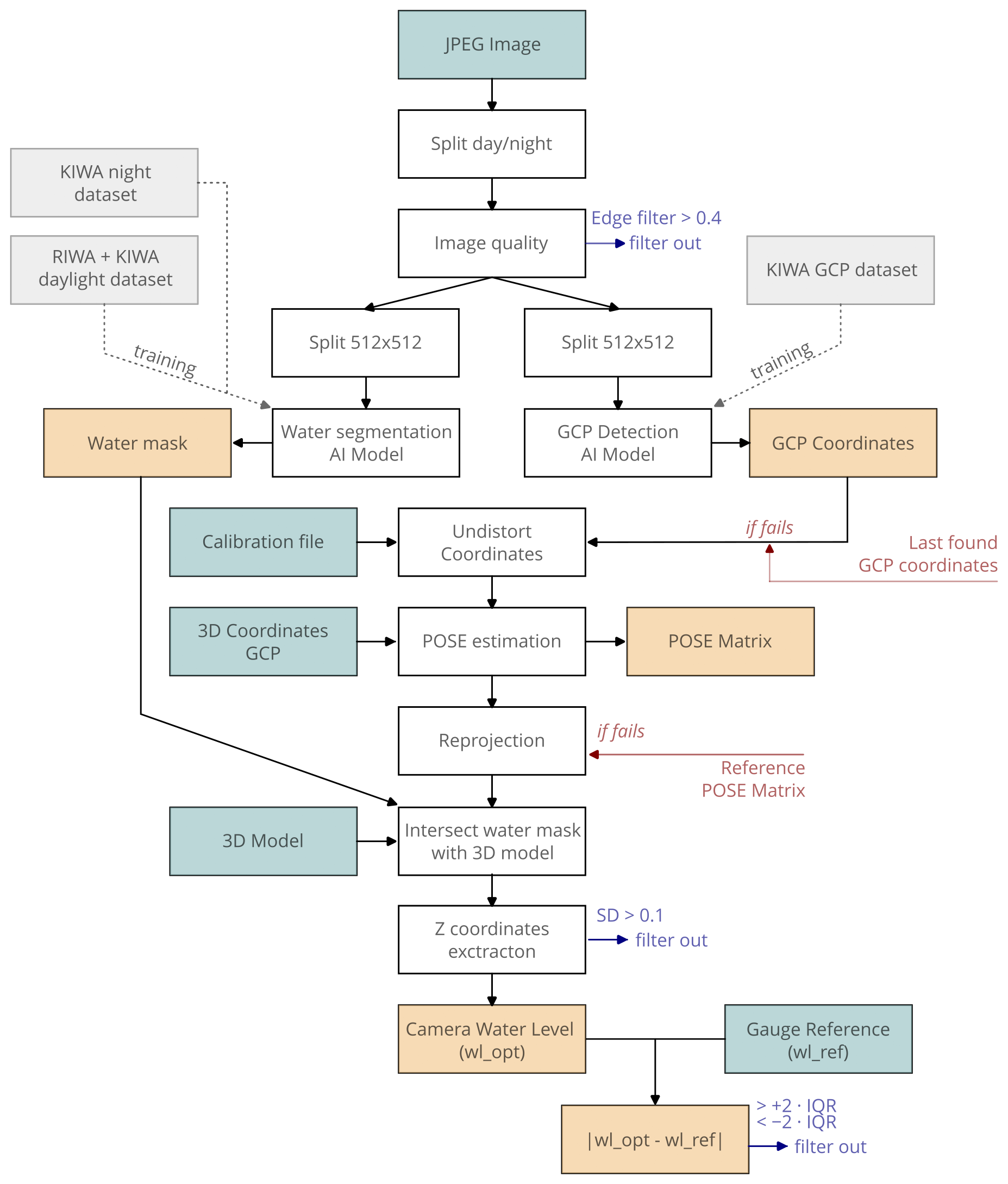
Figure B1 Flowchart summarising the complete process from image acquisition to water level determination. The chart outlines the steps from the initial JPG image captured by the camera to the final extraction of water level data.

Appendix C: ELB and GRO Results

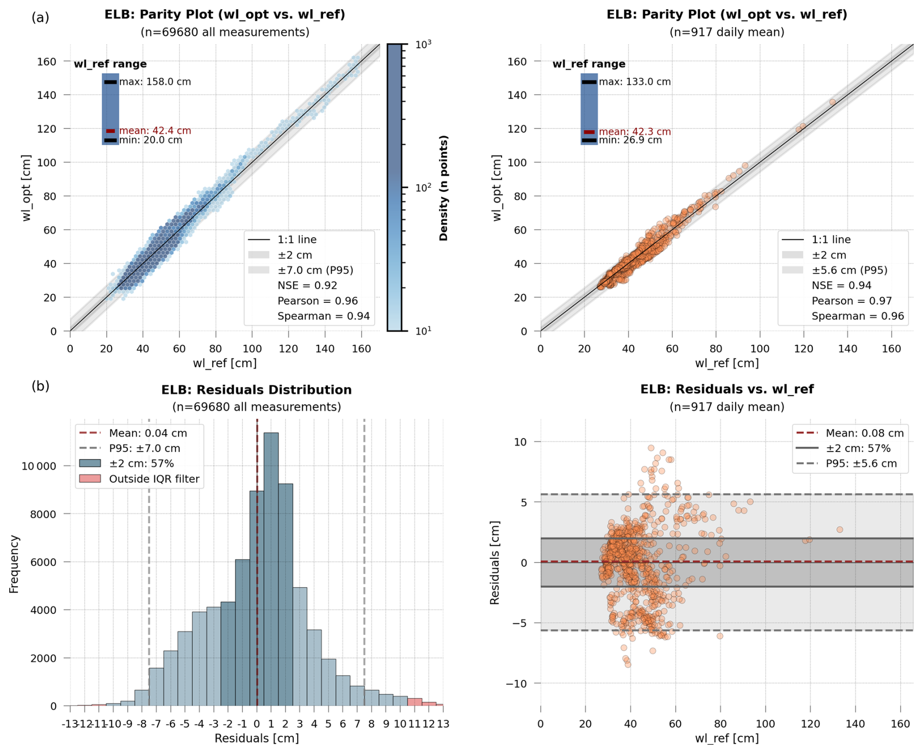
Figure C1 Validation metrics for ELB monitoring site. (a) Parity plots for all measurements (top left) and daily means (top right, scatter). (b) Bottom panels show detailed residuals analysis for all measurements: distribution histogram (left) and scatter plot vs. water level (right) for daily mean values.

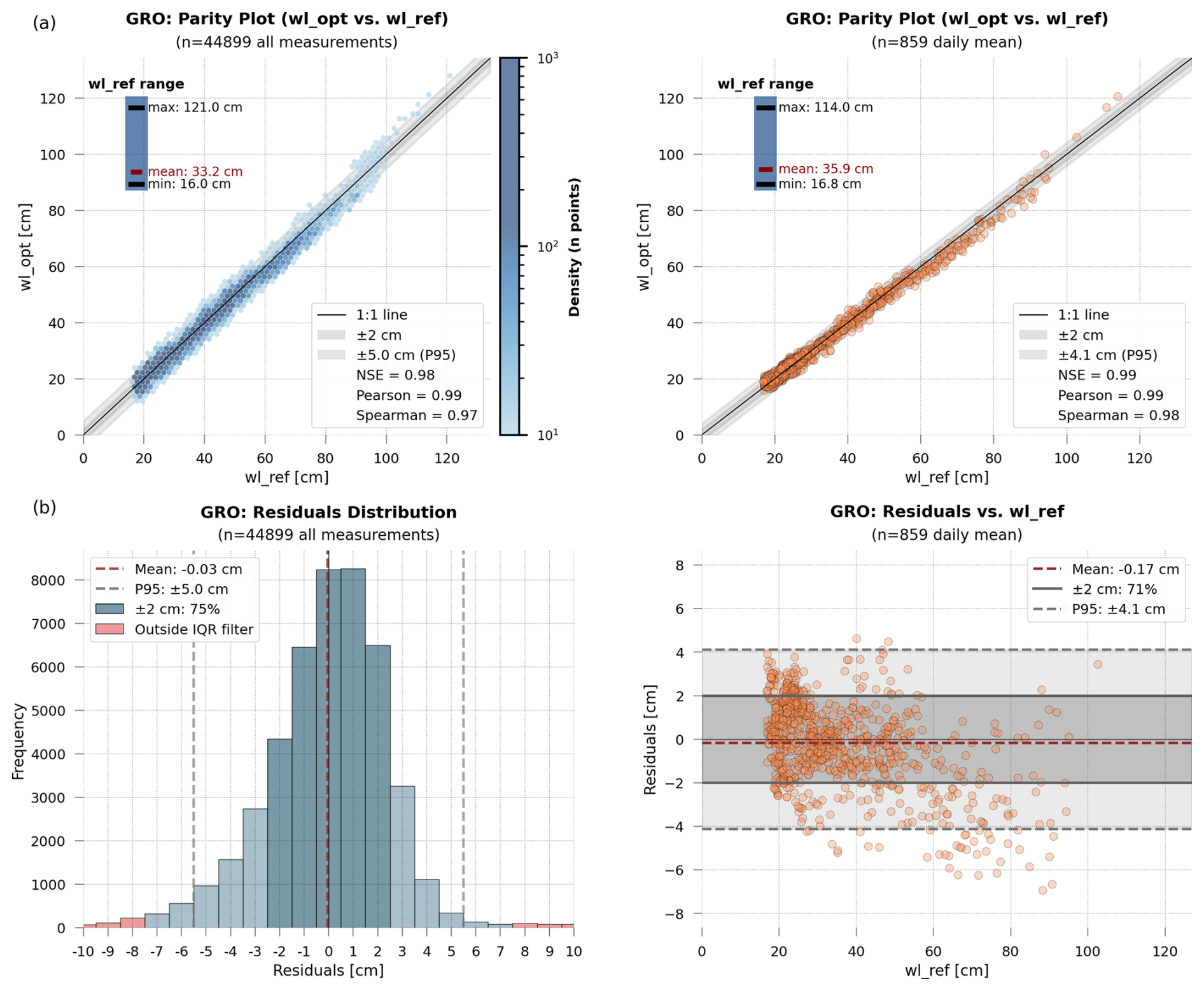
Figure C2 Validation metrics for GRO monitoring site. (a) Parity plots for all measurements (top left) and daily means (top right, scatter). (b) Bottom panels show detailed residuals analysis for all measurements: distribution histogram (left) and scatter plot vs. water level (right) for daily mean values.

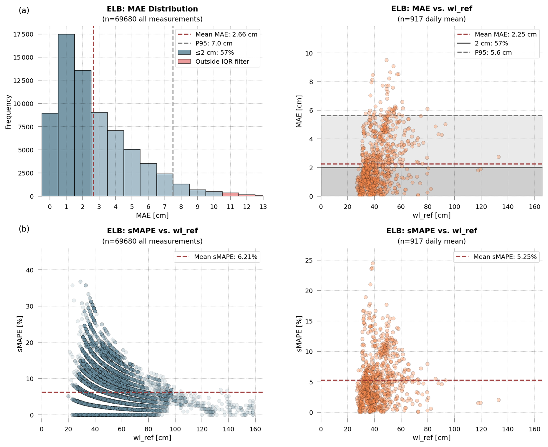
Figure C3 Error metrics for ELB monitoring site. (a) MAE distribution (top left) and MAE vs. water level (top right) for all measurements and daily means. (b) sMAPE vs. water level (bottom) for all measurements (left) and daily means (right).

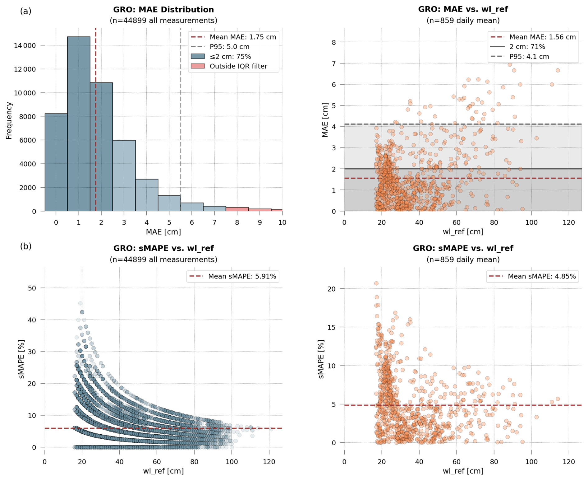
Figure C4 Error metrics for GRO monitoring site. (a) MAE distribution (top left) and MAE vs. water level (top right) for all measurements and daily means. (b) sMAPE vs. water level (bottom) for all measurements (left) and daily means (right).

Figure C5 Automated water level measurement at peak flow conditions (ELB, December 2023). The image shows the automated identification of ground control points (GCPs, crosses), the segmented water body boundary (blue line), and the upper contour segment used for water level calculation (red line).

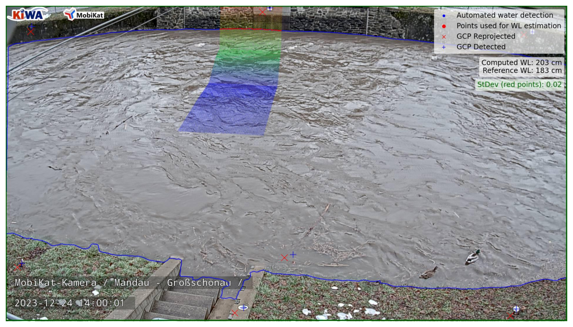
Figure C6 Automated water level measurement at peak flow conditions (GRO, December 2023). The image shows the automated identification of ground control points (GCPs, crosses), the segmented water body boundary (blue line), and the upper contour segment used for water level calculation (red line).