Technical note: Benefits of Bayesian estimation of model parameters in a large hydrological model ensemble

Quantifying and mitigating parametric and structural uncertainties in hydrological models are crucial to accurately understand and predict the rainfall-runoff process. Despite recent advances in Bayesian approaches for quantifying structural uncertainty using very large hydrological model ensembles, the simultaneous quantification of both parametric and structural uncertainties has yet to be implemented since previous works on large model ensembles have relied on deterministic optimization of parameters. Here we present the potential benefits of Bayesian estimation of parametric uncertainty within a large hydrological model ensemble. We find that Bayesian estimation of model parameters (more generally, change in calibration methods) potentially influences the interpretation of model comparisons. Specifically, Bayesian parametric uncertainty quantification greatly benefits complex models with many parameters, thereby affecting discussions of the appropriate level of model complexity. We also find that Bayesian parametric uncertainty quantification does not substantially improve multi-model hydrological predictions. The adverse effects of parameter misspecification in individual models are effectively mitigated by combining models with diverse structures. Thus, the high computational cost of Bayesian parameter estimation is not paid for to improve rainfall-runoff analysis in a large hydrological model ensemble.

1 Introduction

Hydrological models are essential tools to simulate the relationship between meteorological conditions and runoff in river basins. Quantifying and mitigating uncertainties in these models can greatly contribute to the accurate flood and drought prediction, water resources management, and climate change assessment. Assuming minimal error in input data, uncertainties in hydrological models can be broadly classified into two categories: parametric uncertainty and structural uncertainty (e.g., Beven, 2005; Gupta et al., 2012). While parametric uncertainty arises from the misspecification of model parameters, which are coefficients of equations represented in the model, structural uncertainty originates from the specification of the equations themselves. The quantification and mitigation of both parametric and structural uncertainties based on hydrological observations, particularly river discharge data, remain grand challenges in hydrology.

Mitigating parametric uncertainty has been extensively investigated in hydrology. Early research largely focused on estimating a single set of parameters that minimized the cost function measuring the fit between simulation and observation. In this paper, we refer these approaches as deterministic optimization. A wide variety of gradient-based and evolutionary algorithms have been applied to this task (e.g., Duan et al., 1993; Tolson and Shoemaker, 2007; Fowler et al., 2018; Qin et al., 2016, among others). Deterministic optimization methods suffer from equifinality (Beven, 2006), in which multiple combinations of parameters reproduce observations equally well, and degrade the accuracy of simulating unseen data. Bayesian estimation, by contrast, explicitly produces posterior probability distributions based on observations and prior knowledge of parameters. This approach offers several advantages: it can address equifinality (Vrugt et al., 2008a), enables probabilistic forecasting (e.g., Mai et al., 2025), and consider errors in data such as rainfall and river discharge measurements (e.g., Vrugt et al., 2008b). The golden standard of Bayesian estimation is Markov Chain Monte Carlo (MCMC; Hastings, 1970; Geman and Geman, 1984). In hydrology, the DiffeRential Evolution Adaptive Metropolis (DREAM) algorithm (Vrugt et al., 2008c; Laloy and Vrugt, 2012) has been widely used as a variant of MCMC algorithms. While applying MCMC to hydrological models is computationally expensive, sequential data assimilation offers a computationally cheap alternative to estimate posterior distributions of model parameters and state variables (e.g., Moradkhani et al., 2005; Vrugt et al., 2013; Sawada, 2022).

A common approach to mitigating structural uncertainty in process-based hydrological models is the applications of machine-learning, which can provide fully data-driven modeling (e.g., Kratzert et al., 2018, 2019) and correct the bias of process-based models (e.g., Funato and Sawada, 2026). These methods are intrinsically deterministic and remain subject to equifinality. Large hydrological model ensembles, such as Modular Assessment of Rainfall-Runoff Models Toolbox (MARRMoT; Knoben et al., 2019) and Raven (Craig et al., 2020) opened the door to easily perform Bayesian uncertainty quantification of model structure. Previous works employed Generalized Likelihood Uncertainty Estimation (GLUE)-like methods (Beven and Binley, 1992), in which “reasonably good” models are selected based on predefined performance thresholds to identify equally plausible models within a large multi-model ensemble. For instance, Knoben et al. (2020) evaluated 36 hydrological models across 559 river basins using MARRMoT and identified a high degree of structural equifinality. Knoben et al. (2025) further demonstrated that this high equifinality can be mitigated by considering sampling uncertainty in evaluation data. Chlumsky et al. (2021) performed simultaneous calibration of model structures and parameters (see also Mai et al., 2020). They revealed a high degree of equifinality within hydrological models implemented in the Raven framework. Although these works on large samples of hydrological models have advanced the quantification of structural uncertainty, they relied on deterministic parameter optimization. Therefore, they did not explicitly consider parametric uncertainty in the Bayesian way. It has yet to be clarified how Bayesian quantification of parametric uncertainty benefits large hydrological model ensemble-based assessment of structural uncertainty.

To address this research gap, we performed MCMC-based parametric uncertainty quantification for 17 hydrological models with different structures across 51 river basins, thereby enabling Bayesian estimation of both parametric and structural uncertainty. We then examined scientific and practical benefits of applying Bayesian estimation of model parameters in a large model ensemble. Specifically, we posed the following research questions:

• Scientific benefits. Does Bayesian estimation of model parameters (or, more broadly, changes in calibration methods) potentially affect the interpretation of model comparisons?

• Practical benefits. Does Bayesian estimation of model parameters improve the accuracy of rainfall-runoff simulations in a large hydrological model ensemble? Is this improvement sufficient to justify the large computational cost of MCMC?

2 Method

2.1 Hydrological model

We used MARRMoT v1.3 (Knoben, 2019). MARRMoT includes 46 lumped conceptual hydrological models with a wide range of complexities. The models are driven by daily total precipitation, daily mean temperature, and daily mean potential evapotranspiration, and they estimate daily basin-averaged runoff. From the 46 available models, we selected models with IDs 02, 03, 04, 06, 07, 10, 11, 12, 13, 17, 18, 21, 24, 27, 30, and 31 (see the Supplement of Knoben et al., 2019 for model details). These 17 models were chosen to preserve diversity in model complexity while minimizing the total computational cost, since Bayesian estimation of model parameters is computationally expensive. First, we decided not to use models whose MCMC computation takes longer than 2 d in our workstation. Many higher ID models were excluded in this decision. Second, we excluded models which achieved lower performance in our previous work (Sawada et al., 2022). The models with IDs 01, 14, 20, 22, and 23 were excluded. Lastly, we did not use multiple similar structure models.

2.2 Parameter estimation

2.2.1 Deterministic optimization

As a deterministic optimization method, we used the Nelder-Mead algorithm (Nelder and Mead, 1965). We performed the deterministic parameter optimization for each model in each basin. We used the fminsearchbnd function in MATLAB to search parameter sets which maximize Kling-Gupta Efficiency (KGE: Gupta et al., 2009). Parameter ranges were specified according to the original setting of MARRMoT (see Knoben et al., 2019). Although our optimization method is a classical method and may be less capable of avoiding local minima than modern evolutionary algorithms (e.g., Duan et al., 1993; Tolson and Shoemaker, 2007), we have found that it achieved high performance in our testbed (Sawada et al., 2022; see Sect. 3).

2.2.2 Bayesian optimization

For Bayesian optimization, we adopted the method proposed by Liu et al. (2022). As the MCMC method, we used the DiffeRential Evolution Adaptive Metropolis (DREAM) algorithm (Vrugt et al., 2008c; Laloy and Vrugt, 2012). While mean squared error is usually used as the formal likelihood function in the DREAM algorithm and many other MCMC applications, the informal likelihood function such as KGE is used for deterministic optimization. In our work, we will compare MCMC and deterministic optimization, so that it is necessary to use the same likelihood measure for both methods. Liu et al. (2022) proposed using KGE as an informal likelihood function. Because KGE ranges from −infinity to one, Liu et al. (2022) applied a gamma density function to handle negative KGE values and developed a proper informal likelihood for the DREAM algorithm. To use KGE in our MCMC algorithm, we used the method of Liu et al. (2022). We used the MATLAB implementation of DREAM (https://github.com/Zaijab/DREAM, last access: 30 November 2026). From the resulting Markov chains, we sampled 200 parameter sets to represent the posterior distribution of model parameters. Besides the use of the KGE-based informal likelihood function, we used the default hyperparameter setting in this implementation. The numbers of chains and maximum iterations were set to 3 and 10 000, respectively. We sampled backwards from the end of the chains to avoid sampling in the burn-in period. The number of thinning intervals was set to 10. The typical computation time of MCMC to estimate posterior parameter distributions for 17 models in a single river basin using a single Intel Xeon Gold 6348 CPU processor is 85 h.

2.3 Bayesian model averaging

To evaluate the practical benefits of Bayesian parametric uncertainty quantification in a large hydrological model ensemble, we combined models with different structures and parameters into a single prediction using Bayesian Model Averaging (BMA).

First, we combined 17 models calibrated by deterministic optimization. Let the quantity of interest generated by the kth model with deterministically optimized parameters, M_k(θ_DO,k), be denoted as Δ_k, where θ_DO,k represents the optimized parameters of the kth model. In this study, Δ_k is runoff in the validation period (see Sect. 3). Given observation y, the posterior mean of the quantity of interest is:

$$\begin{array}{}\text{(1)}& E\left[\mathrm{\Delta }|\mathit{y}\right]=\sum _k^N{w}_k{\mathrm{\Delta }}_k\end{array}$$

with model weights defined as:

$$\begin{array}{}\text{(2)}& \begin{array}{rl}{w}_k& =P\left(\left.M_k\left({\mathit{\theta }}_{\mathrm{DO},k}\right)\right|\mathit{y}\right)\\ & ={\displaystyle \frac{P\left(\left.\mathbf{y}\right|M_k\left({\mathit{\theta }}_{\mathrm{DO},k}\right)\right)P\left(M_k\right({\mathit{\theta }}_{\mathrm{DO},k})}{{\sum }_{i=\mathrm{1}}^{N}P\left(\left.\mathit{y}\right|M_i\left({\mathit{\theta }}_{\mathrm{DO},i}\right)\right)P\left(M_i\right({\mathit{\theta }}_{\mathrm{DO},i})}}\end{array}\end{array}$$

where N is the total number of models (=17 in this case). y should be recognized as river discharge observation in a calibration period. Equation (1) indicates that the posterior mean is a weighted average of all model outputs, with weights proportional to their posterior probabilities. We parameterized the weights w_k using KGE:

$$\begin{array}{}\text{(3)}& w_k={\displaystyle \frac{\exp \left(-\left({\mathrm{KGE}}_{\max }-\mathrm{KGE}\left(M_k\left({\mathit{\theta }}_{\mathrm{DO},k}\right)\right)\right)\right)}{\sum _{i=\mathrm{1}}^N\exp \left(-\left({\mathrm{KGE}}_{\max }-\mathrm{KGE}\left(M_i\left({\mathit{\theta }}_{\mathrm{DO},i}\right)\right)\right)\right)}}\end{array}$$

where KGE_max is the maximum KGE among the N models, and KGE(M_k(θ_DO,k)) is the KGE of the kth model. In this paper, this averaging of hydrological models calibrated by deterministic optimization is specifically referred to as Bayesian Model Averaging (BMA).

Next, we compared the individual models calibrated by deterministic optimization with those calibrated by MCMC. To do so, we sampled 200 parameter sets from the posterior distributions, ran models with those parameter sets, and then combined these 200 hydrological simulations by Bayesian model averaging. The performance is insensitive to the number of the sampled parameters if it is larger than 100 (not shown). Define the quantity of interest generated by the kth model with the lth parameter set, M_k(θ_l), as Δ_k,l. Similar to model averaging, the posterior mean of the quantity of interest estimated by the kth model, Δ_k follows:

$$\begin{array}{}\text{(4)}& E\left[{\mathrm{\Delta }}_k|\mathit{y}\right]=\sum _l^M{w}_l{\mathrm{\Delta }}_{k,l}\end{array}$$

with weights:

$$\begin{array}{}\text{(5)}& w_l={\displaystyle \frac{\exp \left(-\left({\mathrm{KGE}}_{\max ,k}-\mathrm{KGE}\left(M_k\left({\mathit{\theta }}_l\right)\right)\right)\right)}{{\sum }_{i=\mathrm{1}}^M\exp \left(-\left({\mathrm{KGE}}_{\max ,k}-\mathrm{KGE}\left(M_k\left({\mathit{\theta }}_i\right)\right)\right)\right)}}\end{array}$$

where M is the total number of parameter sets (i.e. 200), KGE_max,k is the maximum KGE among the M parameter sets of the kth model. This averaging within a single model with different parameters is referred to as Bayesian Parameter Averaging (BPA).

Finally, we averaged all models and parameter sets. In this case, the posterior mean of the quantity of interest is:

$$\begin{array}{}\text{(6)}& E\left[\left.\mathrm{\Delta }\right|\mathit{y}\right]=\sum _k^N\sum _l^M{w}_{k,l}{\mathrm{\Delta }}_{k,l}\end{array}$$

with weights:

$$\begin{array}{}\text{(7)}& w_{k,l}={\displaystyle \frac{\exp \left(-\left({\mathrm{KGE}}_{\max ,k,l}-\mathrm{KGE}\left(M_k\left({\mathit{\theta }}_l\right)\right)\right)\right)}{{\sum }_{i=\mathrm{1}}^N{\sum }_{j=\mathrm{1}}^M\exp \left(-\left({\mathrm{KGE}}_{\max ,k,l}-\mathrm{KGE}\left(M_i\left({\mathit{\theta }}_j\right)\right)\right)\right)}}\end{array}$$

where ${\mathrm{KGE}}_{\max ,k,l}$ is the maximum KGE among all models and parameter combinations. This joint averaging is called Bayesian Model and Parameter Averaging (BMPA).

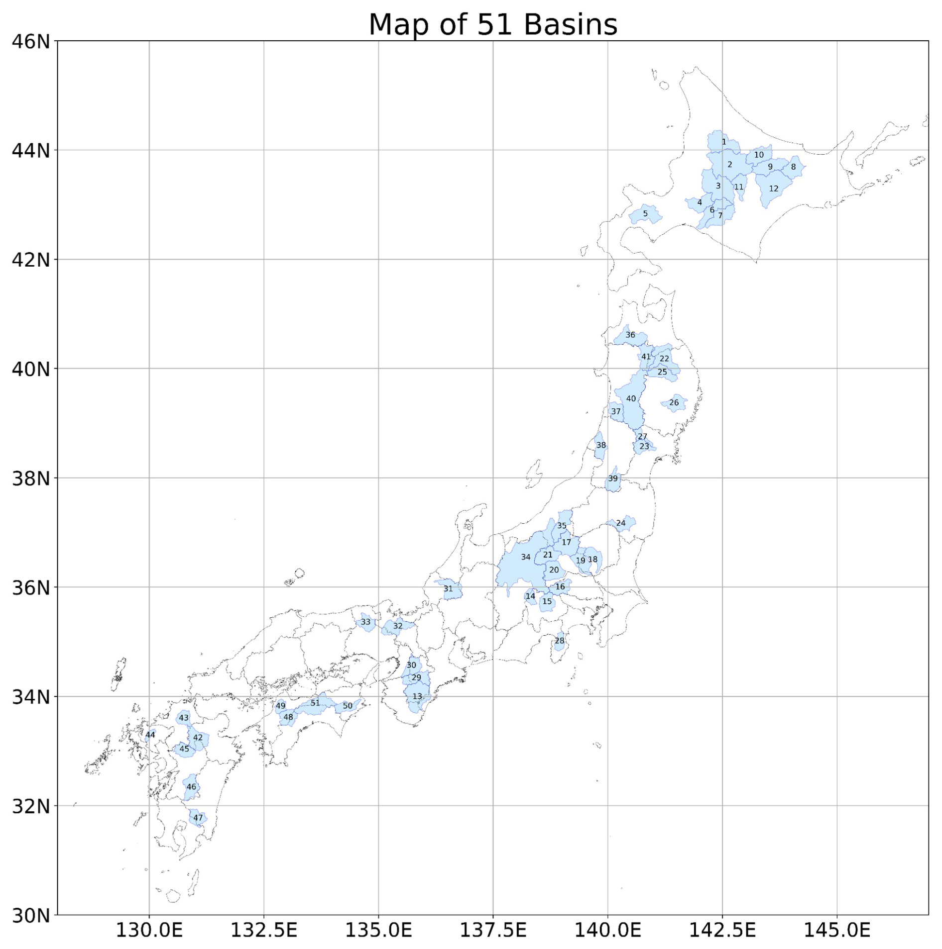
Figure 1 Study area of 51 river basins.

3 Experiment design

We applied the aforementioned methods to 51 river basins in Japan (Fig. 1). We used meteorological forcings from the Multi-model Ensemble for Robust Verification of hydrological modeling in Japan (MERV-Jp) dataset (Sawada et al., 2022; Sawada and Okugawa, 2026). While MERV-Jp originally includes 135 gauges' observations corresponding to 135 river basins, some of them are the subset of the other larger basins. In this paper, we use one of those overlapping river basins. Also, we excluded river basins whose discharge records were shorter than 25 years. Consequently, the number of river basins in this study is smaller than that in the original MERV-Jp work (Sawada et al., 2022). Daily discharge data in MERV-Jp have missing values. The likelihood function (i.e., KGE) is computed only on days when river discharge data is available. There are no missing values in our forcing inputs. The river basins shown in Fig. 1 cover a wide range of climatic, soil, land-use, anthropogenic, and topographic conditions. Sawada et al. (2022) reported that 44 deterministically calibrated models in MARRMoT achieved high accuracy to reproduce observed runoff. The best KGEs in 44 models exceeded 0.7 in nearly all basins, which are comparable to those reported in other large model ensemble studies across different regions (e.g., Knoben et al., 2020). Therefore, our findings are expected to be transferable to similar studies in the context of large hydrological model ensembles.

The study period spans 1986–2015. Two calibration periods were considered: a 5-year calibration period representing data-rich conditions, and a 1-year calibration period representing data-poor conditions. In the 5-year calibration scenario, the initial 5-year (1986-1990) data were used for calibration with both deterministic optimization and MCMC, and the remaining 25-year (1991–2015) data were used for evaluation. In basins where complete discharge records were unavailable for 1986–1990, the calibration period was shifted to ensure a continuous 5-year record, which slightly reduced the validation period. For instance, if a complete discharge record is unavailable for 1987, we extend the calibration period to 1986–1991 to evaluate models by 5-year long observation (i.e., observation in 1986, 1988, 1989, 1990, and 1991). In this case, the remaining 24-year (1992–2015) data were used for evaluation, so that the validation period is slightly shortened. We performed the shift of the calibration period in 8 river basins. We used the same 5-year data for model spin-up, resulting in a 10-year model integration for each parameter evaluation step. In the 1-year calibration scenario, we applied the same 5-year data spin-up, followed by evaluation of parameters in the subsequent 1-year simulation (1986 in most basins). The validation data for the 1-year calibration scenario were identical to those for the 5-year calibration scenario. Given a parameter set, we run a model from 1986 to 1990 as a spin-up. Then, using state variables at the last timestep of the spin-up period, we run a model again in 1986 and evaluate the estimated river discharge. In the validation process, we simply run a model with the estimated parameter set from 1986 to 2015 and discard results in 1986–1990 as a spin-up. Model performance was evaluated using KGE and Nash-Sutcliffe Efficiency (NSE; Nash and Sutcliffe, 1970; see also Duc and Sawada (2023) for a modern interpretation of NSE) during the validation period.

For deterministic optimization, we have 17 hydrological predictions by 17 models in 51 river basins, yielding 17 × 51 = 867 hydrographs. For Bayesian estimation of parametric uncertainty, each of the 17 models was run with 200 posterior parameter sets, producing 17 × 200 = 3400 simulations per basin. Across 51 basins, this amounted to 3400 × 51 = 173 400 hydrographs. First, we compared the performance of individual models calibrated by deterministic optimization with those calibrated by MCMC and combined by BPA (see Sect. 2.3) across all 17 models in 51 river basins, to assess if the evaluation of the model structures is affected by parameter estimation method. Second, we compared the performance of BMA and BPMA (see Sect. 2.3), to discuss the potential benefits of considering parametric uncertainty through Bayesian estimation in improving hydrological predictions.

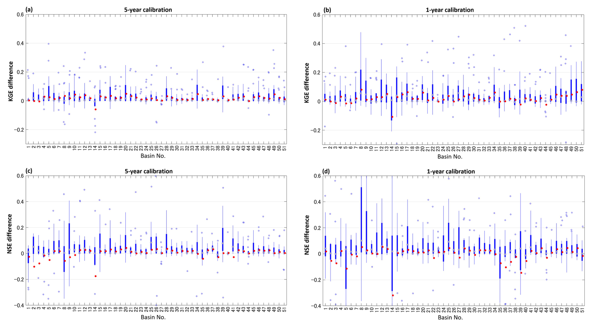
Figure 2 Differences in KGE (a, b) and NSE (c, d) between BPA and deterministically optimized models (boxplots) in 5-year (a, c) and 1-year (b, d) calibration scenarios. Red dots show the performance differences between BMPA and BMA (see Sect. 3).

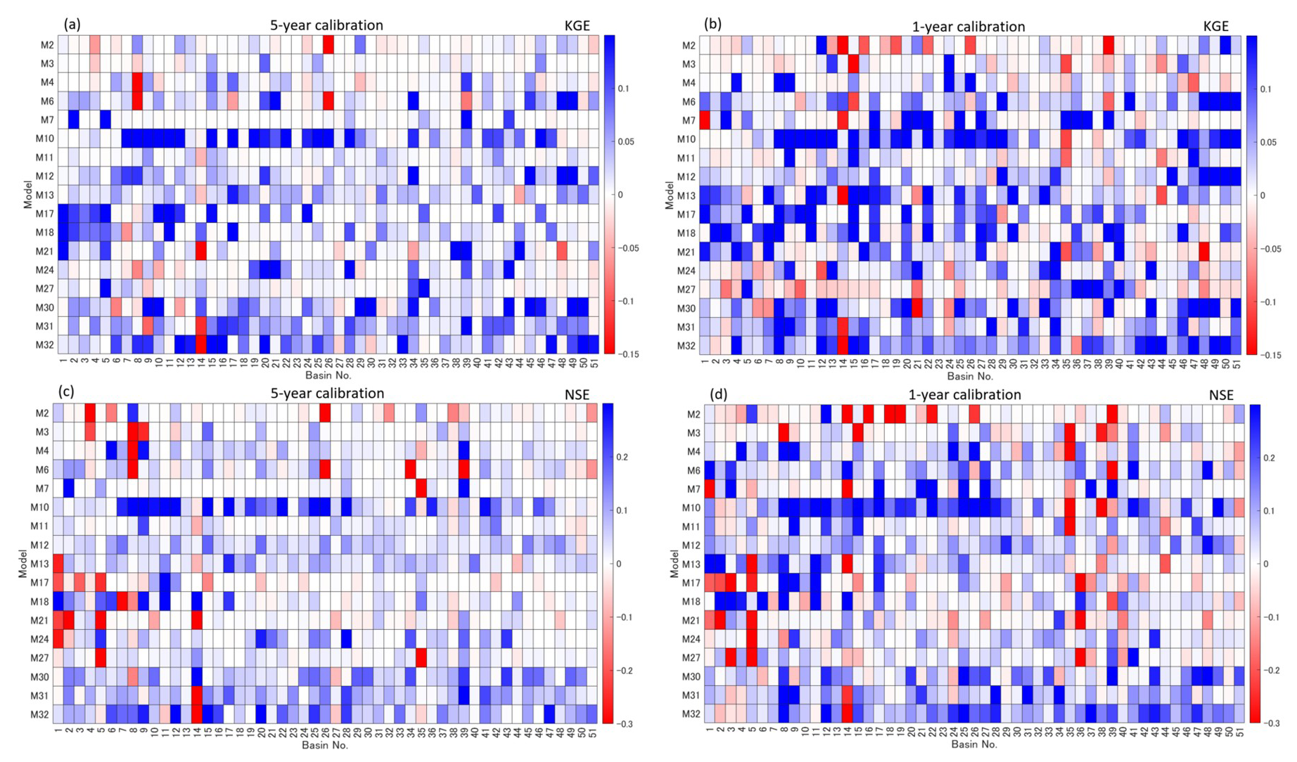
Figure 3 Differences in KGE (a, b) and NSE (c, d) between BPA and deterministically optimized models for each basin and model in 5-year (a, c) and 1-year (b, d) calibration scenarios.

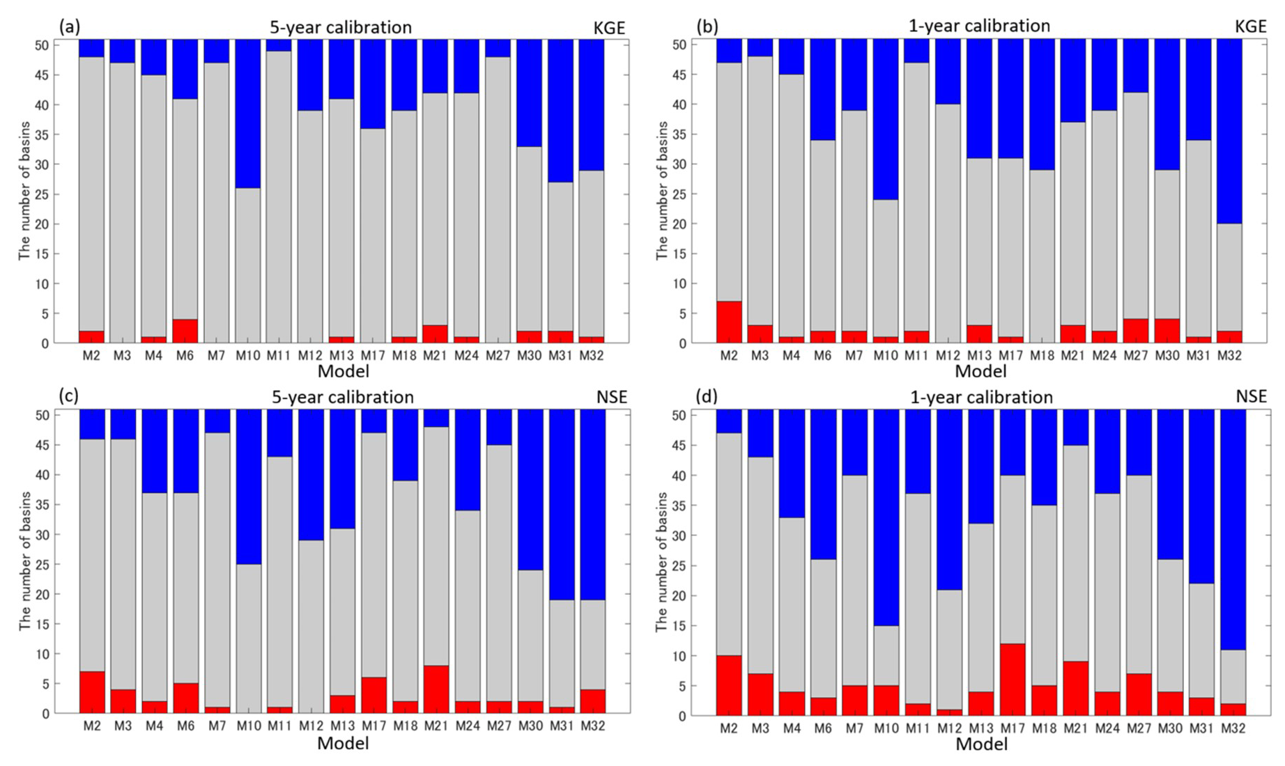
Figure 4 (a, b) The number of river basins in which (red) KGE of BPA is at least 0.05 lower than that of the deterministically optimized model, (blue) KGE of BPA is at least 0.05 higher than that of the deterministically optimized model, and (gray) the difference in KGE between BPA and the deterministically optimized model is less than 0.05, in (a) 5-year and (b) 1-year calibration scenarios. (c, d) Same as (a, b) but for NSE.

4 Results and discussions

Bayesian estimation of model parameters (i.e., BPA) systematically outperforms deterministic optimization. Boxplots of Fig. 2 show the differences in KGE and NSE between BPA and deterministically optimized models. The superiority of MCMC-based optimization is consistent with earlier findings on the DREAM (e.g., Laloy and Vrugt, 2012) algorithm. To our best knowledge, we verified this superiority within a large model ensemble for the first time. Two main factors explain this result. First, MCMC explores the parameter space more extensively to maximize KGE than deterministic optimization. Second, MCMC accounts for equifinality by sampling multiple parameter sets that reproduce observation equally well, which leads the higher robustness to unseen data. Even in the rich-data scenario (i.e., the 5-year calibration), improvements in KGE exceeds 0.2 in some models. This trend is more pronounced in the data-scarce scenario (i.e., 1-year calibration scenario). When calibration data are limited, parameter estimates are inherently uncertain, since many different parameter combinations may be able to equally explain the limited data. In such cases, Bayesian estimation is more appropriate than deterministic methods.

Figures 3 and 4 reveal that the improvements achieved by BPA over deterministically optimized models systematically appear. For instance, model ID 10 (Susannah Brook model v2; see Son and Sivapalan, 2007; Knoben et al., 2019) shows substantial gains from Bayesian parameter estimation in more than 20 river basins. Except for this model, more complex models with the larger numbers of parameters (e.g., ID 30, 31, and 32) tend to benefit more from Bayesian estimation than simpler models (e.g., ID 2, 3, and 4) (note that models with higher IDs generally correspond to greater structural complexity; see Knoben et al., 2019) especially in the data-rich scenario (i.e., 5-year calibration scenario). This indicates that models with many parameters are particularly affected by equifinality and therefore gain substantially from Bayesian parameter estimation.

Previous studies have evaluated model structures by comparing the performance of deterministically optimized models. Our results imply that such evaluations may be affected by the choice of parameter optimization methods. For instance, although results in Knoben et al. (2020) and Knoben et al. (2025) indicated that complex models with many parameters do not necessarily outperform simpler models, this conclusion may partly reflect an underestimation of the maximum potential performance of complex models due to reliance on deterministic optimization. While these complex models have been shown not to suffer from overfitting (Knoben et al., 2020), there might be room for improvement through Bayesian estimation, which explicitly addresses parameter equifinality.

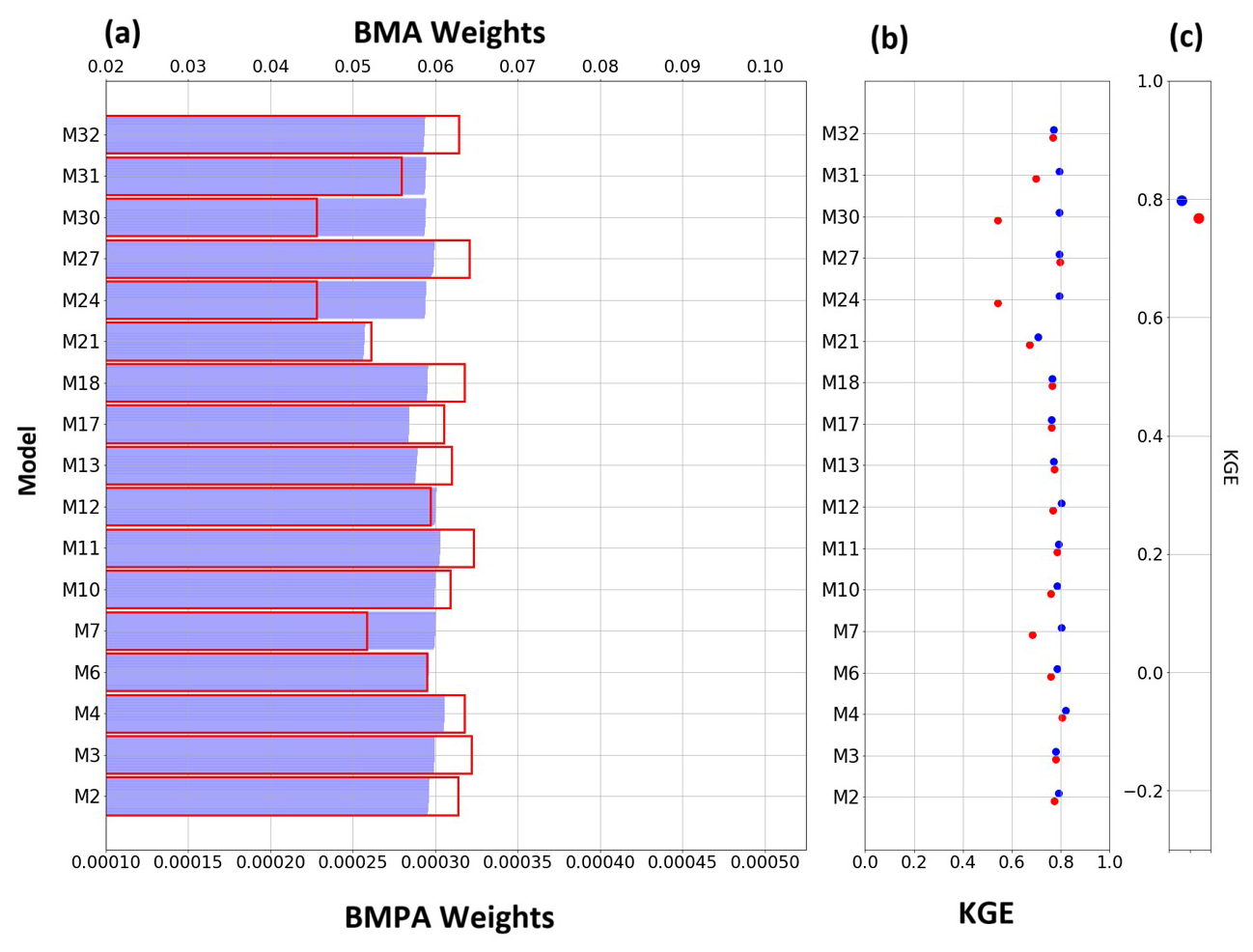
Figure 5 (a) Weights in BMA (red bars) and BMPA (blue bars). (b) KGE of BPA (blue dots) and deterministically optimized models (red dots). (c) KGE of BMPA (blue dots) and BMA (red dots). Results of basin No. 43 (see Fig. 1) are shown.

When a large number of calibrated models are available, a practical way to improve prediction accuracy is to use the (weighted) average of their outputs (e.g., Kimizuka and Sawada, 2022; Zhang and Yang, 2018). The red dots in Figure 2 show the performance differences between BPMA and BMA. Although Bayesian parameter estimation substantially improves the performance of individual models, the overall improvement from BMA to BPMA is marginal. Even in the data-scarce scenario (i.e., the 1-year calibration scenario), the improvement in KGE (NSE) by Bayesian estimation is less than 0.1 (0.05). Surprisingly, even the classic optimization method remains competitive with DREAM-based Bayesian optimization when models are combined in a large ensemble. Considering the substantial computational costs of the MCMC-based Bayesian parameter estimation, we conclude that Bayesian parametric uncertainty quantification provides limited practical benefits for improving predictions in large hydrological model ensembles.

This occurs because poorly performing models produced by deterministic optimization are assigned lower weights in the BMA framework. Figure 5 illustrates a typical case: in basin no. 43, BPA achieves 0.8 KGE for nearly all models, while some deterministically optimized models (i.e., ID 7, 21, 24, 30, and 31) perform poorly. Nevertheless, BMA remains competitive with BPMA, since the poorly performing models receive smaller weights during averaging. Therefore, the adverse effects of suboptimal calibration are effectively mitigated.

5 Conclusions

Here we performed MCMC-based parameter optimization for 17 hydrological models across 51 river basins to clarify the potential benefits of Bayesian parametric uncertainty quantifications in a large hydrological model ensemble. Scientifically, Bayesian parametric uncertainty quantification is important because it can influence the interpretation of structural uncertainty assessment. The benefits of the Bayesian parameter estimation appear systematically across models rather than randomly. Certain models gain substantial improvements, and more complex models tend to benefit more strongly than simpler models. Considering Bayesian parameter uncertainty potentially affects the discussion of the appropriate complexity of hydrological models.

Practically, Bayesian parametric uncertainty quantification does not greatly contribute to improving multi-model ensemble hydrological prediction. It implies that structural errors are larger than parametric errors in hydrological prediction. Given the high computational cost of Bayesian estimation, multi-model ensembles calibrated by deterministic optimization are sufficient in many cases.

Our analysis was limited to 17 models, fewer than in previous large ensemble studies (Knoben et al., 2020, 2025; Chlumsky et al., 2021). We had to exclude computationally expensive models in MARRMoT to make the MCMC applications feasible in this initial attempt. Future work should expand to all MARRMoT models and pursue GLUE-like assessments of structural uncertainty using Bayesian parameter uncertainty quantification by unleashing the power of high-performance computers.