Technical note: Machine learning metamodelling for global sensitivity analysis

Global sensitivity analysis (GSA) plays a central role in hydrologic modelling by supporting model understanding, diagnosis, and decision-making through the identification of influential and non-influential parameters and their interactions. Variance-based methods provide a rigorous framework for GSA but are often computationally expensive, as their estimation requires a large number of model evaluations. Metamodelling has therefore been widely adopted as a strategy to alleviate this issue, with recent advances in machine learning (ML) offering new opportunities to construct accurate and flexible surrogates for complex models. This technical note examines the practical relationship between Sobol' total-effect indices (T_i) and feature importance measures derived from ML metamodels within a hydrologic modelling context. Building on theoretical results that link T_i to permutation variable importance (PVI_i) under independence assumptions, we provide systematic numerical evidence using three hydrologic models of varying complexity (HBV, HyMod, and VIC) applied to three headwater catchments in northern Germany, together with three ML metamodels: a gradient boosting decision tree (GBDT), a neural network (NN), and a linear model (LM). The three metamodels were trained on Monte Carlo samples and used to estimate sensitivities through PVI_i and SHapley Additive exPlanations (SHAP_i). The results demonstrate that GBDT and NN metamodels reliably reproduce both the ranking and relative magnitude of T_i using PVI_i across all hydrologic models, providing clear empirical support for the theoretical connection between the two measures. In contrast, the performance of LM-based estimates depends strongly on the degree of linearity in the underlying model response. Mean absolute SHAP_i values exhibit a consistent monotonic relationship with T_i and preserve parameter rankings, while sample-specific SHAP_i values enable a distributed evaluation of sensitivities across both the parameter space and the target variable space. Overall, this study highlights ML metamodelling as a computationally efficient and conceptually sound framework for GSA in hydrologic modelling and beyond.

1 Introduction

Global sensitivity analysis (GSA) provides a systematic framework to quantify how uncertainty in model outputs can be attributed to uncertainty in model inputs, both individually and through their interactions (Saltelli et al., 2008, 2010). GSA supports model understanding, diagnosis, and decision-making by revealing dominant controls, identifying influential and non-influential parameters, and highlighting the role of interactions in complex systems. These properties make GSA particularly valuable for hydrologic modelling, where models are often nonlinear, high-dimensional, and affected by substantial uncertainty. In this context, GSA enables a sensitivity analysis based on different settings, such as the prioritization of influential input factors to inform data collection and parameter estimation efforts, or for the identification of non-influential factors that can be fixed to reduce model complexity (Saltelli and Tarantola, 2002). Sensitivity analysis facilitates the diagnosis and comparison of alternative model structures, hypotheses, and assumptions (Razavi et al., 2021; Sheikholeslami et al., 2021).

Among GSA approaches, variance-based methods provide a formal way to quantify how uncertainty in model outputs can be attributed to uncertainty in individual input factors and their interactions. Within this class of methods, Sobol’ indices describe how uncertainty in each input propagates through the model, with first-order indices measuring additive effects and total-effect indices accounting for the overall contribution of each factor, including higher-order interactions (Saltelli et al., 2010). Variance-based sensitivity analysis has been widely adopted across scientific disciplines and is commonly used as a reference for GSA (Lo Piano et al., 2021; Puy et al., 2022). A limitation of variance-based approaches is that they rely on the assumption that the variance of the model output is an adequate proxy for its uncertainty, which has motivated the development of moment-independent importance measures (Borgonovo et al., 2011). In hydrologic modelling, several studies have also highlighted important challenges in applying variance-based approaches, particularly when assessing sensitivity with respect to performance metrics. In such cases, global aggregation can obscure varying behaviours across different levels of model performance, and sensitivity estimates may vary substantially depending on the choice of performance metric and the defined parameter boundaries (Razavi and Gupta, 2015, 2016). These considerations motivate a careful and critical use of variance-based sensitivity analysis in hydrologic applications, while reinforcing its role as a rigorous and informative sensitivity framework. While these challenges are particularly evident in hydrologic modelling, they are not exclusive to it and extend to complex models in general.

A major practical limitation of variance-based GSA is its computational cost. Accurate estimation of total-effect indices typically requires a large number of model evaluations, scaling with both the number of uncertain inputs and the sample size required for convergence (Saltelli et al., 2010; Puy et al., 2022). For computationally expensive or high-dimensional models, these costs can become prohibitive, revealing the paradox of GSA: the models that would benefit most from GSA are typically those for which a full analysis is computationally infeasible. To alleviate this issue, metamodelling has long been proposed as a strategy to replace the original model with a computationally efficient approximation, also referred to as surrogate modelling (Saltelli et al., 2008; Razavi et al., 2012). Metamodels can enable GSA at a fraction of the original cost, but their reliability in yielding accurate sensitivity estimates critically depends on the ability of the surrogate to faithfully reproduce the input–output relationship of the original model.

Recent advances in machine learning (ML) offer new opportunities for metamodelling in the context of GSA. ML algorithms are particularly well suited to approximate complex, nonlinear relationships in high-dimensional spaces, making them attractive candidates for metamodelling. In a comprehensive review, Antoniadis et al. (2021) discussed the use of random forests for GSA and highlighted the close conceptual link between feature importance measures and sensitivity indices. In particular, for a given ML algorithm, permutation variable importance quantifies the increase in prediction error induced by breaking the association between an input and the model output, a mechanism that is closely related to the notion of variance-based total-effect sensitivity. This connection suggests that ML-based feature importance measures may provide an alternative route to estimate sensitivities through metamodelling, provided that the surrogate accurately reproduces the behaviour of the original model.

The objective of this technical note is to examine the practical relationship between variance-based total-effect sensitivity indices (Homma and Saltelli, 1996) and feature importance measures derived from ML metamodels within a hydrologic modelling context. Building on theoretical results that link total-effect indices and permutation variable importance under the assumption that the input factors have independent probability distributions, we provide systematic numerical evidence using three hydrologic models with varying structural complexity. We assess the ability of different ML metamodels to reproduce variance-based sensitivities, analyse the conditions under which this approximation is reliable, and explore alternative sensitivity measures enabled by ML surrogates. By doing so, this work aims to clarify the role of ML metamodelling as a computationally efficient and conceptually sound framework for GSA in hydrologic modelling.

Before presenting the specific objectives and details of the numerical experiment, the next section introduces the mathematical preliminaries that underpin the rationale of this work. We present the key concepts of variance-based sensitivity analysis and permutation variable importance, complemented by intuitive explanations to facilitate interpretation. While this section relies on probabilistic and statistical reasoning that may be challenging for readers less familiar with these topics, it is included to ensure clarity and transparency and to establish a solid foundation for the methodological developments and numerical results that follow.

2 Mathematical preliminaries

This section presents the mathematical preliminaries underlying this work. Section 2.1 and 2.3 introduce the theoretical definitions of variance-based sensitivity indices and permutation variable importance, respectively, while Sect. 2.2 and 2.4 describe their practical estimation. This distinction between theoretical definition and practical estimation is reflected in the notation: quantities without a hat denote theoretical measures, whereas their estimators are denoted with a hat.

2.1 Variance-based sensitivity analysis

Given a deterministic model of the form Y=f(X), where Y is a scalar model output and $\mathit{X}=(X_{\mathrm{1}},\mathrm{\dots },X_p)$ is a vector of p uncertain input factors, variance-based sensitivity analysis aims to quantify how the uncertainty in Y can be attributed to the uncertainties in the individual input factors and their interactions.

The first-order Sobol' index of the i-th factor, X_i, is defined as e.g, Saltelli et al. (2008, 2010):

$$\begin{array}{}\text{(1)}& S_{\mathrm{i}}={\displaystyle \frac{{\mathrm{Var}}_{X_{\mathrm{i}}}\left({\mathbb{E}}_{X_{\sim i}}\right[Y\left|X_{\mathrm{i}}\right])}{\mathrm{Var}\left(Y\right)}}\end{array}$$

where Var(.) and 𝔼[.] are the variance and expectation operators, respectively, and X_∼i denotes the vector of all input factors except X_i.

S_i is normalized between 0 and 1, with larger values indicating a stronger additive effect of X_i on the model output. The inner expectation in ${\mathrm{Var}}_{X_{\mathrm{i}}}\left({\mathbb{E}}_{X_{\sim i}}\right[Y\left|X_{\mathrm{i}}\right])$ represents the conditional expectation of Y given X_i, and intuitively averages out the effect of all other factors, isolating the contribution of X_i. The outer variance measures how much this contribution varies across all possible values of X_i.

When ${\sum }_{i=\mathrm{1}}^p{S}_{\mathrm{i}}=\mathrm{1}$, the model is additive, which means that Var(Y) can be decomposed as the sum of all the first-order effects as there are no interactions among the input factors. However, in the presence of non-negligible interactions ${\sum }_{i=\mathrm{1}}^p{S}_{\mathrm{i}}\le \mathrm{1}$, and the first-order indices would not be informative enough to quantify sensitivities. This is generally the case for any real-world model.

The total-effect Sobol' index of X_i measures the total contribution of X_i to the output variance, including all interactions with other factors, and is given by e.g. Homma and Saltelli (1996):

$$\begin{array}{}\text{(2)}& T_{\mathrm{i}}=\mathrm{1}-{\displaystyle \frac{{\mathrm{Var}}_{X_{\sim i}}\left({\mathbb{E}}_{X_{\mathrm{i}}}\right[Y\left|{\mathit{X}}_{\sim i}\right])}{\mathrm{Var}\left(Y\right)}}\end{array}$$

One intuitive interpretation is that the term ${\mathrm{Var}}_{X_{\sim i}}\left({\mathbb{E}}_{X_{\mathrm{i}}}\right[Y\left|{\mathit{X}}_{\sim i}\right])$ represents the variance explained by all factors except X_i. Subtracting this from the total variance Var(Y) isolates the contribution of X_i and all its interactions. T_i satisfies the condition $S_{\mathrm{i}}\le T_{\mathrm{i}}\le \mathrm{1}$, and for additive models S_i=T_i as there are no factor interactions.

Further details and a complete derivation of the Sobol' indices can be found, for example, in Saltelli et al. (2008). It is important to note that the definitions presented above assume that the input factors have independent probability distributions. Under this assumption, Var(Y) can be uniquely decomposed into contributions from individual factors and their interactions. When the inputs are not independent, this decomposition is no longer unique. Extensions of Sobol' indices to dependent inputs have been proposed in the literature (e.g., Chastaing et al., 2015; Il Idrissi et al., 2021; Jacques et al., 2006; Kucherenko et al., 2017; Li et al., 2010; Mara et al., 2015), but these are beyond the scope of this work.

2.2 Estimation of Sobol' indices

The estimation of Sobol' indices requires two essential components: a sampling strategy to generate points in the space of the input factors, and an estimator to compute sensitivity (Lo Piano et al., 2021). Here, we follow the Monte Carlo–based numerical approach recommended by Saltelli et al. (2010) to estimate S_i and T_i using a single set of model evaluations. For a comprehensive overview of available estimators, we refer the reader to Puy et al. (2022).

Let A and B be two independent sampling matrices, each containing n realizations of the p input factors. For each input factor, we construct the hybrid matrix ${\mathbf{A}}_B^{\left(i\right)}$ by replacing the ith column of A with the corresponding column of B. S_i and T_i can be estimated as:

$$\begin{array}{}\text{(3)}& {\displaystyle }{\widehat{S}}_{\mathrm{i}}={\displaystyle \frac{\frac{\mathrm{1}}{n}{\sum }_{v=\mathrm{1}}^{n}f(\mathbf{B}{)}_v\left[f{\left({\mathbf{A}}_B^{\left(i\right)}\right)}_v-f(\mathbf{A}{)}_v\right]}{\mathrm{Var}\left(Y\right)}}\text{(4)}& {\displaystyle }{\widehat{T}}_{\mathrm{i}}={\displaystyle \frac{\frac{\mathrm{1}}{n}{\sum }_{v=\mathrm{1}}^n{\left[f(\mathbf{A}{)}_v-f({\mathbf{A}}_B^{\left(i\right)}{)}_v\right]}^{\mathrm{2}}}{\mathrm{2}\mathrm{Var}\left(Y\right)}}\end{array}$$

In the previous expressions, Var(Y) can be estimated as Puy et al. (2022):

$$\begin{array}{}\text{(5)}& \widehat{\mathrm{Var}}\left(Y\right)={\displaystyle \frac{\mathrm{1}}{\mathrm{2}n-\mathrm{1}}}\sum _{v=\mathrm{1}}^n\left[\left(f\right(\mathbf{A}{)}_v-f_{\mathrm{0}}{)}^{\mathrm{2}}+\left(f\right(\mathbf{B}{)}_v-f_{\mathrm{0}}{)}^{\mathrm{2}}\right]\end{array}$$

where $f_{\mathrm{0}}=\frac{\mathrm{1}}{\mathrm{2}n}{\sum }_{v=\mathrm{1}}^n\left[f(\mathbf{A}{)}_v+f(\mathbf{B}{)}_v\right]$. Here and throughout the remainder of the paper we employ the hat notation for estimators.

Equation (3) was originally proposed in Saltelli et al. (2010) as an improvement to previous approaches, although it has been outperformed by better practices, see e.g. Azzini et al. (2021). Equation (4) was introduced in Jansen (1999) and represents the best practice thus far to estimate T_i. As a result, the estimation of S_i and T_i based on the triplet of matrices A, B, and ${\mathbf{A}}_B^{\left(i\right)}$ has a total cost of n(p+2) simulations: 2n simulations are required for matrices A and B, and pn simulations for the hybrid matrices ${\mathbf{A}}_B^{\left(i\right)}$.

2.3 Permutation variable importance

Let Y be a real-valued random variable and $\mathit{X}=(X_{\mathrm{1}},\mathrm{\dots },X_p)$ a vector of real-valued random variables. We assume that X and Y are jointly distributed according to some joint distribution encoding a general relationship between X and Y, which may be deterministic or stochastic.

To assess the contribution of each variable X_i to the variability of Y, we define the modified vector ${\mathit{X}}_{\left(i\right)}=(X_{\mathrm{1}},\mathrm{\dots },X_{\mathrm{i}}^{\prime },\mathrm{\dots },X_p)$, where $X_{\mathrm{i}}^{\prime }$ is an independent replication of X_i that is also independent of Y and of all other variables. The permutation variable importance (PVI) of the ith variable is formally defined as Zhu et al. (2015); Gregorutti et al. (2017):

$$\begin{array}{}\text{(6)}& {\mathrm{PVI}}_{\mathrm{i}}=\mathbb{E}\left[(Y-\mathbb{E}[Y\left|{\mathit{X}}_{\left(i\right)}\right]{)}^{\mathrm{2}}\right]-\mathbb{E}\left[(Y-\mathbb{E}[Y\left|\mathit{X}\right]{)}^{\mathrm{2}}\right]\end{array}$$

where 𝔼[Y|X] denotes the conditional expectation of Y given X.

𝔼[Y|X] represents the best function of X for predicting Y in the least-square sense (Bertsekas and Tsitsiklis, 2008), and therefore the expression $\mathbb{E}\left[(Y-\mathbb{E}[Y\left|\mathit{X}\right]{)}^{\mathrm{2}}\right]$ corresponds to the smallest possible mean squared error (MSE) achievable if one could use the true conditional expectation as a predictor. This quantity represents the irreducible uncertainty in Y, that is, the part of its variability that cannot be explained by X, no matter what model is used.

On the other hand, the term $\mathbb{E}\left[(Y-\mathbb{E}[Y\left|{\mathit{X}}_{\left(i\right)}\right]{)}^{\mathrm{2}}\right]$ measures the expected MSE when X_i is replaced by an independent copy $X_{\mathrm{i}}^{\prime }$ and the information carried by X_i has been destroyed. Hence, PVI_i measures the increase in MSE when X_i is made independent of Y, with a large PVI_i indicating that X_i contributes substantially to predicting Y.

If we restrict our attention to the case when the dependence between X and Y is purely deterministic, the relationship between X and Y can be written as Y=f(X). This is the case of the generic model defined in the previous section. Here, $\mathbb{E}\left[Y\right|\mathit{X}]=f(\mathit{X})$, and Eq. (6) reduces to:

$$\begin{array}{}\text{(7)}& {\mathrm{PVI}}_{\mathrm{i}}=\mathbb{E}\left[\left(f\right(\mathit{X})-f({\mathit{X}}_{\left(i\right)}){)}^{\mathrm{2}}\right]\end{array}$$

PVI_i measures the average change in f(X) when the ith component is permuted. Then, if the components of X are independent, Wei et al. (2015) established the following relationship for T_i and PVI_i:

$$\begin{array}{}\text{(8)}& T_{\mathrm{i}}={\displaystyle \frac{{\mathrm{PVI}}_{\mathrm{i}}}{\mathrm{2}\mathrm{Var}\left(Y\right)}}={\displaystyle \frac{\mathbb{E}\left[\left(f\right(\mathit{X})-f\left({\mathit{X}}_{\left(i\right)}\right){)}^{\mathrm{2}}\right]}{\mathrm{2}\mathrm{Var}\left(Y\right)}}\end{array}$$

This relation constitutes an important connection between sensitivity analysis and ML: T_i is central to GSA, while PVI_i provides a model-agnostic approach widely used in explainable artificial intelligence (XAI) to quantify feature importance for ML models. Although beyond the scope of this work, interested readers are referred to the work of Benoumechiara (2019), which proposed a modified version of PVI_i to calculate S_i and provided an in-depth analysis of the dependent case using a Rosenblatt transformation of the input variables.

Based on Eq. (8), an estimator of T_i can be constructed with the matrices A, B, and ${\mathbf{A}}_B^{\left(i\right)}$ introduced in the previous section. The generation of ${\mathbf{A}}_B^{\left(i\right)}$ by replacing the i-th column of A with the i-th column of B mimics the independent replication of X_i in X_(i). Therefore, T_i can be estimated with the following expression:

$$\begin{array}{}\text{(9)}& {\widehat{T}}_{\mathrm{i}}={\displaystyle \frac{\frac{\mathrm{1}}{n}{\sum }_{v=\mathrm{1}}^n{\left[f(\mathbf{A}{)}_v-f({\mathbf{A}}_B^{\left(i\right)}{)}_v\right]}^{\mathrm{2}}}{\mathrm{2}\mathrm{Var}\left(Y\right)}}\end{array}$$

where Var(Y) can be estimated using Eq. (5).

Equation (9) is identical to the total-order estimator proposed by Jansen (1999) (see Eq. 4). Our goal now is to demonstrate how the estimation of PVI_i is carried out in practice for ML models. This provides an alternative way for estimating T_i based on ML metamodelling, which is the focus of this work.

2.4 Estimation of PVI_i

Let ${\mathcal{D}}_n=\mathit{\left\{}\right({\mathit{X}}_{\mathrm{1}},Y_{\mathrm{1}}),\mathrm{\dots },({\mathit{X}}_n,Y_n\left)\mathit{\right\}}$ denote a learning set consisting of n independent observations from the joint distribution of X and Y, where X and Y are defined as in the previous section. The goal in a regression setting is to find an estimator $\widehat{f}$ of 𝔼[Y|X] (Zhu et al., 2015; Gregorutti et al., 2017). Broadly speaking, this involves fitting a function to the learning set that minimizes a loss function of choice, thereby producing a reliable approximation of the underlying relationship between X and Y.

The most common approach to estimate PVI_i in practice is the importance measure proposed in Breiman (2001) for random forests (Antoniadis et al., 2021; Vannucci et al., 2026). Let ${\widehat{f}}_k$ denote the k-th tree in an ensemble of n_tree trees and let ${\stackrel{\mathrm{‾}}{\mathcal{D}}}_k$ be its out-of-bag (OOB) sample, namely the subset of observations not used to train that tree. The prediction error $\widehat{R}$ of ${\widehat{f}}_k$, expressed as MSE, is given by the following estimator over ${\stackrel{\mathrm{‾}}{\mathcal{D}}}_k$ (Gregorutti et al., 2017):

$$\begin{array}{}\text{(10)}& \widehat{R}\left({\widehat{f}}_k,{\stackrel{\mathrm{‾}}{\mathcal{D}}}_k\right)={\displaystyle \frac{\mathrm{1}}{\left|{\stackrel{\mathrm{‾}}{\mathcal{D}}}_k\right|}}\sum _{i:\left({\mathit{X}}_{\mathrm{i}},Y_{\mathrm{i}}\right)\in {\stackrel{\mathrm{‾}}{\mathcal{D}}}_k}(Y_{\mathrm{i}}-{\widehat{f}}_k({\mathit{X}}_{\mathrm{i}}){)}^{\mathrm{2}}\end{array}$$

where $\left|{\stackrel{\mathrm{‾}}{\mathcal{D}}}_k\right|$ is the number of samples in ${\stackrel{\mathrm{‾}}{\mathcal{D}}}_k$.

For each input factor X_i, let us now define a perturbed version of the OOB sample, denoted ${\stackrel{\mathrm{‾}}{\mathcal{D}}}_k^i$, by randomly permuting the values of X_i while keeping all other variables unchanged. The importance of X_i is then estimated through the degradation in prediction error induced by this perturbation averaged over all trees in the forest (Gregorutti et al., 2017):

$$\begin{array}{}\text{(11)}& {\widehat{\mathrm{PVI}}}_{\mathrm{i}}={\displaystyle \frac{\mathrm{1}}{n_{\text{tree}}}}\sum _{k=\mathrm{1}}^{n_{\text{tree}}}\left[\widehat{R}\right({\widehat{f}}_k,{\stackrel{\mathrm{‾}}{\mathcal{D}}}_k^i)-\widehat{R}({\widehat{f}}_k,{\stackrel{\mathrm{‾}}{\mathcal{D}}}_k\left)\right]\end{array}$$

This expression is the empirical counterpart of the theoretical definition of PVI_i presented in Eq. (6). Although random forests provide a natural setting for estimating PVI_i, the permutation principle is not restricted to this class of models. Given any regression algorithm, one may estimate the importance of X_i by evaluating the predictive performance of the fitted model $\widehat{f}$ and comparing it with the performance obtained after permuting the values of X_i. This general procedure is a model-agnostic approach widely used across ML algorithms (Pedregosa et al., 2011). In all cases, the resulting ${\widehat{\mathrm{PVI}}}_{\mathrm{i}}$ quantifies how much the predictive accuracy of the particular model deteriorates when the information carried by X_i is destroyed.

Finally, when the learning set is generated via a Monte Carlo-based approach for GSA – for example, using the sampling matrix A and the corresponding model outputs f(A) defined in Sect. 2.2 – the regression setting becomes a metamodelling approach. In this case, the regression algorithm provides a surrogate model $\widehat{f}$ for the true model f, and ${\widehat{\mathrm{PVI}}}_{\mathrm{i}}$ can be used to approximate T_i. The quality of this approximation depends directly on the predictive accuracy of the surrogate: only when $\widehat{f}$ adequately captures the behaviour of f on the learning set can ${\widehat{\mathrm{PVI}}}_{\mathrm{i}}$ be expected to reproduce the corresponding theoretical quantity, and consequently yield reliable estimates of T_i. This approach yields a substantial computational advantage over classical estimation of T_i, which requires n(p+2) model evaluations (see Sect. 2.2). The surrogate is trained on the n evaluations of matrix A alone and subsequently used to perform the additional evaluations required for ${\widehat{\mathrm{PVI}}}_{\mathrm{i}}$ computation across all p parameters, replacing n(p+1) model runs with surrogate predictions that take advantage of highly optimized ML libraries at negligible cost.

3 Numerical experiment

3.1 Specific objectives

Specific objectives in this technical note are:

1. To provide a representative hydrologic modelling context in which to generate numerical evidence for the relationship between T_i and PVI_i expressed in Eq. (8).

2. To evaluate the capabilities of different ML metamodels to accurately approximate T_i in a computationally cheaper way than a traditional variance-based sensitivity analysis.

3. To assess the potential of alternative approaches in ML metamodelling to estimate sensitivities.

It is important to note that the specific choice of hydrologic models, catchments, and model output of interest is not central to the objectives of this study.

3.2 Hydrologic modelling

In this study, three hydrologic models that are frequently used in hydrologic modelling were employed: Hydrologiska Byråns Vattenbalansavdelning (HBV, Seibert, 1997), HyMod (Wagener et al., 2001) and Variable Infiltration Capacity (VIC) version 5 (Hamman et al., 2018). The number of free parameters p for these models is set to 13, 5, and 9, respectively. It should be noted that VIC is a physically based land-surface model and therefore includes a more complex parameterization than conceptual hydrologic models such as HBV and HyMod, with numerous soil and vegetation parameters describing land–atmosphere interactions. In this study, only a subset of VIC parameters was treated as free, while the remaining soil and vegetation parameters were obtained from the VICGlobal dataset (Schaperow et al., 2021) and kept fixed. Definitions of each parameter and their feasible ranges, as informed by literature (Kollat et al., 2012 for HBV and HyMod; Schaperow et al., 2021 and Yeste et al., 2023, 2024 for VIC), are provided in the Supplementary Material. For the purpose of this experiment, all models were implemented in a lumped configuration with a daily time step.

The study focuses on three headwater catchments located in northern Germany, namely the Sude River (gauge Garlitz), the Treene River (gauge Augaard), and the Trave River (gauge Schackendorf). These catchments have semi-humid climatic conditions. Runoff generation is predominantly groundwater-driven, while during wet and high-flow conditions saturation-excess processes also play a role. The landscape is characterized by glacial deposits with deep, sandy to loamy soils, and land use is predominantly agricultural. The catchments are free of major flow regulation, allowing for the analysis of hydrologic dynamics under near-natural conditions. Key physiographic and hydroclimatic characteristics of the catchments are summarized in Table 1. Catchment areas range from 136 to 675 km². Mean annual precipitation ranges from 661 mm yr⁻¹ (Sude) to 909 mm yr⁻¹ (Treene), while snow contributions are minor, with fractions below 0.05 for all catchments. Aridity indices range from 0.59 (Treene) to 0.96 (Sude), and runoff ratios are relatively similar (0.32–0.38), although the Sude catchment is somewhat drier, receiving about 20 % less precipitation and yielding lower specific annual runoff. Overall, these groundwater-dominated catchments display similar annual hydrologic variability, suggesting comparable long-term water balance characteristics.

The study catchments are part of the CAMELS-DE dataset (Loritz et al., 2024): Garlitz (gauge ID DE812200), Schackendorf (gauge ID DEF13760), and Augaard (gauge ID DEF10190). They were selected based on the performance of the HBV model reported in the original CAMELS-DE data publication, in which HBV was applied across the full dataset and the Nash–Sutcliffe Efficiency (NSE) was provided as a performance metric. The three catchments with the highest NSE values were retained for the present analysis.

Table 1 Main physiographic and hydroclimatic characteristics of the three study catchments.

For each model–catchment combination, a Monte Carlo experiment was conducted using the sampling matrices A, B, and ${\mathbf{A}}_B^{\left(i\right)}$ described in Sect. 2.2. The sampling matrices were generated using the Sobol' quasi-random sequence scheme implemented in the SALib Python package (Herman and Usher, 2017) after setting the number of samples n to 10 000. This design resulted in a total of n(p+2) model evaluations per model and catchment combination. The model output of interest was the Kling–Gupta Efficiency (KGE) of daily streamflow over the period 1 October 2001 to 30 September 2020.

For sensitivity analysis and metamodelling, model parameters were treated as uncertain inputs and assumed to be independent and uniformly distributed within their prescribed bounds. This choice corresponds to the most common practice in hydrologic sensitivity analysis and model calibration, where parameter uncertainty is represented by specifying lower and upper bounds and assigning a uniform distribution to each parameter (Mai, 2023). Importantly, the assumption of independent inputs is required for the theoretical relationship between T_i and PVI_i expressed in Eq. (8). In the VIC model, there is a dependence relationship between two parameters. This dependency was explicitly accounted for and handled so that the resulting input space satisfies the independence assumption required for the analyses conducted here. Details of this procedure are provided in the Supplement.

3.3 ML metamodelling

To emulate the behaviour of the hydrologic models, a learning set was constructed using the parameter columns in matrix A as input variables and the corresponding KGE values from the Monte Carlo experiment as the target variable. This setup defined a regression problem, enabling the ML models to act as surrogate models for the hydrologic simulations. The learning set constructed from the sampling matrix A was used exclusively for training the metamodels, without applying cross-validation or a separate test set, as would be common in a predictive ML workflow. This choice reflects the purpose of the metamodels in this study, which is not to generalize to unseen data, but to accurately emulate the behaviour of the original hydrologic models within the sampled parameter space. From a sensitivity analysis perspective, faithful reproduction of the input–output relationship on the training domain is the primary requirement for obtaining reliable sensitivity estimates. Accordingly, model configurations that would typically be regarded as overfitting in a predictive setting are acceptable here, provided that they do not distort the resulting sensitivity measures. The implications of this choice and its consistency are further examined through a dedicated sanity check, as described in Sect. 3.5.

Three ML algorithms were tested as metamodelling approaches. A gradient boosting decision tree (GBDT) was implemented in XGBoost (Chen and Guestrin, 2016) with three configurations of 100, 150, and 200 trees. Choosing GBDT over a conventional random forest was motivated by computational efficiency: while both share the same tree-based architecture, the boosting implementation in XGBoost is advantageous over the bagging approach of random forests. A neural network (NN) was implemented in TensorFlow (Abadi et al., 2016) with two hidden layers, three configurations of 100, 150, and 200 neurons per layer, and ReLU activation. The choice of a conventional feed-forward network over recurrent architectures such as long short-term memory (LSTM) networks is motivated by the nature of the surrogate task: each Monte Carlo simulation produces a single scalar KGE value from a fixed parameter set, meaning the surrogate's input space consists of static parameter vectors rather than sequential data. LSTM networks are designed to capture long-range dependencies in sequential data through their recurrent architecture (Hochreiter and Schmidhuber, 1997). In the present study, however, the input consists of a fixed-length vector of p parameter values without any temporal or other intrinsic sequential ordering. Therefore, the recurrent structure of an LSTM is not directly motivated by the structure of the input data, and the problem is instead treated as a conventional tabular regression task. A feed-forward network with ReLU activations is therefore a natural and computationally efficient choice for this purpose. Finally, a linear model (LM) was implemented in scikit-learn (Pedregosa et al., 2011). For all three ML algorithms, MSE was selected as the loss function, which is a crucial step in assessing the applicability of Eq. (8). These metamodelling approaches allowed us to efficiently reproduce the hydrologic simulations, thus providing a computationally cheap framework for GSA.

3.4 Sensitivity measures

While Sect. 2 presents the theoretical definitions and general estimation procedures for the sensitivity measures, this section describes their specific implementation in the context of the numerical experiment.

Variance-based sensitivity ${\widehat{T}}_{\mathrm{i}}$ was calculated using the Python library SALib (Herman and Usher, 2017), which implements Eq. (4) described previously, and ML-based ${\widehat{\mathrm{PVI}}}_{\mathrm{i}}$ was computed from the three ML metamodelling approaches using the implementation available in scikit-learn (Pedregosa et al., 2011).

Feature importance was also evaluated using SHapley Additive exPlanations (SHAP, Lundberg and Lee, 2017), a model-agnostic method rooted in cooperative game theory. SHAP decomposes each individual model prediction into additive contributions associated with each input feature, ensuring local accuracy and global consistency. The formal mathematical definition of SHAP values is provided in Appendix A. In this work we used the SHAP Python library, which provides architecture-specific explainer implementations: GPUTreeExplainer (or TreeExplainer when CUDA is not available) was used for the GBDT metamodel, DeepExplainer for the NN metamodel, and LinearExplainer for the LM metamodel.

In the present application, where the inputs correspond to hydrologic model parameters, we denote by SHAP_i the contribution of parameter X_i to the target variable. From a sensitivity analysis perspective, SHAP_i values enable two complementary levels of analysis. First, a global measure of parameter importance can be obtained by averaging the absolute SHAP_i values across all samples, yielding mean |SHAP_i|, which provides a scalar summary of the overall importance of X_i on the model response. Second, the sample-specific SHAP_i values allow for a distributed evaluation of parameter importance across both the parameter space and the model output space. This property is particularly relevant when assessing sensitivities with respect to model performance metrics. In such cases, global averages may emphasize parameter sensitivity in regions associated with poor model performance, potentially obscuring the controls that dominate in well-performing regions of the parameter space. By retaining sample-level contributions, SHAP_i values allow parameter importance to be examined across behavioural and non-behavioural regions of the model response surface.

Finally, standardized regression coefficients were computed for the LM as an additional sensitivity measure. The standardized coefficient for parameter X_i is defined as

$$\begin{array}{}\text{(12)}& {\widehat{\mathit{\beta }}}_{\mathrm{i}}={\displaystyle \frac{{\widehat{b}}_{\mathrm{i}}{\mathit{\sigma }}_{X_{\mathrm{i}}}}{{\mathit{\sigma }}_Y}}\end{array}$$

where ${\widehat{b}}_{\mathrm{i}}$ is the estimated regression coefficient, and ${\mathit{\sigma }}_{X_{\mathrm{i}}}$ and σ_Y are the sample standard deviations of X_i and the model output Y, respectively. Standardized regression coefficients have been used in previous hydrologic sensitivity analyses as a computationally inexpensive alternative to variance-based methods (e.g., Yeste et al., 2020; Zhang et al., 2025), at the cost of assuming linear model behaviour.

If the relationship between X and Y is given by a linear model of the form $Y=b_{\mathrm{0}}+{\sum }_{i=\mathrm{1}}^p{b}_{\mathrm{i}}{X}_{\mathrm{i}}$, the model is additive and S_i and T_i coincide. In this case, the following equality holds (Saltelli et al., 2008):

$$\begin{array}{}\text{(13)}& S_{\mathrm{i}}=T_{\mathrm{i}}={\mathit{\beta }}_{\mathrm{i}}^{\mathrm{2}}\end{array}$$

Moreover, combining this result with the theoretical relationship between T_i and PVI_i (Eq. 8) yields

$$\begin{array}{}\text{(14)}& {\mathit{\beta }}_{\mathrm{i}}^{\mathrm{2}}={\displaystyle \frac{{\mathrm{PVI}}_{\mathrm{i}}}{\mathrm{2}\mathrm{Var}\left(Y\right)}}\end{array}$$

Accordingly, the ability of the LM to approximate T_i through ${\widehat{\mathit{\beta }}}_{\mathrm{i}}^{\mathrm{2}}$ or ${\widehat{\mathrm{PVI}}}_{\mathrm{i}}$ depends directly on the degree to which the hydrologic model response can be represented by a linear relationship.

To assess the uncertainty of the sensitivity estimates, 95 % confidence intervals were computed for all sensitivity measures. For ${\widehat{T}}_{\mathrm{i}}$, bootstrap resampling was performed using the implementation available in SALib (1000 resamples). For ${\widehat{\mathrm{PVI}}}_{\mathrm{i}}$ and mean |SHAP_i|, confidence intervals were obtained by evaluating the trained metamodels on resampled versions of the training data (1000 resamples). For the GBDT metamodel, subsampling without replacement with a subsample size of 80 % was used, following a similar approach to Rouzies et al. (2023) for random forests, to avoid interference with the internal subsampling mechanism of XGBoost. For the NN and LM metamodels, standard bootstrap with replacement was used.

3.5 Sanity check and convergence test

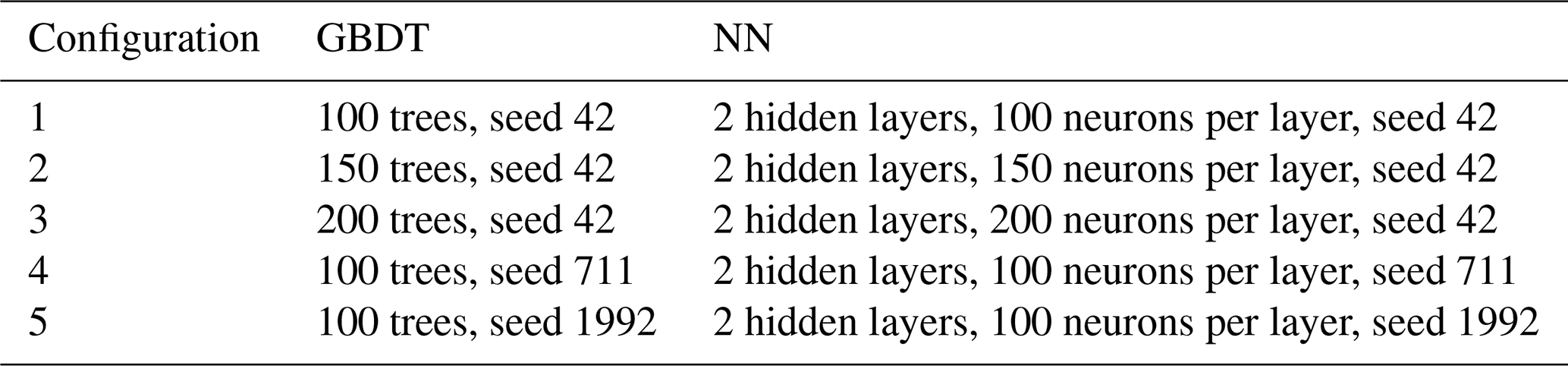
To evaluate the consistency of the ML metamodelling approach with GSA, two a priori assessments were performed: a sanity check of the bias–variance tradeoff for the important measures, and a convergence test for all sensitivity measures. Simply put, the bias–variance tradeoff establishes that increasing model flexibility produces smaller training error, but may lead to larger test error due to overfitting (e.g., James et al., 2023). In the present context, however, the objective was not to generalize to unseen data, but to accurately emulate the true model response. As discussed in Sect. 2.4, ${\widehat{\mathrm{PVI}}}_{\mathrm{i}}$ can provide a reliable approximation of T_i only if the metamodel is able to adequately reproduce the behaviour of the original model. From this perspective, a low training error was a necessary condition, and configurations that would be otherwise regarded as overfitting could be acceptable provided that they do not affect the feature importance estimates. Based on this, ${\widehat{\mathrm{PVI}}}_{\mathrm{i}}$ and mean |SHAP_i| were calculated for the GBDT and the NN metamodels using five overfitting configurations, as reported in Table 2. For the subsequent analysis, the less complex configuration was selected in each case, as it provided feature importance estimates comparable to the more complex configurations while achieving similar predictive performance.

Table 2 GBDT and NN metamodel configurations used during the sanity check. Configurations differ in model complexity and random initialization.

The convergence test was performed to verify that the sensitivity measures stabilized as the number of Monte Carlo samples increased. The test was carried out using a random subsampling strategy. Each subsample was drawn as an independent random sample without replacement from the full set of Monte Carlo simulations, with subsample sizes incremented in steps of 100 up to the full set of 10,000 samples, resulting in 100 subsampling matrices. For each subsampling matrix, ${\widehat{T}}_{\mathrm{i}}$, ${\widehat{\mathrm{PVI}}}_{\mathrm{i}}$, mean |SHAP_i|, and ${\widehat{\mathit{\beta }}}_{\mathrm{i}}^{\mathrm{2}}$ were computed, and convergence was assessed by comparing their values between consecutive subsample sizes. Sensitivity estimates corresponding to each subsampling matrix were normalized by dividing by the sum of all sensitivities. The Euclidean distance between the resulting sensitivity vectors at consecutive subsample sizes was then used as the convergence metric. This procedure ensured that the sensitivity results were robust with respect to the size of the training dataset. The purpose of this test was to verify that the full set of 10 000 samples was sufficient for the sensitivity estimates to stabilize, rather than to identify an exact sample size at which convergence was achieved. Since the subsamples were drawn from the same finite pool, consecutive draws of increasing size inevitably share some samples, leading to smoother variations as the subsample size approaches the full set. Despite this overlap, the test provided a reliable assessment of the stability of the sensitivity estimates across the range of subsample sizes considered.

4 Results and discussion

For clarity of presentation, the results for the Garlitz catchment are used as the guiding thread in this section. Corresponding figures for the Schackendorf and Augaard catchments are provided in the Supplementary Material. All three catchments exhibit consistent patterns, and their joint analysis is intended to ensure the robustness of the results rather than to highlight site-specific differences.

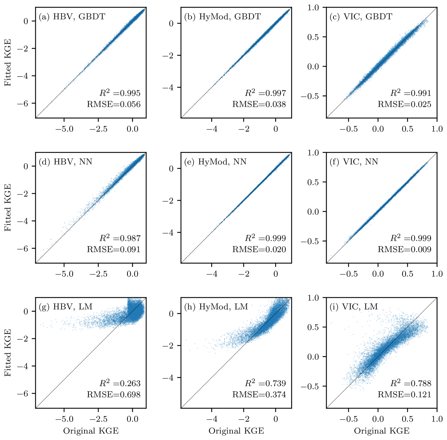
Figure 1 Predictive performance of the GBDT, NN, and LM metamodels for the three hydrologic models. GBDT and NN results are shown for configuration 1 (see Table 2). Scatter plots compare fitted and original KGE values for (a–c) GBDT, (d–f) NN, and (g–i) LM applied to HBV, HyMod, and VIC, respectively. The solid line indicates the 1:1 relationship. Coefficients of determination (R²) and root mean square errors (RMSE) are reported in each panel.

4.1 Sanity check and convergence test

Figure 1 summarizes the predictive performance of the GBDT, NN, and LM metamodels by comparing fitted and original KGE values across the three hydrologic models. For GBDT and NN, only configuration 1 is shown (see Table 2), as all five configurations exhibit similar predictive performance. Both GBDT and NN closely match the reference simulations for all three hydrologic models, indicating that they capture the dominant structure of the parameter–output relationship. The high R² values are expected, as the metamodels are evaluated on the same points used for training. This confirms that the surrogates adequately capture the behaviour of the original models, which is a necessary condition for the validity of Eq. (8) (see Sect. 2.4). In contrast, LM exhibits markedly weaker performance, particularly for HBV, with HyMod and VIC showing the highest linear response. The suitability and limitations of using an LM metamodel in contrast to GBDT and NN are discussed in the next section.

Figure 2 shows the sensitivity estimates obtained for the GBDT and NN metamodels across five flexible configurations, using both ${\widehat{\mathrm{PVI}}}_{\mathrm{i}}$ and mean |SHAP_i|. All five configurations correspond to deliberately overfitted metamodels (see Table 2), with coefficients of determination exceeding R²>0.98 for all hydrologic models. The importance curves corresponding to the different configurations largely overlap, indicating that the magnitude of the importance estimates remains remarkably consistent across varying model complexity and random initialization. In addition, panel titles in Fig. 2 report the mean ± standard deviation of pairwise Kendall τ and Spearman ρ between the importance vectors of the five configurations, which consistently show high values across all model–metamodel–importance combinations. This behaviour is observed for both ${\widehat{\mathrm{PVI}}}_{\mathrm{i}}$ and mean |SHAP_i|, suggesting that potential overfitting does not affect the resulting importance estimates. For a given importance measure, GBDT and NN exhibit nearly identical magnitudes and rankings, highlighting the robustness of the results with respect to the choice of metamodel. When comparing ${\widehat{\mathrm{PVI}}}_{\mathrm{i}}$ and mean |SHAP_i|, the relative ranking of influential parameters is generally preserved, while small differences in magnitude are observed. These differences are expected given the distinct theoretical foundations of the two approaches, but their close agreement indicates a consistent identification of dominant parameters across methods. Based on these results, configuration 1 was selected for GBDT and NN for the subsequent analysis, as it is the least complex while providing feature importance estimates comparable to the more complex configurations (see Sect. 3.5).

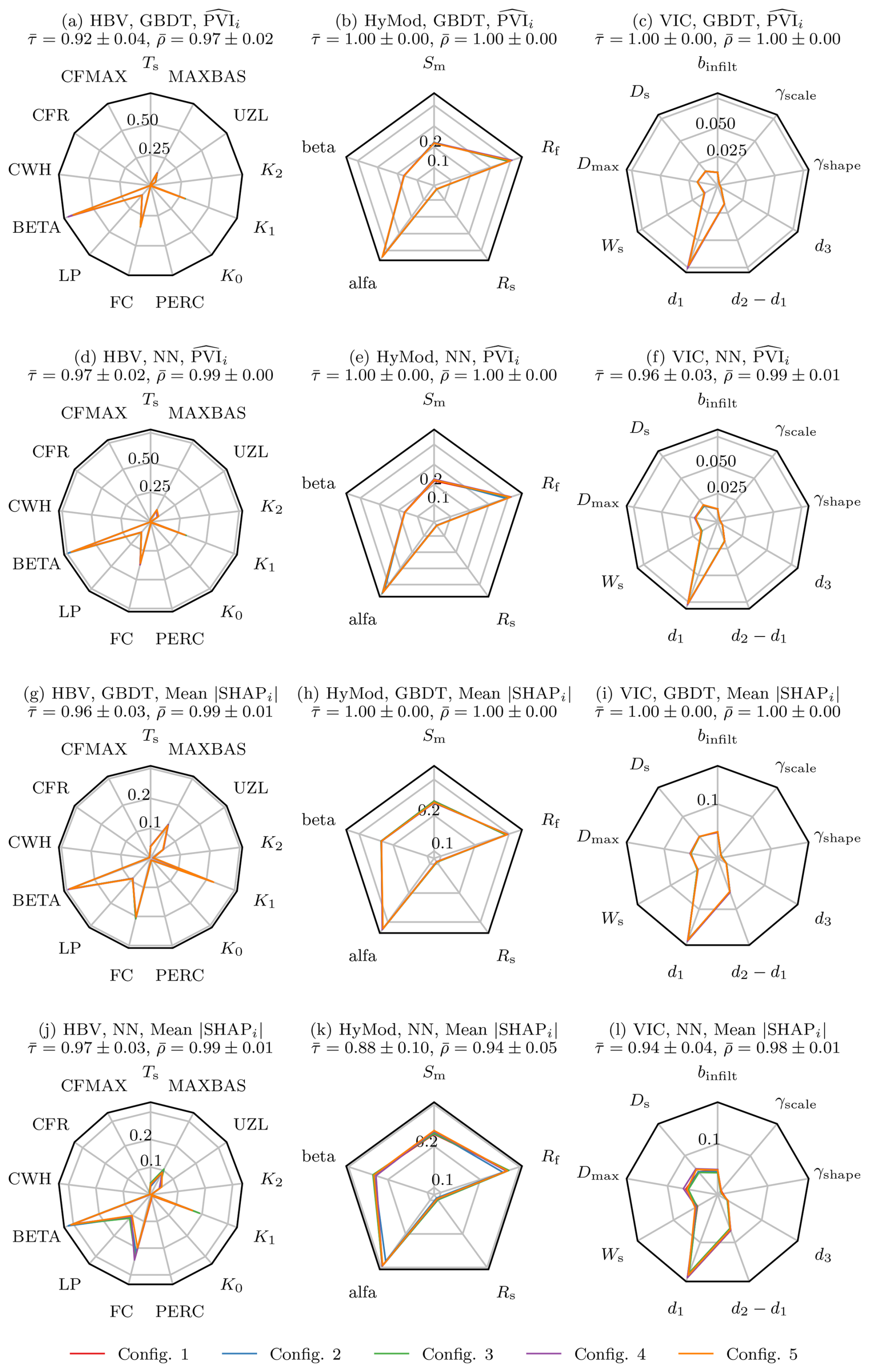
Figure 2 Sanity check of feature importance estimates for GBDT and NN metamodels across five overfitting configurations (see Table 2). Panels (a)–(c) show ${\widehat{\mathrm{PVI}}}_{\mathrm{i}}$ and panels (g)–(i) show mean |SHAP_i| for the GBDT metamodel applied to HBV, HyMod, and VIC, respectively, while panels (d)–(f) and (j)–(l) show the corresponding results for the NN metamodel. Each coloured line represents a different model configuration. Panel titles report the mean ± standard deviation of pairwise Kendall τ and Spearman ρ correlation between the importance vectors of the five configurations. The strong overlap of importance curves across configurations, supported by high $\stackrel{\mathrm{‾}}{\mathit{\tau }}$ and $\stackrel{\mathrm{‾}}{\mathit{\rho }}$ estimates, indicates that the feature importance estimates are robust to overfitting.

Finally, Fig. 3 presents the convergence behaviour of all sensitivity measures as a function of the number of Monte Carlo samples during the subsampling experiment. For all three hydrologic models, ${\widehat{T}}_{\mathrm{i}}$ exhibits stable and monotonic convergence as the subsample size increases. A similar convergence pattern is observed for ${\widehat{\mathrm{PVI}}}_{\mathrm{i}}$ and mean |SHAP_i| derived from the ML metamodels, indicating that the importance estimates stabilize with increasing training data. For all sensitivity measures, stabilization occurs at subsample sizes well below the full set of 10 000 samples, confirming that the number of Monte Carlo simulations used in this study was sufficient. Convergence is generally faster and smoother for HyMod and VIC, whereas HBV shows comparatively slower convergence and higher variability across sensitivity measures. This behaviour is consistent with the higher structural complexity of HBV, which involves 13 parameters, compared to the more parsimonious HyMod (5 parameters) and VIC (9 parameters), and reflects the increased sampling requirements associated with higher-dimensional parameter spaces. In addition, mean |SHAP_i| values computed from the GBDT metamodel display slightly reduced stability for HBV relative to the other cases.

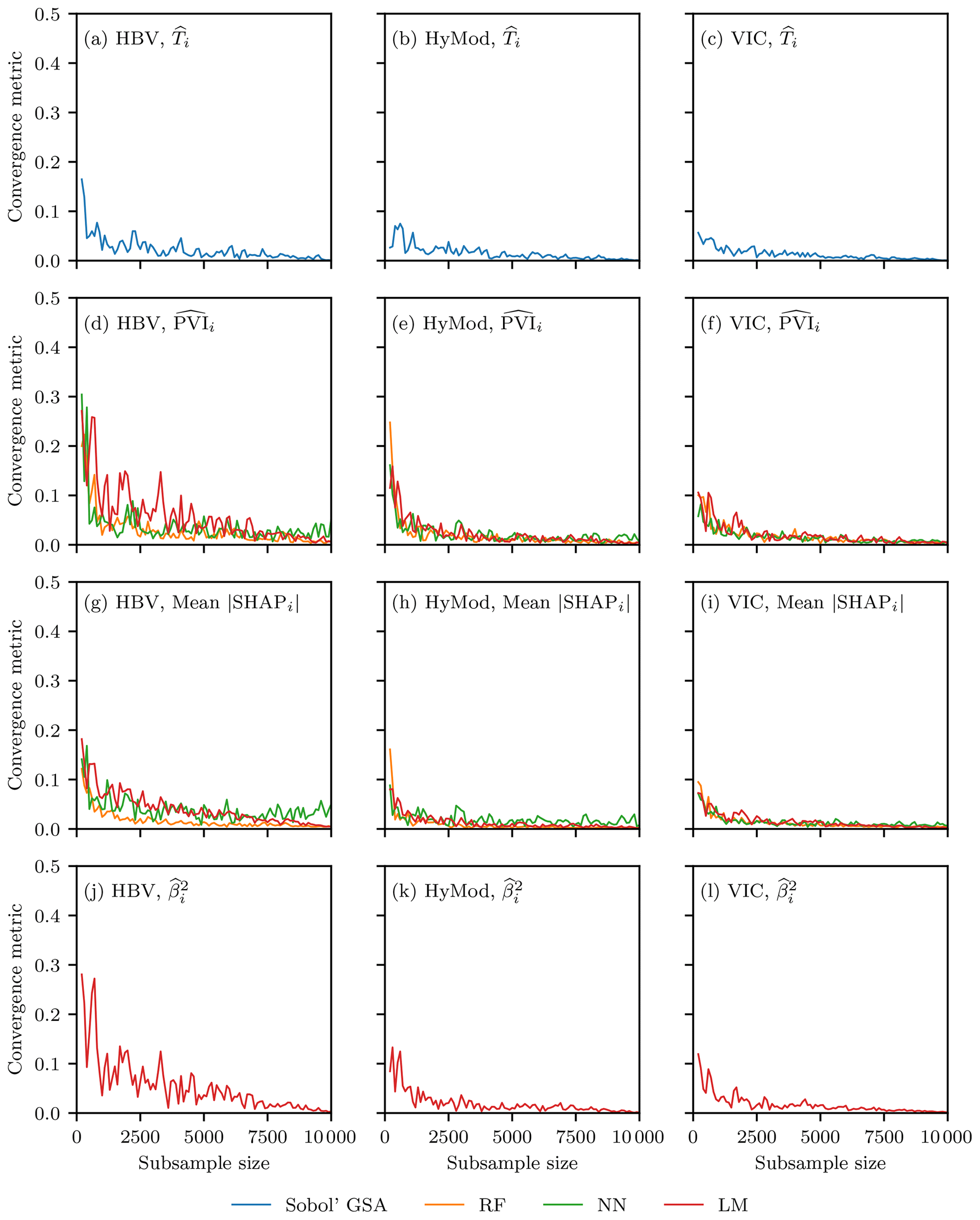
Figure 3 Convergence of sensitivity measures as a function of subsample size. Panels (a)–(c) show the convergence of ${\widehat{T}}_{\mathrm{i}}$, panels (d)–(f) of ${\widehat{\mathrm{PVI}}}_{\mathrm{i}}$, panels (g)–(i) of mean |SHAP_i|, and panels (j)–(l) of ${\widehat{\mathit{\beta }}}_{\mathrm{i}}^{\mathrm{2}}$ for HBV, HyMod, and VIC, respectively. The convergence metric is computed as the Euclidean distance between normalized sensitivity vectors obtained from consecutive subsample sizes. Normalization was performed by dividing by the sum of all sensitivities.

4.2 Relationship between T_i and PVI_i

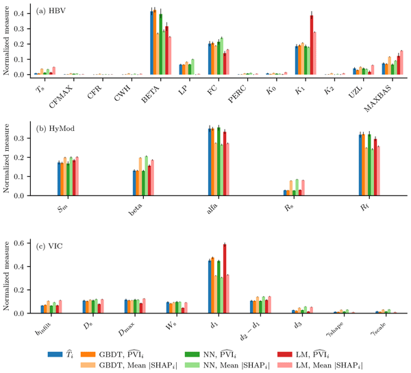
The theoretical relationship between T_i and PVI_i expressed in Eq. (8) was examined empirically for the HBV, HyMod, and VIC models using the importance measures derived from GBDT, NN, and LM metamodels. Figure 4 shows the normalized ${\widehat{T}}_{\mathrm{i}}$ together with normalized ${\widehat{\mathrm{PVI}}}_{\mathrm{i}}$ estimates and normalized mean |SHAP_i| values obtained from the three metamodels. As in the convergence analysis (Fig. 3), values were normalized by dividing by the sum of all sensitivities in order to facilitate a direct comparison and produce a consistent ranking of parameters. For the GBDT and NN metamodels, ${\widehat{\mathrm{PVI}}}_{\mathrm{i}}$ reproduces both the ranking and the relative magnitude of ${\widehat{T}}_{\mathrm{i}}$ across all three hydrologic models, reflecting only minor discrepancies. In contrast, LM-based ${\widehat{\mathrm{PVI}}}_{\mathrm{i}}$ provides a good approximation of ${\widehat{T}}_{\mathrm{i}}$ for HyMod and VIC, but exhibits larger deviations for HBV, particularly in the relative importance assigned to dominant parameters. This behaviour is consistent with the comparatively poor predictive performance of the LM for HBV (Fig. 1). This expected limited fit of the LM underscores that the ability of ${\widehat{\mathrm{PVI}}}_{\mathrm{i}}$ to approximate ${\widehat{T}}_{\mathrm{i}}$ depends critically on the accuracy with which the metamodel captures the underlying model response.

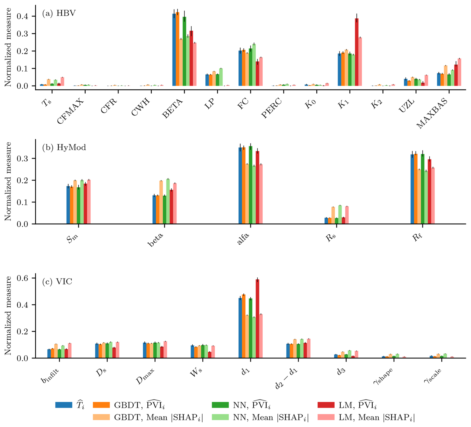
Figure 4 Parameter rankings for (a) HBV, (b) HyMod, and (c) VIC. Bars show normalized ${\widehat{T}}_{\mathrm{i}}$ from variance-based GSA, normalized ${\widehat{\mathrm{PVI}}}_{\mathrm{i}}$ estimates, and normalized mean $\left|{\mathrm{SHAP}}_{\mathrm{i}}\right|$ with ${\widehat{T}}_{\mathrm{i}}$ obtained from GBDT, NN, and LM metamodels. Sensitivity measures were normalized by dividing each by the sum of all sensitivities, as in the convergence test. Thin black lines indicate 95 % confidence intervals.

The correspondence between ${\widehat{T}}_{\mathrm{i}}$ and ${\widehat{\mathrm{PVI}}}_{\mathrm{i}}$ is further illustrated in Fig. 5 (panels a–c), which directly compares the two quantities for each hydrologic model parameter and metamodel. GBDT- and NN-based estimates closely follow the theoretical relationship, providing clear numerical support for the connection established in Eq. (8). For the LM, agreement with the theoretical relationship is observed only for HyMod, whereas a weaker correspondence is observed for HBV and VIC – in line with how well the LM is able to capture hydrologic model behaviour. The close agreement observed between ${\widehat{T}}_{\mathrm{i}}$ and ${\widehat{\mathrm{PVI}}}_{\mathrm{i}}$ for GBDT is in line with previous theoretical and numerical results under independence assumptions (Wei et al., 2015; Antoniadis et al., 2021). While earlier work primarily focused on random forest, the present results extend these findings by demonstrating that alternative ML metamodels can also provide reliable approximations of ${\widehat{T}}_{\mathrm{i}}$, provided that they accurately reproduce the underlying input–output relationship. In particular, the strong performance of the NN metamodel, and the satisfactory behaviour of the LM for HyMod, indicate that the validity of ${\widehat{\mathrm{PVI}}}_{\mathrm{i}}$-based sensitivity estimates is not tied to a specific algorithm, but rather to the fidelity of the regression surrogate. This observation corroborates the insight of Gregorutti et al. (2017), who emphasized that the empirical estimation of PVI_i strongly depends on the algorithm used to approximate the regression function. In contrast, Rouzies et al. (2023) reported that the relationship between ${\widehat{\mathrm{PVI}}}_{\mathrm{i}}$ and ${\widehat{T}}_{\mathrm{i}}$ was not well respected when using a random forest surrogate for a distributed, physically based pesticide transfer model with 145 input parameters, and after applying a screening procedure to reduce the dimension of the problem. In their study, the poor predictive performance of the surrogate was identified as the likely cause, further underscoring that the practical applicability of Eq. (8) depends on surrogate fidelity. It should be noted, however, that in our work all three models were used in lumped configurations: HBV and HyMod are lumped conceptual rainfall-runoff models, while VIC, though a land-surface model with a more complex parameterization including surface and energy balance components, was likewise run in a lumped setup. This limits the degree of structural complexity relative to fully distributed applications such as that of Rouzies et al. (2023), and may partly explain why high surrogate fidelity was more readily achieved in our study.

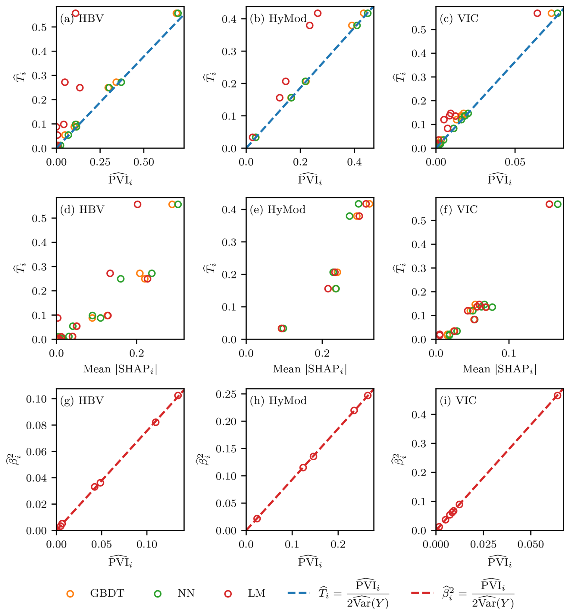
Figure 5 Comparison of different sensitivity estimates across hydrologic models. Panels (a)–(c) compare ${\widehat{\mathrm{PVI}}}_{\mathrm{i}}$ with ${\widehat{T}}_{\mathrm{i}}$ for HBV, HyMod, and VIC, respectively. Panels (d)–(f) compare mean $\left|{\mathrm{SHAP}}_{\mathrm{i}}\right|$ with ${\widehat{T}}_{\mathrm{i}}$, and panels (g)–(i) compare ${\widehat{\mathrm{PVI}}}_{\mathrm{i}}$ with ${\widehat{\mathit{\beta }}}_{\mathrm{i}}^{\mathrm{2}}$ for the LM metamodel. Dashed lines indicate the corresponding theoretical relationships. Colours denote the ML metamodel used.

In recent hydrologic studies, tree-based ensemble approaches and feature importance measures have been widely used as exploratory tools to analyse large-sample datasets and to identify dominant drivers of hydrologic behaviour, for example, in the context of intercatchment groundwater flow (Liu et al., 2020), hydrologic signatures (Addor et al., 2018), and flood-generating processes (Stein et al., 2021). In these applications, different XAI approaches are used to help elucidate empirical relationships learned by a random forest. ML metamodels are also efficient alternatives to complex hydrologic models, such as VIC (Gu et al., 2020; Sun et al., 2023) and ParFlow.CLM (Lim and Wang, 2022), and have already been applied to accelerate studies on climate impacts (Schnorbus and Cannon, 2014) as well as for regionalization and calibration of conceptual hydrologic models (Farahani et al., 2025; Tang et al., 2025). A closer connection to sensitivity analysis is found in the work of Brêda et al. (2024), who employed feature importance as a diagnostic approach for global hydrologic and land-surface models using a random forest surrogate. The present study builds directly on this emerging line of research by explicitly linking feature importance measures to variance-based total-effect sensitivity indices across multiple hydrologic models and metamodel classes.

4.3 Alternative approaches to estimate sensitivities

As an alternative to ${\widehat{\mathrm{PVI}}}_{\mathrm{i}}$, Fig. 5 also examines the possibility of using mean |SHAP_i| and ${\widehat{\mathit{\beta }}}_{\mathrm{i}}^{\mathrm{2}}$ for GSA. The normalized mean |SHAP_i| values included in Fig. 4 further illustrate this comparison at the parameter level. Panels (d)–(f) of Fig. 5 contrast mean |SHAP_i| with ${\widehat{T}}_{\mathrm{i}}$, revealing a clear monotonic relationship across all hydrologic models, with larger dispersion than ${\widehat{\mathrm{PVI}}}_{\mathrm{i}}$ (panels a–c). Results obtained with GBDT and NN are very similar for all hydrologic models, whereas, as observed for ${\widehat{\mathrm{PVI}}}_{\mathrm{i}}$, LM-based results are satisfactory for HyMod and VIC, where the model response exhibits a stronger degree of linearity. Despite the increased dispersion, mean |SHAP_i| preserves nearly the same ranking of influential parameters as identified by ${\widehat{\mathrm{PVI}}}_{\mathrm{i}}$ and ${\widehat{T}}_{\mathrm{i}}$. Panels (g)–(i) compare ${\widehat{\mathrm{PVI}}}_{\mathrm{i}}$ with ${\widehat{\mathit{\beta }}}_{\mathrm{i}}^{\mathrm{2}}$ for the LM metamodel, confirming the proportionality between the two measures established in Eq. (14).

Beyond providing a global ranking, SHAP_i values enable a more detailed and informative sensitivity analysis across both the parameter space and the target variable space, as illustrated in Fig. 6 for HyMod using the GBDT metamodel. Panel (a) reports a global importance ranking based on mean |SHAP_i|, which coincides with the results shown in Fig. 5 (panel e). Panel (b) shows the distribution of SHAP_i values across the parameter space, highlighting that parameters with similar global importance can exhibit markedly different local contributions depending on their values (e.g., S_m and beta). Panel (c) focuses on the most influential parameter, alfa, illustrating how its contribution to the model response varies across its range. Finally, panel (d) displays SHAP_i values for alfa as a function of KGE, showing that the region of highest model performance (i.e., larger KGE values) is associated with positive and comparatively larger SHAP_i values for alfa.

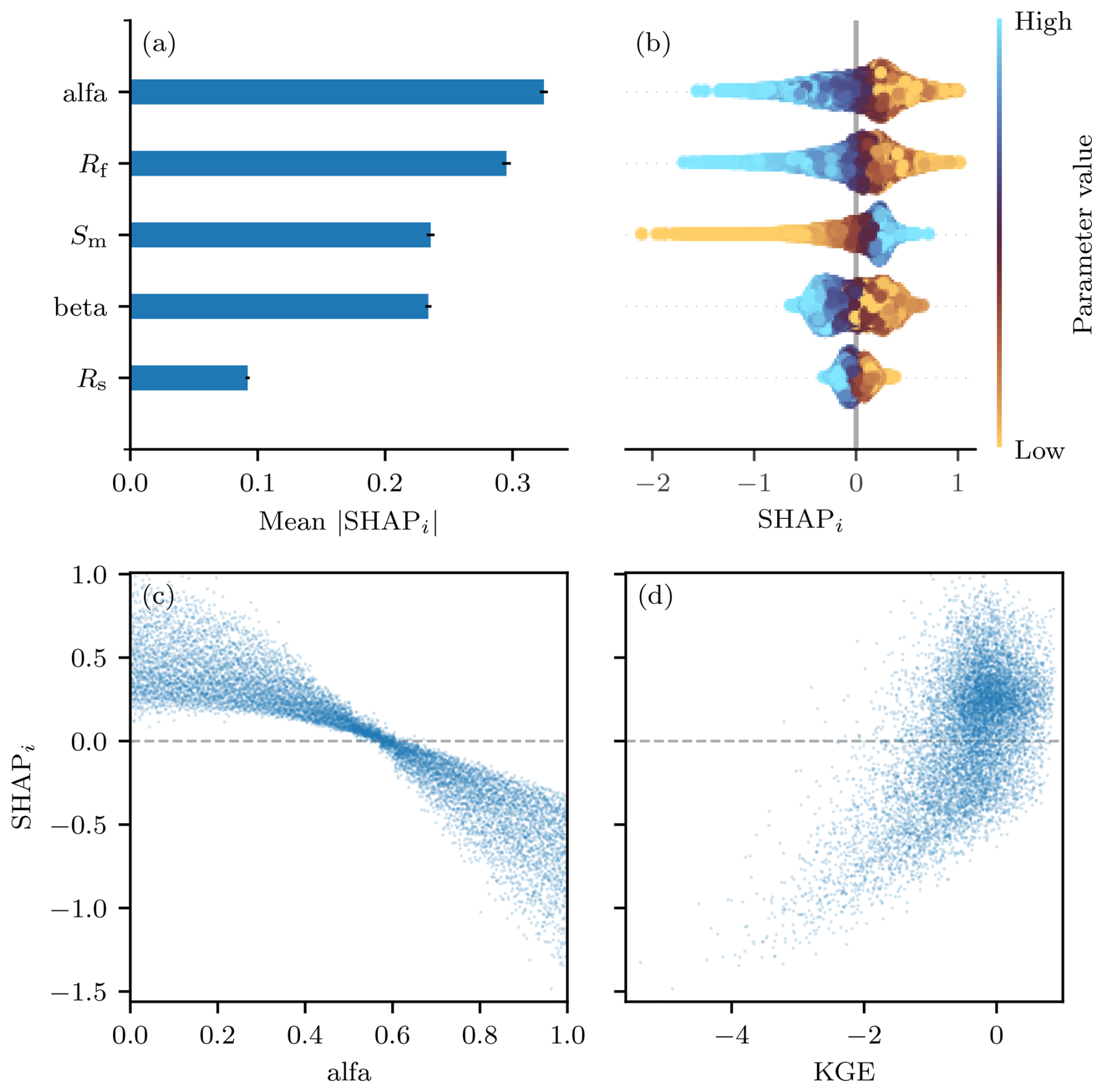
Figure 6 Detailed SHAP_i-based sensitivity analysis for HyMod using the GBDT metamodel. Panel (a) shows the global parameter ranking based on mean |SHAP_i|, with thin black lines indicating 95 % confidence intervals. Panel (b) displays the distribution of SHAP_i values across the parameter space, coloured by parameter value. Panel (c) illustrates the variation of SHAP_i for the most influential parameter, alfa, across its range. Panel (d) shows SHAP_i values for alfa as a function of KGE, highlighting how parameter contributions vary across model performance levels.

The ability of SHAP_i values to characterize how parameter influence varies across both the parameter space and the target variable space is conceptually closely related to the Distributed Evaluation of Local Sensitivity Analysis (DELSA) introduced by Rakovec et al. (2014). DELSA was developed to move beyond single summary measures of sensitivity by providing distributions of parameter sensitivities across the parameter space, thereby revealing regimes in which parameters may alternate between being influential or negligible. As emphasized by Rakovec et al. (2014), the ability to understand how parameter sensitivities vary throughout parameter space is critical for informing decisions related to data collection and model development, particularly when sensitivities are evaluated with respect to performance metrics. This perspective aligns with the broader critique of GSA articulated by Razavi and Gupta (2015, 2016), who demonstrated that global aggregation can obscure important behaviour when sensitivity is assessed using performance metrics. The SHAP_i-based analyses presented here address these limitations by providing sample-specific contributions that can be examined jointly in parameter space and target variable space.

In this sense, SHAP_i values provide a complementary perspective to distributed sensitivity approaches such as DELSA, while naturally integrating with ML metamodelling frameworks. It is important to emphasize that neither SHAP_i nor DELSA should be regarded as equivalent to classical GSA measures such as ${\widehat{T}}_{\mathrm{i}}$. DELSA is a hybrid local-global approach that provides distributions of parameter sensitivities across the parameter space, rather than the single summary measures characteristic of GSA (see also Dell'Oca et al., 2020, for a non-aggregated approach based on copula density-driven metrics). Similarly, SHAP_i operates as a local prediction-explanation method that attributes the contribution of each input to individual predictions, and the global importance derived from mean absolute SHAP_i values is an aggregation of these local explanations rather than a variance decomposition index. This complementary relationship between SHAP and SA-based approaches has been explored in recent studies. Panigrahi et al. (2025) compared an SA-based explainer, the Explainer Variogram Analysis of Response Surface (XVARS), with SHAP, showing that both approaches mostly align in their feature rankings. However, they differ in that XVARS characterizes the entire response surface of ML models, whereas SHAP provides local explanations that are generalized by averaging over sampled data points and may miss behaviour in regions without training data. Panigrahi et al. (2026) extended this comparison, finding that XVARS and SHAP are broadly consistent in identifying dominant features but differ in scope and robustness: SA-based methods are independent of training sample size and more robust to sampling variability, whereas SHAP scales linearly with sample size and its importance estimates depend on the underlying ML architecture.

Last, despite the absence of a formal link between SHAP_i and ${\widehat{T}}_{\mathrm{i}}$, both measures share a common theoretical root in the Shapley value framework from cooperative game theory, which provides a principled approach for allocating contributions among interacting variables. In the context of GSA, the same principle has been adopted through Shapley effects, which allocate contributions to the variance of model outputs among input variables. Owen (2014) demonstrated that, for independent inputs, Shapley effects are bounded by the first-order and total-effect Sobol indices. Although SHAP and Shapley effects address different attribution problems, both rely on the same theoretical foundation. Hence, when SHAP values are aggregated over a representative sample of the input space, as in the mean |SHAP_i| values used in this work, they provide a global measure of variable influence that, while not equivalent to Sobol indices or Shapley effects, can be considered a complementary global sensitivity measure.

5 Conclusions

This technical note examined the practical relationship between GSA and ML metamodelling within a hydrologic modelling context. Using three hydrologic models (HBV, HyMod, and VIC) applied over three catchments in Germany, and taking KGE as the target variable, we computed Sobol' T_i and assessed whether GBDT, NN, and LM metamodels can reproduce these sensitivities through two feature importance measures, namely PVI_i and SHAP_i values.

The numerical experiments provided clear empirical evidence supporting the theoretical relationship between T_i and PVI_i underlying Eq. (8). Across all hydrologic models, the GBDT and NN metamodels reproduced both the ranking and the relative magnitude of T_i using PVI_i, with only minor discrepancies. The results further showed that, as expected, the reliability of PVI_i as a proxy for T_i depends critically on metamodel performance: when the LM failed to accurately reproduce the hydrologic model response, agreement between PVI_i and T_i deteriorated, whereas satisfactory performance and agreement were obtained for the more linear case.

Alternative sensitivity measures derived from ML metamodels were also assessed. Mean |SHAP_i| exhibited a consistent monotonic relationship with T_i and preserved nearly the same ranking of influential parameters observed for T_i and PVI_i. For the LM, ${\mathit{\beta }}_{\mathrm{i}}^{\mathrm{2}}$ was proportional to PVI_i, as expected from Eq. (14). Importantly, SHAP_i values provided additional diagnostic insight by enabling a distributed evaluation of parameter sensitivities across both the parameter space and the model output space, thereby revealing important effects that are averaged out by single summary measures of sensitivity.

The results also highlight the key computational motivation for using ML metamodelling for GSA. Classical variance-based estimation of ${\widehat{T}}_{\mathrm{i}}$ requires n(p+2) model evaluations, which can be prohibitive for complex or high-dimensional models. In contrast, once a surrogate model is trained, ${\widehat{\mathrm{PVI}}}_{\mathrm{i}}$ can be computed at negligible additional cost, while relying only on the n model evaluations used for training. This makes ML metamodels particularly attractive for efficient sensitivity analysis of computationally demanding models.

From a hydrologic modelling perspective, these findings support ML metamodelling as a practical and flexible framework for GSA, with direct relevance for parameter prioritization, model diagnosis, and the interpretation of model behaviour across model performance levels. By establishing a clear and empirically validated link between variance-based sensitivity indices and ML-based feature importance measures, this work helps bridge methodological developments in GSA and XAI with applied hydrologic modelling practice. The analysis was conducted for catchments characterized by semi-humid climatic conditions and predominantly groundwater-driven runoff generation, which may influence the generality of the results. Future research could extend this analysis to catchments with contrasting hydroclimatic and physiographic characteristics, to settings with dependent inputs, alternative model outputs of interest, and more complex hydrologic modelling configurations, as well as to applications where metamodels are used beyond sensitivity estimation, such as for exploring uncertainties, supporting calibration, or transferring across catchments.

Appendix A: Mathematical definition of SHAP values

Let Y=f(X) be the deterministic model defined in Sect. 2.1, and let $x=(x_{\mathrm{1}},\mathrm{\dots },x_p)$ be a specific realization of the input vector X. The SHAP value of the ith input variable for the prediction f(x) is defined as the Shapley value of the conditional expectation function (Lundberg and Lee, 2017):

$$\begin{array}{}\text{(A1)}& \begin{array}{rl}{\mathit{\varphi }}_{\mathrm{i}}(f,x)& =\sum _{S\subseteq P\setminus \mathit{\left\{}i\mathit{\right\}}}{\displaystyle \frac{\left|S\right|\mathrm{!}(p-|S|-\mathrm{1})\mathrm{!}}{p\mathrm{!}}}\\ & [\mathbb{E}\left[f\left(\mathit{X}\right)|{\mathit{X}}_{S\cup \mathit{\left\{}i\mathit{\right\}}}=x_{S\cup \mathit{\left\{}i\mathit{\right\}}}\right]\\ & -\mathbb{E}\left[f\left(\mathit{X}\right)|{\mathit{X}}_S=x_S\right]]\end{array}\end{array}$$

where $P=\mathit{\{}\mathrm{1},\mathrm{\dots },p\mathit{\}}$ is the set of input indices and the sum runs over all subsets S of P that exclude i.

The two conditional expectations represent the expected model output when only a subset of inputs is known:

• $\mathbb{E}\left[f\right(\mathit{X}\left)\right|{\mathit{X}}_{S\cup \mathit{\left\{}i\mathit{\right\}}}=x_{S\cup \mathit{\left\{}i\mathit{\right\}}}]$ is the expected model output when the inputs in S and X_i are set to their values in x, while the remaining inputs vary according to their prescribed distributions.

• $\mathbb{E}\left[f\right(\mathit{X}\left)\right|{\mathit{X}}_S=x_S]$ is the same expectation, but now X_i is left unknown and marginalized over its distribution.

Their difference measures the change in expected model output when X_i is made known. This difference depends on which other inputs are already known, so the Shapley value averages this difference over all possible subsets S that exclude i. The weight $\left|S\right|\mathrm{!}(p-|S|-\mathrm{1})\mathrm{!}/p\mathrm{!}$ gives each subset S its appropriate share according to cooperative game theory (Shapley, 1953), ensuring that the contribution of each input is fairly allocated regardless of the order in which inputs are considered.

The exact computation of SHAP values is challenging (Lundberg and Lee, 2017). In practice, SHAP values are approximated using estimators that exploit the structure of the prediction model, such as TreeExplainer for tree-based models or DeepExplainer for neural networks. This computational challenge also motivates the use of ML metamodels $\widehat{f}$ as efficient surrogates of the original model f, for which SHAP values can be computed much more efficiently.

Throughout this paper, the ϕ_i values obtained from a ML metamodel $\widehat{f}$ are referred to as SHAP_i, and their absolute values averaged over all samples yield the mean |SHAP_i|, which is used here as a global measure of parameter importance.