Integrating a global glacier model into local hydrological modeling: Impacts on melt contributions

Snow and glacier meltwater are critical water resources for mountain regions, yet their accurate representation in hydrological models remains challenging. As climate change alters the timing and magnitude of melt contributions, accurate partitioning between snow and glacier sources becomes increasingly important. To address this challenge, this study couples the hydrological model HBV (as implemented in the Raven modeling framework) with the Global Glacier Evolution Model GloGEM and integrates a snow redistribution scheme for application across 14 glaciated headwater catchments in Switzerland. At this local catchment scale, we investigate whether glacier constraints and the addition of snow redistribution reduce parameter equifinality and increase the reliability of melt contribution estimates. Simulations are evaluated against observed streamflow, gridded snow water equivalent data, and glacier melt data based on observed mass balance. The gravitational snow redistribution algorithm successfully prevents unrealistic high-elevation snow accumulation and improves catchment average SWE simulation performance. Uncoupled HBV configurations outperform coupled HBV-GloGEM setups according to streamflow metrics. However, this superior performance is achieved by simulating glacier melt rates exceeding GloGEM estimates and glacier storage change data by factors of 2–3 in some catchments, effectively using glacier ice to offset precipitation biases in forcing data, which can be critical for climate change impact studies. Within a single model configuration, glacier melt contributions can vary by more than a factor of three among the best-performing parameter sets, and by up to an order of magnitude in weakly glacierized catchments, highlighting severe parameter equifinality. Coupling the HBV model with GloGEM (calibrated using glacier-specific geodetic mass balance) produces glacier melt consistent with observations and substantially improves identifiability of both glacier and snowmelt contributions. Despite lower streamflow performance metrics, glacier melt constraints prevent compensatory errors that would compromise projections as melt dynamics shift under climate change. Applying this framework to future climate scenarios and integrating additional constraints such as snow observations may further improve the reliability of melt contribution projections.

1 Introduction

Many mountainous and high-latitude regions around the globe receive the majority of their annual precipitation as snow and rely on snow and glacier meltwater for agriculture and human consumption (Kaser et al., 2010; Mankin et al., 2015; Huss and Hock, 2018; Viviroli et al., 2020). This highlights the importance of the cryosphere as temporary water storage, reducing interannual streamflow variability by accumulating precipitation during cold and wet seasons and releasing it during warm and dry periods (Jansson et al., 2003; Viviroli et al., 2011). This delayed release helps mitigate extreme water shortages on seasonal and longer time scales, sustaining downstream water supply for regional ecosystems, groundwater recharge, human consumption, irrigation, and hydropower (Freudiger et al., 2017; Biemans et al., 2019; van Tiel et al., 2020). It is therefore essential to understand the impact of climate change on the cryosphere and river streamflow for sustainable water management of future water resources (Molden et al., 2017).

Rising global temperatures are expected to reduce the water storage capacity of both glaciers and snowpack, which will have major consequences for the downstream water supply (Immerzeel et al., 2020). As both the fraction and frequency of snowfall are declining (Frei et al., 2018), the extent of snow-covered areas in the Alps is decreasing (Sturm et al., 2017; Hanzer et al., 2018). Consequently, the snow cover season in mountain regions is projected to shorten, with a delayed onset of snow cover and an earlier onset of snow melting, leading to a shift of the peak melting season towards earlier periods (Arnoux et al., 2021). Most glaciers have lost and continue to lose a substantial part of their volume and area (Hugonnet et al., 2021). Farinotti et al. (2012) found a combined response to this glacier loss with first increasing and then decreasing annual streamflow depending on the glacier volume in the catchment, illustrating the “peak water” effect. As a result, snow- and ice-dominated catchments are expected to experience altered flow seasonality, with higher winter discharge and reduced summer runoff (Horton et al., 2006; Han et al., 2024), affecting water availability in downstream regions (Arnoux et al., 2021).

To predict these hydrological changes, it is essential to include an accurate representation of glacier and snowpack projections in hydrological models. A range of modeling approaches with varying complexity have been developed and applied in snow- and ice-dominated mountainous catchments (e.g., Hock, 2003; Hanzer et al., 2018; Immerzeel et al., 2020). Hydrological models often rely on temperature-index approaches to simulate snow accumulation and melt while neglecting snow redistribution processes. This can produce unrealistic snow accumulation patterns with excessive snow storage at high elevations known as “snow towers” (Freudiger et al., 2017). In reality, post-depositional processes such as wind-driven transport (Winstral et al., 2017; Reynolds et al., 2021) and avalanching (Bernhardt and Schulz, 2010) frequently remove snow from exposed areas, leaving summits, cliffs, and steep slopes largely snow-free (Freudiger et al., 2017). Ignoring these processes can therefore lead to local overestimation of snow water equivalent (SWE). Representing snow redistribution is thus essential for accurately simulating catchment-scale SWE and melt dynamics.

While incorporating snow redistribution improves the representation of snow processes, another important step toward more realistic hydrological modeling in high-elevation regions involves improving glacier dynamics. To this end, a few recent studies have coupled large-scale hydrological models with global glacier models (Wiersma et al., 2022; Hanus et al., 2024). Wiersma et al. (2022) found that coupling a global hydrological model with a global glacier model increases the performance to reproduce basin streamflow in highly glaciated catchments and prevents underestimation of glacier runoff. Hanus et al. (2024) found that improved glacier representation can prevent underestimations of future streamflow changes, even far downstream at the outlet of large glaciated river basins. Although these studies demonstrate the advantages of coupling hydrological models with global glacier models, such approaches have been developed primarily for large-scale basins with limited evaluation at the local catchment-scale (up to a few hundred km²). It remains unclear whether global glacier models provide comparable benefits when applied at these scales, particularly since small catchments may exhibit different sensitivities to glacier representation than large basins. In one of the few local-scale studies, Pesci et al. (2023) coupled the physically-based hydrological model WaSiM (Schulla and Jasper, 2007) with the Open Global Glacier Model (OGGM) (Maussion et al., 2019) in an Austrian headwater catchment and compared this approach to traditional volume-area scaling (Bahr et al., 1997) to simulate glacier evolution. Although both approaches produced similar results for streamflow during the historical period, they revealed substantial divergences in future projections, suggesting that the choice of glacier representation may have a limited impact on model performance during calibration but significant implications for long-term predictions.

Hydrological modeling remains an essential tool for understanding the hydrological behavior of glaciated catchments and projecting their response to climate change. However, these models often exhibit equifinality, where multiple parameter sets yield similarly good streamflow simulations, but represent underlying processes differently (Beven, 2006). For instance, Stahl et al. (2008) found that equally well-performing streamflow simulations corresponded to widely varying glacier mass balance estimates. This highlights that deficiencies in model input, structure, or parameterization can be compensated (Duethmann et al., 2015). Introducing process-based constraints through glacier model coupling, along with improved snow redistribution schemes, has the potential to reduce such ambiguities. Yet, how these additional constraints affect hydrological model calibration, parameter identifiability, and the quantification of seasonal snow and glacier melt contributions remains largely unexplored. Addressing these questions is key to improving confidence in model-based assessments of future water availability in mountain regions.

To address these challenges, we present, to our knowledge, the first integration of glacier runoff from a global glacier model into a conceptual hydrological model at the local scale. We combine the hydrological modeling framework Raven (Craig et al., 2020) with the global glacier model GloGEM (Huss and Hock, 2015) through a mass-conserving, model-agnostic coupling approach. In addition, we integrate a snow redistribution scheme (Bernhardt and Schulz, 2010) to prevent unrealistic high-elevation snow accumulation. Together, these components aim to improve the representation of cryospheric dynamics at the catchment scale. We apply this framework in a systematic multi-catchment assessment across 14 glaciated headwater catchments in Switzerland with a range of glacier coverage (3 %–60 %), allowing us to evaluate the transferability and limitations of the coupling approach. The simulation results are evaluated against observed streamflow, a gridded SWE product (Marty et al., 2025a), and annual glacier storage change data from Switzerland (van Tiel et al., 2026). Finally, we analyze how different model configurations influence calibrated parameter values and assess the resulting impacts on annual and seasonal snow and glacier melt contributions.

2 Study site

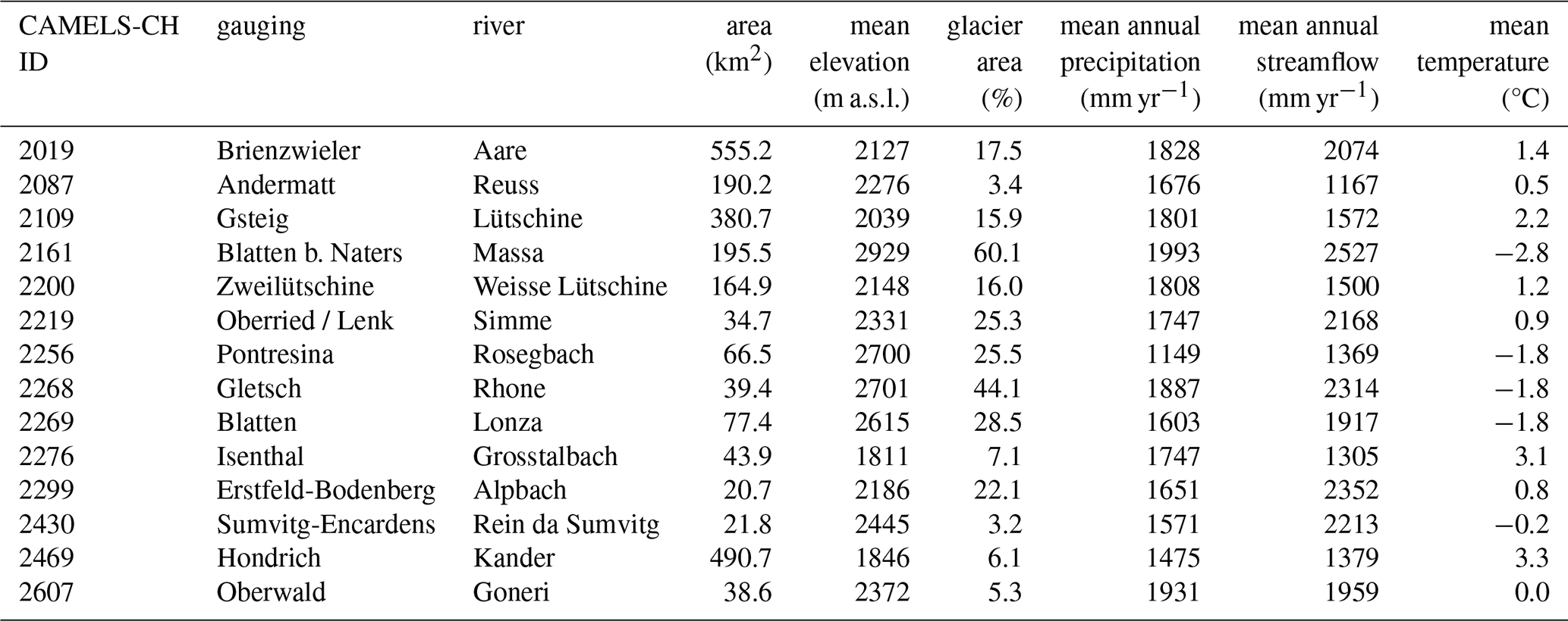
For this study, 14 glaciated catchments located in the Swiss Alps were selected (Fig. 1 and Table 1). This dataset corresponds to all Swiss gauged catchments with glacier cover but largely unaffected by hydropower infrastructure. Dominant land uses in these areas are alpine pastures, natural grasslands, forests, shrubs, water bodies, including lakes, glaciers, rock outcrops and rock debris from periglacial and paraglacial processes (Marsoner et al., 2023). The dominant geology in the catchments is granite and gneiss (Swisstopo – Swiss Federal Office of Topography, 2020). The selected catchments are mesoscale, with areas up to 555 km². They are located at high elevations, with mean catchment elevations ranging from 1811 to 2929 m a.s.l. (Table 1). Due to large elevation differences within individual catchments, strong vertical temperature and precipitation gradients are present. Their climate is characterized by low annual average temperatures ranging from −2.8 to 3.3 °C and a high mean annual precipitation ranging between 1149 and 1993 mm yr⁻¹ with a high fraction of precipitation falling as snow, ranging from 26 % in the Kander catchment (ID 2469) to 81 % in the Massa catchment (ID 2161). The Rosegbach catchment (ID 2256) is notably drier than the others since it is located more intra-Alpine. Snow typically covers much of the landscape between November and April, with snowfall possible year-round at higher elevations. The hydrological regimes of the catchments are either glacier-dominated or nival (snowmelt-driven), with peak streamflow occurring during the summer months due to snow and glacier melt (HADES, 2025). Glacier cover in the year 2000 varies substantially between catchments, ranging from 3.2 % in the Rein da Sumvitg catchment (ID 2430) to 60.1 % in the Massa catchment (ID 2161), according to the RGI v6.0 glacier outlines (RGI Consortium, 2017).

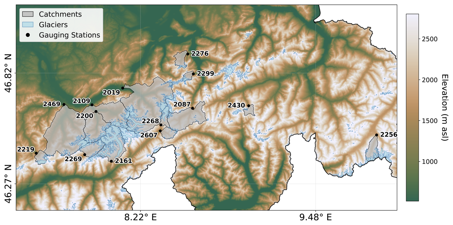
Figure 1 Map of study area in Switzerland with SwissTopo DEM (Swisstopo – Swiss Federal Office of Topography, 2020). Grey polygons show selected catchments with their CAMELS-CH ID and gauging station (black point), and light blue polygons the glaciated area according to RGI v6.0 with the reference year 2000.

Table 1 Overview of the selected catchments. Reference period for mean annual temperature, precipitation and streamflow: 2000–2021 (MeteoSwiss, 2013). Reference year for relative glacier area: 2000 (RGI Consortium, 2017).

3 Methodology

An automated workflow was developed to set up the hydrological model for all catchments of interest in Switzerland. The required input datasets and model components are described in Sect. 3.1 and 3.2. The workflow automatically generates inputs for the hydrological model, calibrates the model, and runs simulations for each catchment, as described in Sect. 3.3 to 3.5.

3.1 Data

CAMELS-CH (Catchment Attributes and Meteorology for Large-sample Studies – Switzerland) is an open large-sample hydro-meteorological dataset including data for 331 stream and lake catchments in Switzerland (Höge et al., 2023). In this study, we use the available daily streamflow time series from 2000 to 2021, along with the corresponding catchment outlines. The meteorological forcing data consist of daily 1 km² gridded products from MeteoSwiss, which provide mean (TabsD), minimum (TminD), and maximum (TmaxD) air temperature, as well as daily precipitation totals (RhiresD) (MeteoSwiss, 2013). Catchment characteristics are described using the SwissTopo 25 m digital elevation model (DEM) (Swisstopo – Swiss Federal Office of Topography, 2020), the ESA WorldCover v2 landuse dataset (ESA WorldCover, 2021), and the RGI v6.0 glacier outlines (RGI Consortium, 2017). For the validation of SWE simulations, the SPASS dataset is used (Marty et al., 2025a). This dataset provides daily 1 km gridded SWE over Switzerland, generated using a temperature-index model operated by the Operational Snow Hydrological Service (OSHD). To improve simulations, the model assimilates in-situ snow depth observations from 350 stations using an Ensemble Kalman Filter (Magnusson et al., 2014). To evaluate the simulated glacier melt, a dataset developed by van Tiel et al. (2026) is used for the annual glacier melt. This dataset consists of annual glacier mass balances for each individual Swiss glacier estimated by extrapolating mass balance anomalies from 28 surveyed glaciers using inverse-distance weighting and then combining these with geodetic mass balances derived from digital elevation models to constrain long-term mass changes.

3.2 Models

This study couples the Global Glacier Evolution Model (GloGEM) (Huss and Hock, 2015) with the flexible hydrological modeling framework Raven (Craig et al., 2020) to simulate the combined effects of glacier evolution and catchment hydrology on streamflow. The following subsections provide a brief description of each model and its relevant configurations.

3.2.1 Glacier model

GloGEM is designed to simulate glacier mass balance and related geometric changes for individual glaciers worldwide (Huss and Hock, 2015). A detailed description of the model can be found in Huss and Hock (2015). The model can be applied to a single glacier, to multiple glaciers within a catchment, to all glaciers within a given Randolph Glacier Inventory (RGI) region, or globally by running the model for all RGI regions. The model calculates all major components of the glacier mass budget (snow accumulation, snowmelt, ice melt, and refreezing) distributed over 10 m elevation bands for each glacier, at a monthly or daily temporal resolution. In this study, we use the daily resolution in order to resolve short-term variations in the input forcing as well as daily runoff dynamics from glacier and snow melt.

The mass balance is estimated with a temperature-index model (Hock, 2003), which links positive air temperatures to melt through degree-day factors. Distinct degree-day factors are applied for snow and ice, with the snow factor being calibrated and the ice factor set to twice the snow factor (f_{dd, ice}=2f_{dd, snow}) to account for different melt rates (Hock, 2003). Glacier geometry is held constant up to the year 2000, corresponding to the date of the RGI v6.0 outlines, after which it evolves annually based on modeled mass changes. Glacier dynamics are simulated using an empirical relationship that connects thickness change to the normalized elevation range, enabling the modeling of glacier advance/retreat and surface elevation change (dh-parameterization; Huss et al., 2010). Simulated meltwater from snow and ice, as well as liquid precipitation, is assumed to contribute directly to the glacier runoff (Huss and Hock, 2018). For glacier runoff calculations, a constant contributing area is assumed, defined as the RGI v6.0 glacier area within each basin.

3.2.2 Hydrological model

Raven is a flexible hydrological modeling framework offering a wide range of modeling options (Craig et al., 2020). It supports discretization from a single lumped watershed to fully distributed models. The land surface can be subdivided into subbasins, which are further composed of hydrological response units (HRUs). Lateral flow within each subbasin is represented by a non-spatial transfer function that accounts for delay and redistribution before water reaches the subbasin outlet. Further, the model supports flexible process representation ranging from simple empirical models to more complex process-based schemes. This allows the user to adjust their model according to the importance of processes or data availability. This flexibility in process representation allows Raven to emulate several existing hydrological models (e.g. HBV, HYMOD, GR4J).

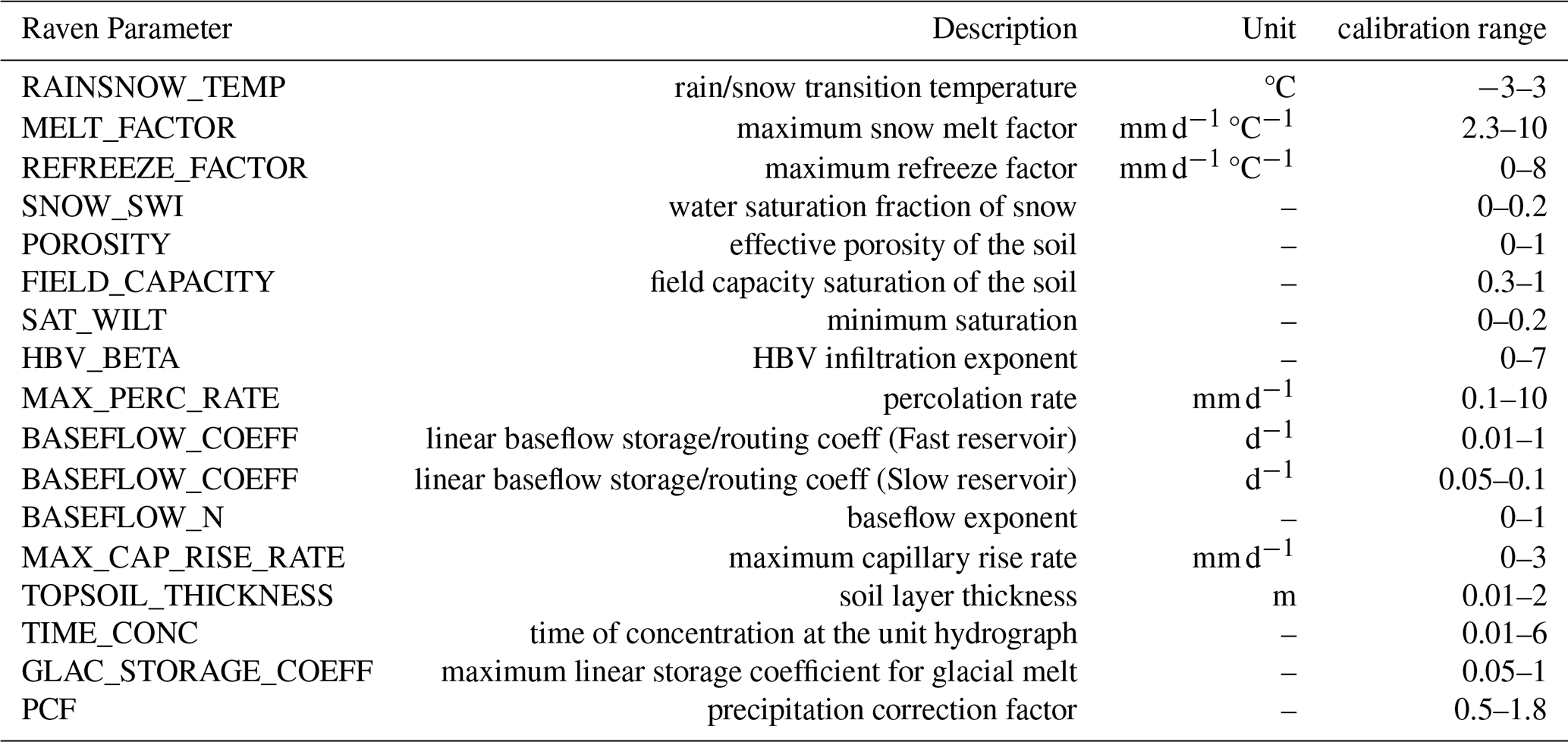
For this study, we emulate the HBV (Hydrologiska Byråns Vattenbalansavdelning) model, a conceptual precipitation-streamflow model (Bergström, 1995). HBV is widely applied in mountainous catchments and includes a simple glacier melt parameterization, making it well-suited for comparing simulated glacier melt between its native glacier module and GloGEM. The HBV glacier model calculates the melt rate based on the potential melt and a glacial melt correction factor applied to the degree-day factor of snow (f_{MELT_FACTOR}) (Table 2). No glacier melt occurs if there is any snow cover on the glacier area. The calculated meltwater is then released with a simple linear storage coefficient approach, where the glacier storage coefficient is a calibrated model parameter (f_{GLAC_STORAGE_COEFF}). The snow routine determines whether precipitation falls as rain or snow according to a temperature threshold (f_{RAINSNOW_TEMP}). Snowmelt is modeled using a modified degree-day method where the melt factor (f_{MELT_FACTOR}) varies seasonally between minimum and maximum values and is adjusted for forest cover and terrain aspect. The model accounts for the refreezing of liquid water during periods below freezing temperature (f_{REFREEZE_FACTOR}). Snow-covered area can be diagnosed at each time step as the areal sum of snow-covered HRUs, where an HRU counts as fully snow-covered whenever it holds non-negligible snow water equivalent. Precipitation input can additionally be scaled by a precipitation correction factor (f_PCF) to account for forcing uncertainty in high elevation catchments, as described in Sect. 3.4. HBV has two conceptual groundwater reservoirs: an upper zone for quick response (interflow) and a lower zone for baseflow. Each is depleted by linear recession equations with different coefficients (f_{BASEFLOW_COEFF}). The transfer function translates HRU outflow into river discharge using a triangular weighting function (f_{TIME_CONC}). For a more detailed description of model components the reader is referred to the Raven User's and Developer's Manual (Craig and the Raven Development Team, 2025). Parameter ranges for the HBV emulation were taken from the RavenPy repository (https://github.com/CSHS-CWRA/RavenPy.git, last access: 5 October 2026).

Table 2 Description of Raven parameters to emulate HBV and their calibration range.

3.3 Coupling approach

Following preprocessing of meteorological forcing and geospatial data for the selected catchment (Fig. 2A), GloGEM is calibrated and run by providing a list of RGI v6.0 IDs for glaciers within the catchment boundary. GloGEM provides daily glacier runoff, which includes ice melt, snowmelt, and rainfall from the initially glacierized area based on RGI v6.0 (RGI Consortium, 2017) (Fig. 2B; Huss and Hock, 2018), but does not account for baseflow or runoff–streamflow transformation.

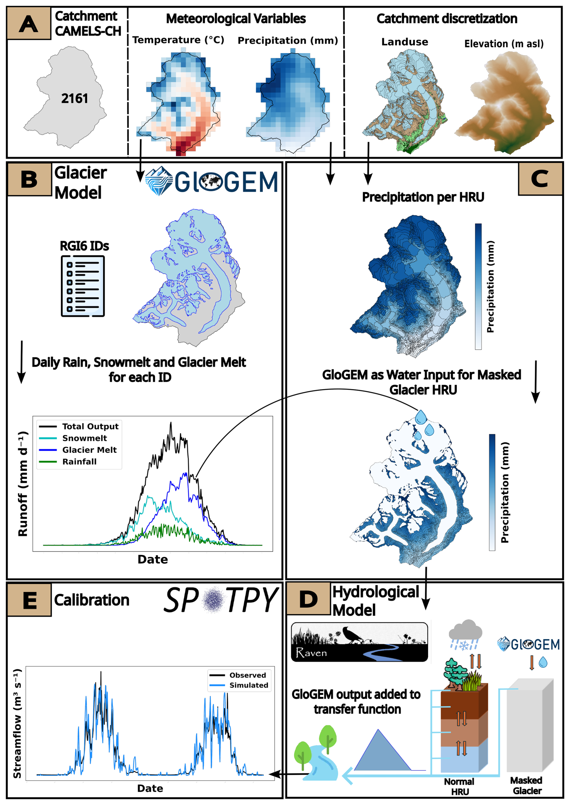
Figure 2 Workflow of the coupled GloGEM-Raven configuration. (A) Selection of the catchment ID and preprocessing of input data files. (B) Calibrating and running the glacier model GloGEM for each glacier in the catchment. (C) Calculating precipitation for each HRU and using GloGEM output as water input for glaciated areas. (D) Internal mechanism of Masked Glacier HRUs adding GloGEM output directly to the triangular transfer function. (E) Calibration of the model with Spotpy.

For the hydrological model, the catchment is discretized into HRUs based on the DEM, using 100 m elevation bands, landuse class and glacier outlines. It should be noted that HRUs regroup grid cells with similar landuse and elevation, but these grid cells can be spatially disconnected. The number of elevation bands and HRUs for each catchment is provided in the supplementary material (Table S1 in the Supplement). Precipitation and temperature inputs for each HRU are derived using spatially weighted averaging of gridded meteorological data from MeteoSwiss products (Fig. 2C). To integrate GloGEM outputs into Raven, we implemented a one-way coupling in which glacier runoff simulated by GloGEM replaces the precipitation input over glacier-covered areas in Raven.

The Raven model was modified to ensure that glacier runoff is directly added to the runoff-streamflow transfer function, in order to bypass intermediate storage components and preserve the timing and magnitude of glacier contributions. To achieve this, a new landuse called Masked Glacier is implemented in the model (Fig. 2D). In this model configuration, Masked Glacier landuse is defined with zero soil layers to prevent water infiltration into any subsurface storage, and evaporation is set to 0 to avoid any loss to the atmosphere, as this is already accounted for in GloGEM. The air temperature for Masked Glacier HRUs is set to 20 °C, thus avoiding any snow accumulation. Lastly, any precipitation corrections are disabled for Masked Glacier HRUs. These modifications ensure that glacier contributions are accurately reflected in the simulated streamflow (Fig. 2D).

This also changes how glacier meltwater is routed relative to the uncoupled configurations. In the native HBV glacier module, ice melt is released through a linear reservoir governed by a calibrated coefficient (f_{GLAC_STORAGE_COEFF}) before entering the catchment transfer function. This reservoir acts on glacier ice melt alone, and does not apply to snowmelt or rainfall. In the coupled configurations, our coupling uses GloGEM's aggregated runoff flux, in which ice melt, snowmelt, and rainfall are already combined and cannot be routed selectively. Since a large part of this combined flux consists of snowmelt and rainfall, passing all of it through the glacier reservoir would delay water that never enters that reservoir in the uncoupled setup. Consequently, we incorporate the aggregated GloGEM runoff directly into the catchment transfer function, thereby bypassing the linear glacier reservoir. As a result, the coupled model configurations require the calibration of one parameter fewer (Table 3).

Table 3 Model configurations and number of calibrated parameters used in this study.

3.4 Precipitation correction

Precipitation in high-elevation catchments is subject to substantial uncertainty. Observed precipitation can be underestimated due to gauge undercatch, which is particularly pronounced for solid precipitation and can reach up to 50 % (Goodison et al., 1998; Rasmussen et al., 2012). In addition, the spatial distribution of precipitation at high elevations is poorly constrained, as gauge networks are typically biased towards lower elevation (Frei and Schär, 1998). To account for these biases, the hydrological model includes a precipitation correction factor (f_PCF), a spatially and temporally uniform multiplier applied to all observed precipitation values at every time step. The PCF is not intended to represent a single process, but lumps these sources of uncertainty into one correction, as is common in comparable model applications (van Tiel et al., 2020). It is calibrated against streamflow within the range 0.5–1.8 (Table 2), together with the other hydrological model parameters.

A conceptually similar correction is already applied within GloGEM through its precipitation factor f_{c, prec}, but the two factors are distinct and independent. GloGEM's f_{c, prec} is calibrated against geodetic mass balance, prior to and independently of the hydrological calibration, and is therefore fixed before the hydrological model is calibrated. It is glacier-specific, with a separate value for each glacier, and additionally absorbs processes such as snow accumulation on the glacier from the surrounding slopes. It is thus only meaningful over the glacierized area and cannot be transferred to the non-glacierized part of the catchment. The PCF, in contrast, is calibrated against streamflow. In the uncoupled HBV configurations, it corrects precipitation over the entire catchment, whereas in the coupled HBV-GloGEM configurations, the Masked Glacier HRUs have precipitation correction disabled (Sect. 3.3), so the PCF acts only on the non-glacierized area. The two corrections therefore operate on spatially distinct parts of the catchment and are not interchangeable. As a consequence, a precipitation correction is embedded in every coupled configuration through the GloGEM runoff, which already carries f_{c, prec}, while the hydrological PCF is applied only in the dedicated PCF configurations. Therefore the total water volume entering the catchment differs between configurations.

Implementing PCF only in dedicated model configurations (Table 3) allows us to isolate its effect through comparisons between simulations with and without the PCF. Each configuration in this study corresponds to a separate calibration run with its own parameter set. Conceptual glacier routines are known to compensate for biases in the precipitation forcing by adjusting simulated glacier melt (Stahl et al., 2008; Duethmann et al., 2015). Introducing the PCF in dedicated configurations therefore lets us test how an explicit precipitation correction affects the simulated melt partitioning and streamflow, and to compare this response between the coupled and uncoupled setups.

3.5 Snow redistribution

To avoid the unrealistic accumulation of snow at high elevations, we implemented a snow redistribution module in the Raven framework, based on the SnowSlide concept (Bernhardt and Schulz, 2010) and adapted for semi-distributed models. Snow transport is simulated when a slope-dependent snow-holding depth is exceeded, using the same parameterization as the FSM2trans snow-hydrological model (Quéno et al., 2024) and without any additional calibrated parameters. Snow exceeding the holding depth is transported laterally to connected HRUs at lower elevations (Fig. 3b). In contrast to the original grid-based formulation, where transport weights depend on elevation differences between cells, the semi-distributed approach weights lateral snow redistribution by the upstream area draining from one HRU into the next. To enable this lateral transport, HRU connectivity is derived during catchment preprocessing following the methodology of the HydroBricks modeling framework (Horton and Argentin, 2024). Specifically, surface depressions in the DEM are identified and filled following the method of Wang and Liu (2006). Flow direction and flow accumulation are then computed using the D8 flow routing algorithm (O'Callaghan and Mark, 1984) as implemented in the Python package pysheds (Bartos, 2020). Flow paths are traced between HRUs, with connection weights based on accumulated upstream area (Fig. 3a). Disconnected HRUs are linked to the nearest neighbour by centroid distance, ensuring complete catchment connectivity. The resulting connectivity information is then provided to Raven as an external input. Depending on the selected configuration, an HRU can be connected either to a single downstream HRU or to multiple HRUs at lower elevations.

Snow redistribution also induces temporal shifts in the relative contributions of snowmelt and glacier melt (Fig. 3b). In the native HBV glacier module, no ice melt occurs while the glacier is snow-covered. Because glacier surfaces are generally flatter than the surrounding terrain, glacierized HRUs tend to receive redistributed snow. This prolongs their snow cover and delays ice melt. The redistributed snow instead melts at lower, warmer elevations, so melt shifts from glacier ice toward snow. This mechanism applies only to the uncoupled configurations. In the coupled configurations the glacier is represented by the Masked Glacier HRUs (Sect. 3.3), whose runoff is supplied entirely by GloGEM; because GloGEM already accounts for snow accumulation, redistribution, and melt on the glacier, any snow redistributed onto these HRUs would be double-counted and is therefore removed.

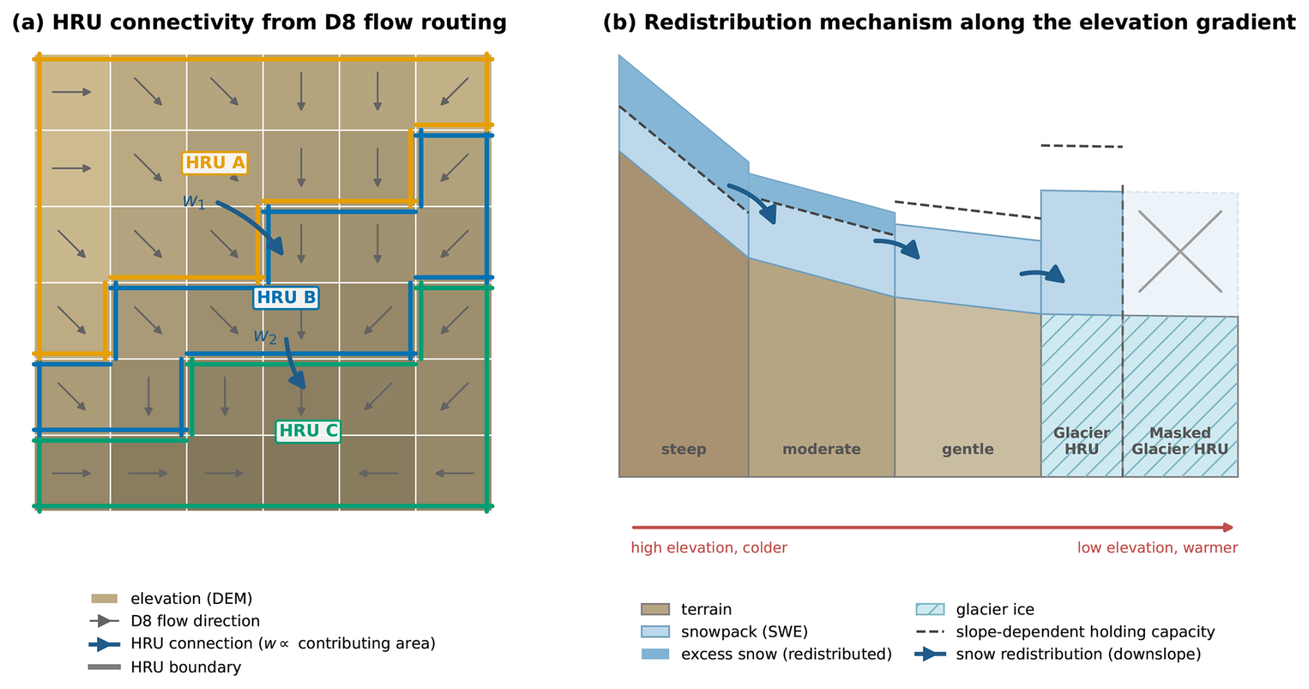
Figure 3 Schematic of the snow redistribution scheme. (a) HRU connectivity derived from D8 flow routing: connections between HRUs follow the flow direction, with weights (w) proportional to the upstream area draining from one HRU into the next. (b) Redistribution along the elevation gradient: snow exceeding the slope-dependent holding capacity (dashed line) is transferred downslope (blue arrows) to lower HRUs. Snow redistributed onto Masked Glacier HRUs is removed, as GloGEM accounts for the glacier.

3.6 Calibration

GloGEM is calibrated to match simulated glacier-specific mass balance with observed geodetic mass balance from Hugonnet et al. (2021), aiming to reproduce the long-term trend of glacier evolution for each individual glacier over the period 2000–2019 (Zekollari et al., 2024). Throughout calibration, the glacier area is kept constant. Three parameters are optimized sequentially: f_{c, prec}, a multiplicative precipitation correction factor; f_{dd, snow}, the degree-day factor for snow (with f_{dd, ice}=2f_{dd, snow}), which links air temperature to melt rates; and f_{t, offset}, a local temperature correction term. Initial estimates are f_{c, prec}=0.8 (range: 0.8–5.0), f_{dd, snow}=3 mm d⁻¹ °C⁻¹ (range: 1.75–4.5), and f_{t, offset}=0 °C (Hock, 2003). The calibration is carried out in three sequential phases: first, f_c,prec is adjusted to account for precipitation uncertainty and local orographic effects; if the target tolerance is not achieved, f_{dd, snow} is optimized while keeping f_{c, prec} constant; finally, if necessary, f_{t, offset} is adjusted to correct systematic temperature biases. Convergence is considered achieved when the difference between simulated and observed mass balance falls within a predefined tolerance, set arbitrarily between 0.01 and 0.05 m w.e. yr⁻¹ (Zekollari et al., 2024).

The Raven calibration routine is established using the Python Spotpy package (Houska et al., 2015) (Fig. 2E). The Shuffled Complex Evolution (SCE-UA) algorithm is used for the calibration process (Duan et al., 1993). The number of iterations to achieve convergence is set to 10 000 and the number of complexes is 15. In this study, all selected catchments are calibrated for the period 1 January 2000 to 31 December 2009 and evaluated from 1 January 2010 to 31 December 2020. Calibration is performed against observed daily streamflow, using the Kling–Gupta Efficiency (KGE; Gupta et al., 2009) as the objective function, which contains correlation, bias, and variability components. For model evaluation, the Nash–Sutcliffe Efficiency (NSE; Nash and Sutcliffe, 1970) is additionally reported. No snow or SWE data are used in the calibration. The gridded SPASS product is reserved for the independent validation of simulated SWE. All configurations and catchments are initialized following the same scheme. Snow water equivalent and the upper soil store are set to zero on the first time step and the lower groundwater reservoir is initialized to half of the topsoil water-holding capacity to avoid starting the slow reservoir empty. Model performance is reported for the validation period (2010–2020), for which the initial values are taken from the preceding calibration period. All reported performance metrics are computed on full time periods, without a warm-up period to account for model reservoir initialization. This leads to some initialization effects (in particular for snow) in the first year of the calibration period. These cannot be removed consistently by a common warm-up window, as the configurations without snow redistribution never reach a stationary high-elevation snow state, while the validation period itself starts from model states carried over from ten years of continuous simulation.

Six model configurations are calibrated for each catchment (Table 3). The first three configurations use the native HBV glacier module: (1) baseline HBV with 15 calibrated parameters, (2) HBV with snow redistribution (HBV-SR, 15 parameters), and (3) HBV with snow redistribution and a calibrated precipitation correction factor (HBV-PCF, 16 parameters). The remaining three configurations employ the coupled models: (4) HBV-GloGEM, (5) HBV-GloGEM-SR with snow redistribution, and (6) HBV-GloGEM-PCF with snow redistribution and precipitation correction. The coupled configurations require one parameter fewer since the linear glacier outflow parameter of HBV's glacier model is not used.

4 Results

4.1 Streamflow performance

Figure 4a presents KGE and NSE values for all catchments over the validation period. The KGE results indicate that uncoupled HBV configurations slightly outperform coupled configurations, with median KGE values for HBV configurations ranging between 0.84 and 0.87 compared to median KGE values ranging from 0.81 to 0.87 for HBV-GloGEM configurations, with the difference nearly vanishing for the configurations that include a precipitation correction factor. In terms of NSE, the two configuration groups show relatively similar performance, with median values of 0.78–0.79 for HBV and 0.77–0.78 for HBV-GloGEM. Model performance is generally similar with the addition of snow redistribution. The application of a precipitation correction factor improves KGE and NSE for most catchments. A table with all KGE and NSE values is provided in the supplementary material (Tables S2 and S3).

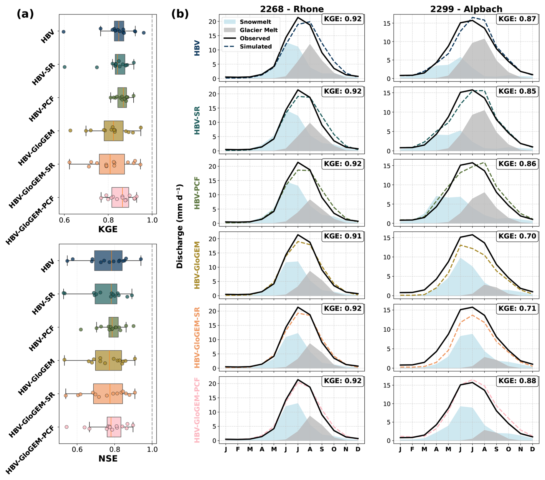
Figure 4 (a) KGE and NSE values for the validation period for all configurations and all catchments are shown in a boxplot. (b) Streamflow regime (monthly averaged values), glacier melt regime and snowmelt regime during the entire validation period for all configurations and two representative catchments, Rhone (ID 2268) and Alpbach (ID 2299).

Figure 4b illustrates streamflow regimes, glacier melt, and snowmelt for the validation period in two representative catchments. The left column shows simulations compared to observed streamflow for the Rhone catchment, which has a glacierized area of 44.1 % in the year 2000. The standard HBV configuration overestimates late-season streamflow and underestimates early melt season discharge, which was found across many study catchments. Snow redistribution partially addresses this issue. The coupled HBV-GloGEM model better captures late-summer streamflow, but fails to reproduce peak summer discharge without precipitation correction. The Alpbach catchment (right column), which has a glacierized area of 22.1 % in the year 2000, exhibits similar temporal biases, with underestimated early-season and overestimated late-season streamflow. The HBV-GloGEM and HBV-GloGEM-SR configurations struggle to reproduce observed streamflow due to insufficient water availability. However, incorporating a precipitation correction factor substantially improves model performance. The different model configurations produce substantially different glacier melt and snowmelt dynamics, both in magnitude and seasonal timing, with the strongest contrasts observed in the less glacierized Alpbach catchment.

4.2 Glacier melt

To evaluate the simulated glacier melt, we use the glacier melt dataset for Switzerland described in the work of van Tiel et al. (2026), hereafter referred to as the reference melt. The results show that GloGEM reproduces the reference melt more accurately than the hydrological model (Fig. 5). The HBV glacier module consistently overestimates melt, except in catchments with very low glacier cover such as the Goneri and Reuss. Incorporating snow redistribution in the model often reduces simulated HBV melt, bringing results closer to the reference melt in catchments where overestimation occurs. This effect is particularly noticeable in the highly glaciated Massa catchment, where the HBV-SR configuration agrees well with the reference melt. Introducing a precipitation correction factor further reduces simulated melt in most catchments; for example, in the Simme catchment, the HBV glacier module reproduces the reference melt well when the correction factor is applied (HBV-PCF). However, overestimation remains in most catchments. As GloGEM uses geodetic mass balance for calibration, it is expected to better reproduce the glacier mass balance across Switzerland.

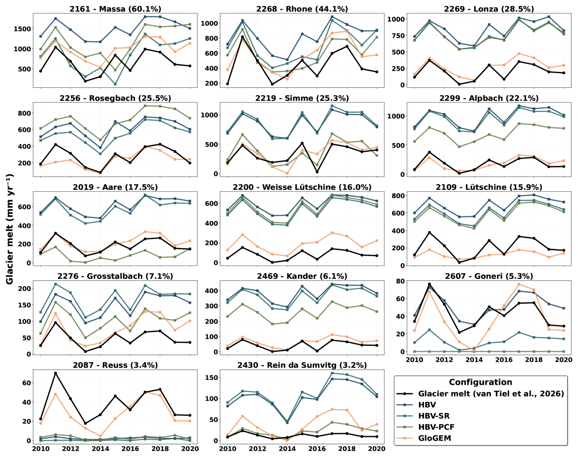
Figure 5 Glacier melt (van Tiel et al., 2026) and simulated glacier melt for 14 Swiss catchments, the different HBV configurations, and GloGEM.

4.3 SWE performance

Simulated catchment-average snow water equivalent (SWE) was validated against the 1 km gridded SPASS dataset (Marty et al., 2025a) (Fig. 6). The root mean square error (RMSE) is computed based on the daily catchment average SWE (only non-glacier area) of the SPASS dataset and simulated SWE. In the HBV and HBV-GloGEM configurations, the simulations show a continuous increase in catchment-average SWE, indicating unrealistic snow accumulation in higher-elevation HRUs (Freudiger et al., 2017). The median RMSE is 243 and 184 mm, respectively, suggesting that catchment-average SWE is poorly represented when snow redistribution is not included in the model. Incorporating snow redistribution substantially improves the representation of catchment-average SWE, as seen for HBV-SR with a median RMSE of 142 mm and for HBV-GloGEM-SR with a median RMSE of 134 mm, showing strong agreement with the SPASS dataset. When applying a precipitation correction factor, SWE remains well represented for the HBV-PCF configuration (145 mm) but deteriorates for the HBV-GloGEM-PCF configuration (166 mm). The latter generally requires a higher precipitation correction factor (Fig. S23), which can result in excessive snow input and consequently reduces model performance for SWE.

Beyond the catchment average, simulated SWE was also evaluated per elevation band (Fig. S19). The configurations with snow redistribution reproduce the seasonal SWE of the SPASS reference across low and mid elevation bands, confirming that the vertical distribution of snow, not only the catchment mean, is captured. The unrealistic accumulation in the HBV and HBV-GloGEM configurations is concentrated in the highest bands, where SWE grows without bound, whereas the redistribution configurations prevent it.

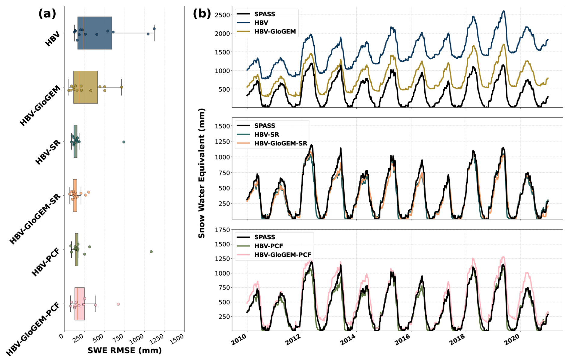
Figure 6 (a) Catchment average (non-glacier area) SWE performance calculated with RMSE for all catchments and configurations. (b) Time series of catchment average (non-glacier area) SWE in the validation period for the Rhone catchment (ID 2268) and all six model configurations. The differing SWE between configurations at the start of the period reflects the divergent snow storage each configuration accumulated over the calibration period under its own parameter set.

4.4 Model parameters

Calibrating the model under different configurations leads to shifts in parameter distributions, particularly for snow and melt parameters. Figure 7a presents the melt factor in mm d⁻¹ °C⁻¹ for the 100 best parameter sets across the nine most glaciated catchments with more than 10 % glacier cover, for which the model coupling has the strongest influence on parameter behavior. Coupling HBV with GloGEM produces the largest shifts in melt factor values compared to the original HBV configurations, consistently resulting in lower calibrated melt factors. Including snow redistribution has little influence on the melt factor, while the precipitation correction factor affects melt parameters only in a small number of catchments. The precipitation correction factor shows the second clear and consistent response (Fig. 7b). In each of the nine catchments, the calibrated precipitation correction factor is higher in the coupled HBV-GloGEM-PCF configuration than in the uncoupled HBV-PCF configuration. Notably, the two parameters with the most consistent cross-catchment response shift in opposite directions under coupling: the melt factor decreases, while the precipitation correction factor increases. The remaining snow parameters – the rain/snow transition temperature, the refreeze factor, and the snow water-holding capacity – do not show a consistent directional response to the configuration changes. Their shifts are catchment-specific and lack a clear cross-catchment pattern. Their distributions are provided in the Supplement (Figs. S20–S22).

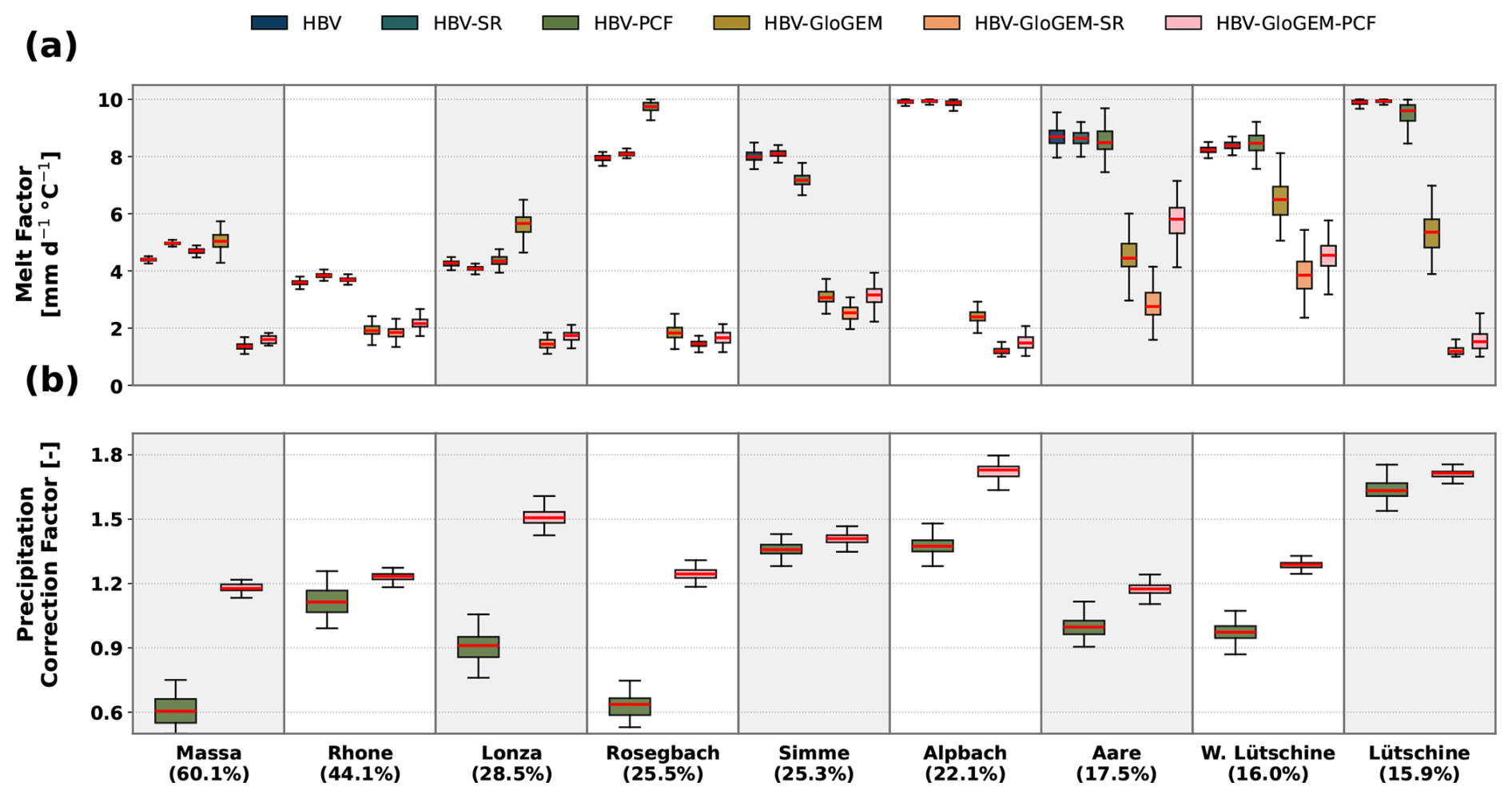
Figure 7 Calibrated parameter values for the 100 best parameter sets in the nine catchments with more than 10 % glacier cover, ordered by decreasing glacierized area; the percentage below each catchment name gives the glacierized area in the year 2000. (a) Melt factor (f_{MELT_FACTOR}) for all six model configurations. (b) Precipitation correction factor (f_PCF) for the two configurations that include it (HBV-PCF and HBV-GloGEM-PCF).

4.5 Uncertainty

Applying a precipitation correction factor improves streamflow performance but also increases the uncertainty in estimating glacier and snowmelt contributions. Figure 8a illustrates the streamflow, glacier melt, and snowmelt regimes for the 20 best parameter sets for the Rhone catchment. The Rhone catchment exemplifies equifinality, where multiple parameter sets yield similarly good streamflow performance but substantially different melt dynamics. For the HBV-PCF configuration, simulated annual glacier melt contributions range from 11 % to 38 %, while snowmelt contributions vary between 51 % and 73 %. Figure 8b shows the coefficient of variation (CV) in melt estimates for the nine catchments with the highest glacier coverage. Catchments with very little glacier melt are not shown, as CV values in those catchments become extremely high and do not reflect meaningful variability. The CV of glacier melt is markedly higher for the HBV-PCF configuration than for the other HBV setups, reflecting increased sensitivity when a precipitation correction factor is applied. As expected, GloGEM configurations show no variation in glacier melt because it is provided as a fixed input. Snowmelt uncertainty also rises under the HBV-PCF configuration, reaching its highest values in the most glaciated catchments.

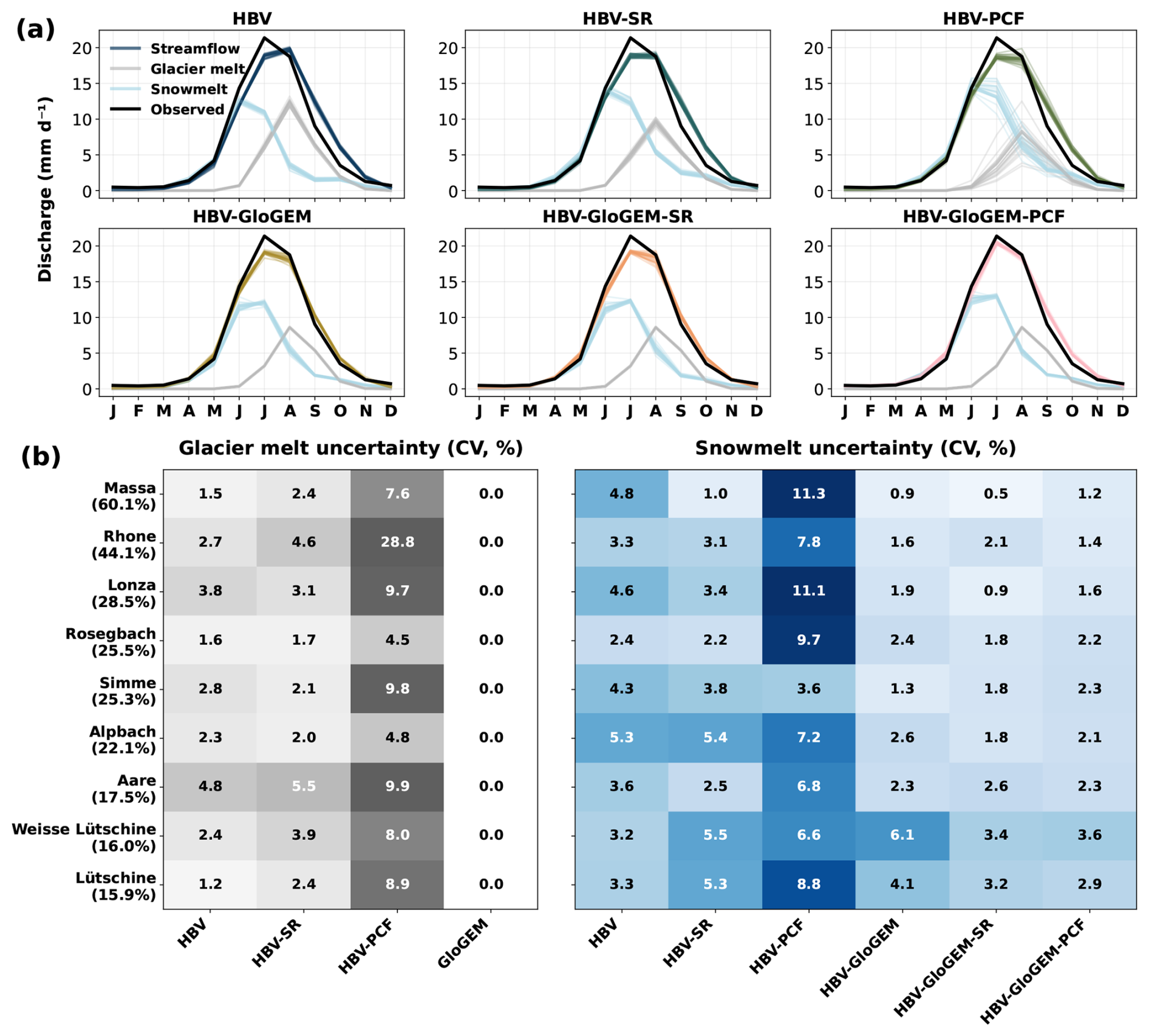
Figure 8 (a) Streamflow regimes, glacier melt regimes and snowmelt regimes for the validation period for all configurations for the 20 best parameter sets in the Rhone (ID 2268) catchment. (b) The coefficient of variation (CV) calculated for the nine most glaciated catchments and all configurations for annual snowmelt and glacier melt.

4.6 Annual contributions

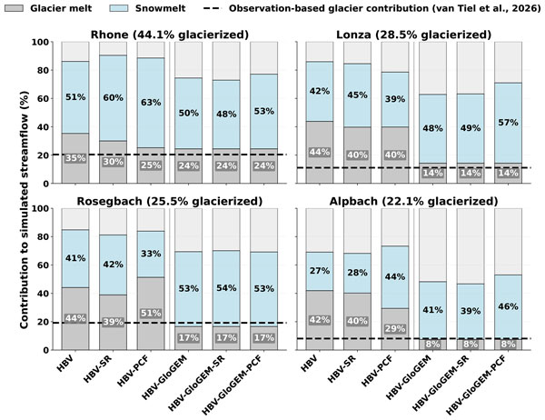
Annual melt contributions vary substantially across model configurations within each catchment (Fig. 9). For HBV configurations, snow redistribution has a pronounced effect: snowmelt contributions increase and glacier melt decreases in most catchments, while total melt remains relatively constant. This is expected, as snow redistribution allows snow that was previously inaccessible in “snow towers” to become available for melt. The impact of precipitation correction on annual melt partitioning is configuration-dependent and lacks a consistent directional pattern. For instance, in the Massa catchment, precipitation correction increases glacier melt contributions, whereas in the Simme catchment it substantially reduces glacier melt, bringing simulations into close agreement with the reference melt contributions (van Tiel et al., 2026). In contrast, snow redistribution has minimal impact on melt partitioning in HBV-GloGEM configurations. However, precipitation correction consistently increases snowmelt contributions across most catchments in the coupled model. Comparing glacier representations, HBV-GloGEM configurations generally reproduce the reference glacier melt contributions well, whereas HBV configurations systematically overestimate glacier melt across catchments.

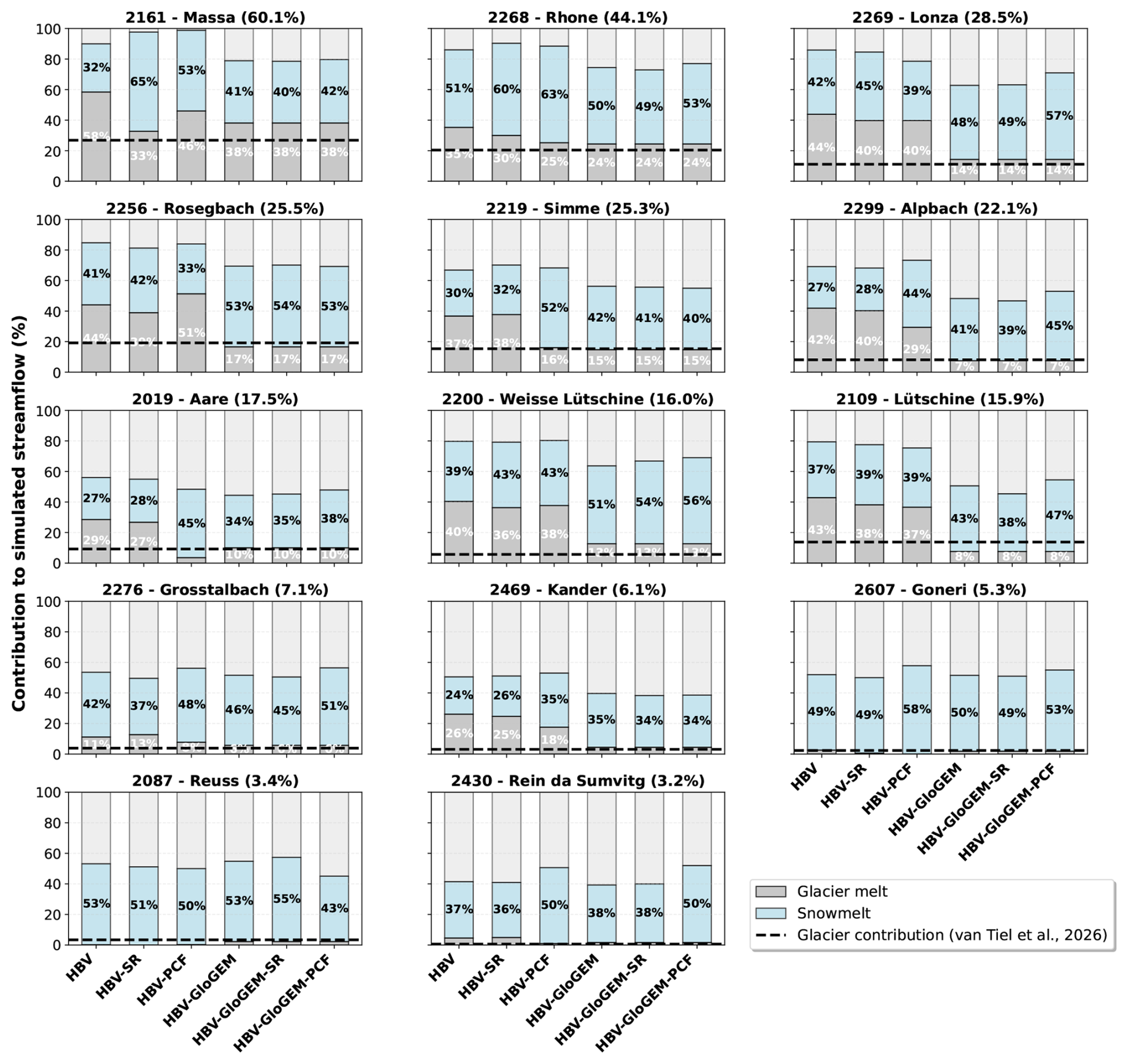
Figure 9 Annual contributions from glacier and snowmelt in % to the annual streamflow for all catchments and each configuration.

5 Discussion

In this study, we coupled the hydrological modeling framework Raven (Craig et al., 2020), emulating HBV, with the Global Glacier Evolution Model GloGEM (Huss and Hock, 2015) and implemented a snow redistribution scheme to improve process representation in 14 glaciated catchments across the Swiss Alps. We investigated whether introducing additional constraints through glacier model coupling and improved snow distribution could reduce parameter equifinality and improve the quantification of seasonal snow and glacier melt contributions.

The uncoupled HBV configurations consistently outperformed the coupled HBV-GloGEM setups according to calculated streamflow metrics (KGE and NSE). This contrasts with findings from recent coupling studies that reported improved streamflow simulations when integrating global glacier models (Wiersma et al., 2022; Hanus et al., 2024). However, these studies coupled global glacier models with global hydrological models that previously lacked any glacier representation. Only Pesci et al. (2023) compared a coupled model against a traditional volume-area scaling approach, finding similar streamflow performance in a single Austrian catchment. Our results across 14 Swiss catchments reveal more complex patterns, with some catchments showing comparable performance between configurations while others exhibiting substantial discrepancies.

While original HBV configurations achieve better streamflow metrics, they do so by simulating glacier melt rates that exceed both GloGEM estimates and the reference glacier mass loss (van Tiel et al., 2026) by factors of two to three in some catchments. The HBV glacier module provides additional degrees of freedom during calibration, allowing the glacier component to compensate for various model deficiencies, including process representation limitations and input data biases (Duethmann et al., 2015; He et al., 2015). This compensation primarily results from precipitation underestimation in the forcing data, a challenge in complex mountain terrain where spatial interpolation errors can be substantial (Immerzeel et al., 2014; Henn et al., 2018). To a lesser extent, uncertainties in solid-liquid precipitation partitioning may also influence model behavior (Magnusson et al., 2011). The HBV glacier model responds to these deficiencies by amplifying melt rates during calibration, effectively using glacier ice as an adjustment variable to close the water balance.

This compensation mechanism is particularly problematic when attempting to quantify individual melt contributions. A key challenge is parameter equifinality (Beven, 2006), where multiple parameter combinations can produce equally good streamflow simulations while implying vastly different snow and glacier melt estimates. Without precipitation correction, HBV systematically overestimates glacier melt. With precipitation correction included, the model gains an additional degree of freedom, creating trade-offs between the precipitation correction factor and glacier melt parameters. Stahl et al. (2008) showed that equivalent streamflow simulations can correspond to widely varying glacier mass balance estimates. Our uncertainty analysis confirms this pattern, where among the 20 best-performing parameter sets, simulated glacier melt contributions vary substantially. This has important implications for climate impact studies. Models that perform well due to compensating errors may misrepresent key components of the present-day water balance. As a result, they are unlikely to provide reliable projections under future conditions as melt contributions to streamflow shift under a changing climate.

Constraining the glacier component with an independent observation of glacier mass change offers a way to reduce the reliance on streamflow data alone. Coupling with GloGEM achieves this by calibrating glacier evolution against observed geodetic mass balance (Hugonnet et al., 2021), yielding glacier melt estimates that align with the reference glacier mass loss across Switzerland. This raises the question of whether the improved realism stems from the coupling itself or from the different data used to constrain the glacier component, since in our uncoupled setup the native HBV glacier routine is constrained only by streamflow. Previous studies have incorporated glacier-wide or point mass-balance data into the calibration of conceptual and distributed glacio-hydrological models (Konz and Seibert, 2010), and such multi-objective calibration can reduce equifinality in the simulated melt components (Finger et al., 2015; van Tiel et al., 2020). When applied to a semi-distributed model such as ours, however, this constraint remains weak, as the model applies a single set of degree-day parameters across all glacier HRUs, so the per-glacier geodetic estimates (Hugonnet et al., 2021) would have to be collapsed into one catchment-average target, averaging over glaciers of differing characteristics. The model further treats glacier ice as an unlimited reservoir with no accumulation mechanism, so it cannot close the glacier mass budget that a meaningful comparison against geodetic observations would require. GloGEM, in contrast, calibrates parameters individually for each glacier from its area–altitude distribution, and can therefore exploit the full spatial resolution of global geodetic mass-balance products. In our framework, coupling and constraint are therefore not independent choices, since it is precisely the dedicated glacier model that makes the per-glacier geodetic constraint informative.

Beyond constraining glacier evolution, accurately representing snowmelt contributions requires realistic simulation of snow accumulation patterns in complex mountain terrain. Snow redistribution processes remain poorly represented in glacio-hydrological modeling, with van Tiel et al. (2020) finding that only 20 % of published studies explicitly account for these processes. Neglecting snow redistribution results in unrealistic snow accumulation at high elevations, as observed in most catchments in this study. Our implementation uses a simplified gravitational redistribution scheme (Freudiger et al., 2017), a common approach in hydrological modeling that does not simulate the actual physical processes of wind drift and avalanches. Despite this simplification, the snow redistribution scheme successfully prevents unrealistic snow tower formation (Frey and Holzmann, 2015) and improves melt partitioning. Redistributing snow to lower, warmer elevations increases the proportion of melt originating from snow rather than glacier ice, producing more physically consistent melt contributions that align better with observations.

6 Limitations and future work

A first limitation concerns how the glacier component is constrained. GloGEM's calibration against geodetic mass balance (Hugonnet et al., 2021) is itself subject to equifinality, as multiple parameter combinations can reproduce the observed mass balance (Gabbi et al., 2014; von der Esch et al., 2025), although this remains the standard approach for global glacier models (Rounce et al., 2023; Zekollari et al., 2024). Moreover, the improved realism of the coupled setup cannot be attributed to the coupling alone, because the coupled and uncoupled configurations differ both in whether the glacier is coupled and in the data used to constrain it. Exploiting a per-glacier geodetic constraint requires a model that resolves individual glaciers, which the native HBV routine does not and which glacier models such as GloGEM already provide efficiently. The two effects therefore cannot be cleanly separated within our framework and remain intertwined in the comparison.

A second limitation relates to the routing of glacier meltwater in the coupled configurations. Bypassing the linear glacier reservoir removes the storage delay that buffers ice-melt release in the uncoupled configurations. Although GloGEM computes ice melt, snowmelt, and rain on the initial glacier area separately, our coupling supplies the total glacier runoff to Raven as a single glacier runoff input, so this delay cannot be applied to the ice-melt fraction alone. Future coupling schemes could pass these components separately, allowing the ice-melt fraction to be routed through a glacier release storage.

A third limitation concerns the evaluation of the simulated snow, which we assess against the gridded SPASS product rather than against snow-covered area (SCA). Although SCA is directly observed and widely used to constrain hydrological models, it is a proxy for snow presence. Because of the hysteresis between SWE and SCA (Riboust et al., 2019), a given snow-covered area does not determine the snow amount that drives streamflow. Diagnosing SCA in Raven would moreover require a snow depletion curve, that is, an assumed relationship between the simulated SWE and the fraction of the area that is snow-covered. A comparison against observed SCA would then evaluate this assumed relationship together with the simulated snowpack. We therefore evaluate against SWE, using the gridded, observation-assimilated SPASS product, while noting that SPASS is itself model-based and that observed SCA remains a valuable complementary constraint, particularly where no gridded SWE product is available.

Future work could further reduce parameter equifinality by incorporating additional observational constraints beyond geodetic mass balance and streamflow. Glacier model calibration could be refined using seasonal snowline observations, which provide stronger constraints on glacier ablation patterns than annual mass balance alone (Barandun et al., 2018; Cremona et al., 2025). Similarly, remote sensing snow cover products offer potential for constraining the hydrological model's snow accumulation and melt processes (Parajka and Blöschl, 2008; Di Marco et al., 2021). However, given that constraining glacier evolution already substantially improves snowmelt identifiability through reduced compensatory adjustments, the marginal benefit of additional snow cover constraints requires further investigation.

7 Conclusions

Mountain regions face substantial hydrological changes as climate warming alters snow and glacier melt dynamics. Accurately projecting these changes requires hydrological models that correctly partition melt contributions between snow and glacier sources. This study investigated whether coupling the hydrological model Raven with the Global Glacier Evolution Model GloGEM and implementing snow redistribution could reduce parameter equifinality and improve melt contribution estimates. We applied this framework to 14 headwater catchments in Switzerland, comparing six model configurations that varied in glacier representation, snow redistribution, and precipitation correction. Our analysis reveals a fundamental challenge: models achieving superior calibration performance do not necessarily provide accurate process representation. While uncoupled HBV configurations outperformed coupled HBV-GloGEM setups by streamflow metrics, they did so by simulating glacier melt 2–3 times higher than reference datasets to compensate for precipitation biases in the forcing data. Applying a precipitation correction factor produced severe parameter equifinality, with glacier melt varying substantially between equally well performing parameter sets. Coupling with GloGEM, constrained by geodetic mass balance, improved the identifiability of both melt components while simulating glacier melt consistent with the reference dataset. Snow redistribution further enhances model reliability by addressing unrealistic accumulation patterns. For mountain hydrology under climate change, these results carry important implications. Models calibrated solely on streamflow can achieve good historical performance while misrepresenting the processes that determine future behavior. This is a critical limitation as warming alters melt dynamics. Our work demonstrates that coupling a hydrological model with a global glacier model provides a more reliable framework for climate impact assessments, even though this results in a minor reduction in historical performance metrics. Future advances could integrate additional constraints, such as seasonal snowline observations or snow cover products, to further increase the identifiability of melt contributions.