the Creative Commons Attribution 4.0 License.
the Creative Commons Attribution 4.0 License.
 | 04 Feb 2026
When physics gets in the way: an entropy-based evaluation of conceptual constraints in hybrid hydrological models
Manuel Álvarez Chaves
Eduardo Acuña Espinoza
Uwe Ehret
Anneli Guthke
Merging physics-based with data-driven approaches in hybrid hydrological modeling offers new opportunities to enhance predictive accuracy while addressing challenges of model interpretability and fidelity. Traditional hydrological models, developed using physical principles, are easily interpretable but often limited by their rigidity and assumptions. In contrast, machine learning methods, such as Long Short-Term Memory (LSTM) networks, offer exceptional predictive performance but are often criticized for their black-box nature. Hybrid models aim to reconcile these approaches by imposing physics to constrain and understand what the ML part of the model does. This study introduces a quantitative metric based on Information Theory to evaluate the relative contributions of physics-based and data-driven components in hybrid models. Through synthetic examples and a large-sample case study, we examine the role of physics-based conceptual constraints: can we actually call the hybrid model “physics-constrained”, or does the data-driven component overwrite these constraints for the sake of performance? We test this on the arguably most constrained form of hybrid models, i.e., we prescribe structures of typical conceptual hydrological models and allow an LSTM to modify only its parameters over time, as learned during training against observed discharge data. Our findings indicate that performance predominantly relies on the data-driven component, with the physics-constraint often adding minimal value or even making the prediction problem harder. This observation challenges the assumption that integrating physics should enhance model performance by informing the LSTM. Even more alarming, the data-driven component is able to avoid (parts of) the conceptual constraint by driving certain parameters to insensitive constants or value sequences that effectively cancel out certain storage behavior. Our proposed approach helps to analyse such conditions in-depth, which provides valuable insights into model functioning, case study specifics, and the power or problems of prior knowledge prescribed in the form of conceptual constraints. Notably, our results also show that hybrid modeling may offer hints towards parsimonious model representations that capture dominant physical processes, but avoid illegitimate constraints. Overall, our framework can (1) uncover the true role of constraints in presumably “physics-constrained” machine learning, and (2) guide the development of more accurate representations of hydrological systems through careful evaluation of the utility of expert knowledge to tackle the prediction problem at hand.
- Article
(7946 KB) - Full-text XML
- BibTeX
- EndNote


Hydrological models are essential tools for the management of water resources as well as scientific research. Due to their wide range of applications, the motivations and reasons behind the choices that lead to the specific usage of a model over another are not clear and the issue of adequacy in the choice of a model is not typically addressed (Horton et al., 2022). Worryingly, the choice of a model is often relegated to past experience and not adequacy (Addor and Melsen, 2019).
Some authors have argued for the creation of a Community Hydrology Model which could be able to represent different processes at different scales, making it suitable for a wide range of applications, but there are open challenges that need to be addressed before such a model can be developed (Weiler and Beven, 2015). In contrast, other authors support the concept of flexible modeling frameworks that enable users to combine different representations of processes and model constructs (Fenicia et al., 2011; Clark et al., 2008). Using this approach, a unique model can be developed for a specific application, and the issue of model adequacy is addressed by testing multiple models as different working hypotheses (Clark et al., 2011).
1.1 Conceptual rainfall-runoff models
So far, the traditional modeling approach has been that of simplified physical concepts in which different compartments in the hydrological cycle are represented by interconnected storage units and these models obey physical principles. Thus, understanding of the physical system is translated into the model and vice-versa, making the models easily interpretable.
Typically, catchment scale processes in a rainfall-runoff model are represented by a reservoir element that can be described by ordinary differential equations (ODEs):
where S(t) represents the conceptual storage of a reservoir element at time t, u(t) is time-dependent forcing data, Q(t) is the response of the reservoir element to the forcing and θ are the model parameters. Furthermore, f and g are functions that describe the evolution of storage and output with time (Fenicia et al., 2011). These types of models are physically-based because the main driving principle of a model is conservation of mass through Eq. (1).
These very simple principles for conceptual rainfall-runoff models have been adapted into modular modeling frameworks such as FUSE (Clark et al., 2008), Superflex (Fenicia et al., 2011; Dal Molin et al., 2021) and RAVEN (Craig et al., 2020). These frameworks enable researchers to develop an unlimited range of modular structures for rainfall-runoff models. In practice, researchers apply these frameworks in model comparison studies using one of typically two approaches: top-down or bottom-up development. The top-down approach begins with a complex model and reduces its components, while the bottom-up approach starts with a simple model and gradually increases its complexity (Hrachowitz and Clark, 2017).
Other studies evaluate an existing set of standard model structures within these frameworks. Although the choice of components is often arbitrary and informed by prior experience, a paradigm for automatic model structure identification has been proposed which systematically tests and identifies the most adequate model structures for a rainfall-runoff model while acknowledging the challenge of equifinality (Spieler et al., 2020).
1.2 LSTMs
Unlike the previous approach, machine learning (ML) and other purely data-driven approaches assume no prior knowledge and learn the required relationships between variables from the provided data alone. In particular, Long Short-Term Memory (LSTM) networks have been shown to provide very accurate predictions of streamflow establishing a number of benchmarks across different data sets (Kratzert et al., 2018, 2019b, c; Lees et al., 2021; Loritz et al., 2024). The performance of these models can be partly attributed to the flexibility of LSTM networks (LSTMs hereafter) which do not have the constraints that physically-based models have.
LSTMs (Hochreiter and Schmidhuber, 1997) are a type of recurrent neural network (RNN) which has been widely adapted in hydrology for rainfall-runoff modeling and/or predicting streamflow (Kratzert et al., 2024). More generally, RNNs and LSTMs have found applications in modeling dynamical systems (Gajamannage et al., 2023). Indeed, the reason they have been successful is that this type of neural network adds both memory (that is, states) and feedback to allow for the current output values to depend on past output values and states (Goodfellow et al., 2016). As mentioned previously, because a catchment can be represented as a set of ODEs which make it a dynamical system (Kirchner, 2009), the usage of LSTMs for rainfall-runoff modeling arises naturally. Ultimately, both approaches: conceptual and data-driven models are complementary, and direct mappings between one another have been identified (Wang and Gupta, 2024).
The issue of lacking mass conservation in LSTMs has been addressed by models which include an additional term that accounts for unobserved sinks, pointing towards deficiencies in data products (Frame et al., 2023) and this issue of closure is often a point of discussion and controversy (Beven, 2020; Nearing et al., 2021). Nevertheless, the main criticism of these models comes from their “black-box” nature, which makes their internal processes difficult to understand. Current methods for interpreting neural networks typically require the use of a secondary model to analyze the primary one (Montavon et al., 2018). For example, while researchers have proposed techniques to correlate LSTM hidden states with real-world variables (Lees et al., 2022), this interpretation process remains complex and requires the implementation of an additional model, known as a probe. In some cases, even the LSTM cell states themselves have shown successful correlation with the main drivers of the hydrological cycle (Kratzert et al., 2019a). Although interpreting LSTM states is feasible, researchers also address this challenge by selecting model architectures that are inherently more interpretable, although these approaches still often require supplementary models for comprehensive explainability (De la Fuente et al., 2024).
1.3 Hybrid models
Recently, hybrid modeling approaches (Reichstein et al., 2019) have been proposed as end-to-end modeling systems that combine data-driven approaches with traditional physics-based models. Differentiable models (Shen et al., 2023) represent a particular subset of hybrid models that leverage deep neural networks and differentiable programming paradigms (Ansel et al., 2019; Bradbury et al., 2018) to calculate gradients with respect to model variables or parameters, enabling the discovery of unknown relationships. In the broader context of scientific machine learning, these models also belong to the framework of Universal Differential Equations (UDEs), which combine differential equations with neural networks to represent system dynamics (Rackauckas et al., 2021). The process of solving UDEs allows researchers to identify unknown functions and system dynamics from data while preserving the underlying mathematical structure of the equations.
One of the first successful applications of the differentiable framework in hydrology was the work of Tsai et al. (2021), who used an early differentiable modeling approach named deep-parameter learning to regionally calibrate the HBV model (Bergström and Forsman, 1973) and identify spatial patterns in the calibrated model parameters within a large-scale case study. Their work demonstrated how large datasets could advance the understanding of hydrological processes through differentiable models by finding continuous spatial patterns for the parameters of a hydrological model. In terms of interpretability, this represents a major shift, as models calibrated using local optimization techniques often yield parameter estimates that vary greatly in space.
This was followed by Feng et al. (2022), who used differentiable models to achieve state-of-the-art performance in streamflow prediction on the CAMELS-US dataset (Addor et al., 2017). Beyond prediction, the proposed models obtained accurate correlations with independent data products for evapotranspiration and baseflow index (BFI). This opens up opportunities for increased interpretability, by possibly constraining the hybrid model further with non-target variables and achieving “a process granularity that enables providing a narrative to stakeholders” (Feng et al., 2022). Similar to the attempts of making LSTMs interpretable, comprehensive explainablity is arguably not reached yet, and it seems to come at the price of reduced accuracy.
Subsequent work showed their suitability in ungauged settings (Feng et al., 2023) and on a global scale (Feng et al., 2024a). The pattern of correlation with external data continued at the global scale where the calculated evapotranspiration from differentiable models, an untrained variable, correlated with Moderate Resolution Imaging Spectroradiometer (MODIS) satellite observations. Differentiable models have also been used to address the numerical challenges of time-stepping models (Song et al., 2024). Beyond streamflow prediction, differentiable models have been successfully applied to stream temperature modeling (Rahmani et al., 2023) and photosynthesis simulations (Aboelyazeed et al., 2023).
Other approaches to hybrid modeling include using dense neural networks embedded directly into hydrological models to improve process descriptions within the model itself (Li et al., 2023). Furthermore, the suggested deep parameter learning approach has been successfully applied and extended independently using the EXP-HYDRO model (Zhang et al., 2025), with the final hybrid model also obtaining good correlations with unobserved variables from the external ERA5-Land dataset (Muñoz-Sabater et al., 2021).
Importantly, current hybrid model applications primarily take advantage of the ability of their data-driven components to exploit information from large datasets, leaving their effectiveness with smaller datasets as an open question. The data requirements for different hydrological modeling methods remain an active area of research (Kratzert et al., 2024; Staudinger et al., 2025).
1.4 Key idea
Recent developments show an increasing integration of physics-based and data-driven approaches in hydrological modeling. This trend is evident in streamflow prediction, where researchers have successfully implemented both neural operator-based methods, such as NeuralODEs (Höge et al., 2022), and traditional statistical approaches (Chlumsky et al., 2023). These hybrid solutions increasingly blur the distinction between purely physics-based and purely data-driven modeling paradigms.
Although this integration is gaining widespread adoption in hydrology, recent work by Acuña Espinoza et al. (2024) raises important questions that need to be addressed. They demonstrate that incorporating physics-based components or prior knowledge doesn't yield an improvement in model performance over a purely data-driven approach. Furthermore, hybrid models can perform well even when the incorporated physical principles oversimplify or misrepresent the underlying system, primarily because their data-driven components can compensate for these imposed limitations. Moreover, their results question the validity of using correlation with unobserved variables to justify this approach, as even models where the physics-based component misrepresents the hydrological system can achieve good correlations with unobserved variables from external data products.
This observation raises fundamental questions about the value and meaning of incorporating physics-based components into data-driven hydrological models. While purely data-driven methods often achieve high performance, we lack systematic ways to evaluate when and how the addition of physical principles genuinely enhances model performance and improves the representation of underlying physical processes. This study addresses this knowledge gap through the following contributions:
-
We introduce a quantitative metric to assess whether a hybrid model's performance is dominated by its data-driven or physics-based components in comparison to a purely data-driven benchmark;
-
We demonstrate the characteristics of this metric under synthetic conditions, i.e. we guide the modeler's intuition about what to expect if the prescribed constraint is physically meaningful or not;
-
We suggest a diagnostic evaluation routine to better understand the effective hybrid model's structure, not its (presumably) prescribed one based on the imposed conceptual model;
-
We derive insights about the relative contribution of physics-based and data-driven components from applying this metric to a large-sample case study, illustrating how “physics may get in the way” under imperfectly known model settings.
In particular, we measure the entropy of both the LSTM-predicted time-variable parameters and the LSTM hidden states to quantify how much the data-driven component of our hybrid model counteracts the conceptual model's prescribed constraints. Our hypothesis is that low entropy indicates the LSTM needs minimal parameter variation, suggesting the conceptual constraints accurately describe the natural system. Conversely, high entropy suggests inappropriate constraints (e.g., oversimplified or enforcing mass balance despite imperfect inputs). High entropy points to an imbalance where the data-driven component compensates for inadequacies in the conceptual model by manipulating its parameters. Subsequent evaluation of LSTM-learned parameters helps determine whether this is actually the case. If so, we hope to still identify physical principles within the hybrid model; otherwise, the term “physics-informed” would be proven misleading and attempts of interpretation lack foundation. Our proposed approach helps analyze such conditions in-depth, which provides valuable insights into model functioning, case study specifics, and the strength or limitations of prior knowledge prescribed in the form of conceptual constraints.
Note that we focus on a typical single-task prediction (here: streamflow) to evaluate the value of adding prior process knowledge (here: rainfall-runoff) in the form of conceptual models to an LSTM network. Yet, we recognize the potential of hybrid models for multi-task learning, where models are evaluated on multiple objectives including multiple target variables, and anticipate that our proposed method can be readily extended to such evaluations in future work.
We demonstrate our approach through two case studies. The first uses synthetic data with a known “true” model that accurately represents the system, allowing us to test our hypothesis and develop practical insights about our proposed metric. This example builds initial intuition for evaluating hybrid models by measuring entropy in both the conceptual model parameter space and LSTM hidden state space, demonstrating how performance can be attributed to either the data-driven or physics-based components.
Our second case study applies these insights to a real-world dataset where no “true” model is known, further demonstrating the practical application of our metric. For this case study, we also examine LSTM models that receive the states and fluxes of a previously calibrated conceptual model as inputs. We analyze the entropy of the LSTM hidden states to explore how our proposed metric can help understand how a conceptual model may inform predictions made in a purely data-driven approach. Through these two real-world applications, we show that entropy can be used to analyze both data-driven models attempting to incorporate physical principles and physics-based conceptual models incorporating data-driven components.
The remainder of the manuscript is structured as follows. Section 2 details the types of models employed in this study, data for the case study and specific aspects of calculating differential entropy in higher dimensions. Sections 3 and 4 cover the described case studies. Finally, Sect. 5 summarizes our main findings and discusses avenues for future research.
In this section, we outline the basic elements of our study, including the dataset employed across both case studies, models used, and the general methodological framework for training and evaluation. While this section provides a high-level overview of our methods, the subsequent case-specific sections will discuss more in-depth details, including hyperparameter configurations, architectural adaptations, data selection criteria, and other specific considerations unique to each experimental scenario.
2.1 CAMELS-GB
CAMELS-GB is a large sample catchment hydrology dataset for Great Britain (Coxon et al., 2020a). As with similar large-sample datasets (Addor et al., 2017; Loritz et al., 2024), it collects data for streamflow, catchment attributes, and meteorological time-series data for 671 river basins across England, Scotland and Wales.
As in Acuña Espinoza et al. (2024), we based our experimental setup on the approach of Lees et al. (2021). We provide a brief description here and refer readers to these studies as well as Appendix A in this article for further details.
As forcing data, we used the time-series of catchment average values of precipitation, potential evapotranspiration and temperature in the dataset. In addition, as input for the LSTMs, we used 23 of the static attributes that describe the catchments in the dataset. Of these, 3 were related to topography, 6 to soil, 4 to land cover, 1 to human influence and 8 to climate characteristics. These are detailed in Table A3. As part of the experimental setup, the data was divided into training, validation, and testing sets. The training set spans from 1 October 1980 to 31 December 1997; the validation set from 1 October 1975 to 30 September 1980; and the testing set from 1 January 1998 to 31 December 2008.
2.2 Models
2.2.1 LSTMs
An LSTM is a type of recurrent neural network that effectively addresses the vanishing gradient problem through specialized memory cells with input, forget, and output gates. This architecture enables LSTMs to capture long-term dependencies in sequential data, making them valuable for time series prediction. Their capacity to learn temporal patterns without explicit physical parameterizations has proven particularly effective for modeling streamflow. For a more in-depth description of the applications of LSTMs in hydrology, we refer to the work of Kratzert et al. (2018).
2.2.2 Hybrid models
The hybrid models used in our study follow the paradigm of Shen et al. (2023) and combine an LSTM network with a conceptual physics-based representation of the hydrological system. More specifically, our models resemble the proposed δHBV model (Feng et al., 2022).
Figure 1a shows a “pure” LSTM network that serves as our baseline. Then, for each model in Fig. 1b through 1d, there is a coupling between an LSTM and a conceptual hydrological model. The model in Fig. 1d uses the Simple Hydrological Model or SHM (Ehret et al., 2020) as the conceptual component, which is a simplified version of the HBV model. As an alternative, the model in Fig. 1b uses a “Bucket” model i.e. a simple conceptual model that represents the catchment water balance using a single storage. Finally, the model in Fig. 1c uses a “Nonsense” model, a conceptual model that deliberately represents processes counter to common intuition: rainfall is immediately captured and stored as baseflow storage, then moves up a soil column to the unsaturated zone before being transformed into output streamflow.
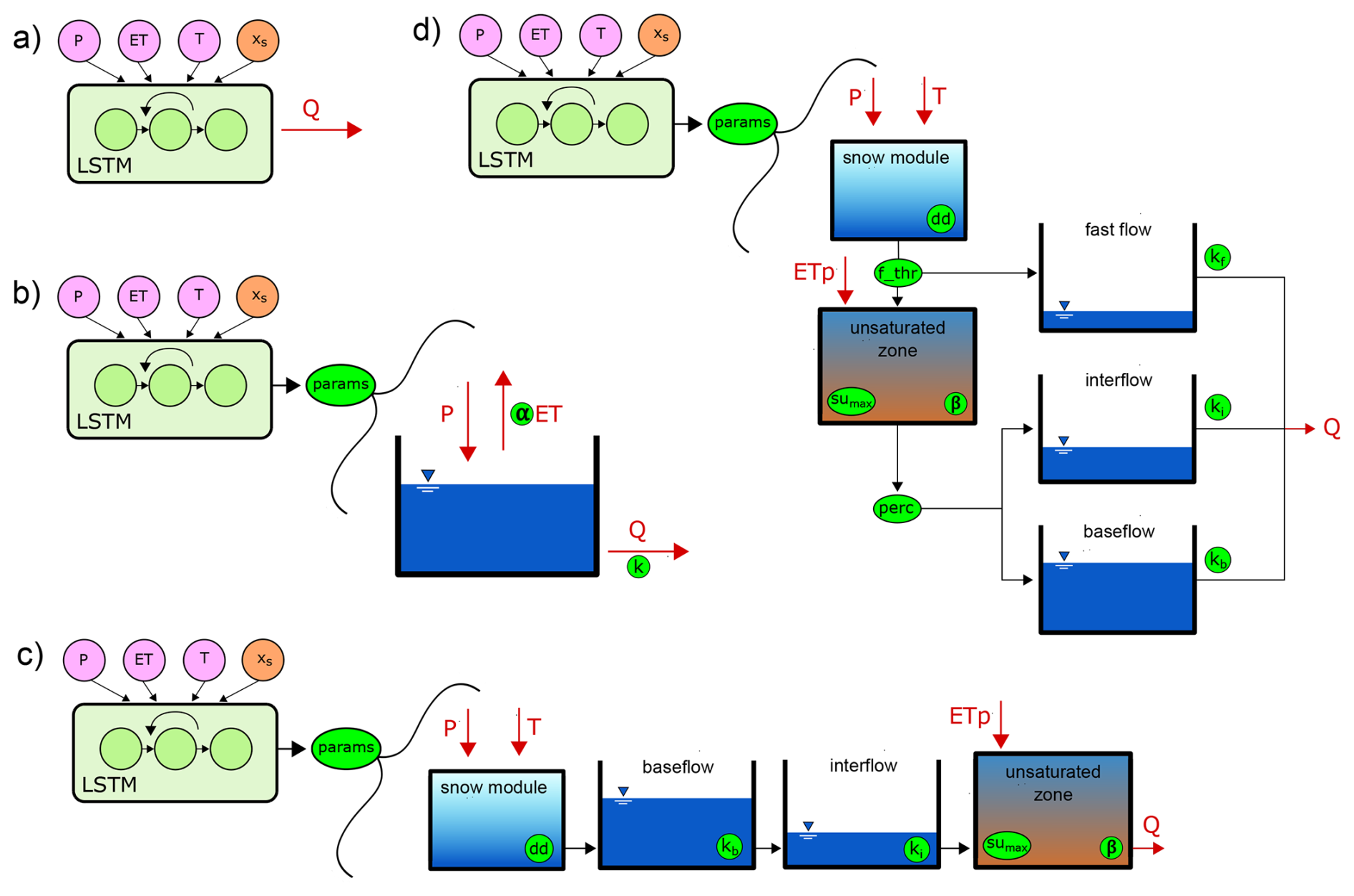
Figure 1Sketch of the hybrid models used in this study. The parameters in each model are encircled and highlighted in green. (a) LSTM, (b) Hybrid Bucket, (c) Hybrid Nonsense, (d) Hybrid SHM.
While SHM represents a model typically used in hydrological practice, the Bucket and Nonsense models serve as alternative hypotheses to test the limits of the hybrid modeling approach. These models were built using principles from modular frameworks that still find applications in hybrid modeling (Clark et al., 2008; Fenicia et al., 2011).
In simple terms, the approach to hybrid modeling used here can be conceptualized as a hydrological model with dynamic parameters. In rainfall-runoff modeling, the use of dynamic parameters originated with data-based mechanistic modeling (Young and Beven, 1994), which established methods for identifying time-invariant parameters in relation to their time-variant counterparts. More recent approaches generate time-dependent parameters by introducing stochastic processes that represent deviations from calibrated static parameters (Reichert and Mieleitner, 2009). In these methods, both static parameters and their variable components are jointly calibrated via Bayesian updating using Markov chain Monte Carlo. While theoretically convincing, the practical application of stochastic, time-dependent parameters has been very limited due to identifiability problems and the computational burden of propagating time-dependent parameters in a rigorous Bayesian framework (Reichert et al., 2021). With the recent gain in popularity of differentiable models, the idea of dynamic parameters (albeit in a deterministic setting) has experienced a significant revival in hydrological modeling.
At runtime, the LSTM runs for the entire length of a sequence of inputs and predicts the conceptual model's parameters at every time step. These predictions are made in “sequence-to-sequence” mode. After this initial run, the operation of the model resembles a traditional hydrological model with the distinction being that the model reads a new set of parameters at every time step along with it's inputs, therefore the parameters of the model vary in time. Due to the initial run of the LSTM and the warm-up period of the hydrological model, all hybrid models in this paper use a sequence length of 730 d (2 years) with only the second half of the predictions (ysim) evaluated in the loss function. Furthermore, instead of evaluating the model at each unique selection of 365 time steps, we limit the number of evaluations to 450 chosen randomly, meaning that the loss function is calculated using values of ysim and yobs. For more details of the evaluation process, please refer to Acuña Espinoza et al. (2024).
2.2.3 Performance evaluation
Hybrid models are typically trained to make deterministic predictions. Therefore, depending on the case, we use either the mean-squared error (MSE) or the basin average Nash-Sutcliffe efficiency (NSE*) (Kratzert et al., 2019c) as loss functions to evaluate the simulations of our model ysim with the observed data yobs.
In Eq. (3), i identifies the predictions and observations on a specific day and N the number of days over which to calculate the loss function. In the case of NSE*, B is the number of mini-batches in a training batch (typically 256) and the additional term sb in Eq. (4) represents the standard deviation of the streamflow time-series of the basin b and ϵ is a numerical stabilizer added for cases where sb is low.
2.3 Entropy-based measure of LSTM-induced parameter variability
For our evaluation, we aim to measure how much the LSTM makes the conceptual model's parameters vary over time to achieve an optimized performance during training. The underlying premise is that, when using a perfect model, constant true parameter values can be found during optimization, and the “LSTM-induced variability” will be zero. If the conceptual constraint is sufficiently honored by the LSTM, we expect a mild or null variability in the predicted timeseries of parameter values. In contrast, if a severely wrong representation of the true system is used as conceptual model, the LSTM will compensate through highly time-dependent parameter values, and the variability in parameters will be high.
This analysis can also be extended to the hidden states of the LSTM network itself. As examples, in Sects. 3.3 and 4.3, we examine cases where this extension is necessary to compare models with different numbers of parameters. In Sect. 4.5 we also look at models with different numbers of inputs.
Although there are several measures of variability, we choose to measure this variability through entropy, as it does not require any assumptions about the type or shape of the statistical distribution of the analyzed data. For analyzing the entropy of timeseries data, we have to evaluate continuous (differential) entropy (Cover and Thomas, 2006; MacKay, 2003) as shown in Eq. (5) with p denoting probability density functions (PDFs) of a random variable X with support 𝒳.
Beirlant et al. (1997) provide a comprehensive overview of different common approaches to estimating differential entropy from data. In this study, we will use the method proposed by Kozachenko and Leonenko (KL) based on nearest neighbor distances (Kozachenko and Leonenko, 1987) shown in Eq. (6):
where ψ is the digamma function , N is the number of points in a sample, k is a hyperparameter specifying the number of nearest neighbors used in the estimate, c1(d) is the volume of a d-dimensional unit ball, d is the number of dimensions of the data and is the distance between xi and its kth nearest neighbor. The KL estimator for entropy has been shown to be accurate even for data in higher dimensions (Álvarez Chaves et al., 2024) and was implemented as part of the https://github.com/manuel-alvarez-chaves/unite_toolbox (last access: 20 January 2026), a suite of tools we have developed for practical applications of information theory in model evaluation, which can be found in the code availability section of this article.
2.4 Diagnostic routine to evaluate hybrid model structure
Analyzing the variability in parameter or hidden-state space highlights cases where the prescribed conceptual constraint fails to accurately reflect the underlying system dynamics. Such discrepancies fall into two categories: cases where the physics are appropriate but other reasons make the model struggle (e.g., biased or highly uncertain input data), and cases where the physics constraint itself is problematic (e.g., due to neglected or misrepresented processes). To distinguish between these cases and gain insights into system understanding and model development, we propose a tailored diagnostic evaluation routine that scrutinizes the joint behavior of the LSTM-learned parameters. We demonstrate the effectiveness and diagnostic capabilities of this approach through didactic examples in Sect. 3.
3.1 Motivation
Synthetic examples here serve to create intuition about the role of the data-driven component in hybrid hydrological models. Specifically, we will demonstrate the role of LSTMs predicting time-variant parameters of conceptual hydrological models. We aim to answer the following questions:
-
How does the data-driven component behave in presence of a perfect conceptual constraint (i.e., the physics of the data-generating process are fully reflected in the conceptual model)?
-
How much variability in the LSTM-predicted parameter values will be detectable if the conceptual constraint is reasonable, but not a complete representation of the data-generating process?
-
How will the data-driven component react if the conceptual constraint is not reflecting the data-generating process at all?
Specific details for the experimental set up of these didactic examples are described in Appendix A1. The main point to highlight here is that all models were trained using mean-squared error (MSE) as the loss function (Eq. 3). The reason is that the data used for yobs was created synthetically by running an initial “true” model; therefore, there was no need to account for differences in the magnitude of the streamflow signals between basins.
As stated in Sect. 1.1, the main principle driving conceptual hydrological models is the conservation of mass in different reservoirs or storages within a model. Following Eq. (1), in a simple case of one storage, conservation of mass can be written as , with P being the input (precipitation) and ET and Q being two outputs (evapotranspiration and output streamflow, respectively). Let us assume a model that represents a typical power reservoir in which the storage-outflow relationship is described by the power function , where β and k are model parameters with an additional parameter α being used as a correction factor for the output flux of ET. This model and its governing equations are shown in Fig. 2a. Using the precipitation and evapotranspiration time-series of a subset of basins in CAMELS-GB (cf. Sect. 2.1) and parameter values α=0.8, β=1.2, k=24.0, we create a synthetic “observed” streamflow time-series that is shown across all plots in Fig. 2 (subplots b, d, f, i, l and o). This initial model is considered our “synthetic truth” because it was used to generate the target data (“observed” streamflow) for the competing formulations of hybrid models described in Sect. 3.2.
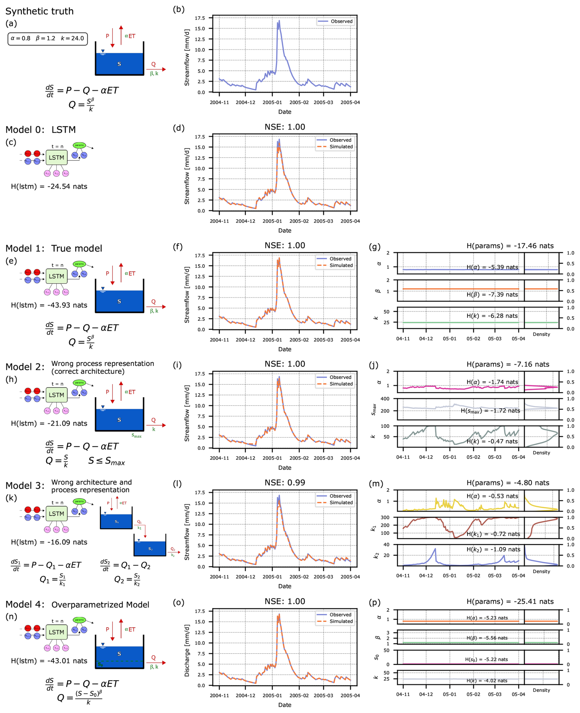
Figure 2Didactic examples, demonstrating the evaluation of hybrid hydrological models by measuring the entropy of the model parameters and the LSTM hidden-state space. Left column: Schematic illustration of hybrid model structures, with Model 1 representing the “true” conceptual physically constrained model coupled with the LSTM as a reference. Center column: Segment of observed/predicted discharge time-series. Right column: Time-series of LSTM-predicted parameters and their univariate distributions.
We will analyze the resulting time-varying parameter values of the alternative hybrid models, as predicted by their respective LSTM-component, and interpret these results given our knowledge of the true model structure in Sect. 3.3.1. Then, we will explain how we measure variability as the entropy of the resulting parameter distributions in Sect. 3.3.2, and why we move to measuring the “activity” of the LSTM in its hidden state space in Sect. 3.3.3. We summarize the key points of our proposed approach, as illustrated on these didactic examples, in Sect. 3.4.
3.2 Hybrid models
To investigate the three research questions posed above, we setup an LSTM model as our data-driven benchmark and four alternative hybrid models to predict the time-series of observed discharge, illustrated in the left column of Fig. 2:
-
We use an LSTM to directly predict streamflow from the inputs of precipitation and evapotranspiration (Model 0);
-
We couple the “true” model defined above with an LSTM network to predict its parameters α, β and k, as described in Sect. 2.2.2 (Model 1);
-
We substitute the power-reservoir with a linear reservoir that follows the storage-outflow relationship , and add a threshold parameter Smax such that any excess storage directly becomes streamflow if S≥Smax (Model 2);
-
We add an additional reservoir to Model 1 which receives the outflow of the previous reservoir and both reservoirs have a linear storage-outflow relationship (Model 3);
-
We extend the storage-outflow relationship of Model 1 with an additional threshold parameter S0 that reflects the minimum storage required to generate streamflow (Model 4).
In Fig. 2: Model 0 represents a case where we only have an LSTM which predicts streamflow, i.e. a purely data-driven model. Then, based on the distinction between structures and processes, we have categorized each hybrid model according to its architectural design and process representation. Model 2 maintains the correct one-reservoir architecture of the true model but implements an incorrect process representation by substituting the true exponential outflow relationship with a simple linear relationship. Model 3 deviates from the true model in both aspects: it uses the same incorrect linear outflow relationship while also incorporating an additional storage reservoir that doesn't exist in the true model. Model 4 preserves the correct architecture of the true model but becomes overparameterized in its process representation by introducing an extra parameter, S0. Interestingly, when S0 is set to zero, Model 4's process representation perfectly aligns with the outflow relationship in the true model. We explore these relationships further in Sect. 3.3.1. Additional exemplary model architectures are presented in Appendix B.
The LSTM architecture of the baseline model and the hybrid models consists of ten hidden states. For our entropy analysis of the hidden states to be meaningful and fair, it is important to compare models with the same architecture. The choice of ten hidden states was determined by the minimum required for both the baseline model and hybrid models to achieve equal performance. To aid in this process, the models were trained on a subset of five randomly selected basins (76005, 83004, 46008, 50008, and 96001) from the CAMELS-GB dataset. In general, using multiple basins improved the training process for all models, particularly for the pure LSTM (Model 0), validating current standard practices (Kratzert et al., 2024). However, the purpose of this analysis was not to achieve maximum performance for a given task but to compare hybrid approaches on equal grounds. We base our entropy analysis on equal performance to ensure fair statements about the role of the conceptual component in hybrid models. Additionally, to allow for extensive repetitions and alterations, we deliberately kept the training effort low (unlike the real-world case study; see Sect. 4).
The selection of these specific basins for this example is not critical. In our true model, we have defined a data-generating process that does not consider basin-specific characteristics, meaning that the models could be trained on any set of basins. The only requirement is that basins have sufficiently long time series of precipitation and evapotranspiration data, which is satisfied by all CAMELS-GB basins. We used only the precipitation and pet time series from each basin and created our own synthetic “observed” streamflow as described in Sect. 3.1 for model training. The train/test split followed the approach detailed in Sect. 2.1. Parameter variation ranges for the conceptual model components are shown in Table A1. Since the target is the product of a model, there was no need to adjust the loss function for specific data characteristics; therefore, we chose MSE (Eq. 3) as the loss function. Each model was trained for a specific number of epochs using model-specific learning rates. We refer readers to the synthetic example logs for detailed specifications of each model. The reported testing metrics are averaged over five realizations of each model obtained from random initializations using different seeds.
3.3 Analysis and discussion of results
3.3.1 Visualization of time-varying parameters
For illustration purposes, we show a short five-month period (November 2004 to April 2005, Cumbria and Carlisle floods of 2005 in the UK (Harper, 2015)) in Fig. 2 to demonstrate the ability of all models to perfectly fit the data both during high and low flow conditions. The center column shows the predicted streamflow by an exemplary run of the hybrid model, and the right column shows the corresponding parameter trajectories. The reported numerical values of NSE and entropy are for the whole testing period of 1 January 1998 to 31 December 2008, and averaged over the five runs based on different random seeds for initialization. The density plots in the right column of Fig. 2 were created using a kernel-based estimate for density (Waskom, 2021), but the reported individual entropies of each parameter and the joint entropy of the model parameters were calculated using the KL estimator described in Sect. 2.3.
Pure LSTM (Model 0). For this case we see that the pure LSTM is able to make accurate predictions, perfectly fitting the observed data. As such, this model serves as our baseline and any additional knowledge should make prediction easier (reduce entropy) or more difficult (increase entropy).
Perfect physics constraint (Model 1). In the case of Model 1, where the LSTM is coupled to the true conceptual model, we hope to see that the data-driven component does nothing, i.e., it doesn't interfere with the perfect representation of the natural system that is provided by the conceptual constraint. Indeed, we find that the network predicts practically static parameters as shown in Fig. 2g, with almost negligible deviations only resulting from the effect of the sequential nature of the LSTM. Reassuringly, the LSTM is able to recover the true parameter values of α=0.8, β=1.2, and k=24.0. As a logical consequence, this hybrid model is able to perfectly mimic the observations with an NSE of 1.0, as they were created with the same conceptual model and parameter values.
Imperfect physics constraint (Models 2 and 3). The behavior of the time-varying parameters is expected to differ when the LSTM is coupled to a conceptual model that does not adequately represent truth. Subplots (j) and (m) of Fig. 2 illustrate the behavior of the parameters when the conceptual component of the hybrid model has been incorrectly specified. In these cases, we can see how the LSTM varies the parameters in order to achieve good predictions despite an imperfect conceptual model (i.e., the LSTM compensates for model structural error). This behavior is apparent in the variation of the recession constants for Model 2 (k) and Model 3 (k1 and k2). In situations of low flow, the recession constants increase, whereas for situations of high flow, the reverse is true.
Over-parameterized constraint (Model 4). In the case of an over-parameterized conceptual model, the role of the data-driven component is somewhat unclear. All parameters might be tweaked simultaneously in a manner that changes over time, to achieve a best-possible fit with the observed data. Such a case would presumably spoil any attempts to interpret the inner functioning of the hybrid model. However, in this case, we observe that the parameters of Model 4 (Fig. 2p) are optimized to have almost constant values. In fact, the LSTM is able to correctly identify that the threshold parameter S0 is not meaningful in predicting the output variable, so it is efficiently driven to a value of 0.0. By doing so, the LSTM transforms the prescribed constraint in the form of the over-parameterized conceptual model into an architecture that is equivalent with the true one. This allows the LSTM to identify the true values of the other three parameters.
In Appendix B, we present four additional hybrid model versions that cover one under-parameterized case (Model 5 lacks the parameter β), and three over-parameterized cases of different types (concerning model structure and parameters). The insights from these scenarios match what we have reported for the three broad classes above: the under-parameterized model struggles with the effect that parameters are heavily varied, while the LSTM in over-parameterized models produces almost static parameters in a combination that counteracts the over-parameterization best.
3.3.2 Measuring entropy of conceptual model parameter space
To quantify the variability of LSTM-predicted parameter values over time, we aggregate all individual values into a sample. These samples are shown as distributions in subplots (g), (j), (m) and (p) of Fig. 2. Wide distributions result for cases where parameters vary significantly over time, and very narrow distributions for cases of almost static behavior. We can quantify the entropy of the joint distribution of the parameters by using Eq. (6) as described in Sect. 2.3, with entropy being larger for wide distributions and lower for narrow distributions. Let it be noted that we are calculating the entropy of the parameters predicted by the neural network which occupy a range of values from 0 to 1 as shown in the right-hand side of the right-most subplots in Fig. 2, such that the measurements of entropy are not affected by the scale of the parameters. Hence, these values occupy a range of values of 1, and considering that the maximum entropy (of a uniform distribution) over this value range is 0.0, the calculated entropies are negative (with more negative meaning smaller entropy which equals smaller variability).
Perfect physics constraint. Comparing the entropies obtained for Models 1, 2 and 3, we can confirm that Model 1 (LSTM coupled to the true conceptual model) shows the lowest entropy. In a theoretical ideal case, the LSTM would have been able to perfectly recover the true values of α, β and k without any variation in time at all, and that would lead to a theoretical entropy of −∞ (but this is an unrealistic expectation given the difficult task required of the LSTM, and numerical imprecisions). Nevertheless, the variations of the parameters are very small and thus also the calculated entropy is significantly smaller than for Models 2 and 3.
Imperfect physics constraint. We find that Model 2 generates less entropy than Model 3, which means that the conceptual model in Model 2 better represents the true model underlying the observed data (while definitely being further from the truth than Model 1). In this sense, the proposed entropy measure can be considered to represent “closeness” of a model's representation of the true system.
Over-parameterized constraint. Measuring the entropy of the parameters for Model 4 distorts this result. As Model 4 permits a parameter configuration that makes the model equal to Model 1, the predicted parameters of the LSTM are again almost constant, and the calculated joint entropy is even lower than for Model 1. Note that this is a special case of an over-parametrized model. In Appendix B, and particularly in Fig. B1g we show an example of an over-parametrized model in which the true model is not findable.
Comparing Conceptual Constraints on the Entropy Axis. To gain more intuition about how our hybrid models are ranked based on entropy, we place them all (including the ones presented in Appendix B) on the same entropy axis (Fig. 3).
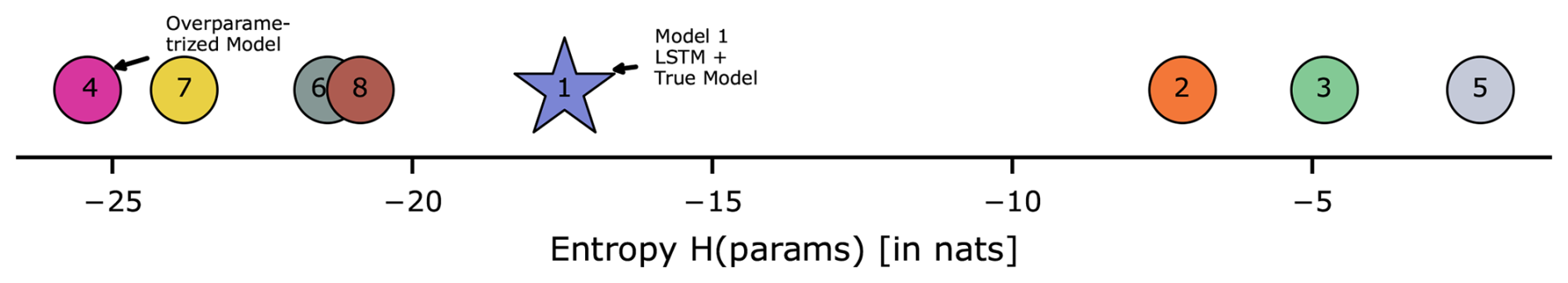
Figure 3Benchmarking axis based on the entropy of the time-varying parameters in the different hybrid models (didactic examples).
We would expect to find Model 1 furthest to the left in Fig. 3, because the LSTM has nothing to adjust, so parameters are practically constant over time and their joint entropy is minimal. However, we see that is not the case and, among the models discussed in this section, it is Model 4 which creates the lowest entropy.
This is an artifact of comparing entropies in different dimensions. As an example, consider X to be a random variable that follows a multivariate Gaussian distribution, i.e. with μ∈ℝd and . The entropy of X is then given as:
We can see that the entropy of X is directly proportional to the determinant of Σ. If we add a single dimension to Σ with a very low value on the main diagonal (a timeseries of almost-constant values will have close-to-zero variance) and all off-diagonal entries being practically zero, the value of entropy tends to decrease because the decrease of the second term through multiplication of the original determinant with a value smaller than one tends to outweigh the increase of the first term.
There are two additional cases which show lower entropy due to the number of parameters in their conceptual models (Models 6 and 8) and one further example which has entropy close to Model 4 because it shares a similar inflow-outflow relationship (Model 7). The issues with these results are explained further in Appendix B. While explainable through theory, this ranking is counter-intuitive and does not meet our expectations for a metric that unifies the evaluation of arbitrary hybrid models. We have illustrated these results here to allow the reader to follow our argument and move with us deeper into the hybrid models, i.e., into the LSTM hidden-state space.
3.3.3 Measuring entropy of LSTM hidden state space
To overcome the challenge of appropriately comparing the “activity” of the LSTM for models with differing numbers of parameters, we propose that the entropy of the coupled system should not be measured in the space of the parameters but in the space of the hidden states of the LSTM instead. Because all of the networks in this example have the same number of hidden states (10) which move in the same range of values (−1 to 1 due to the tanh function in the operations in the network), the calculated entropies will be comparable between themselves.
The entropy values obtained for the hidden state spaces of all four models are reported in the left column of Fig. 2. The hidden states of the LSTM in Model 1 have smaller variations than in the rest of the models, and thus the entropy of this network is the lowest among all candidates. This measure of variability has an even more intuitive interpretation as how much the LSTM has to compensate for a misspecified conceptual constraint.
Comparing Conceptual Constraints on the Entropy Axis. When placing the models on our universal entropy axis in Fig. 4, Model 1 now appears furthest to the left, which meets our expectation that the true constraint should coincide with minimal “activity” of the LSTM. We also see the same ranking between Model 2 and Model 3, which again makes intuitive sense, as using a one-reservoir-model better matches the true system. Finally, rearranging by the entropies of the LSTMs, Model 4 is now to the right of Model 1, which identifies it as a misspecified conceptual model, but honors that the resulting hybrid configuration is very close to the true system, as opposed to the proposed configurations in Models 2 and 3. Hence, measuring the entropy of the LSTM hidden states prevents us from disingenuous conclusions obtained by making unfair comparisons between models with different number of parameters.
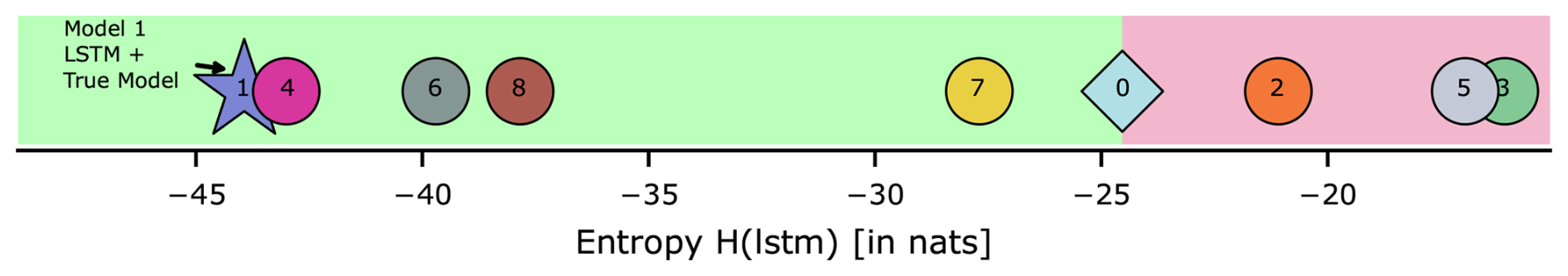
Figure 4Benchmarking axis based on the entropy of the trajectories of the LSTM hidden states in the different hybrid models and the pure LSTM (didactic examples). The division of the green and red backgrounds serves to identify the addition of “good” and “bad” constraints, respectively.
Pure LSTM as a Reference. One more advantage of measuring the entropy directly in the hidden states of the LSTM is that any hybrid model can now be compared to a single “pure” LSTM, i.e., an LSTM with a simple linear head layer instead of the conceptual model. The addition of a conceptual head layer should make the prediction task of the LSTM easier – at least this is the prevailing idea when promoting “physics-informed” ML. In our setting, adding useful information through the conceptual constraint should reduce the required activity of the LSTM, and hence, entropy. If, by contrast, the conceptual constraint made the task even more difficult, it would add entropy. Marking the pure LSTM as Model 0, we can create a divide on our axis between models that add “good” (helpful) physics (here: Models 1 and 4), and models which add “bad” (misleading) physics (here: Models 2 and 3). In addition, Models 5, 6, 7 and 8 are discussed in Appendix B, where it is shown that they also fall consistently in these categories of “good” and “bad”.
On the Complexity of the Prediction Task. The LSTM by itself can be seen as a baseline of the required complexity for accomplishing the prediction task. The proposed measure of entropy can be related to the overall complexity of the network as the entropy of the trajectories of the states in dynamical systems has been related to their Kolgomorov complexity (Galatolo et al., 2010). In theory, if the true model is specified as the conceptual head layer, the entropy of the LSTM is reduced to the theoretical minimum (−∞) and the required entropy or complexity to accomplish the specific modeling task is completely contributed by the conceptual head layer. Hence, the entropy of the conceptual head layer in Model 1 should be exactly the same as the entropy of the pure LSTM (Model 0), but measuring the entropy of the conceptual head layer by itself is not straight-forward and remains an open challenge.
3.4 Summary of the proposed approach
Let us distill our proposed approach as a diagnostic framework that discerns the adequacy of conceptual constraints in hybrid models. When the prescribed conceptual model accurately represents the natural system, the LSTM will exhibit minimal intervention, effectively endorsing the conceptual model. Conversely, when the conceptual constraint fundamentally misrepresents the system dynamics, the LSTM will demonstrate high activity, working extensively to overcome the inherent limitations of the prescribed conceptual model. This difference in LSTM activity serves as a clear signal for assessing the fidelity of our initial conceptual model.
These situations can be detected by the following proposed workflow:
-
Visualize the time-sequence of LSTM-predicted parameters to gain insight about how heavily the data-driven component acts against the physics constraint; draw conclusions about compensation mechanisms and judge whether the physics constraint is sufficiently honored or massively altered in the hybrid model.
-
Quantify the joint entropy of the LSTM hidden state space trajectories; compare against a pure LSTM for the prediction task for reference, and, ideally, against alternative formulations of conceptual constraints by placing all resulting entropies on the universal model evaluation axis.
-
Interpret the results: are the conceptual components of the hybrid models an advantage or a burden in solving the prediction task? Which configurations are more helpful than others? Try to understand why from step 1. Over-parameterization will tend to be helpful but with some parameters driven to “unphysical” values; under-parameterization will make the task unnecessarily difficult.
From the analysis of the didactic examples, we specifically want to highlight that the constraint-morphing capability of the data-driven component is both an opportunity and a risk: it is very promising to see that the flexibility of the LSTM is not abused, but rather it points us towards parsimonious model structures (as in Model 4). At the same time, this constraint-morphing happens under the hood (e.g., resulting NSE is practically the same for all our analyzed model versions!) – it is not safe to say that a hybrid model naturally satisfies the constraint we have prescribed. As such, we should be careful with stating that a model is “physics-constrained” before investigating in detail what the final version of the LSTM is doing. This is where our proposed diagnostic routine helps.
Even though in this section we focused on cases of equal performance, in Sect. 4 and more specifically Sect. 4.3.3 we analyze a case study with real data where no true model exists and our proposed hypotheses for hybrid models yield different results in terms of both predictive performance and entropy. It is also important to note that the issue of uncertainty is not addressed by these synthetic examples because the output of the true model, and therefore our observed data, were unaffected by noise. Our measurement of entropy could certainly be part of a larger and more comprehensive framework that includes both epistemic and aleatory uncertainty (Gong et al., 2013) and probabilistic model representations, but such a framework is beyond the scope of this article. Nevertheless, any measurement of entropy will always contain a fraction attributable to the intrinsic chaos of data, which becomes particularly relevant when transitioning from synthetic to real-world applications. Interestingly, equifinality did not pose an issue with synthetic data in our experiments, as all models achieved perfect predictive performance and the model was always identifiable under the right conditions. This matches the experience of Spieler et al. (2020). However, in real-world applications, equifinality is likely to be more pronounced due to measurement errors, incomplete observations of the system under study, and other sources of uncertainty. This issue is discussed further in Sect. 4.3.2.
Following the intuition developed by the didactic examples, we apply our developed metric to a case study in large sample hydrology using the CAMELS-GB dataset.
Both the pure LSTM and the LSTMs coupled with the conceptual models have 64 hidden states each, which makes them directly comparable between themselves. All models were trained using the Adam optimizer (Kingma and Ba, 2017) with a learning rate of and a different number of epochs depending on the model, with the number of epochs always ranging between 28 and 32. The ranges allowed for the parameters of the conceptual models are listed in Table A2, the static attributes used as input to the LSTM in all models are listed in Table A3.
Further details about the study setup are presented in Appendix A2 but this analysis follows the results from Acuña Espinoza et al. (2024), so we first summarize their main findings to put these new results into context. The meticulous reader will notice some differences in the results between the previous study and these current results. These differences are discussed in Appendix C and do not impact the main findings in either study.
4.1 Motivation or: why do we want hybrid models?
Hybrid models have demonstrated significant improvements in hydrological predictions across multiple applications. These include enhanced accuracy in daily streamflow prediction (Jiang et al., 2020; Feng et al., 2022), better predictions in large basins (Bindas et al., 2024), and more precise estimates of variables like volumetric water content (Bandai et al., 2024) and stream water temperature (Rahmani et al., 2023), as some examples. In each case, the hybrid approach outperformed traditional physics-based conceptual models, including the EXP-Hydro and HBV models, the Muskingum-Cunge river routing method, and a partial-differential-equation-based description of the physical process, respectively. However, while these improvements are of note and leaving aside aspects of lacking interpretability, the central question of “to bucket or not to bucket” was: given the remarkable success of purely data-driven approaches, is the additional effort of combining them with conceptual models actually worth it?
Acuña Espinoza et al. (2024) conducted a model comparison study that evaluated four different approaches: a purely data-driven LSTM and three conceptual hydrological models, each later transformed into hybrids through the process described in Sect. 2.2.2. The three conceptual models: SHM, adapted from Ehret et al. (2020), Bucket, and Nonsense represent different hypotheses of the hydrological system. Among these, SHM is a conventional hydrological model suitable for practical applications, while Bucket and Nonsense serve as contrasting cases: Bucket being an oversimplified representation and Nonsense incorporating physically implausible assumptions.
We evaluate the streamflow prediction performance of these seven models using the Cumulative Density Function (CDF) to aggregate model performance across all 671 basins in the dataset. Figure 5 presents these results, while Table 1 provides key metrics derived from the CDF analysis. The two considered metrics are the median NSE, which corresponds to the CDF's middle quantile (the higher the better), and the “area under the curve” (AUC). The AUC serves as a summary metric where lower values indicate better performance, because the AUC becomes minimal if NSE only takes on maximum values (Gauch et al., 2021).
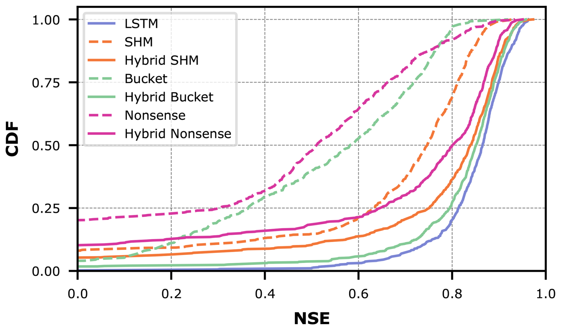
Figure 5Comparison of model performance between conceptual models with static parameters (dashed lines), hybrid models with dynamic parameters (solid lines), and the pure LSTM for all CAMELS-GB basins.
Table 1Comparison of model performance quantified by area under the NSE curve (AUC) and median NSE.
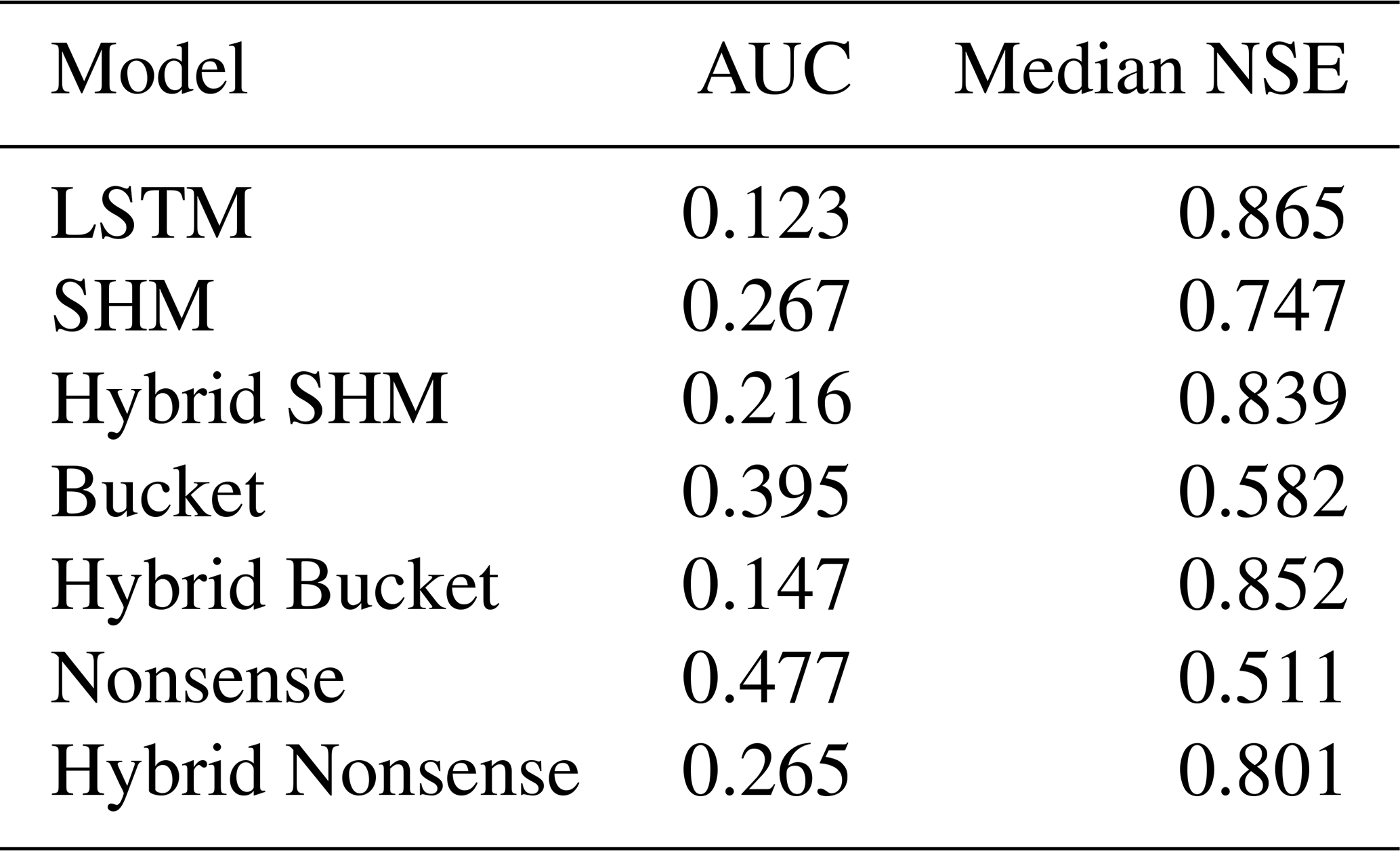
Figure 5 demonstrates the effect of combining conceptual models with LSTM networks. The effect is visible as a drastic shift to the right from the dashed lines (purely conceptual models) to the solid lines (their hybrid counterparts). This improvement is further quantified in Table 1, where the metrics consistently show improved performance for hybrid versions compared to their original counterparts.
Despite these improvements, our results show that incorporating conceptual models did not exceed the performance of a pure LSTM approach (in Fig. 5, the LSTM appears farthest to the right). Interestingly, performance improves most when hybridizing the oversimplified Bucket model, and this hybrid model matches the LSTM performance most closely. Intuitively, one might have expected the LSTM's flexibility to help the Nonsense model most, followed by the Bucket model, and finally the SHM model. Furthermore, one might have expected that after hybridization, the Hybrid SHM would perform best and exceed the pure LSTM. Instead, what we observe suggest that the SHM constraint actually limits hybrid performance, adding a Bucket-type constraint is more successful, and that none of these constraints improve prediction skill over the LSTM baseline.
These findings raise several urgent questions:
-
Why do apparently “bad” physics allow for better hybrid performance than “good” physics?
-
What can we conclude from hybrid performance after all if it does not reflect process fidelity?
-
Do physics get in the way of successful data-driven modeling?
We note that one untouched advantage of the hybrid approach lies in its ability to directly derive unobserved variables, such as soil water equivalent (SWE), without requiring secondary models. Hence, we wish to provide modelers with tools to obtain satisfying answers to these questions and to better inform and justify hybrid modeling in future research and practice.
4.2 Performance on individual basins
To better understand the mechanisms of these hybrid models and their impact on model performance, we will investigate the prediction task for five individual basins in detail. These five basins were carefully chosen to facilitate discussion in this section, as they demonstrate cases in which all hybrid models achieve similar performance (as in Sect. 3) while having different rankings based on our proposed entropy metric. In Sect. 4.3.3 we draw statistical conclusions about the prevailing behaviors for all basins.
Figure 6 exemplarily shows five basins where the performance gap between hybrid and non-hybrid versions is again very clear. However, these basins all share the characteristic that all models, including the deliberately implausible Nonsense model, reach very similar performance when hybridized. This seems counterintuitive in several aspects and again supports the research questions we have formulated above, as we would have expected to see differences in performance among the hybrid models depending on the constraints imposed. Does the LSTM truly not care what the conceptual constraint is as it can effectively transform any constraint into the same end product?
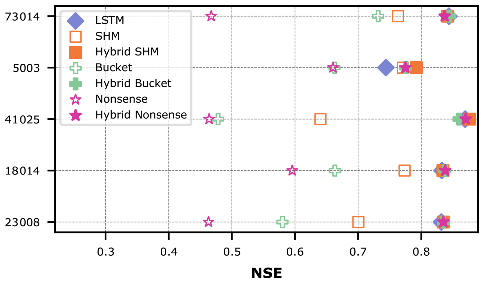
Figure 6Comparison of model performance between conceptual models with static parameters, hybrid models with dynamic parameters, and the pure LSTM for individual CAMELS-GB basins.
Furthermore, we would have expected (hoped?) that at least the physics-plausible constraint of SHM would have helped solve the prediction task, yet this is only marginally true for basins 5003 and 41025, which show slightly higher performance for the Hybrid SHM model. Confusingly, in the specific case of basin 5003, all constraints (physics-plausible or not) seem to help. Overall, Fig. 6 highlights the urgent need for diagnostic analysis tools that help us understand what it actually means to constrain a data-driven model with a conceptual hydrological model and how much physics remain inside.
Since we are in a real-data setup now, there is no “true” model or constraint that we could use as a reference for minimal entropy on our evaluation axis. We will therefore seek the LSTM component that produces the least entropy. Our main anchor will be the performance of the pure LSTM, dividing between meaningful added knowledge and misguided assumptions that require compensation by the LSTM.
4.3 Analysis and interpretation of entropy diagnostics
4.3.1 Measuring entropy of LSTM hidden state space
Following the intuition developed in Sect. 3, we address the questions in the previous section through an entropy analysis of the LSTM's hidden states for the prediction of the five individual basins introduced above.
Figure 7 shows the calculated entropy during the testing period for both the pure LSTM and the hybrid models. This is equivalent to the entropy axis we had introduced in our didactic examples, with the pure LSTM marking the divide between “good” and “bad” constraints. Overall, we find that the ranking varies per basin: in some cases (basins 23008, 18014, 41025), the pure LSTM shows by far the lowest entropy and hence none of the constraints can be considered useful for predicting streamflow at these basins; for the other basins, at least some conceptual constraints proved helpful, in basin 5003 even all of them.
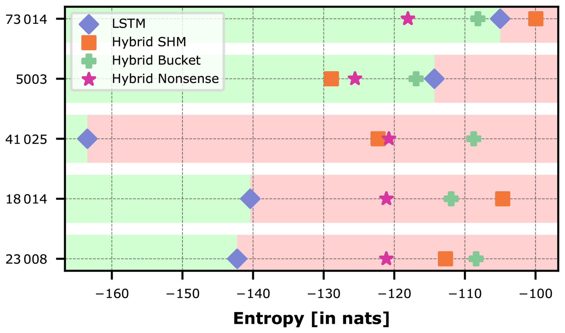
Figure 7Entropy of the trajectories of the LSTM hidden states in the different hybrid models and the pure LSTM for individual CAMELS-GB basins. The division of green and red backgrounds matches that of Fig. 4.
Focusing on basin 5003, the observed ranking aligns with our expectation that SHM is the only plausible and hence most useful constraint. This suggests that SHM's imposed structure reasonably reflects the natural system, effectively transferring part of the entropy to the physics-based component. However, any conceptual hydrological model reduces the network's entropy compared to the pure LSTM, even the Nonsense model, which opposes our expectation that this constraint should not be useful. Notably, Hybrid Nonsense shows even lower entropy than Hybrid Bucket, indicating that some complexity is necessary and a too simple conceptual model offers little benefit.
Basin 73014 presents a counterexample where Hybrid Nonsense performs best (produces the least entropy) and Hybrid SHM is located to the right of the LSTM, suggesting that a plausible hydrological model can even make predictions more difficult. This finding highlights the unpredictability of hybrid models and the need for deeper investigations to achieve interpretability; simply imposing a constraint does not do the job.
4.3.2 Visualization of time-varying parameters
In this section, we demonstrate the power of visually analyzing the time-series of the LSTM-predicted parameters on the example of exploring why the Nonsense model creates the least entropy for basin 73014. This analysis illustrates how our entropy-based metric contributes to a broader evaluation framework where models are assessed not only by quantitative metrics but also by a qualitative evaluation of their behaviour (Gupta et al., 2008).
Figure 8 (top panel) compares the differences between observed and simulated streamflow values for the non-hybrid and hybrid versions of the Nonsense model in this basin. The Hybrid Nonsense model shows drastically improved predictions, represented by the solid line in the streamflow plot, compared to its non-hybrid counterpart (dashed line). That means that allowing the parameters to vary over time greatly improves the ability of this model to make accurate predictions.
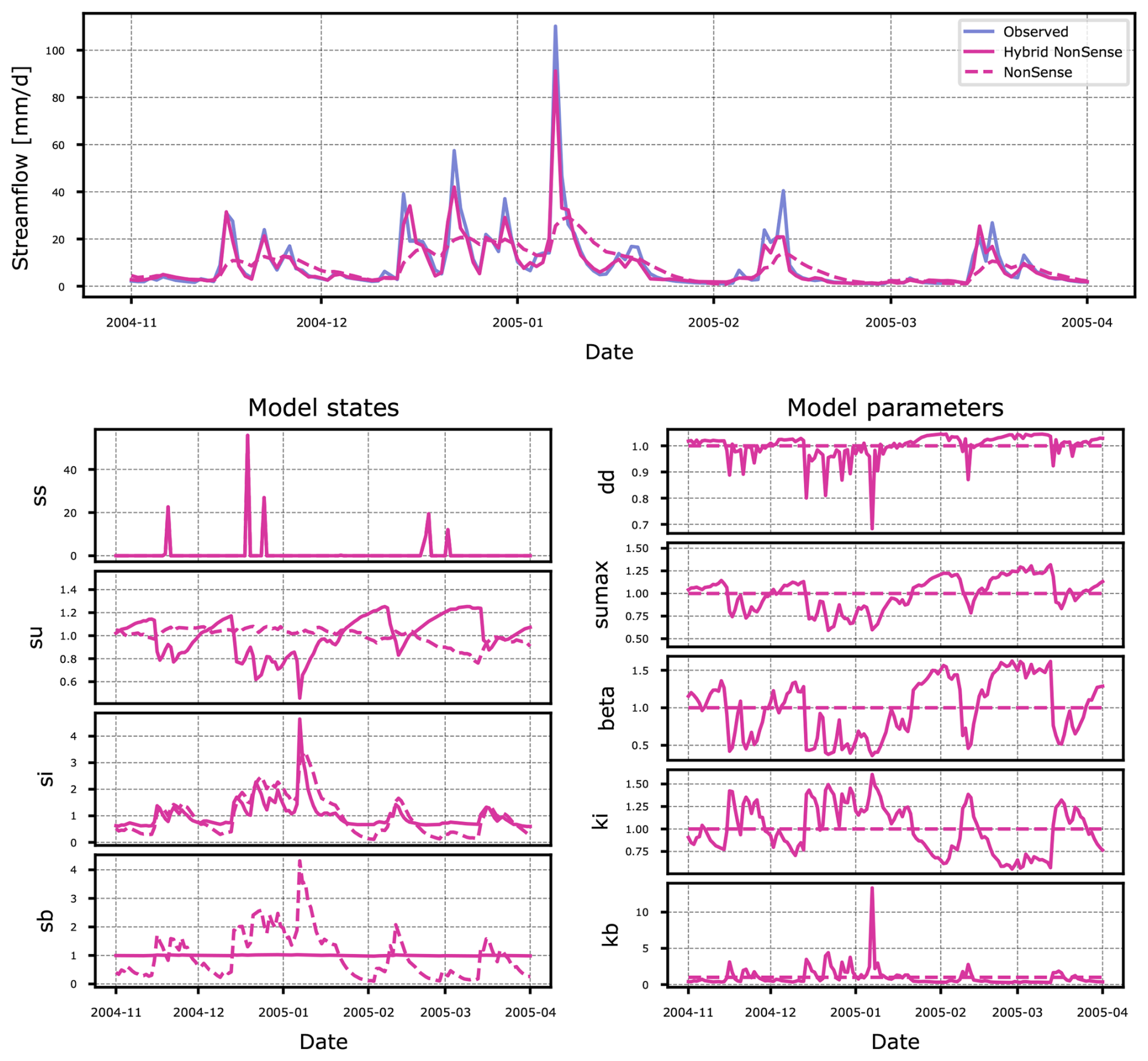
Figure 8Differences between simulated streamflow, states and model parameters of the Nonsense and Hybrid Nonsense models for basin 73014. Both the states and model parameters are shown on a scale relative to their mean.
To better understand the adjustments made by the LSTM, let us first look at the original structure of the Nonsense model, which is considered physically implausible due to the arrangement of its hydrological storage units (see schematic illustration in Fig. 1c). Counter-intuitively, water from direct precipitation or snowmelt initially enters the model through the baseflow storage, typically considered the unit with the longest retention time. The model then routes water through an unusual sequence: it moves next to the interflow storage which once again has a longer residence time, then it passes into the unsaturated zone, loses some mass through evapotranspiration, and is finally transformed into the streamflow output. Ignoring their physical interpretation for a moment, the Nonsense model basically consists of a series of three storages connected sequentially, forming a cascade-like arrangement that essentially transforms the storages into a dampening function, which delays the input signal.
The adjustments made to this implausible model structure by the LSTM component of Hybrid Nonsense become apparent when examining its states and parameters (bottom left and right panel in Fig. 8). To simplify interpretation, all plots have been normalized by the mean value of the corresponding state or parameter over the analyzed period. This normalization sets the mean value to 1.0 on the plot, with the lines indicating deviations from the mean. However, that doesn't mean that parameters for Nonsense and Hybrid Nonsense have similar or even values that are close to each other. For example, the value of su,max for Nonsense is 398.6 mm while the mean value for Hybrid Nonsense is 83.5 mm. This reflects a typical behaviour in these hybrid models were the parameters for the non-hybrid and hybrid model can occupy drastically different ranges.
Analyzing the static parameters in the Nonsense model, the dampening behavior of the storages becomes evident: the dashed lines for the baseflow storage sb and the interfow storage si closely resemble the output hydrograph, but are dampened too strongly in the unsaturated zone storage su. However, this behaviour changes significantly when the model becomes Hybrid Nonsense. Specifically, the line for sb becomes horizontal, indicating that the parameter kb is being used to effectively “skip” this storage. In fact, the Hybrid Nonsense model modifies su and si to behave as time lags for the input rainfall to become outflow which ultimately is mostly managed by the interactions between sb and kb. In Fig. 8 we see that for the high flow peak that happens in 2005-01, kb is increased disproportionately just so that the model can match the peak based on the volume available in sb.
The solid lines for su and su,max reveal a distinct pattern in which su,max closely tracks the value of su. This behavior is tied to the conditional property of the storage: if , any excess runoff added to su is immediately outputted. Because su,max consistently mirrors su, any additional runoff into this storage is immediately converted to simulated streamflow, once again, effectively bypassing this storage. In addition, the outflow of su is also managed by β which appears to be anticorrelated with si/ki to match the shape of the observed hydrograph. As a result, the Hybrid Nonsense model essentially functions as a single-storage system with added lagging behavior. This lag is introduced by the sequential transfer of mass between the storages, which occurs one at a time during each time step.
The imposed structure of the original Nonsense model was effectively modified by the LSTM, transforming the overcomplicated but physically implausible model into something that more closely resembles the Bucket model, with some additional flexibility guided by the characteristics of the training data. Since we did not impose specific constraints on the storage behavior, apart from limits to the parameters, the LSTM discovered an optimized architecture that, in combination with the data-driven component, works just as well as any of the other constraints. It seems that the modified Nonsense structure is significantly more suitable than the oversimplified Bucket model, presumably because it allows for just the right amount of additional freedom. Interestingly, morphing the structure of the Nonsense constraint costs the LSTM less effort (entropy) than fighting against (arguably) more adequate but too rigid constraints such as the SHM or the Bucket conceptual models – this is important to keep in mind when interpreting the results of our entropy analysis. High entropy clearly indicates struggling caused by the imposed constraint; low entropy paired with unaffected parameters means a plausible constraint, whereas low entropy paired with suspicious time-varying patterns that alter the qualitative behavior of the states means overwriting of constraints in favor of something more efficient; something that can potentially still be meaningful, as we have uncovered here, and also from the over-parameterization cases in our didactic examples (so, there is hope).
Figure 9 presents the same analysis period for the SHM and Hybrid SHM models in basin 73014. Due to its larger structure, interpretation becomes more challenging, but we observe some of the same behaviors identified in the analysis of Hybrid Nonsense. The LSTM determines that some of the additional storage compartments in SHM are unnecessary, as it does not utilize sb and instead regulates outflow through the fast-flow (sf) and si storages. Furthermore, minimal changes in si suggest that most of the outflow is directed through sf.
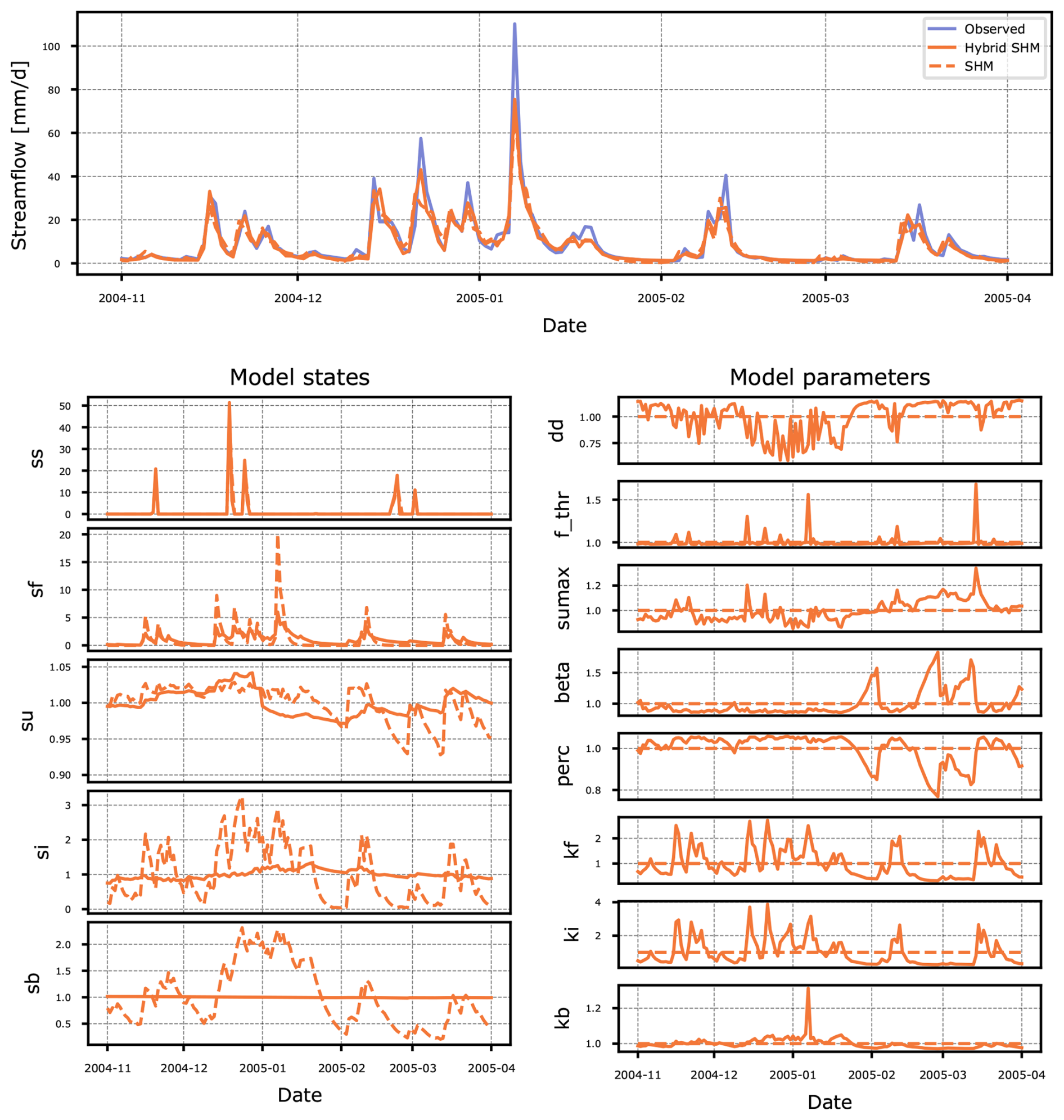
Figure 9Differences between simulated streamflow, states and model parameters of the SHM and Hybrid SHM models for basin 73014. Both the states and model parameters are shown on a scale relative to their mean.
The high variability in the LSTM-controlled parameters for the remaining reservoirs may show a learned behavior from other basins in the dataset. Such adaptation appears unnecessary for this particular basin, as the predictions made by the non-Hybrid SHM model were already sufficiently accurate and modifications made by the LSTM improved performance only slightly. Ultimately, this leads to the Hybrid SHM model being penalized, placing it last in our ranking. As a final note, that the “intervention” of the LSTM was not obvious from comparing the hydrographs produced by SHM and Hybrid SHM and without the analysis proposed here, one would think that Hybrid SHM is a well-constrained hybrid model that respects the assumptions formulated in SHM – which is not at all the case, as we have shown here.
To return to the point of equifinality made in Sect. 3.4, as we have seen in this section, different hybrid model configurations may achieve similar predictive performance while exhibiting varying levels of entropy in the LSTM hidden state space and modifications to their internal behavior. We argue that high variability in parameter combinations represents an undesirable condition in terms of model structure specification. High entropy aligns with this perspective and, in general, entropy can be used to distinguish between equifinal models.
4.3.3 Statistical analysis of results for all basins
In the previous section, we analyzed specific results from five basins in the dataset because their results mirror those of our controlled examples in Sect. 3. We can extend this analysis to all basins in the dataset to comment on their results based solely on entropy, though we acknowledge that our constraint of equal performance in the comparison does not hold, as is clear from Fig. 5. Nevertheless, while acknowledging that this constraint is not fulfilled, the insights derived in this section are meaningful to the overall understanding of hybrid models.
One could develop a model selection criterion that considers both performance and entropy. In fact, there has been previous research on model selection considering computational complexity and model performance (Azmi et al., 2021). However, our purpose here is not to introduce a criterion for model selection but to understand the role of conceptual constraints in hybrid models using entropy as a diagnostic tool.
In Fig. 7, the most common pattern across basins is shown by basins 23008, 18014, and 41025, where the LSTM consistently has the lowest entropy while the other hybrid models show non-consistent rankings. It appears that their ranking is determined by the specific hydrological system being modeled and the required model complexity. We therefore analyze here the overall statistics and rankings of entropy across all basins.
The violin plots in Fig. 10 show the entropy distributions of each model, with median values of −151.2 nats for the LSTM, −128.2 nats for Hybrid Nonsense, −113.1 nats for Hybrid SHM, and −111.0 nats for Hybrid Bucket. The LSTM's wider dispersion highlights the varying complexity required to model each individual basin. The fact that the LSTM is the only model to cover much of the lower entropy range demonstrates that, in most cases, introducing a conceptual constraint substantially increases the modeling challenge. This is apparent for Hybrid Bucket, which has the highest entropy distribution, meaning that such a simple conceptual constraint is not helpful in most cases and the LSTM has to make the most effort to compensate for this overly rigid constraint.
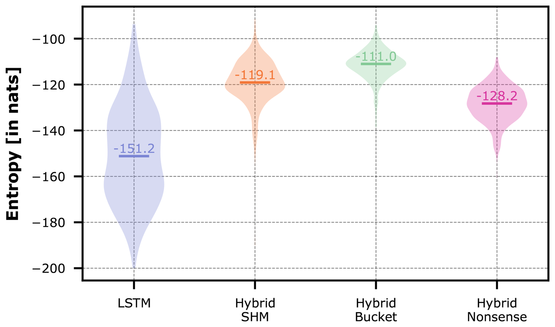
Figure 10Violin plots of the entropy of the trajectories of the LSTM hidden states in the different hybrid models and the pure LSTM across all CAMELS-GB basins.
Surprisingly, Hybrid Nonsense has the lowest median entropy among the hybrid models. This goes against an initial hypothesis that a researcher might have; yet, as our analysis in Sect. 4.3.2 has shown, the Nonsense model lends itself to being most easily transformed by the LSTM into a more suitable structure that can predict streamflow well. Finally, Hybrid SHM did not fulfill our expected result, as it seems that this model is overly complex for this specific dataset and the LSTM has more trouble using it to its advantage than the Nonsense model.
To analyze this in more detail, we collected the individual rankings per basin for the whole dataset, identified the unique rankings that appear, and determined their frequency of occurrence. The counts of rankings are shown in Fig. 11.
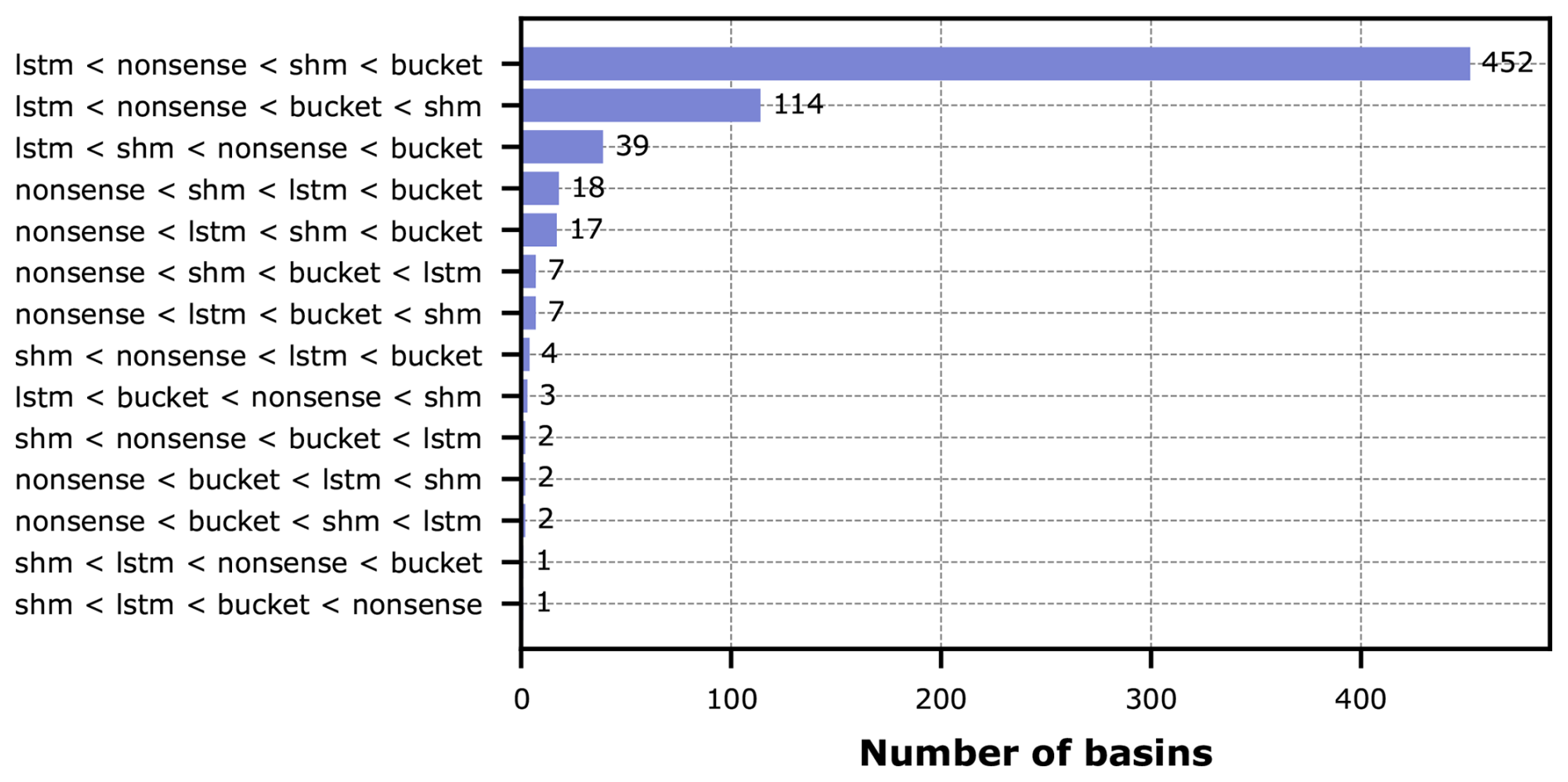
Figure 11Counts of the different entropy-based model ranking outcomes across all CAMELS-GB basins. To limit the length of the label, the shorter conceptual names of the hybrid models were used but the counts are for the hybrid versions of these models.
The ranking suggested by the medians in Fig. 10 (entropy of LSTM being lowest, followed by Hybrid Nonsense, Hybrid SHM, and Hybrid Bucket) reflects most frequent ranking across all basins (67 %). Aggregating all those basins, for which the pure LSTM obtains the lowest entropy, leads to 91 % of all basins. This tells us that, in general over this particular large-sample dataset, the conceptual representations used in our hybrid models were not able to make the prediction task easier for the LSTM and the prior knowledge that we tried to enforce didn't help. Ultimately we got a hybrid model that predicted well not because of the physical constraints that we imposed, but because the LSTM was able to compensate for these constraints through added effort (entropy).
Although our previous statement is the main finding of this study, we are still able to identify specific catchments for which the added prior knowledge indeed helped. In Fig. 11 there are 11 basins (1.6 %) which show the LSTM at the top, meaning that any of the conceptual models added information that helped in prediction; in 8 out of 671 cases (1.2 %), Hybrid SHM showed the lowest entropy, meaning that the constraint that a hydrologist would perceive as the most plausible and useful actually turned out to need the least compensation by the data-driven component. And only in 1 out of 671 cases, the physically least plausible Nonsense model needed the most compensation.
4.4 What if only individual parameters are dynamic?
Although our experimental settings have been deliberately kept consistent with Acuña Espinoza et al. (2024), it is not necessary for every model parameter to be dynamic, as in the cases examined so far, for our method to work. Rather, it could be scientifically interesting to examine the role of individual parameters in “fighting” the imposed constraints. To illustrate the diagnostic capability of the proposed entropy analysis for this question, we examine a variant of the SHM model in which only the parameter β in the unsaturated zone reservoir is made dynamic, while the remaining seven parameters remain static.
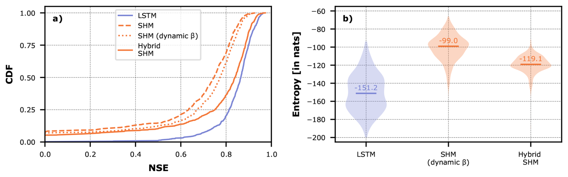
Figure 12(a) Model performance for the LSTM, SHM (all parameters static), Hybrid SHM (all parameters dynamic), and SHM β dynamic, models across all CAMELS-GB basins. (b) Violin plots of the entropy of the trajectories of the LSTM hidden states in the different hybrid models and the pure LSTM across all CAMELS-GB basins.
Figure 12a shows the NSE CDF curves for the LSTM, SHM (fully static), Hybrid SHM (all parameters dynamic), and this new SHM β-dynamic variant. The single-parameter dynamic model shows a slight performance increase compared to the fully static conceptual model, but does not match the performance of the model with all dynamic parameters.
Figure 12b presents the entropy distributions for these models. The fully static conceptual model has no entropy and therefore is not shown. Notably, the single dynamic-parameter variant exhibits significantly higher entropy than even the Hybrid SHM model with all parameters dynamic. This observation is consistent with our interpretation of entropy as a measure of LSTM activity: when the LSTM must compensate for model misspecification through only one degree of freedom instead of eight, as in Hybrid SHM, its activity (and thus entropy) increases substantially without proportional performance gains. In the SHM β-dynamic case, the LSTM attempts to correct the entire conceptual model through a single point of entry. By contrast, in the Hybrid SHM case, the LSTM makes smaller adjustments across multiple model components, resulting in higher performance and lower entropy.
This example demonstrates that entropy can serve as a diagnostic for identifying how the neural network component compensates for structural inadequacies in the conceptual model as represented by individual parameters. This suggests the possibility of systematically diagnosing individual components by selectively making parameters dynamic or static, with entropy guiding the process toward a model representation that more realistically reflects the natural system.
4.5 What about other approaches to hybrid modeling?
Measuring the entropy of the data-driven component of a hybrid model works particularly well in our setup because of the tight coupling between the LSTM and the conceptual hydrological model through the parameters of the latter. Nevertheless, our suggested approach can be effectively applied to other types of hybrid models or physics-informed machine learning.
As one example of an alternative approach to physics-informed machine learning, post-processing the results of a hydrological model to improve its predictions has been suggested (Nearing et al., 2020; Frame et al., 2021). For this application, a traditional hydrological model with static parameters makes an initial run to predict streamflow, and the predictions as well as the states of the hydrological model are fed to an LSTM to make improved predictions of streamflow. The approach is successful in the sense that it improves predictions of streamflow and manages to move all performance CDF curves close, but not beyond, the LSTM as shown in Fig. 13. Note that both the LSTM and post-processing LSTMs use the same number of hidden nodes (64), making our approach and comparison still applicable.
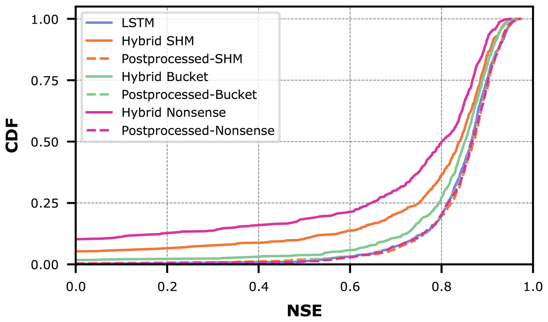
Figure 13Comparison of model performance between conceptual models with static parameters (dashed lines), post-processing hybrid models with dynamic parameters (filled lines), and the pure LSTM for all CAMELS-GB basins.
The violin plot of entropies for the LSTM hidden states across all basins shown in Fig. 14 suggests a different conclusion than for our previous hybrids. It seems that the LSTM is largely “unimpressed” by the additional input, no matter which model it was created by; only the Nonsense model (of all things!) seems to be able to effectively reduce the effort required for the prediction task, meaning that there is some pre-processing that this particular model does that is actually helpful. Figure 15 shows a much more mixed bag of results where, for certain specific basins, any of the conceptual models might produce an output that reduces the entropy of the LSTM. Considering that feeding the model “Nonsense” is helpful in close to 80 % of all basins should again be an impressive warning that feeding physics-based model output to a data-driven model is not necessarily physically meaningful (in that case, we would expect the LSTM to have a harder time with nonsense outputs). This confirms previous findings in literature which suggest that post-processing a conceptual model is not a good method to make “physics-informed” machine learning (Nearing et al., 2020; Frame et al., 2021).
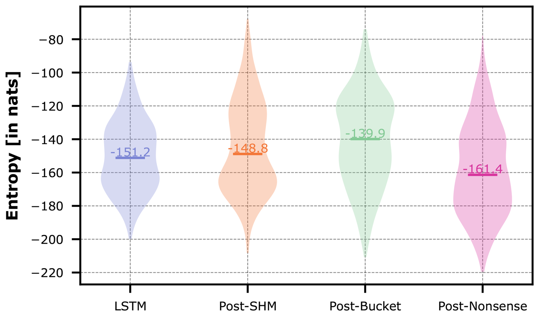
Figure 14Violin plots of the entropy of the trajectories of the LSTM hidden states in the different post-processing hybrid models and the pure LSTM across all CAMELS-GB basins.
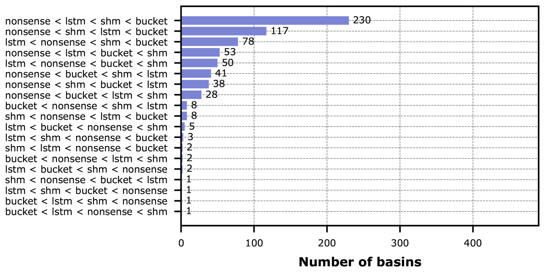
Figure 15Counts of the different entropy-based model ranking outcomes across all CAMELS-GB basins. To limit the length of the label, the shorter conceptual names of the post-processing models were used but the counts are for the hybrid versions of these models.
Since post-processing conceptual models do not allow for scrutinizing conceptual states or parameters, as with hybrid models, we cannot perform our detailed analysis as shown above (Figs. 8 and 9). Hence, interpretation of the impact of the physics-based input (hard to call this a constraint) requires interpretation of the LSTM hidden states. This is a current line of research in its own right (e.g., Feng et al., 2024b; Blougouras et al., 2024), and goes beyond the scope of this study. It will be interesting to explore what the contribution of “Nonsense” is that seems to simplify the prediction task for the LSTM, while physically-meaningful outputs as LSTM inputs do not necessarily help.
4.6 Summary of findings from the case study
In this case study, we compared a pure LSTM model with three hybrid hydrological models based on the CAMELS-GB large-sample data set. Overall, we found that the LSTM outperformed the hybrid models in predicting streamflow, and our entropy analysis revealed that adding physics-based constraints generally did not simplify the prediction task.
Our analysis also showed that the LSTM effectively adjusts the constraints imposed by the conceptual model. For instance, Hybrid Nonsense is very different from its original Nonsense formulation with the LSTM identifying an optimized architecture that, when combined with a data-driven component, performs just as well as all other models. The degree of effort required for the LSTM to modify these constraints provides insight into how accurately the conceptual model represents the underlying system. This finding highlights a key opportunity for hybrid modeling: refining existing models to better suit specific sites based on training data characteristics. In essence, hybrid models can guide us toward more parsimonious model structures.
Notably, this process occurs entirely under the hood. If we had evaluated performance using only NSE, we might have mistakenly concluded that the Nonsense constraint was just as valid as SHM or Bucket, since all three achieved the same performance when paired with the LSTM. These results overwhelmingly suggest that we need to reconsider our ways of building and evaluating hybrid models. Even if “just” the parameters of conceptual hydrological models are modified by the data-driven component, the resulting hybrid models function differently than what we expect by imposing mass balance equations.
While our findings might be specific to the particular dataset and model candidates used in this study, we have provided an objective method to test our hypotheses in arbitrary other scenarios. Future research should explore a wider range of datasets and hybrid model architectures to validate and extend our conclusions.
Finally, we have provided an outlook of how to apply our entropy-based analysis to only partially-dynamic hybrid models and even other types of hybrid construction. While there are differences between approaches that should be taken into consideration for an in-depth analysis of architectures, the evaluation of entropy in the LSTM hidden states already provides an objective insight that would have been obscured when only considering skill scores. Complementary analyses that target the specifics of other hybrid model architectures are left for future work.
“Man is always prey to his truths. Once he has admitted them, he cannot free himself from them” (Camus, 1991). The pursuit of a single, universal model to explain every hydrological system is fundamentally absurd. This paper challenges the hydrological community's tendency to rely on a single model, like SHM, as a comprehensive explanation for the complex dynamics of all river basins. Our work shows that SHM, or other conceptual models of its kind, is precisely the kind of rigid “truth” Camus warned us about: a single model that, now coupled with a component that learns from data, represents a seemingly straightforward explanation of every and any complex natural system.
The recognition of these limitations extends to the process of model selection itself. As observed by Kuhn and Hacking (2012), “scientists work from models acquired through education and subsequent exposure to the literature, often without fully knowing what characteristics have elevated these models to the status of community paradigms”. This implicit acceptance of certain modeling approaches, while pragmatic, further highlights the tension between using an interpretable model and capturing the full complexity of real-world systems. Hybrid models acknowledge this tension by incorporating prior knowledge to achieve partial interpretability while accepting the residual complexity that remains unmodeled. However, our study suggests that this balance is often skewed in favor of the data-driven component. The use of a conceptual model as a structural prior represents an attempt to extract meaningful dynamics from a larger environmental system (Young et al., 1996), but as we have shown, this attempt is often forced. When the problem is relatively simple, such as predicting streamflow in our case study, conceptual prior knowledge is largely ignored in favor of a more flexible, data-driven structure, raising the question of whether it was necessary in the first place if only predictive capacity is considered.
Our primary contribution is a metric that quantifies how much prior knowledge contributes compared to a purely data-driven approach. In Sect. 3, we demonstrated how different conceptual models can be evaluated based on how closely their prescribed equations align with those governing the “true” system. Our key finding was that the hybrid model containing the “true” conceptual model required the least assistance from the LSTM (lowest entropy), while models with architectures very different from the true underlying process required the most assistance from the LSTM (highest entropy). This demonstrates that our entropy metric can distinguish between conceptual models that perform well for the right reasons versus those that achieve good performance just through compensation by a data-driven component, a distinction that traditional performance metrics cannot make.
Interestingly, measuring the “complexity” of the LSTM in the sense of measuring its “compensation activity” when coupled to a parsimonious but inadequate representation yields larger entropy than when coupled to a more flexible inadequate representation. This means two things: low entropy does not automatically mean that the constraint is honored and that it is realistic; and the LSTM seems to have more work to do to fight against something simple but wrong than to fiddle around with an arbitrary, flexible enough structure to make it work. We have seen this in the overparameterization cases in the didactic examples and with the nonsense model in the case study. So, high entropy means the LSTM is struggling because of a too rigid, inadequate constraint. Low entropy means that the LSTM is seeing something in the constraint; however, deeper analysis in the form of inspecting parameter and state trajectories are required to distinguish whether the constraint is deemed reasonable to predict the data (constant parameters), or whether it just lends itself well to be transformed into something new, parsimonious, and effective, which might even be physics-explainable and guide us towards a better representation of the true model. So, there is hope in hybrids; just in a different way than the community might have anticipated.
Additionally, we showed that a data-driven model can serve as a reference point, distinguishing between conceptual models that better approximate reality and those that do not. We propose that data-driven models should serve as the baseline for evaluating hybrid models, which allows us to determine whether incorporating prior knowledge, such as physics-based constraints, genuinely enhances predictive performance or simply adds unnecessary complexity.
Applying this metric to a large-scale case study revealed that our attempts to improve predictive capacity through hybridization were often unsuccessful. This was because the added knowledge rarely captured the true system dynamics, forcing the flexible component of our models to compensate for incorrect assumptions (Sect. 4.3.2).
Beyond performance, there may be broader value of hybrid models with respect to interpretability and process fidelity. In that context, it is highly important to evaluate the degree to which physical constraints actually constrain model behavior: if the intended model structure that should guarantee interpretability is overwritten, this argument is no longer valid, or we might actually discover a better (in our case: simpler) process representation that again allows for scientific insight and learning. Additionally, correlation between a labeled storage component and external variables should not be the sole standard for evaluating hybrid models because, as we have shown, the original constraint that defined that label may no longer apply in the final model structure.
While we focus on entropy as our primary metric, we believe entropy complements, rather than replaces, other existing evaluation approaches focused on process representation and physical understanding. Furthermore, the compensation work of the LSTM should be related to aspects of achieved performance to provide a comprehensive basis for model selection, with the identification of appropriate ways to potentially combine these aspects into a single informative metric being left as an open research question.
In the future, hybrid models could become valuable tools for refining our understanding of hydrological systems, but only if we critically reassess traditional modeling practices. The fact that even a “nonsense” conceptual model demonstrated the highest potential for adding useful information in post-processing hybrids raises new questions. We hypothesize that physics constraints in the form of strict sequential processing may be too rigid and that guiding the LSTM toward learning appropriate lag functions or the entire hydrological model itself could be a more effective strategy.
Overall, our findings challenge the assumption that physics-informed machine learning necessarily preserves the physics as initially formulated. Instead, the data-driven component may restructure the imposed constraints, uncovering a more effective, potentially physics-explainable alternative. We do not oppose hybrid modeling; rather, we propose a quantitative tool to analyze how much the physics-based constraints are modified and suggest a workflow for diagnosing these structural adaptations. In the end, hybrid modeling, when paired with information-theoretic analyses, has the potential to provide valuable physical insights. Without such an approach, however, many so-called “physics-informed” models may be better described as physics-ignored.
We provide further details of our experimental setup in this section, and point the interested reader towards a repository in the data repository of the University of Stuttgart (DaRUS) that contains all the code for this project including: training scripts, logs and archived netCDF files of the saved internal and hidden states, fluxes and predictions made by each model. The repository can be found at this link: https://doi.org/10.18419/DARUS-4920 (Álvarez Chaves, 2025).
A1 Didactic examples
The ranges for the parameters of the conceptual models allowed in the didactic examples are listed in Table A1.
Table A1Ranges of the model parameters in the synthetic examples.
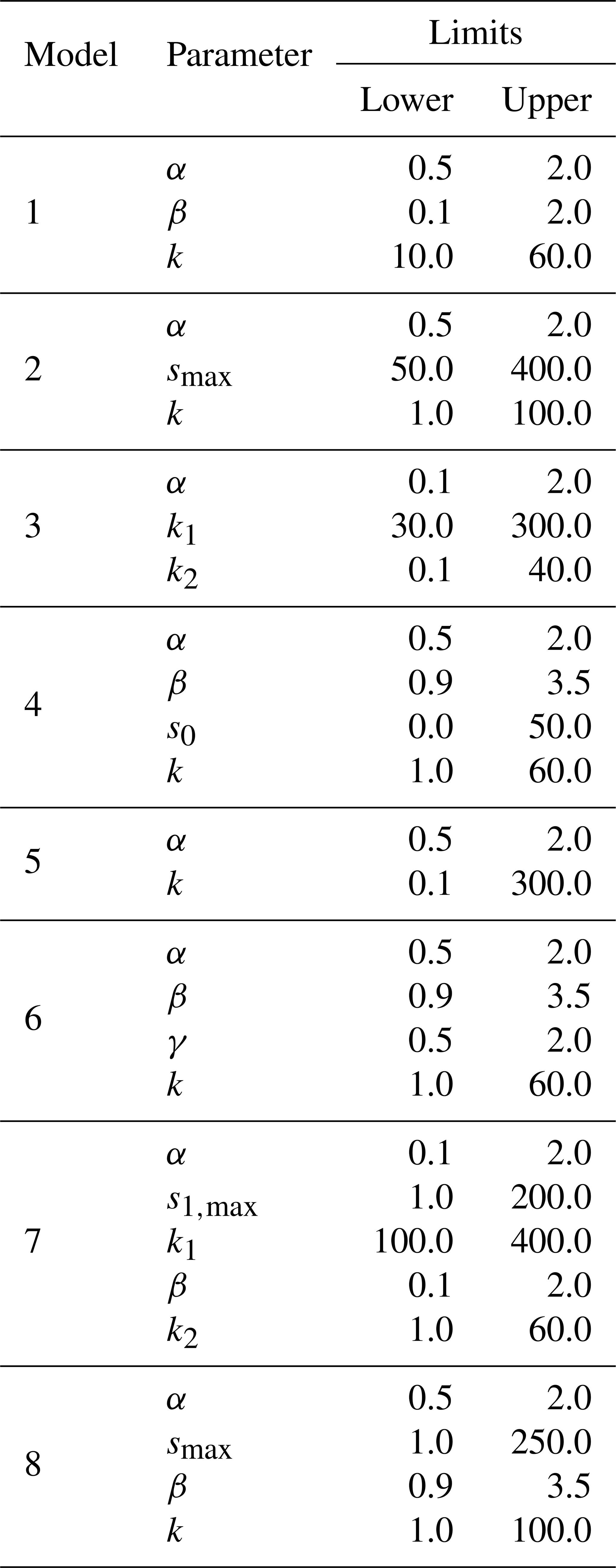
A2 CAMELS-GB
The parameter ranges for the conceptual models used in the CAMELS-GB case are listed in Table A2. The parameter ranges shown in both Tables A1 and A2 were adapted from typical ranges found in the literature for the HBV model (Beck et al., 2016, 2020). For the synthetic examples, we simplified the parameter ranges to better suit the proposed examples. The static attributes used as input to the LSTM in all models are listed in Table A3.
Table A2Ranges of the model parameters for the CAMELS-GB case study.
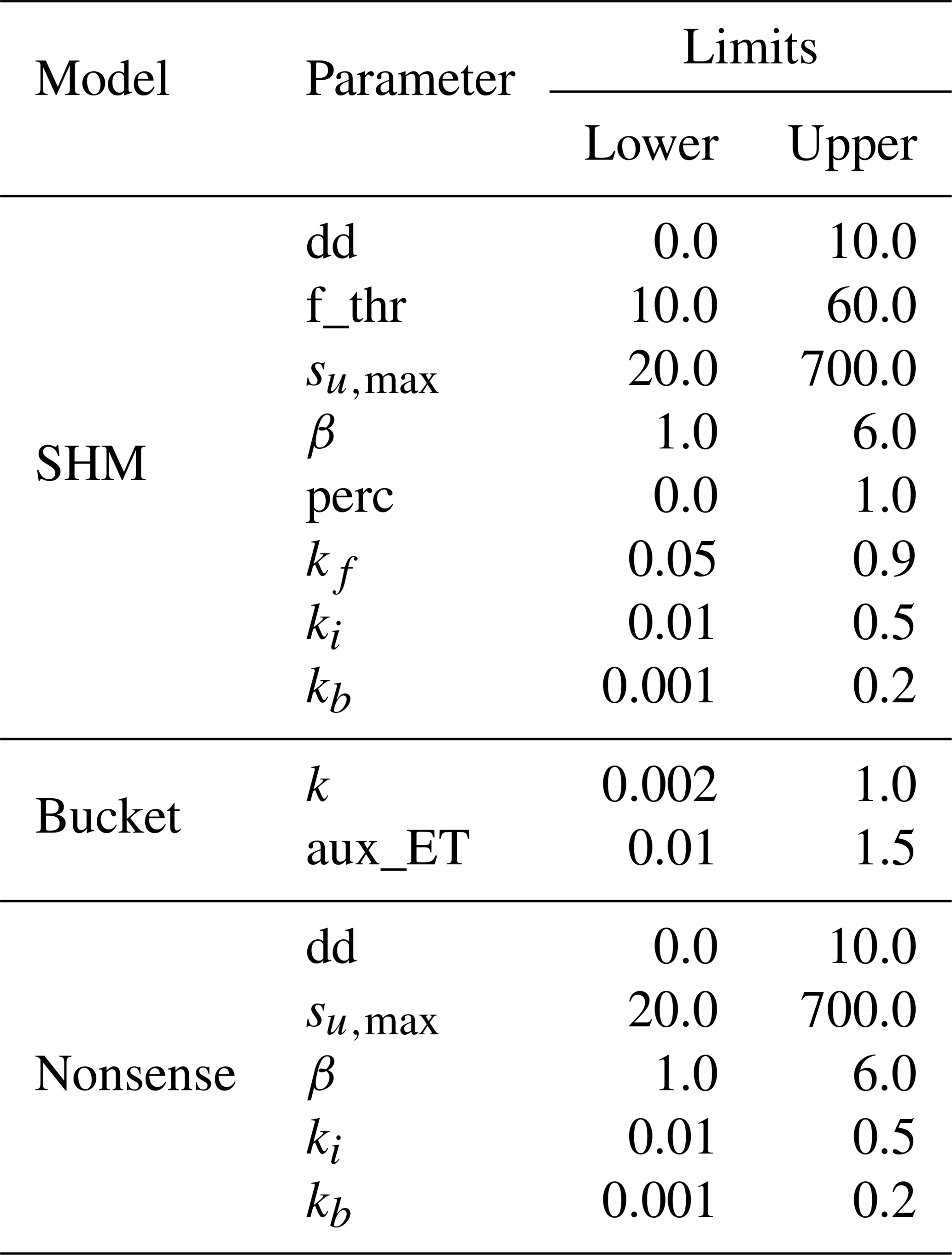
Table A3Catchment attributes from the CAMELS-GB dataset used to train all models.
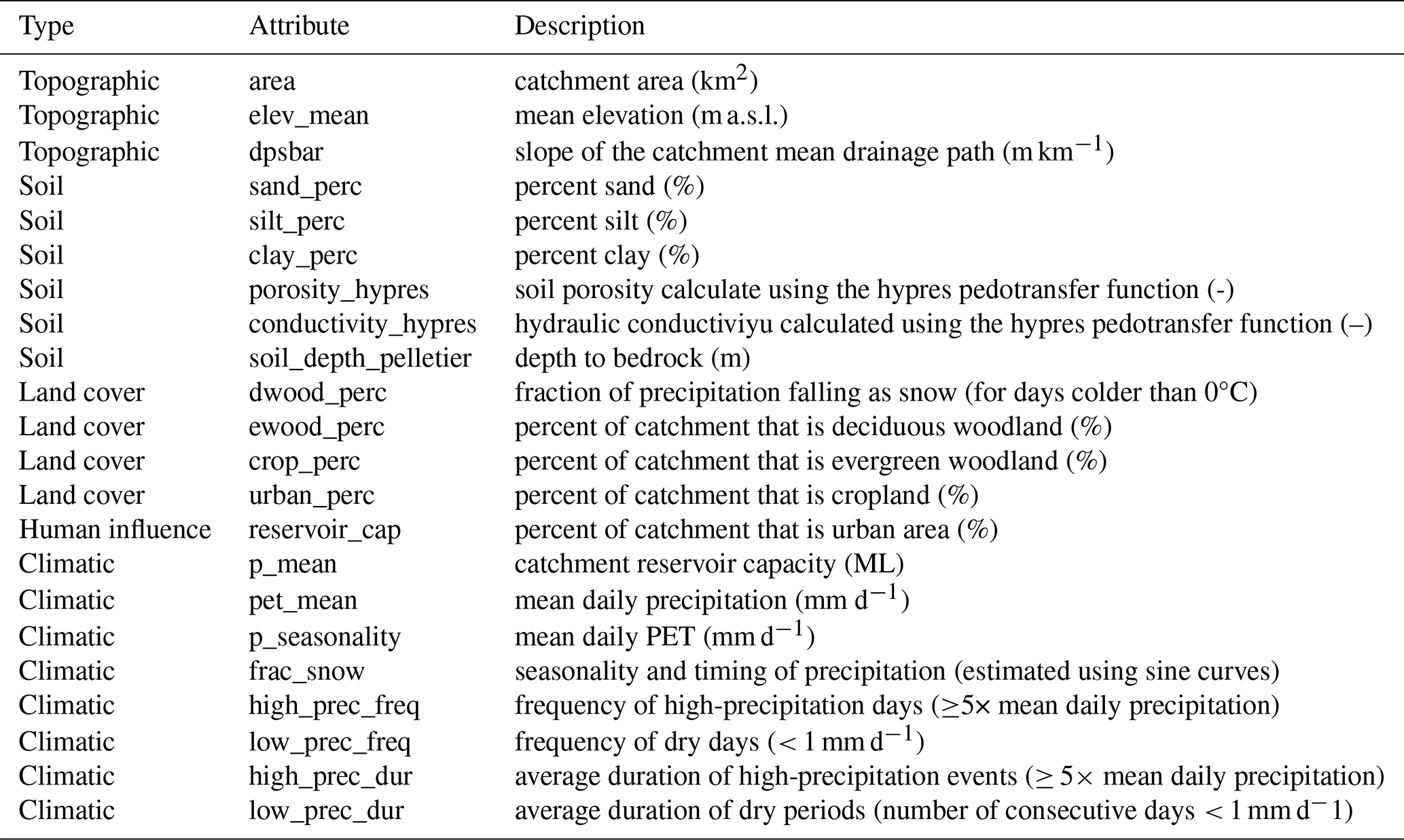
In Sect. 3 and specifically Fig. 2 we showed five key didactic cases that can be used to understand the rankings in Figs. 3 and 4. To further our understanding of the behaviors that can be quantified by measuring the entropy of the hidden states of the LSTM, we show four additional examples in Fig. B1. These additional examples also follow in the framework of multiple working hypotheses (Clark et al., 2011), and in this section we briefly describe what can be learned from them.
Model 5 represents a case in which the added knowledge is lacking the degrees of freedom that the “true” model has. Thus, the LSTM has to take over and compensate using its internal hidden states, resulting in the high measurement of entropy of the LSTM. Although this behavior is also apparent in the variations of the parameters shown in Fig. B1e, measuring entropy there can result in the wrong assumption that a conceptual model with more reservoirs in Model 3 would more closely resemble the “true” model, as shown in Fig. 3 but this is not true. The true picture is given by the entropy of the LSTMs in Fig. 4.
Models 6 to 8 all serve as cases where the conceptual model has a greater number of parameters than the “true” model, making them overparametrized but cases such as 6 and 8 resemble the “true” model very closely. Model 7 also has the “true” model embedded within, but the input relationship is distorted by the extra reservoir in s1.
Returning to the idea of how much a model closely matches the “true” model, the ranking in Fig. 4 makes intuitive sense. The “true” model is furthest to the left followed by Models 4, 6 and 8 which use the same number of reservoirs and whose input-output relationships can match that of the “true” model (all have an exponential term). This grouping is followed by Model 7 which has the ability to match the output relationship using the second exponential reservoir but the input is not directly precipitation and evapotranspiration but some dampened product coming from the first reservoir. Next we have the divider between encoding “good” and “bad” physics. All of the previous models have the “true” model (in some sense) within their structure. This additional knowledge makes the task required of the LSTM easier, thus reducing its entropy. If, instead, we encode “bad” physics, we fall in cases where the model is able to perfectly fit the observed data but not because of the additional knowledge, but because of a more complex LSTM which now, in addition to prediction, has to overwrite our incorrect prior knowledge.
Model 3 is the worst offender as the usage of a two reservoirs system with none of the reservoirs having an exponential term in their output relationship is the case most dissimilar to the “true” model. Models 2 and 5 improve upon this condition, but still lack some semblance of the “true” model in their structure making them to also fall in the “bad” physics category.
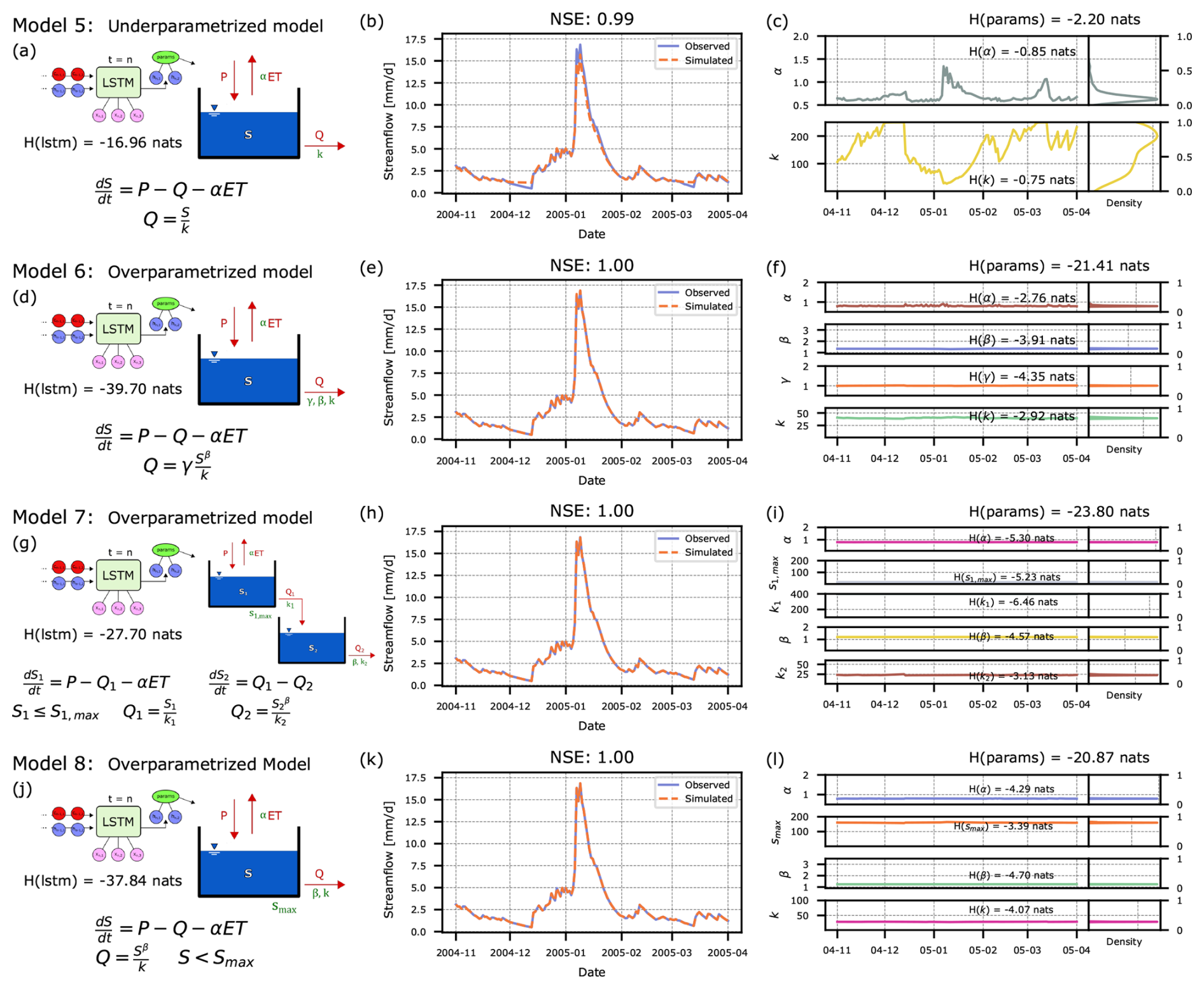
Figure B1Additional examples on evaluating hybrid hydrological models by measuring the entropy of different model components.
The results in the case study presented in Sect. 4 follow the results of the previous study of Acuña Espinoza et al. (2024). However the data and metrics reported between studies related to model variables and performance are not the same. Between studies we modified our training pipelines to adopt current standard practices (Shen et al., 2023; Kratzert et al., 2024), therefore there are differences between the metrics.
For the models with static parameters, these differences are shown in Fig. C1 and Table C1. In our previous study, the conceptual models were calibrated individually for each basin using the DREAM algorithm (Vrugt, 2016). This procedure results in better performance at predicting streamflow than in regional training as we did for this current study. The drop in performance could be the due to the identification of regional sets of parameters, as in Tsai et al. (2021), but we did not pursue this finding further.
Then for the models with dynamic parameters, the differences are shown in Fig. C2 and Table C2.
As in all cases the differences in metrics between studies are small, we accept them while acknowledging that the models analyzed in this study are different than those in Acuña Espinoza et al. (2024). Moreover, the main objective of the present study is not to set a “state-of-the-art” benchmark for a particular dataset and, accordingly, the overall message that we wish to communicate is not affected by the differences in performance between studies.
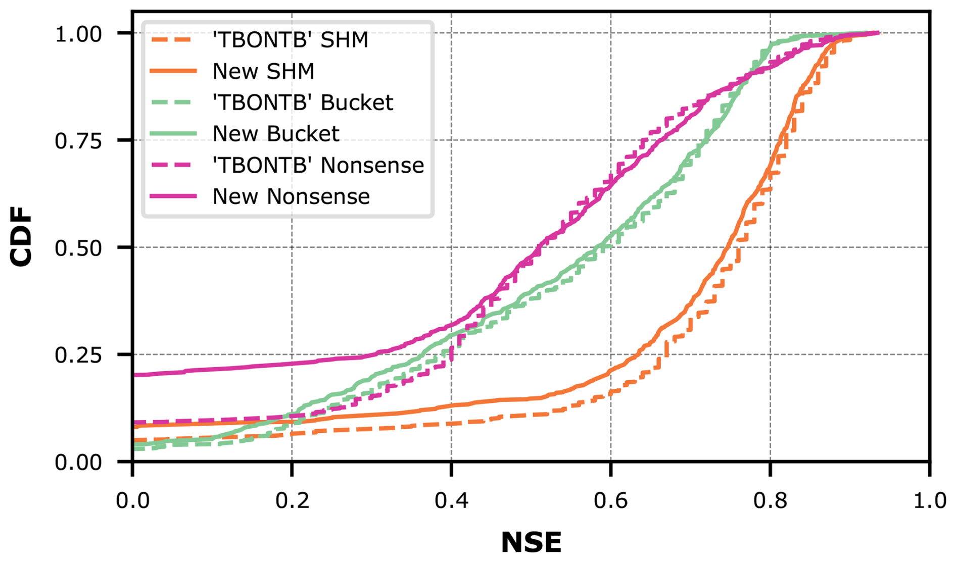
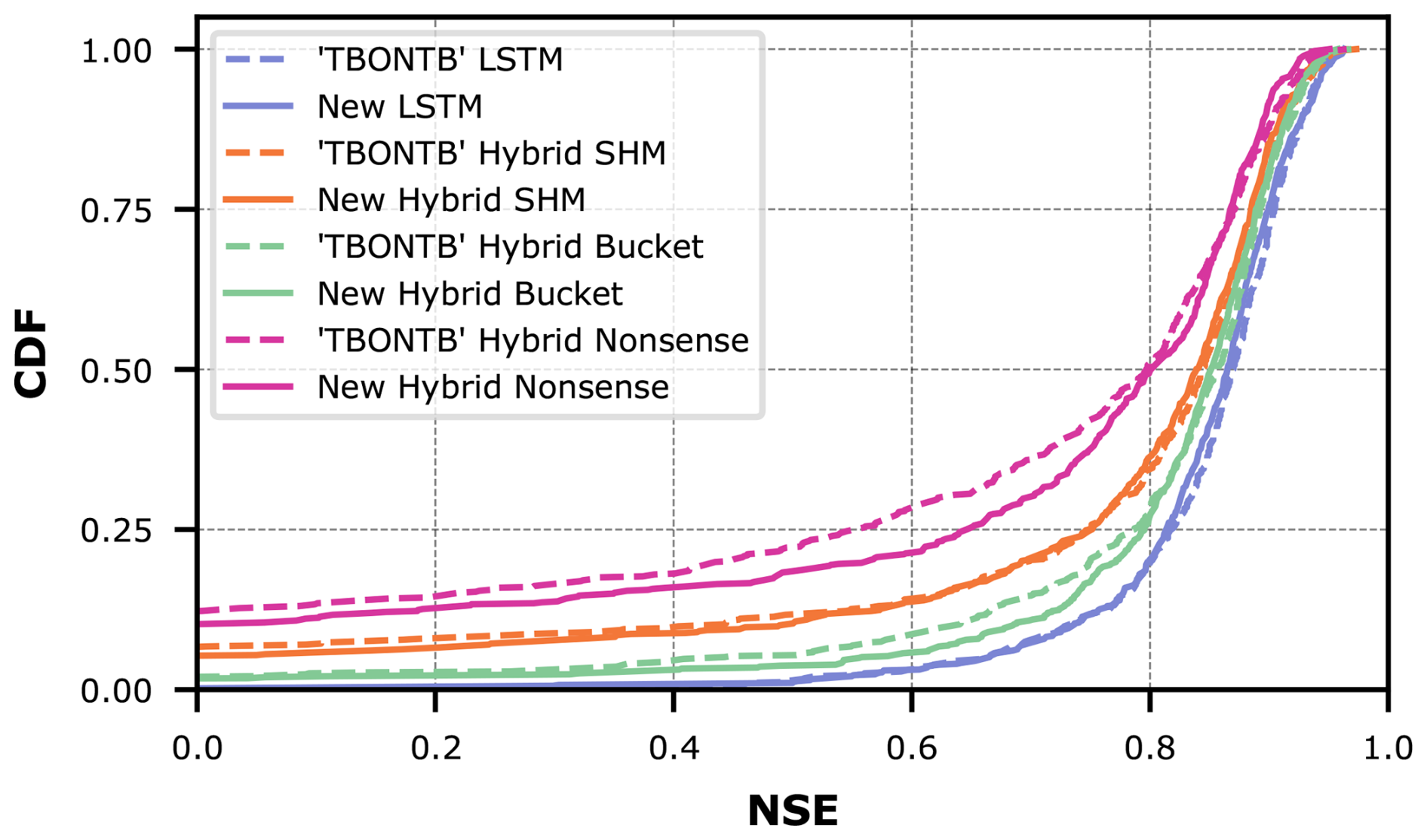
Figure C2Comparison of model performance for models with dynamic parameters between studies.
Table C1Comparison of model performance for models with static parameters quantified by area under the NSE curve (AUC) and median NSE.
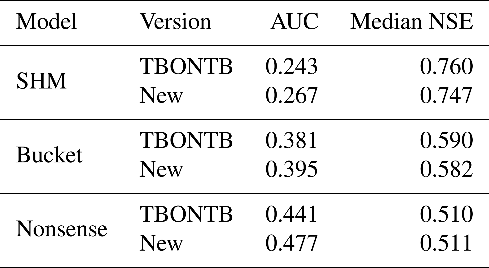
Table C2Comparison of model performance quantified by area under the NSE curve (AUC) and median NSE.
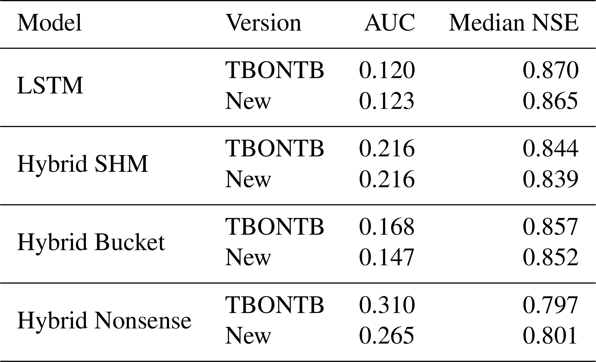
An archived version of the codebase used for this study is provided in the repository indicated in the data availability section of this paper. We also used the Hy2DL library (https://doi.org/10.5281/zenodo.17251944, Acuna et al., 2025) and the UNITE toolbox, which is available at https://github.com/manuel-alvarez-chaves/unite_toolbox (last access: 25 March 2025; https://doi.org/10.18419/DARUS-4188, Álvarez Chaves et al., 2024).
CAMELS-GB is available at https://doi.org/10.5285/8344e4f3-d2ea-44f5-8afa-86d2987543a9 (Coxon et al., 2020b). All of the code for this project, model state dictionaries, model configurations, training logs and netCDF files of the results of this study have been archived at the data repository of the University of Stuttgart (DaRUS) and can be found at this link: https://doi.org/10.18419/DARUS-4920 (Álvarez Chaves, 2025).
The original idea of the paper was developed by all authors. The codes were written by EAE and MAC. The simulations were conducted by MAC. Results were discussed by all authors. The draft was prepared by MAC and AG. Reviewing and editing was provided by all authors. Funding was acquired by AG and UE. All authors have read and agreed to the current version of the paper.
The contact author has declared that none of the authors has any competing interests.
Publisher’s note: Copernicus Publications remains neutral with regard to jurisdictional claims made in the text, published maps, institutional affiliations, or any other geographical representation in this paper. While Copernicus Publications makes every effort to include appropriate place names, the final responsibility lies with the authors. Views expressed in the text are those of the authors and do not necessarily reflect the views of the publisher.
We acknowledge funding by the Deutsche Forschungsgemeinschaft (DFG, German Research Foundation) under Germany's Excellence Strategy–EXC 2075–390740016 and project 507884992. We would also like to thank Hoshin V. Gupta for his encouragement and thoughtful discussion of the results in this paper and their relationship to model complexity. Finally, we thank Georgios Blougouras, Shijie Jiang, and one anonymous reviewer for their constructive comments, which provided insightful viewpoints on our work and helped us improve the perspective of the article.
This research has been supported by the Deutsche Forschungsgemeinschaft (grant nos. EXC 2075–390740016 and 507884992).
This open-access publication was funded by the University of Stuttgart.
This paper was edited by Fabrizio Fenicia and reviewed by Georgios Blougouras, Shijie Jiang, and one anonymous referee.
Aboelyazeed, D., Xu, C., Hoffman, F. M., Liu, J., Jones, A. W., Rackauckas, C., Lawson, K., and Shen, C.: A differentiable, physics-informed ecosystem modeling and learning framework for large-scale inverse problems: demonstration with photosynthesis simulations, Biogeosciences, 20, 2671–2692, https://doi.org/10.5194/bg-20-2671-2023, 2023. a
Acuna, E., Álvarez Chaves, M., Dolich, A., and Manoj J, A.: Hy2DL: Hybrid Hydrological modeling using Deep Learning methods, Zenodo [code], https://doi.org/10.5281/zenodo.17251944, 2025. a
Acuña Espinoza, E., Loritz, R., Álvarez Chaves, M., Bäuerle, N., and Ehret, U.: To bucket or not to bucket? Analyzing the performance and interpretability of hybrid hydrological models with dynamic parameterization, Hydrol. Earth Syst. Sci., 28, 2705–2719, https://doi.org/10.5194/hess-28-2705-2024, 2024. a, b, c, d, e, f, g, h
Addor, N. and Melsen, L. A.: Legacy, Rather Than Adequacy, Drives the Selection of Hydrological Models, Water Resources Research, 55, 378–390, https://doi.org/10.1029/2018WR022958, 2019. a
Addor, N., Newman, A. J., Mizukami, N., and Clark, M. P.: The CAMELS data set: catchment attributes and meteorology for large-sample studies, Hydrol. Earth Syst. Sci., 21, 5293–5313, https://doi.org/10.5194/hess-21-5293-2017, 2017. a, b
Álvarez Chaves, M.: Replication Data for: An entropy-based evaluation of conceptual constraints in hybrid hydrological models, V1, Data Repository of the University of Stuttgart (DaRUS) [data set] and [code], https://doi.org/10.18419/DARUS-4920, 2025. a, b
Álvarez Chaves, M., Ehret, U., and Guthke, A.: UNITE Toolbox, V1, Data Repository of the University of Stuttgart (DaRUS) [code], https://doi.org/10.18419/DARUS-4188, 2024. a
Ansel, J., Yang, E., He, H., Gimelshein, N., Jain, A., Voznesensky, M., Bao, B., Bell, P., Berard, D., Burovski, E., Chauhan, G., Chourdia, A., Constable, W., Desmaison, A., DeVito, Z., Ellison, E., Feng, W., Gong, J., Gschwind, M., Hirsh, B., Huang, S., Kalambarkar, K., Kirsch, L., Lazos, M., Lezcano, M., Liang, Y., Liang, J., Lu, Y., Luk, C. K., Maher, B., Pan, Y., Puhrsch, C., Reso, M., Saroufim, M., Siraichi, M. Y., Suk, H., Zhang, S., Suo, M., Tillet, P., Zhao, X., Wang, E., Zhou, K., Zou, R., Wang, X., Mathews, A., Wen, W., Chanan, G., Wu, P., and Chintala, S.: PyTorch 2: Faster Machine Learning Through Dynamic Python Bytecode Transformation and Graph Compilation, in: 29th ACM International Conference on Architectural Support for Programming Languages and Operating Systems, Volume 2 (ASPLOS '24), ACM, https://doi.org/10.1145/3620665.3640366, 2024. a
Azmi, E., Ehret, U., Weijs, S. V., Ruddell, B. L., and Perdigão, R. A. P.: Technical note: “Bit by bit”: a practical and general approach for evaluating model computational complexity vs. model performance, Hydrol. Earth Syst. Sci., 25, 1103–1115, https://doi.org/10.5194/hess-25-1103-2021, 2021. a
Bandai, T., Ghezzehei, T. A., Jiang, P., Kidger, P., Chen, X., and Steefel, C. I.: Learning Constitutive Relations From Soil Moisture Data via Physically Constrained Neural Networks, Water Resources Research, 60, e2024WR037318, https://doi.org/10.1029/2024WR037318, 2024. a
Beck, H. E., van Dijk, A. I. J. M., de Roo, A., Miralles, D. G., McVicar, T. R., Schellekens, J., and Bruijnzeel, L. A.: Global-scale regionalization of hydrologic model parameters, Water Resources Research, 52, 3599–3622, https://doi.org/10.1002/2015WR018247, 2016. a
Beck, H. E., Pan, M., Lin, P., Seibert, J., van Dijk, A. I. J. M., and Wood, E. F.: Global Fully Distributed Parameter Regionalization Based on Observed Streamflow From 4,229 Headwater Catchments, Journal of Geophysical Research: Atmospheres, 125, e2019JD031485, https://doi.org/10.1029/2019JD031485, 2020. a
Beirlant, J., Dudewicz, E. J., Györfi, L., and Van der Meulen, E. C.: Nonparametric Entropy Estimation: An Overview, International Journal of Mathematical and Statistical Sciences, 6, 17–39, http://jimbeck.caltech.edu/summerlectures/references/Entropy estimation.pdf (last access: 20 January 2026), 1997. a
Bergström, S. and Forsman, A.: Development of a conceptual deterministc rainfall-runoff model, Hydrology Research, 4, 147–170, https://doi.org/10.2166/nh.1973.0012, 1973. a
Beven, K.: Deep learning, hydrological processes and the uniqueness of place, Hydrological Processes, 34, 3608–3613, https://doi.org/10.1002/hyp.13805, 2020. a
Bindas, T., Tsai, W.-P., Liu, J., Rahmani, F., Feng, D., Bian, Y., Lawson, K., and Shen, C.: Improving River Routing Using a Differentiable Muskingum-Cunge Model and Physics-Informed Machine Learning, Water Resources Research, 60, e2023WR035337, https://doi.org/10.1029/2023WR035337, 2024. a
Blougouras, G., Reichstein, M., Migliavacca, M., Brenning, A., and Jiang, S.: Interpretable Machine Learning to Uncover Key Compound Drivers of Hydrological Droughts, EGU General Assembly 2024, Vienna, Austria, 14–19 Apr 2024, EGU24-9639, https://doi.org/10.5194/egusphere-egu24-9639, 2024. a
Bradbury, J., Frostig, R., Hawkins, P., Johnson, M. J., Leary, C., Maclaurin, D., Necula, G., Paszke, A., VanderPlas, J., Wanderman-Milne, S., and Zhang, Q.: JAX: composable transformations of Python+NumPy programs, GitHub [code], http://github.com/jax-ml/jax (last access: 20 January 2026), 2018. a
Camus, A.: The myth of Sisyphus and other essays, Vintage Books, New York, 1st vintage international edn., ISBN 978-0-679-73373-7, 1991. a
Chlumsky, R., Mai, J., Craig, J. R., and Tolson, B. A.: Advancement of a blended hydrologic model for robust model performance, Hydrol. Earth Syst. Sci. Discuss. [preprint], https://doi.org/10.5194/hess-2023-69, 2023. a
Clark, M. P., Slater, A. G., Rupp, D. E., Woods, R. A., Vrugt, J. A., Gupta, H. V., Wagener, T., and Hay, L. E.: Framework for Understanding Structural Errors (FUSE): A modular framework to diagnose differences between hydrological models, Water Resources Research, 44, https://doi.org/10.1029/2007WR006735, 2008. a, b, c
Clark, M. P., Kavetski, D., and Fenicia, F.: Pursuing the method of multiple working hypotheses for hydrological modeling, Water Resources Research, 47, https://doi.org/10.1029/2010WR009827, 2011. a, b
Cover, T. M. and Thomas, J. A.: Elements of Information Theory, Wiley, Hoboken, N.J, 2 edn., ISBN 978-0-471-24195-9, 2006. a
Coxon, G., Addor, N., Bloomfield, J. P., Freer, J., Fry, M., Hannaford, J., Howden, N. J. K., Lane, R., Lewis, M., Robinson, E. L., Wagener, T., and Woods, R.: CAMELS-GB: hydrometeorological time series and landscape attributes for 671 catchments in Great Britain, Earth Syst. Sci. Data, 12, 2459–2483, https://doi.org/10.5194/essd-12-2459-2020, 2020a. a
Coxon, G., Addor, N., Bloomfield, J. P., Freer, J., Fry, M., Hannaford, J., Howden, N. J. K., Lane, R., Lewis, M., Robinson, E. L., Wagener, T., and Woods, R.: Catchment attributes and hydro-meteorological timeseries for 671 catchments across Great Britain (CAMELS-GB), NERC Environmental Information Data Centre [data set], https://doi.org/10.5285/8344e4f3-d2ea-44f5-8afa-86d2987543a9, 2020b. a
Craig, J. R., Brown, G., Chlumsky, R., Jenkinson, R. W., Jost, G., Lee, K., Mai, J., Serrer, M., Sgro, N., Shafii, M., Snowdon, A. P., and Tolson, B. A.: Flexible watershed simulation with the Raven hydrological modelling framework, Environmental Modelling & Software, 129, 104728, https://doi.org/10.1016/j.envsoft.2020.104728, 2020. a
Dal Molin, M., Kavetski, D., and Fenicia, F.: SuperflexPy 1.3.0: an open-source Python framework for building, testing, and improving conceptual hydrological models, Geosci. Model Dev., 14, 7047–7072, https://doi.org/10.5194/gmd-14-7047-2021, 2021. a
De la Fuente, L. A., Ehsani, M. R., Gupta, H. V., and Condon, L. E.: Toward interpretable LSTM-based modeling of hydrological systems, Hydrol. Earth Syst. Sci., 28, 945–971, https://doi.org/10.5194/hess-28-945-2024, 2024. a
Ehret, U., van Pruijssen, R., Bortoli, M., Loritz, R., Azmi, E., and Zehe, E.: Adaptive clustering: reducing the computational costs of distributed (hydrological) modelling by exploiting time-variable similarity among model elements, Hydrol. Earth Syst. Sci., 24, 4389–4411, https://doi.org/10.5194/hess-24-4389-2020, 2020. a, b
Feng, D., Liu, J., Lawson, K., and Shen, C.: Differentiable, Learnable, Regionalized Process‐Based Models With Multiphysical Outputs can Approach State‐Of‐The‐Art Hydrologic Prediction Accuracy, Water Resources Research, 58, e2022WR032404, https://doi.org/10.1029/2022WR032404, 2022. a, b, c, d
Feng, D., Beck, H., Lawson, K., and Shen, C.: The suitability of differentiable, physics-informed machine learning hydrologic models for ungauged regions and climate change impact assessment, Hydrol. Earth Syst. Sci., 27, 2357–2373, https://doi.org/10.5194/hess-27-2357-2023, 2023. a
Feng, D., Beck, H., de Bruijn, J., Sahu, R. K., Satoh, Y., Wada, Y., Liu, J., Pan, M., Lawson, K., and Shen, C.: Deep dive into hydrologic simulations at global scale: harnessing the power of deep learning and physics-informed differentiable models (δHBV-globe1.0-hydroDL), Geosci. Model Dev., 17, 7181–7198, https://doi.org/10.5194/gmd-17-7181-2024, 2024a. a
Feng, J., Li, J., Xu, C., Wang, Z., Zhang, Z., Wu, X., Lai, C., Zeng, Z., Tong, H., and Jiang, S.: Viewing Soil Moisture Flash Drought Onset Mechanism and Their Changes Through XAI Lens: A Case Study in Eastern China, Water Resources Research, 60, e2023WR036297, https://doi.org/10.1029/2023WR036297, 2024b. a
Fenicia, F., Kavetski, D., and Savenije, H. H. G.: Elements of a flexible approach for conceptual hydrological modeling: 1. Motivation and theoretical development, Water Resources Research, 47, https://doi.org/10.1029/2010WR010174, 2011. a, b, c, d
Frame, J. M., Kratzert, F., Raney II, A., Rahman, M., Salas, F. R., and Nearing, G. S.: Post-Processing the National Water Model with Long Short-Term Memory Networks for Streamflow Predictions and Model Diagnostics, JAWRA Journal of the American Water Resources Association, 57, 885–905, https://doi.org/10.1111/1752-1688.12964, 2021. a, b
Frame, J. M., Kratzert, F., Gupta, H. V., Ullrich, P., and Nearing, G. S.: On strictly enforced mass conservation constraints for modelling the Rainfall-Runoff process, Hydrological Processes, 37, e14847, https://doi.org/10.1002/hyp.14847, 2023. a
Gajamannage, K., Jayathilake, D. I., Park, Y., and Bollt, E. M.: Recurrent neural networks for dynamical systems: Applications to ordinary differential equations, collective motion, and hydrological modeling, Chaos: An Interdisciplinary Journal of Nonlinear Science, 33, 013109, https://doi.org/10.1063/5.0088748, 2023. a
Galatolo, S., Hoyrup, M., and Rojas, C.: Effective symbolic dynamics, random points, statistical behavior, complexity and entropy, Information and Computation, 208, 23–41, https://doi.org/10.1016/j.ic.2009.05.001, 2010. a
Gauch, M., Mai, J., and Lin, J.: The proper care and feeding of CAMELS: How limited training data affects streamflow prediction, Environmental Modelling & Software, 135, 104926, https://doi.org/10.1016/j.envsoft.2020.104926, 2021. a
Gong, W., Gupta, H. V., Yang, D., Sricharan, K., and Hero III, A. O.: Estimating epistemic and aleatory uncertainties during hydrologic modeling: An information theoretic approach, Water Resources Research, 49, 2253–2273, https://doi.org/10.1002/wrcr.20161, 2013. a
Goodfellow, I., Bengio, Y., and Courville, A.: Deep Learning, Adaptive computation and machine learning, MIT Press, Cambridge, Massachusetts, ISBN 978-0-262-03561-3, http://www.deeplearningbook.org (last access: 20 January 2026), 2016. a
Gupta, H. V., Wagener, T., and Liu, Y.: Reconciling Theory with Observations: Elements of a Diagnostic Approach to Model Evaluation, Hydrological Processes, 22, 3802–3813, https://doi.org/10.1002/hyp.6989, 2008. a
Harper, M.: 10 years on from the Cumbrian and Carlisle Floods of 2005, https://environmentagency.blog.gov.uk/2015/01/08/10-years-on-from-the-cumbrian-and-carlisle-floods-of-2005 (last access: 20 January 2026), 2015. a
Hochreiter, S. and Schmidhuber, J.: Long Short-Term Memory, Neural Computation, 9, 1735–1780, https://doi.org/10.1162/neco.1997.9.8.1735, 1997. a
Horton, P., Schaefli, B., and Kauzlaric, M.: Why do we have so many different hydrological models? A review based on the case of Switzerland, WIREs Water, 9, e1574, https://doi.org/10.1002/wat2.1574, 2022. a
Hrachowitz, M. and Clark, M. P.: HESS Opinions: The complementary merits of competing modelling philosophies in hydrology, Hydrol. Earth Syst. Sci., 21, 3953–3973, https://doi.org/10.5194/hess-21-3953-2017, 2017. a
Höge, M., Scheidegger, A., Baity-Jesi, M., Albert, C., and Fenicia, F.: Improving hydrologic models for predictions and process understanding using neural ODEs, Hydrol. Earth Syst. Sci., 26, 5085–5102, https://doi.org/10.5194/hess-26-5085-2022, 2022. a
Jiang, S., Zheng, Y., and Solomatine, D.: Improving AI System Awareness of Geoscience Knowledge: Symbiotic Integration of Physical Approaches and Deep Learning, Geophysical Research Letters, 47, e2020GL088229, https://doi.org/10.1029/2020GL088229, 2020. a
Kingma, D. P. and Ba, J.: Adam: A Method for Stochastic Optimization, arXiv [preprint], https://doi.org/10.48550/arXiv.1412.6980, 2017. a
Kirchner, J. W.: Catchments as simple dynamical systems: Catchment characterization, rainfall-runoff modeling, and doing hydrology backward, Water Resources Research, 45, https://doi.org/10.1029/2008WR006912, 2009. a
Kozachenko, L. F. and Leonenko, N. N.: A statistical estimate for the entropy of a random vector, Probl. Inf. Transm., 23, 95–101, https://zbmath.org/?q=an:0633.62005 (last access: 20 January 2026), 1987. a
Kratzert, F., Klotz, D., Brenner, C., Schulz, K., and Herrnegger, M.: Rainfall–runoff modelling using Long Short-Term Memory (LSTM) networks, Hydrol. Earth Syst. Sci., 22, 6005–6022, https://doi.org/10.5194/hess-22-6005-2018, 2018. a, b
Kratzert, F., Herrnegger, M., Klotz, D., Hochreiter, S., and Klambauer, G.: NeuralHydrology – Interpreting LSTMs in Hydrology, in: Explainable AI: Interpreting, Explaining and Visualizing Deep Learning, edited by: Samek, W., Montavon, G., Vedaldi, A., Hansen, L. K., and Müller, K.-R., Springer International Publishing, Cham, 347–362, ISBN 978-3-030-28954-6, https://doi.org/10.1007/978-3-030-28954-6_19, 2019a. a
Kratzert, F., Klotz, D., Herrnegger, M., Sampson, A. K., Hochreiter, S., and Nearing, G. S.: Toward Improved Predictions in Ungauged Basins: Exploiting the Power of Machine Learning, Water Resources Research, 55, 11344–11354, https://doi.org/10.1029/2019WR026065, 2019b. a
Kratzert, F., Klotz, D., Shalev, G., Klambauer, G., Hochreiter, S., and Nearing, G.: Towards learning universal, regional, and local hydrological behaviors via machine learning applied to large-sample datasets, Hydrol. Earth Syst. Sci., 23, 5089–5110, https://doi.org/10.5194/hess-23-5089-2019, 2019c. a, b
Kratzert, F., Gauch, M., Klotz, D., and Nearing, G.: HESS Opinions: Never train a Long Short-Term Memory (LSTM) network on a single basin, Hydrol. Earth Syst. Sci., 28, 4187–4201, https://doi.org/10.5194/hess-28-4187-2024, 2024. a, b, c, d
Kuhn, T. S. and Hacking, I.: The structure of scientific revolutions, University of Chicago press, Chicago, 4th edn., ISBN 978-0-226-45811-3 978-0-226-45812-0, 2012. a
Lees, T., Buechel, M., Anderson, B., Slater, L., Reece, S., Coxon, G., and Dadson, S. J.: Benchmarking data-driven rainfall–runoff models in Great Britain: a comparison of long short-term memory (LSTM)-based models with four lumped conceptual models, Hydrol. Earth Syst. Sci., 25, 5517–5534, https://doi.org/10.5194/hess-25-5517-2021, 2021. a, b
Lees, T., Reece, S., Kratzert, F., Klotz, D., Gauch, M., De Bruijn, J., Kumar Sahu, R., Greve, P., Slater, L., and Dadson, S. J.: Hydrological concept formation inside long short-term memory (LSTM) networks, Hydrol. Earth Syst. Sci., 26, 3079–3101, https://doi.org/10.5194/hess-26-3079-2022, 2022. a
Li, B., Sun, T., Tian, F., and Ni, G.: Enhancing Process-Based Hydrological Models with Embedded Neural Networks: A Hybrid Approach, Journal of Hydrology, 625, 130107, https://doi.org/10.1016/j.jhydrol.2023.130107, 2023. a
Loritz, R., Dolich, A., Acuña Espinoza, E., Ebeling, P., Guse, B., Götte, J., Hassler, S. K., Hauffe, C., Heidbüchel, I., Kiesel, J., Mälicke, M., Müller-Thomy, H., Stölzle, M., and Tarasova, L.: CAMELS-DE: hydro-meteorological time series and attributes for 1582 catchments in Germany, Earth Syst. Sci. Data, 16, 5625–5642, https://doi.org/10.5194/essd-16-5625-2024, 2024. a, b
MacKay, D. J. C.: Information theory, inference, and learning algorithms, Cambridge University Press, Cambridge, UK, New York, ISBN 978-0-521-64298-9, 2003. a
Montavon, G., Samek, W., and Müller, K.-R.: Methods for interpreting and understanding deep neural networks, Digital Signal Processing, 73, 1–15, https://doi.org/10.1016/j.dsp.2017.10.011, 2018. a
Muñoz-Sabater, J., Dutra, E., Agustí-Panareda, A., Albergel, C., Arduini, G., Balsamo, G., Boussetta, S., Choulga, M., Harrigan, S., Hersbach, H., Martens, B., Miralles, D. G., Piles, M., Rodríguez-Fernández, N. J., Zsoter, E., Buontempo, C., and Thépaut, J.-N.: ERA5-Land: a state-of-the-art global reanalysis dataset for land applications, Earth Syst. Sci. Data, 13, 4349–4383, https://doi.org/10.5194/essd-13-4349-2021, 2021. a
Nearing, G. S., Sampson, A. K., Kratzert, F., and Frame, J.: Post-Processing a Conceptual Rainfall-Runoff Model with an LSTM, Earth ArXiv, https://eartharxiv.org/repository/view/122/ (last access: 20 January 2026), 2020. a, b
Nearing, G. S., Kratzert, F., Sampson, A. K., Pelissier, C. S., Klotz, D., Frame, J. M., Prieto, C., and Gupta, H. V.: What Role Does Hydrological Science Play in the Age of Machine Learning?, Water Resources Research, 57, e2020WR028091, https://doi.org/10.1029/2020WR028091, 2021. a
Rackauckas, C., Ma, Y., Martensen, J., Warner, C., Zubov, K., Supekar, R., Skinner, D., Ramadhan, A., and Edelman, A.: Universal Differential Equations for Scientific Machine Learning, arxiv [preprint], http://arxiv.org/abs/2001.04385, 2021. a
Rahmani, F., Appling, A., Feng, D., Lawson, K., and Shen, C.: Identifying Structural Priors in a Hybrid Differentiable Model for Stream Water Temperature Modeling, Water Resources Research, 59, e2023WR034420, https://doi.org/10.1029/2023WR034420, 2023. a, b
Reichert, P. and Mieleitner, J.: Analyzing input and structural uncertainty of nonlinear dynamic models with stochastic, time-dependent parameters, Water Resources Research, 45, https://doi.org/10.1029/2009WR007814, 2009. a
Reichert, P., Ammann, L., and Fenicia, F.: Potential and Challenges of Investigating Intrinsic Uncertainty of Hydrological Models With Stochastic, Time‐Dependent Parameters, Water Resources Research, 57, e2020WR028400, https://doi.org/10.1029/2020WR028400, 2021. a
Reichstein, M., Camps-Valls, G., Stevens, B., Jung, M., Denzler, J., Carvalhais, N., and Prabhat: Deep learning and process understanding for data-driven Earth system science, Nature, 566, 195–204, https://doi.org/10.1038/s41586-019-0912-1, 2019. a
Shen, C., Appling, A. P., Gentine, P., Bandai, T., Gupta, H., Tartakovsky, A., Baity-Jesi, M., Fenicia, F., Kifer, D., Li, L., Liu, X., Ren, W., Zheng, Y., Harman, C. J., Clark, M., Farthing, M., Feng, D., Kumar, P., Aboelyazeed, D., Rahmani, F., Song, Y., Beck, H. E., Bindas, T., Dwivedi, D., Fang, K., Höge, M., Rackauckas, C., Mohanty, B., Roy, T., Xu, C., and Lawson, K.: Differentiable modelling to unify machine learning and physical models for geosciences, Nature Reviews Earth & Environment, 4, 552–567, https://doi.org/10.1038/s43017-023-00450-9, 2023. a, b, c
Song, Y., Knoben, W. J. M., Clark, M. P., Feng, D., Lawson, K., Sawadekar, K., and Shen, C.: When ancient numerical demons meet physics-informed machine learning: adjoint-based gradients for implicit differentiable modeling, Hydrol. Earth Syst. Sci., 28, 3051–3077, https://doi.org/10.5194/hess-28-3051-2024, 2024. a
Spieler, D., Mai, J., Craig, J. R., Tolson, B. A., and Schütze, N.: Automatic Model Structure Identification for Conceptual Hydrologic Models, Water Resources Research, 56, e2019WR027009, https://doi.org/10.1029/2019WR027009, 2020. a, b
Staudinger, M., Herzog, A., Loritz, R., Houska, T., Pool, S., Spieler, D., Wagner, P. D., Mai, J., Kiesel, J., Thober, S., Guse, B., and Ehret, U.: How well do process-based and data-driven hydrological models learn from limited discharge data?, Hydrol. Earth Syst. Sci., 29, 5005–5029, https://doi.org/10.5194/hess-29-5005-2025, 2025. a
Tsai, W.-P., Feng, D., Pan, M., Beck, H., Lawson, K., Yang, Y., Liu, J., and Shen, C.: From calibration to parameter learning: Harnessing the scaling effects of big data in geoscientific modeling, Nature Communications, 12, 5988, https://doi.org/10.1038/s41467-021-26107-z, 2021. a, b
Vrugt, J. A.: Markov chain Monte Carlo simulation using the DREAM software package: Theory, concepts, and MATLAB implementation, Environmental Modelling & Software, 75, 273–316, https://doi.org/10.1016/j.envsoft.2015.08.013, 2016. a
Wang, Y.-H. and Gupta, H. V.: A Mass-Conserving-Perceptron for Machine-Learning-Based Modeling of Geoscientific Systems, Water Resources Research, 60, e2023WR036461, https://doi.org/10.1029/2023WR036461, 2024. a
Waskom, M.: seaborn: statistical data visualization, Journal of Open Source Software, 6, 3021, https://doi.org/10.21105/joss.03021, 2021. a
Weiler, M. and Beven, K.: Do we need a Community Hydrological Model?, Water Resources Research, 51, 7777–7784, https://doi.org/10.1002/2014WR016731, 2015. a
Young, P., Parkinson, S., and Lees, M.: Simplicity out of complexity in environmental modelling: Occam's razor revisited, Journal of Applied Statistics, 23, 165–210, https://doi.org/10.1080/02664769624206, 1996. a
Young, P. C. and Beven, K. J.: Data-based mechanistic modelling and the rainfall-flow non-linearity, Environmetrics, 5, 335–363, https://doi.org/10.1002/env.3170050311, 1994. a
Zhang, C., Li, H., Hu, Y., Shen, D., Xu, B., Chen, M., Chu, W., and Li, R.: A Differentiability-Based Processes and Parameters Learning Hydrologic Model for Advancing Runoff Prediction and Process Understanding, Journal of Hydrology, 661, 133594, https://doi.org/10.1016/j.jhydrol.2025.133594, 2025. a
Álvarez Chaves, M., Gupta, H. V., Ehret, U., and Guthke, A.: On the Accurate Estimation of Information-Theoretic Quantities from Multi-Dimensional Sample Data, Entropy, 26, 387, https://doi.org/10.3390/e26050387, 2024. a
- Abstract
- Introduction
- Data and methods
- Didactic examples illustrating the proposed workflow
- Case study: CAMELS-GB
- Conclusions
- Appendix A: Study setup
- Appendix B: Additional didactic examples
- Appendix C: Standardizing training pipelines
- Code availability
- Data availability
- Author contributions
- Competing interests
- Disclaimer
- Acknowledgements
- Financial support
- Review statement
- References