Improved seasonal hydrological forecasting for Great Britain

Great Britain's variable maritime climate has until relatively recently limited the utility of seasonal hydrological forecasts. The latest generations of seasonal atmospheric forecasting systems have created new opportunities to improve flow forecasting across Great Britain, such as for the UK Hydrological Outlook. Here, we combine newly-developed high-resolution rainfall forecasts derived from historical weather analogues (HWA) conditioned on large-scale circulation patterns with a monthly-resolution national-scale hydrological model to produce seasonal and monthly forecasts. This forecasting scheme is evaluated using hindcasts from 1993–2017. We show that the skill of the rainfall forecasts is comparable to that achieved at coarser resolutions by other models. However, increasing the spatial resolution has degraded some of the skill found by previous authors producing HWA forecasts at lower resolutions. The river flow forecasts perform better than rainfall, with much of the improvement attributable to the skill provided by hydrological initial conditions. Both rainfall and river flow forecasts are most skilful in winter and perform adequately in spring and autumn. We show that in responsive catchments, primarily found in the northwest, rainfall forecasts contribute most of the skill in the river flow predictions but are much less important in regions with long hydrological memory. We thus indicate where flow forecasts would benefit most from improved rainfall forecasts or from better hydrological modelling. The introduction of these high-resolution rainfall forecasts now enables hydrological forecasting at unprecedented levels of detail across Great Britain and demonstrates a forecasting approach that may be similarly beneficial elsewhere in the world.

1 Introduction

Seasonal and sub-seasonal hydrological forecasts, here defined as those spanning the next three months and one month, respectively, should complement shorter-term weather and longer-term climate forecasts in providing actionable intelligence for water resources managers and emergency responders to take early actions to prepare for and mitigate extreme events (e.g. Murphy et al., 2001; Hamlet, Huppert and Lettenmaier, 2002; White, Franks and McEvoy, 2015; Anghileri et al., 2016; Portele et al., 2021; Jackson-Blake et al., 2022). The performance of seasonal forecasts for the UK (in common with those for much of the extra-tropics) remains marginal (e.g. Johansson, 2007; Arribas et al., 2011; Kim et al., 2012; Vitart and Robertson, 2018; Quaglia et al., 2022; Nikraftar et al., 2024), but nevertheless these forecasts already underpin decisions to take low- and no-regret actions (those with minimal or only opportunity costs). These can include advertising to encourage reduced consumption when a seasonal forecast indicates a risk of water scarcity, or increasing the readiness of flood defences, relocating equipment and alerting staff when the forecasts indicate high river flows are probable. Improved forecast skill would support the use of management strategies with higher costs or longer lead times, such as altering reservoir stocks or activating regional water transfer schemes (e.g. Peñuela et al., 2020).

The UK national capability for seasonal hydrological forecasting is delivered through the UK Hydrological Outlook (https://hydoutuk.net, last access: 29 September 2026; Prudhomme et al., 2017; Boorman and Turner, 2019). It was established in 2013 following the 2010–2012 drought (Kendon, Marsh and Parry, 2013) and the subsequent extreme rainfall that caused flooding over the rest of 2012 (Prudhomme et al., 2017). Since then, the Hydrological Outlook has been issued monthly by a collaboration between the UK Centre for Ecology and Hydrology (UKCEH), the British Geological Survey (BGS), and the Met Office. Similar systems are also available in the USA (Demargne et al., 2014; Kirtman et al., 2014; Slater et al., 2019), Australia (Schepen and Wang, 2015), continental Europe (Alfieri et al., 2013), and sub-Saharan Africa (Sheffield et al., 2014). More recently, through the HydroSOS project, the World Meteorological Organisation has sponsored efforts to develop an equivalent global service, integrating the outputs of many national products (Jenkins et al., 2020).

The UK Hydrological Outlook comprises estimates of the current hydrological conditions and forecasts of river flows and groundwater levels for the following one- and three-month periods. River flow forecasts are derived from several methods, including a gridded hydrological model driven by meteorological observations and rainfall forecasts (Bell et al., 2013, 2017), traditional ensemble streamflow predictions (ESP; e.g. Day, 1985; Harrigan et al., 2018), and historical analogues (Svensson, 2014, 2016). Many of the modelled outputs are also made available on the Hydrological Outlooks Portal (https://ukho.ceh.ac.uk/, last access: 29 September 2026), an interactive web service allowing users to inspect detailed forecasts from each method.

Previously, Bell et al. (2013, 2017) have demonstrated the use of seasonal weather forecasts to drive the Grid-to-Grid/Water Balance Model (G2G/WBM), one of several hydrological forecasting schemes used to inform the Hydrological Outlook. The G2G/WBM scheme uses observed meteorology and the G2G hydrological model (Bell et al., 2009) to generate initial conditions (subsurface water stores). Rainfall forecasts are produced by the Met Office's Global Seasonal forecasting system version 5 (GloSea5), an ensemble prediction system based on a HadGEM3 climate model (Scaife et al., 2014; MacLachlan et al., 2015; Williams et al., 2018). The initial conditions and rainfall forecasts are then combined in a simple monthly-resolution water balance model to derive estimates of river flows.

A limitation in the system demonstrated by Bell et al. (2013) was the lack of spatial resolution in the weather forecasts. Although the climate model had a resolution of 50 km, only the UK-mean rainfall was provided operationally. Hydrological forecasting requires significantly finer resolution. The provided weather forecasts were therefore downscaled to the 1 km resolution of the hydrological model by multiplying the national rainfall anomaly by the 1 km standard average monthly rainfall. Although this method has been shown by Kay et al. (2023) to outperform assuming uniform rainfall across the country, it still assumes a spatially uniform rainfall anomaly and thus fails to capture the significant variations that are often present across the country. As a result, Bell et al. (2017) limited their assessment of hydrological forecast skill to regional-mean flow anomalies and operational forecasts issued in the Hydrological Outlook were similarly aggregated, reducing their utility.

More recently, Stringer et al. (2020) presented a new approach to produce high resolution seasonal rainfall forecasts, exploiting improvements in the prediction of the large-scale circulation patterns that drive UK rainfall (e.g. Scaife et al., 2014; Dunstone et al., 2016; Thornton et al., 2023). In this “Historic Weather Analogues” (HWA) method, a forecast ensemble is constructed by combining observed rainfall patterns in years with similar circulation patterns to those predicted by GloSea. This allows the rainfall forecasts to be constructed at the native 1 km resolution of the G2G/WBM hydrological models, potentially offering improved performance at these resolutions. Stringer et al. (2020) assessed the correlation of the ensemble mean of winter (December, January, February) total rainfall forecasts over northern Europe and showed that the HWA forecasts correlate better with observations than the GloSea5 forecasts from which they are derived.

In this work, we evaluate the use of HWA rainfall forecasts in the G2G/WBM hydrological forecasting scheme across the entire year. This scheme has been used operationally within the UK Hydrological Outlook since December 2023. An illustration of the forecasts over this period is provided in the Supplement. This is the first application of these HWA rainfall forecasts to gridded and national-scale seasonal hydrological forecasting in Great Britain. At catchment scales, Donegan et al. (2021) have compared the performance of traditional “historical ESP” with HWA-derived rainfall forecasts (referred to as “conditioned ESP”) to drive hydrological forecasts for selected catchments in the Republic of Ireland over the winter. They concluded that this approach outperforms “historical ESP” in almost all catchments at one- and two-month lead times. It furthermore remained skilful at three-month lead times where “historical ESP” had practically no skill. They therefore recommended that “conditioned ESP” (HWA) is made operational in Ireland. Similar work is now in progress to apply HWA forecasts to catchment models in Great Britain (Chan et al., 2026).

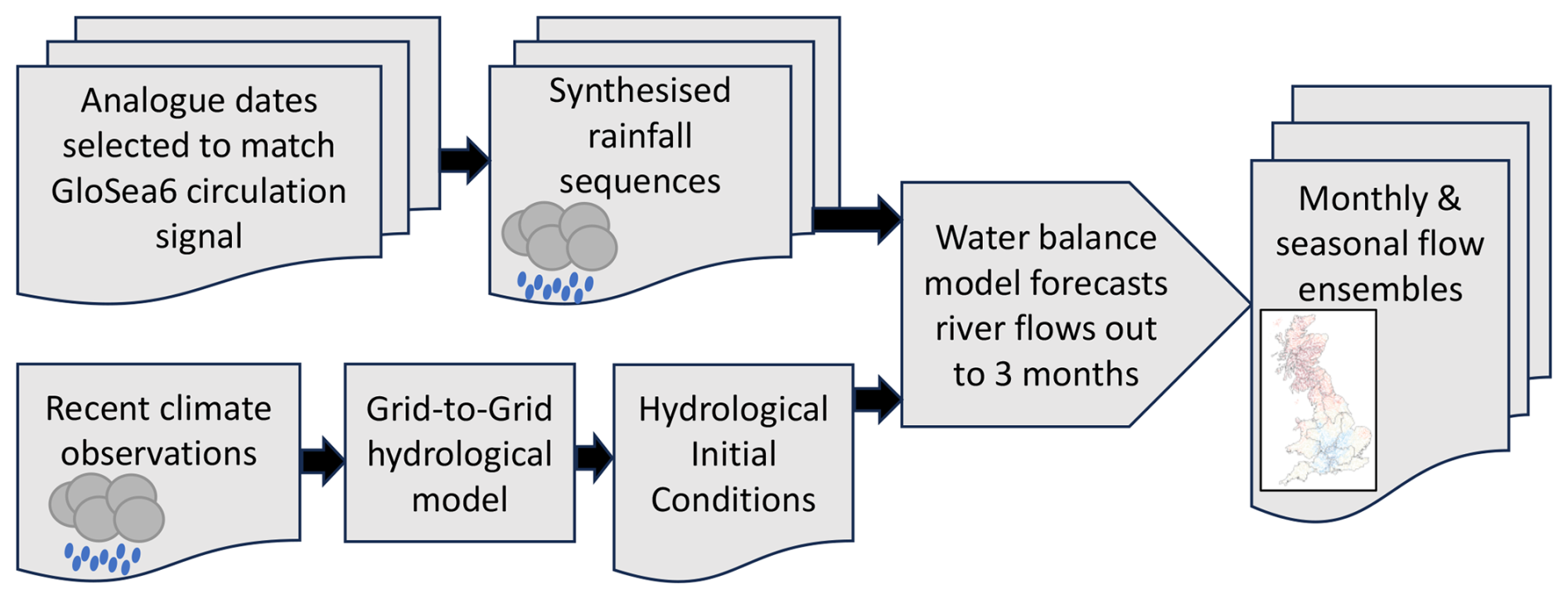
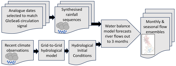
Figure 1 Schematic of the G2G/WBM hydrological forecasting scheme, here driven by rainfall forecasts derived from Historic Weather Analogues. An extended version of this figure with greater detail on the rainfall forecasting method is in the Supplement.

This paper is structured as follows. In Sect. 2 we describe our hydrological forecasting scheme and the set of hindcasts and performance scores used to assess its performance. In Sect. 3 we examine the performance of the HWA rainfall forecasts, extending the earlier assessment of Stringer et al. (2020) beyond the winter season. We then assess the performance of river flow forecasts driven by the rainfall forecasts in Sect. 4, concluding with a comparison to the earlier forecasting scheme by Bell et al. (2017). In Sect. 5 we explore the relative contributions of rainfall forecasts and hydrological initial conditions to the skill of river flow forecasts across the UK. We conclude in Sect. 6.

2 Methods

2.1 Forecasting River Flows

The G2G/WBM method for forecasting river flows comprises three stages, summarised in Fig. 1:

• 1.

  Hydrological initial conditions (HICs) are estimated using a run of the G2G hydrological model over preceding months driven by observed rainfall and actual evaporation, up to the forecast time origin.

• 2.

  Rainfall forecasts are constructed from historical rainfall data using HWA forecasts.

• 3.

  These two inputs are used to drive the Water Balance Model to forecast river flows.

Here, we describe each of these steps in greater detail. All data are generated, and models run, on the Ordnance Survey GB National Grid (EPSG:27700) at 1 km spatial resolution. We refer below to “seasonal” and “monthly” forecasts as those spanning the next three months and one month, respectively.

2.1.1 Hydrological Initial Conditions

The initial conditions for the Water Balance Model consist of simulated estimates of the subsurface water stores at 9am GMT on the first day of each month (i.e. the start of the first “water day”). Each month's initial stores are estimated using a G2G run beginning from the initial states at 9am on the first day of the previous month and incrementing in 15 min timesteps over that month. The model runs on 365 d years (and 366 d leap years), correctly handling variable month lengths and leap days.

Meteorological inputs for the G2G run are provided by the Met Office and comprise the latest 1 km resolution daily total rainfall from HadUK-Grid¹, and potential evaporation at 40 km resolution produced using the Met Office Rainfall and Evaporation Calculation System v2.0 (MORECS; Hough and Jones, 1997), the latter uniformly downscaled to the 1 km model resolution and both uniformly disaggregated from daily totals to the 15 min resolution of the model. Although simplistic, adopting this uniform temporal downscaling will be sufficient for monthly and seasonal forecasting; more sophisticated approaches are important for nearer-term forecasts. The model connects together a probability-distributed model (PDM; Moore, 2007) for rainfall-runoff generation, a modified kinematic-wave routing scheme (Bell et al., 2009) for lateral flow on the surface and in a subsurface layer with flow directions derived from the UKCEH Integrated Hydrological Digital Terrain Model (IHDTM), and a return flow path. The G2G model is described in detail by Bell et al. (2009).

Hydrological initial conditions are available from 31 December 1962, based on model runs initialised from January 1961 and allowing 2 years for the model to reach equilibrium.

2.1.2 Historic Weather Analogues rainfall forecasts

The Water Balance Model requires monthly total rainfall forecasts as an input. There are a variety of methods that could be used to generate such forecasts, which fall on a spectrum ranging from the use of raw outputs from process-based atmospheric models to the use of historical sequences with no knowledge of contemporary atmospheric conditions (above described as “historical ESP”). The HWA forecasting approach sits in the centre ground. Much like the use of raw model outputs (and unlike historical ESP), such forecasts are sensitive to contemporary atmospheric conditions. However, like traditional historical ESP (and unlike purely process-based models) they also benefit from our understanding of historical variations in weather patterns at high spatial resolutions.

The HWA approach taken in this work is an extension of that presented in Stringer et al. (2020) and Donegan et al. (2021). A detailed description of this method is given in the Supplement; here we outline the key steps. We first construct a ca. 40-member lagged ensemble of GloSea6 (Kettleborough et al., 2026) Mean Sea Level Pressure (MSLP) forecasts covering the North Atlantic and Europe from runs initialised over the preceding days. A set of synthetic MSLP observations, constructed by combining observations from three “analogue” years, are also produced. For each GloSea6 ensemble member, we then rank synthetic observations by their root mean squared difference to the member's forecast MSLP field and select the best ten to become members of our HWA forecast ensemble. The final HWA rainfall forecasts are then made from the HadUK-Grid (Met Office, 2024) observed rainfall in these analogue years, with a linear correction for the effects of climate change applied.

However, for seasonal forecasts from November–December–January to February–March–April (inclusive), we first amplify the North Atlantic Oscillation (NAO) signal in the GloSea6 MSLP ensembles. This is to correct for the “signal to noise paradox” (Scaife and Smith, 2018; Stringer et al., 2020), in which the ensemble mean variance is smaller than is consistent with its relatively high correlation with observations. The approach taken to construct the set of synthetic seasons is modified to emphasise this signal by only choosing analogue years with a similar (within 4 hPa) monthly-mean NAO index to that in the adjusted GloSea6 ensemble member (Stringer et al., 2020). These synthetic seasons are then ranked by the root mean squared difference in their residual MSLP fields, the best ten selected, and rainfall forecasts constructed in the same manner as in other seasons.

2.1.3 River flow forecasts using the Water Balance Model

Forecasts of river flows are produced by a simple water balance model originally presented by Bell et al. (2013). This model operates on a 1 km spatial resolution and 1-month temporal resolution and forecasts subsurface water stores and river flows. First, stores are estimated by assuming that at each timestep the new store is the combination of the initial store, inputs from precipitation, and outputs from evaporation and outflows. The store at the end of month m+1 is thus given by

$$\begin{array}{}\text{(1)}& S_{m+\mathrm{1}}=S_m+P_{m+\mathrm{1}}-E_{m+\mathrm{1}}-Q_{m+\mathrm{1}}\end{array}$$

where S_m is the total subsurface water store at the end of month m, and P_m+1, E_m+1, and Q_m+1 the forecasted precipitation, actual evaporation and outflow over month m+1.

For the UK Hydrological Outlook implementation of the WBM, we derive the initial store S_m from the G2G run described in Sect. 2.1.1 and the forecast precipitation as described in Sect. 2.1.2. Evaporation is estimated using the monthly mean actual evaporation as estimated from a long-baseline run of G2G (see Eq. 7 of Bell et al. 2009). Outflows are estimated as a function of water storage and subject to simplifying assumptions, as discussed by Bell et al. (2017). We note that the model estimates natural flows with anthropogenic influences currently neglected; in some catchments in Great Britain these can be significant (Rameshwaran et al., 2022).

The output of the water balance model consists of 1 km grids of a forecast estimate of the next month's store S_m+1 and runoff Q_m+1. Runoff from each upstream cell is accumulated spatially to produce the final river flow forecast estimate. For seasonal forecasting, the first month uses the G2G hydrological initial conditions described in Sect. 2.1.1, with each subsequent month adopting the forecast stores from the water balance model for the preceding month.

2.1.4 Forecast products

Forecast river flows for each 1 km grid-cell are converted into flow anomalies by dividing by the corresponding long-term mean river flow from an observation-driven baseline run of the WBM from 1965–2019 (inclusive). For seasonal forecasts, after calculating anomalies for each month separately, the three months are averaged to produce a seasonal river flow forecast anomaly.

Finally, river flows are categorised into seven classes based on the historical distribution of flow anomalies. The classes follow those used in the Environment Agency Water Situation Report for ease of comparison (Fig. 2). The threshold river flow anomaly is calculated for each cell for each month, and for seasonal forecasts for each combination of three sequential months. This classification scheme expresses the forecast as a deviation from the “normal” modelled conditions for the time of year, with “exceptionally high/low” defined as exceeding 20-year return periods. Since the classes are defined as percentiles of the modelled climatology, this approach incorporates a first-order bias correction. At gauged locations bias-corrected flow forecasts can be derived using the known distribution of observed flows over the period of record, but this is not currently done operationally.

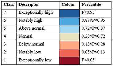
Figure 2 Classes used to categorise river flow forecasts relative to their historical distributions. Each class has a name and characteristic colour.

Table 1 Availability of hindcasts for the HWA rainfall forecasts.

^a The number of years of hindcasts available. ^b The number of rainfall ensemble members within each hindcast.

2.2 Performance Assessment methods

2.2.1 Hindcast sample

To assess the performance of both the HWA rainfall forecasts and the G2G/WBM river flow forecasts, we use a sample of hindcasts (re-forecasts of past cases). These hindcasts emulate the seasonal forecasts that would have been produced at the start of each season (DJF: Winter, MAM: Spring, JJA: Summer, SON: Autumn) and monthly forecasts that would have been produced at the start of each month. They are generated automatically within the operational GloSea6 forecasting system, which runs an array of hindcasts starting from historic initial atmospheric conditions on the 1st, 9th, 17th, and 25th of each month (MacLachlan et al., 2015; Kettleborough et al., 2026). From these we select the hindcasts that are generated at a similar lead time to the operational system (see Sect. S1 in the Supplement). For the seasonal hindcasts, these are the 17 GloSea6 hindcast members initialised on each of the 1st, 9th and 17th of the month preceding the forecast. For the monthly hindcasts, we use 7 GloSea6 members from each of the 9th and 17th. Monthly hindcasts are available from February 1993 to January 2017 and seasonal hindcasts from Spring 1993 to Winter 2016/17. This is the current international standard period used to verify seasonal forecasting systems participating in the Copernicus Climate Change Service², which includes the Met Office's GloSea6. The hindcast samples' properties are summarised in Table 1.

Using these GloSea6 hindcasts, we generate seasonal (monthly) total rainfall ensembles as described in Sect. 2.1.2. From the rainfall ensembles and the associated hydrological initial conditions (Sect. 2.1.1) we derive seasonal (monthly) mean river flow ensembles as described in Sect. 2.1.3.

2.2.2 Ground truths

The hindcasts described in Sect. 2.2.1 are to be compared with observations of the seasonal (monthly) total rainfall and mean river flows in the corresponding period. Ideally, one would compare with observations taken at the resolution of the dataset; in practice observations are not available everywhere we would wish. In this study we choose to prioritise coverage rather than restrict ourselves to only use observations taken from weather observing sites and gauging stations, and thus for both rainfall and river flows we have used “ground truth” datasets that include an element of modelling to achieve the spatial completeness we require.

For the rainfall “ground truth”, we use the 1 km HadUK-Grid dataset, which relies on interpolation to infill between observing sites, accounting for variations in topography and other local effects (Hollis et al., 2019; Met Office, 2024). For river flows, we estimate “ground truth” flows at 1 km resolution across Great Britain using the G2G model, HadUK-Grid and MORECS data as described in Sect. 2.1.1. Bell et al. (2009) verified G2G daily flows against National River Flow Archive observations and found that it achieves a median Nash–Sutcliffe efficiency (Nash and Sutcliffe, 1970) of ≈ 0.7. Subsequent works have found similar performance across the flow regime, with no systematic variations across different catchment types (Bell et al., 2012; Bell et al., 2016; Rudd et al., 2017; Formetta et al., 2018; Kay et al. 2021; Rameshwaran et al., 2022).

2.2.3 Skill scores

In this work we use three different skill scores to measure the performance of different aspects of our probabilistic forecasts: the Pearson correlation, the (Continuous) Ranked Probability Skill Score and the Relative Operating Characteristic. Our principal goal in this work is to understand the quality of the river flow forecasts, so to these we apply all three metrics. The Pearson correlation alone suffices to indicate where and when HWA forecasts contribute skill.

The Pearson correlation (PCorr) measures the linear correlation between a single forecast and the observed value of a predictand. It is thus commonly used for deterministic forecasts but is also suitable for measuring the performance of the ensemble mean of a probabilistic forecast, which is often interpreted as representing the ability of the forecast to recover the “predictable component” (the signal) of the predictand (e.g. Weisheimer et al., 2024).

The distribution of ensemble members is a measure of the modelled uncertainty in the forecast, and thus our confidence in its predictions. A performance statistic that compares a forecast distribution to an observation which penalises over- or under-confident forecasts is thus also useful. A suitable choice is the Continuous Ranked Probability Score (CRPS; e.g. Brown, 1974; Matheson and Winkler, 1976; Hersbach, 2000; Wilks, 2011), which is defined as

$$\begin{array}{}\text{(2)}& \text{CRPS}={\int }_{-\mathrm{\infty }}^{\mathrm{\infty }}\left(\text{CDF}\right(x)-H(x,o){)}^{\mathrm{2}}\mathrm{d}x\end{array}$$

where CDF(x) is the cumulative distribution function (the probability of the predictand having value less than or equal to x), H(x,o) is the Heaviside step function, i.e.

$$\begin{array}{}\text{(3)}& H(x,o)=\left\{\begin{array}{ll}\mathrm{0}& x<o\\ \mathrm{1}& x\ge o\end{array}\right.\end{array}$$

where o is the observed value of the predictand. The CRPS can thus be viewed as analogous to the squared error, comparing the cumulative distribution functions of the forecast and the observation. In practice we do not have the probability distribution function but only an ensemble drawn from that distribution. The finite size of the ensemble can bias the CRPS, so we use the “fair” CRPS, which corrects the score towards that which would be obtained from an infinite ensemble (Ferro, 2014).

In the limit of a deterministic system, a perfect forecast (a delta function at the correct value) will have a CRPS of zero. However, when a system has intrinsic uncertainty, the best forecast probability distribution will match that intrinsic uncertainty, and thus the optimal CRPS will be greater than zero. Since the intrinsic uncertainty is unknown, we instead compare the CRPS of one forecasting system to another to determine the skill. We thus calculate the Continuous Ranked Probability Skill Score (CRPSS; e.g. Wilks, 2011), defined as

$$\begin{array}{}\text{(4)}& \text{CRPSS}=\mathrm{1}-{\displaystyle \frac{〈{\text{CRPS}}_{\text{forecast}}〉}{〈{\text{CRPS}}_{\text{reference}}〉}}\end{array}$$

where angled brackets denote an average over all hindcasts and subscripts indicate the examined forecasting scheme and the reference forecasting scheme. We adopt the climatological distribution of river flows as our reference forecasting scheme. This is a 55-member ensemble consisting of the WBM estimates of river flows obtained using the observed 1 km HadUK-Grid rainfall and MORECS PE over the equivalent month or season of the years 1965–2020. The CRPSS can therefore be thought of as indicating the value added by atmospheric and hydrological modelling over assuming river flows will follow their historical patterns.

It should be noted that the CRPSS is not a direct measure of the performance of the forecasts issued to the Hydrological Outlook. This is because we categorise flows into the 7 classes given in Fig. 2. The equivalent statistics are then the Ranked Probability Score (RPS; Epstein, 1969; Murphy, 1971) and Ranked Probability Skill Score (RPSS; Wilks, 2011), which is also corrected for ensemble size (e.g. Buizza and Palmer, 1998; Müller et al., 2005; Weigel et al., 2007). Using the 7-class HOUK classification scheme shifts the domain over which the predictand is calculated from river flows (m³ s⁻¹) to quantiles of the historic distribution of river flows, which are then categorised into unequally-sized classes (varying between 5 % of the distribution at the extremes to 44 % for the central class). We thus calculate both the CRPSS (performance at predicting river flows) and the RPSS (performance at predicting the observed class).

Finally, we choose a performance statistic that assesses the ability of the forecasting system to predict extreme events, the Relative Operating Characteristic (ROC; e.g. Swets, 1973; Mason, 1982; Mason and Graham, 1999). The ROC assessment consists of assuming that the forecasting system triggers an alert whenever the forecast probability of some event exceeds a pre-defined threshold. The proportion of observed events for which an alert was triggered (the “hit rate”) and the proportion of observed non-events for which an alert was triggered (the “false alarm rate”) can then be placed onto a graph. By varying the threshold at which an alert is triggered, a curve is constructed to indicate the performance of the alert system at these thresholds. Different forecasting schemes can then be compared by integrating the area under this curve (AUC), which will vary from 0 to 1. A forecasting scheme in which an alert is triggered entirely randomly, but with the probability that the event occurs in the sample, will have an AUC=0.5. For convenience, however, we map the skilful domain of the score to match our other performance scores, such that

$$\begin{array}{}\text{(5)}& S_{\text{ROC}}=\mathrm{2}\text{AUC}-\mathrm{1}\end{array}$$

where S_ROC=1 indicates a perfect forecast (detects all events with no false positives at all probability thresholds) and S_ROC>0 indicates the forecasting scheme is skilful over the random forecast described above.

In this work we use S_ROC to evaluate the success in predicting river flow events. Specifically, we define “high” flow events as those falling in the “above normal” classification or above (classes 5, 6 and 7), and “low” events as those falling in the “below normal” classification or below (classes 1, 2 and 3), as defined in Fig. 2. This is a very conservative definition of “events” and will include values close to the 28th or 72nd percentiles which are less likely to have significant impacts. However, it is adopted due to the small number of hindcasts available. If only very extreme categories were considered, the expected number of events in the hindcast would be negligible, and the S_ROC would have a large uncertainty.

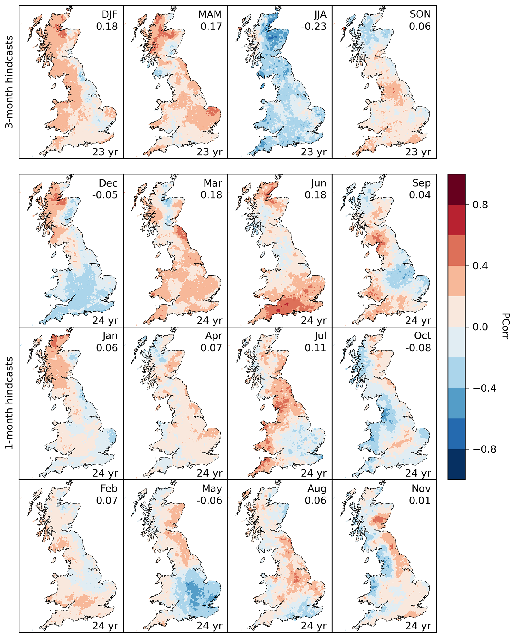
Figure 3 Pearson correlation between HWA forecast ensemble mean and observed total rainfall for 3-month (top row) and 1-month (bottom three rows) hindcasts. A positive correlation is indicated in red while a negative correlation is in blue. In each panel the number in the top-right corner is the spatial mean while the number of hindcasts used to calculate the correlation is in the bottom-right corner.

3 Performance Assessment – Rainfall Forecasts

3.1 Results

Figure 3 shows spatial maps of the Pearson correlation between the ensemble means of seasonal- (monthly-) total rainfall hindcasts and HadUK-Grid observations at 1 km resolution across Great Britain. The spatially-averaged correlation is shown in the top right of each panel as a simple indication of the relative performance in different seasons (months). However, it is the spatial variations that we consider to be of greatest importance, since these will determine over which river catchments the rainfall forecasts can offer skill. Moreover, as we will examine in Sect. 5, rivers vary in their sensitivity to recent rainfall, and thus the performance of the rainfall forecasts over regions of high sensitivity matters more than over regions of low sensitivity.

The clearest patterns in skill are apparent in the seasonal forecasts, where better performance is seen in winter (spatially averaged PCorr = 0.18, 49 % of pixels with PCorr > 0.2) and spring (0.17; 43 %) than in summer (−0.23; 0 %) or autumn (0.06; 15 %). In winter, there is a spatial pattern of higher correlations along the west coast and in northern Scotland compared to other parts of the country, while in spring the skill is less spatially coherent, with higher skill persisting in northern Scotland, but now also being seen in parts of northern England and in East Anglia. However, in only a few areas can these correlations be determined to be statistically significant (PCorr > 0.33 at 95 % confidence; Fisher and Yates, 1963). Correlations in monthly forecast skill (Fig. 3) are much more spatially and temporally variable than for seasonal forecasts, and do not systematically follow the same patterns.

3.2 Discussion

Forecasting seasonal precipitation in the extra-tropics remains extremely challenging, particularly at the high spatial resolutions demanded by hydrological forecasts. Recent studies have shown that the GloSea model used in this work is currently among the best performing models at predicting European seasonal precipitation (e.g. Quaglia et al., 2022; Nikraftar et al., 2024). However, even for the best models, correlations over the UK remain weak (typically PCorr ≈ 0.3; Baker et al., 2017, Quaglia et al., 2022). Other models which perform well in the tropics, such as the European Centre for Medium Range Weather Forecasting's SEAS5 model, show little correlation over almost all of the UK in winter and summer (PCorr < 0.2; Johnson et al., 2019). Adopting the HWA approach in winter achieves PCorr ≈ 0.4, a small improvement on the raw skill from GloSea (Stringer et al., 2020). However, all the quoted results are at much coarser resolutions (0.5–1° ≈ 25–50 km) than is required by hydrological models. At higher resolutions some of the skill will be lost as less noise is averaged out. This is demonstrated by comparing the top-left panel of our Fig. 3 with the corresponding Fig. 9 of Stringer et al. (2020), which show exactly the same hindcasts at 1 km (spatially-averaged PCorr = 0.18) and at 25 km (≈ 0.4) resolution. Reaching comparable skill at high resolutions will be necessary to fully exploit operational seasonal forecasts. Although beyond the scope of this work, additional post-processing is often used to improve seasonal rainfall forecasts elsewhere in the world and may prove useful here also (e.g. Kharin et al., 2017; Zhao et al., 2017; Shepen et al. 2018; Wang et al., 2019).

The correlations we present in Fig. 3 indicate that the performance of our HWA rainfall forecasts varies spatially as well as temporally. The best performance is visible in the winter and spring maps, where the spatial patterns correspond to the influence of the NAO upon UK rainfall. The strongest NAO influence is in December and January in northern and western parts, before it declines in later months (West et al., 2021). The widespread negative correlations in summer indicate that in this season the HWA forecasts are misleading. This results from the inability of GloSea to accurately predict summer MSLP (Lockwood et al. 2023) which, consistent with most seasonal prediction systems, struggles to capture summertime teleconnections (Knight and Scaife, 2024). However, in summer the influence of the NAO on UK rainfall becomes strong again (although with opposite sign to the winter; West et al., 2021), suggesting that the HWA method might remain appropriate if only it were conditioned on more skilful predictions.

The low spatially-averaged skill of these forecasts suggest that overall the 1 km HWA forecasts presented here offer only small improvements over climatology (which would have PCorr = 0). This explains the results of Chan et al. (2026), who found that while HWA forecasts often drove slightly more skilful catchment predictions than ESP, the latter remained difficult to beat. However, in spite of the low spatially-averaged skill, some parts of the country show substantially better performance than others, such as the north and west of Great Britain. As these are the regions where rivers are most sensitive to recent rainfall (Svensson et al., 2015), hydrological forecasts will derive more value from rainfall forecasting skill here than in less sensitive regions.

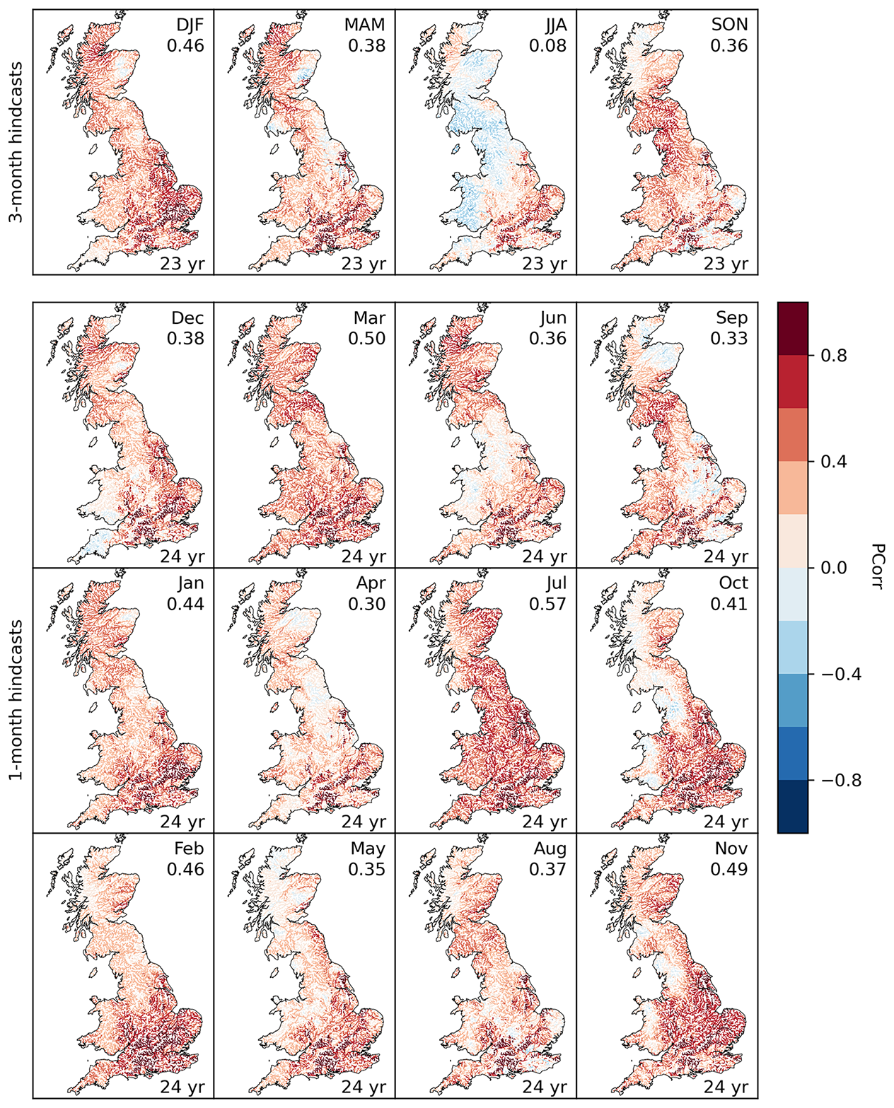
Figure 4 Pearson correlation between G2G/WBM forecast ensemble mean and “ground truth” river flows for 3-month (top row) and 1-month (bottom three rows) hindcasts. A positive correlation is indicated in red while a negative correlation is in blue. In each panel the number in the top-right corner is the spatial mean while the number of hindcasts used to calculate the correlation is in the bottom-right corner.

4 Performance Assessment – River Flow Forecasts

4.1 Results

Figure 4 shows the Pearson correlation between hindcast ensemble means and “ground truth” (simulated) river flows, both expressed in m³ s⁻¹. When flows are expressed as percentiles of the climatological distribution (as is done operationally) the correlations follow very similar spatial patterns. Here, and in the other figures in this section, we only show pixels with non-negligible annual mean runoff (> 0.05 m³ s⁻¹) which excludes highly-volatile upper reaches. Seasonal forecasting performance remains best in winter (spatially-averaged PCorr = 0.48; 90 % of river pixels with PCorr > 0.2), has similar skill in both spring (0.38; 80 %) and autumn (0.36; 75 %), but shows a substantial drop in summer (0.08; 31 %) consistent with our earlier findings for rainfall (Sect. 3). Even in summer, the strongest correlations (≈ 0.4–0.7) are found across the chalk aquifers in South-East England. Monthly forecasts show spatial patterns that are similar to the seasonal forecasts, but there is significant variability in their spatially-averaged correlations over the year.

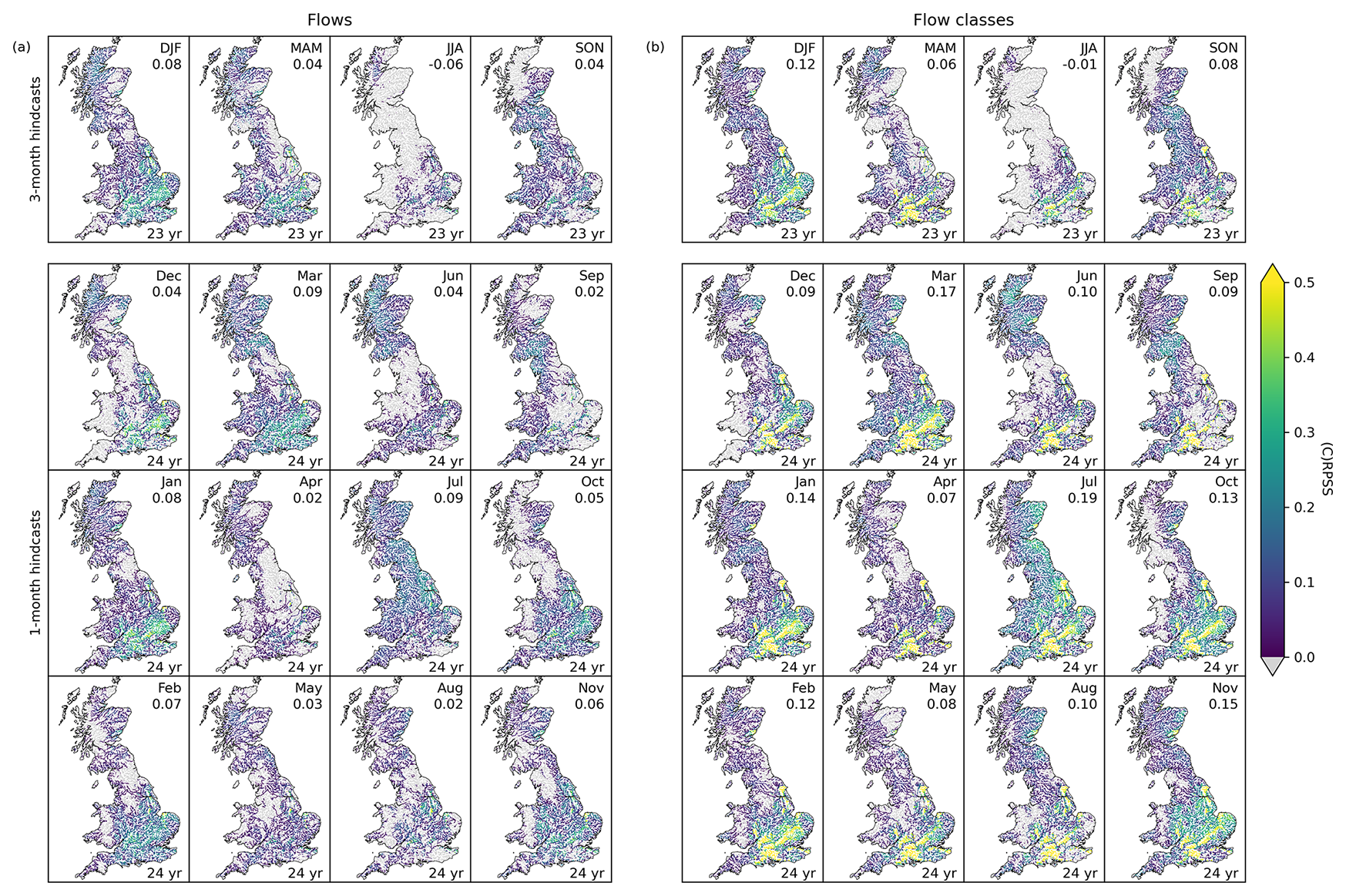
Figure 5 The skill of the G2G/WBM river flow forecasting scheme over assuming the climatological distribution. Left: CRPSS for predicting volumetric river flows (m³ s⁻¹). Right: RPSS for predicting classified flows (Fig. 2). Scores greater than 0 (coloured) indicate the G2G/WBM scheme outperforms the climatological distribution, while those less than zero (grey) indicate the converse. The spatial mean is shown in the top-right of each panel, with the number of hindcasts in the bottom-right.

Figure 5a shows the CRPSS for the G2G/WBM river flow forecasting scheme, while Fig. 5b shows the RPSS after flows are classified according to the scheme in Fig. 2. In addition to the spatial and seasonal variability observed for the ensemble means, the skill indicated for the classified forecasts systematically improves upon that for the actual river flows, with the most notable improvements across the chalk aquifers. This improvement is expected, as our classification scheme has the effect of both bias-correcting and binning forecasts. In the chalk, the uncertainty in the forecasts can often be comparable to, or smaller than, the classes such that the forecast consistently selects the observed class with high confidence.

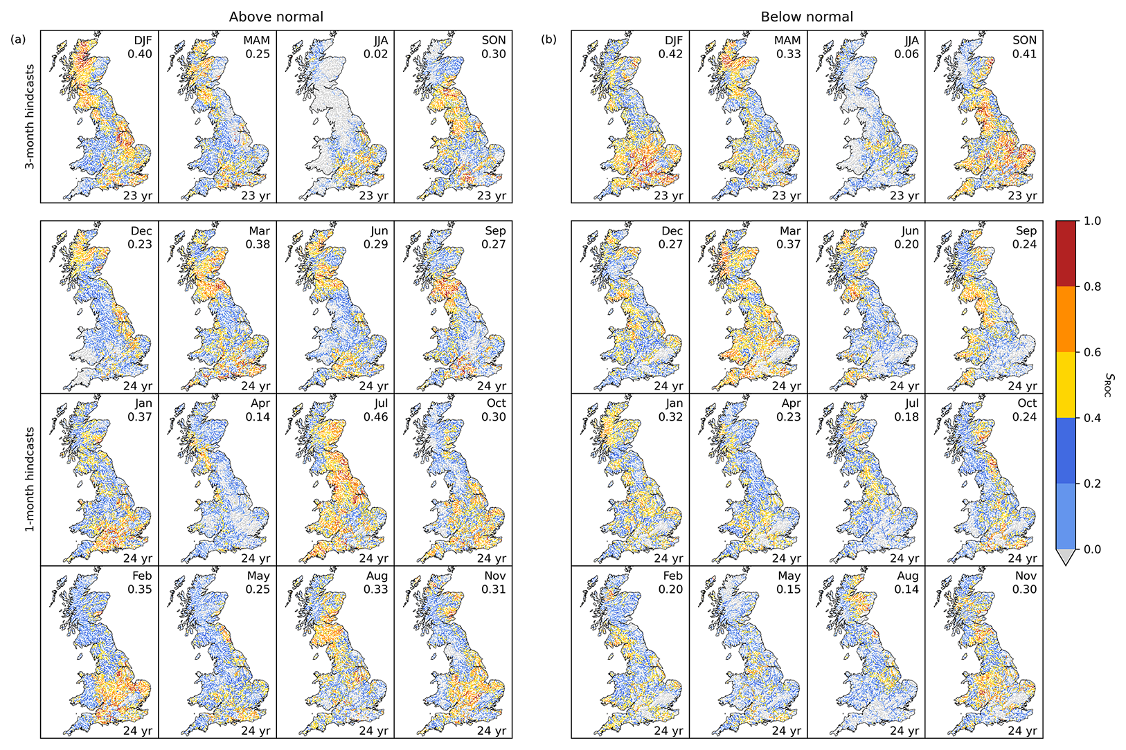
Figure 6 S_ROC for the G2G/WBM river flow forecasting scheme. The left array of panels (a) shows the performance of the model at forecasting above normal flows (> 72nd percentile) and the right array (b) shows the performance for below normal flows (< 28th percentile). Colours indicate the rescaled area under the ROC curve, with scores below 0 (grey) being inferior to a purely random process. Spatially-averaged values are shown in the top-right corner of each panel and the number of hindcasts used to calculate S_ROC is shown in the bottom-right.

Figure 6 shows the S_ROC for the performance of the G2G/WBM river flow forecasting scheme at detecting above and below normal flows. At seasonal timescales, both above- and below- normal flows are best forecast in Winter and Autumn, while at monthly timescales below-normal flows are particularly well-forecast for March, and above-normal for July. We note that although one might naïvely expect that it is easier to detect a “wet” summer or a “dry” winter, our events are defined relative to the climatological distribution of flows for the forecast period. We are thus showing the performance of the forecasting scheme at predicting a wetter-than-normal (or drier-than-normal) month/season, and the plots in Fig. 6 can be compared to one another fairly.

4.2 Discussion

Overall, the river flow forecasts perform better than the rainfall forecasts on which they were based. This is because flows in many catchments have long hydrological memory, meaning that they are less sensitive to recent rainfall. The effects of this memory are captured in our hydrological initial conditions, which contribute a significant proportion of the forecast skill for many rivers (Bell et al., 2017). A particularly clear example of this is in the southern chalk where the deep aquifer is the dominant influence on river flows. By contrast, hydrological forecasts perform less well in northern England, a region where hydrological memory is short, and where rainfall forecasts do not provide sufficient skill to underpin reliable flow forecasts.

The seasonal variations in the spatially averaged skill scores (top-right of each panel of Figs. 4–6) are consistent with the patterns for the rainfall forecasts in Fig. 3, with better relative performance in the same seasons. The skill maps show high spatial variability arising from both varying meteorological forecast skill and the differing responses of different catchments to rainfall across Great Britain. Such spatial and temporal variations in skill underline the importance of understanding where, when and how far ahead a forecasting scheme is skilful when interpreting results.

We also find that the forecast skill is not uniform across the flow regime. Figure 6 demonstrates that the forecasting scheme does not always have the same ability to detect high flows as it does low (and vice versa). An example of this can be seen by comparing the plots for July, where the scheme has significantly higher skill at detecting above-normal flows (spatially-averaged S_ROC = 0.46) than below (0.18). High and low flows arise from non-linear interactions between hydrological storage and rainfall. These non-linear interactions mean that any forecasting system is likely to exhibit such variations in performance over the flow regime.

4.3 Comparison with previous GloSea5-derived seasonal forecasts

Bell et al. (2017) assessed the skill of the previous version of the G2G/WBM hydrological forecasting scheme, which differed from that presented here in that it was driven by spatially-uniform Glosea5 rainfall forecasts. This version was used in the Hydrological Outlook prior to December 2023. Bell et al. (2017) evaluated the Pearson correlation and the S_ROC score for regional-mean river flow forecasts, which we can compare to our results (shown in Figs. 4 and 6). However, they only had a limited selection of 13 years of monthly (March, June, September, December) and seasonal (spring, summer, autumn, winter) hindcasts. Bell et al. (2017) combined Autumn-Winter and Spring-Summer hindcasts to obtain a sufficiently large sample to determine the correlation coefficient. This obscures some of the systematic variations with season found in our work.

In Autumn-Winter, Bell et al. (2017) found good correlations (PCorr ≈ 0.4–0.7) in almost all regions for both monthly and seasonal forecasts, with similar spatial patterns to ours. Our Fig. 4 shows that the winter performance is better than autumn, but the correlations remain strong over almost the entire country in both seasons. Their work also noted poor (PCorr ≈ 0.0–0.3) Spring/Summer performance across much of the country. Since Bell et al. (2017)'s forecasts were also based on rainfall outputs from GloSea, it is probable the same lack of summer meteorological skill is present (our Fig. 3 and Lockwood et al., 2023).

Table 2 GB-mean S_ROC averaged between above- and below-normal flows for the previous GloSea5-derived forecasts (Bell et al., 2017) and in this work.

Bell et al. (2017) also performed an S_ROC analysis based on the same classifications of above normal and below normal flows as in this work. Their results were aggregated spatially and temporally, and only the average S_ROC score for above- and below-normal flows presented and so their results are not directly comparable to ours. Nevertheless, we can make an approximate comparison between the GB-mean S_ROC skill scores of our Fig. 6 and those given by Bell et al. (2017); these scores are shown in Table 2. Our 1-month GB-mean S_ROC for December is now positive, compared to Bell et al. (2017)'s negative score (indicating there is now some skill). The Spring GB-mean skill score has more than doubled. These examples suggest that the introduction of HWA forecasts offers some improvement over the previous method, particularly in Winter and Spring. In these seasons, the correlations between large-scale circulation patterns and UK rainfall are strongest (Stringer et al. 2020, West et al., 2021) so the HWA forecasts (and particularly the amplification of the NAO signal) are expected to offer the greatest improvement at this time of year.

5 Sources of forecast skill

The varied hydrogeology of Great Britain drives spatially-varying sensitivity to recent rainfall and hydrological memory. Skilful river flow forecasts thus require rainfall forecasts that perform well in the regions where the rainfall is most influential. Fortuitously, the north and west of Great Britain is where both the highest sensitivity to rainfall and best performing forecasts are found (Svensson et al., 2015). Here, we are now able to explore this phenomenon for ungauged catchments across Great Britain. To do so, we have run the WBM hindcasts using three different combinations of inputs:

• a.

  HWA rainfall forecasts with climatological-mean Hydrological Initial Conditions (HICs). This combination isolates the contribution of the rainfall forecasts to the river flow forecast skill.

• b.

  All historical rainfall sequences (1965–2020) with G2G-derived HICs, equivalent to historical ESP, quantifying the contribution of the hydrological initial conditions (existing surface and subsurface water stores at the start of the forecast) to the river flow forecast skill.

• c.

  HWA rainfall forecasts with G2G-derived HICs, the forecasting scheme presented in the preceding sections which combines both rainfall and HIC forecast skill.

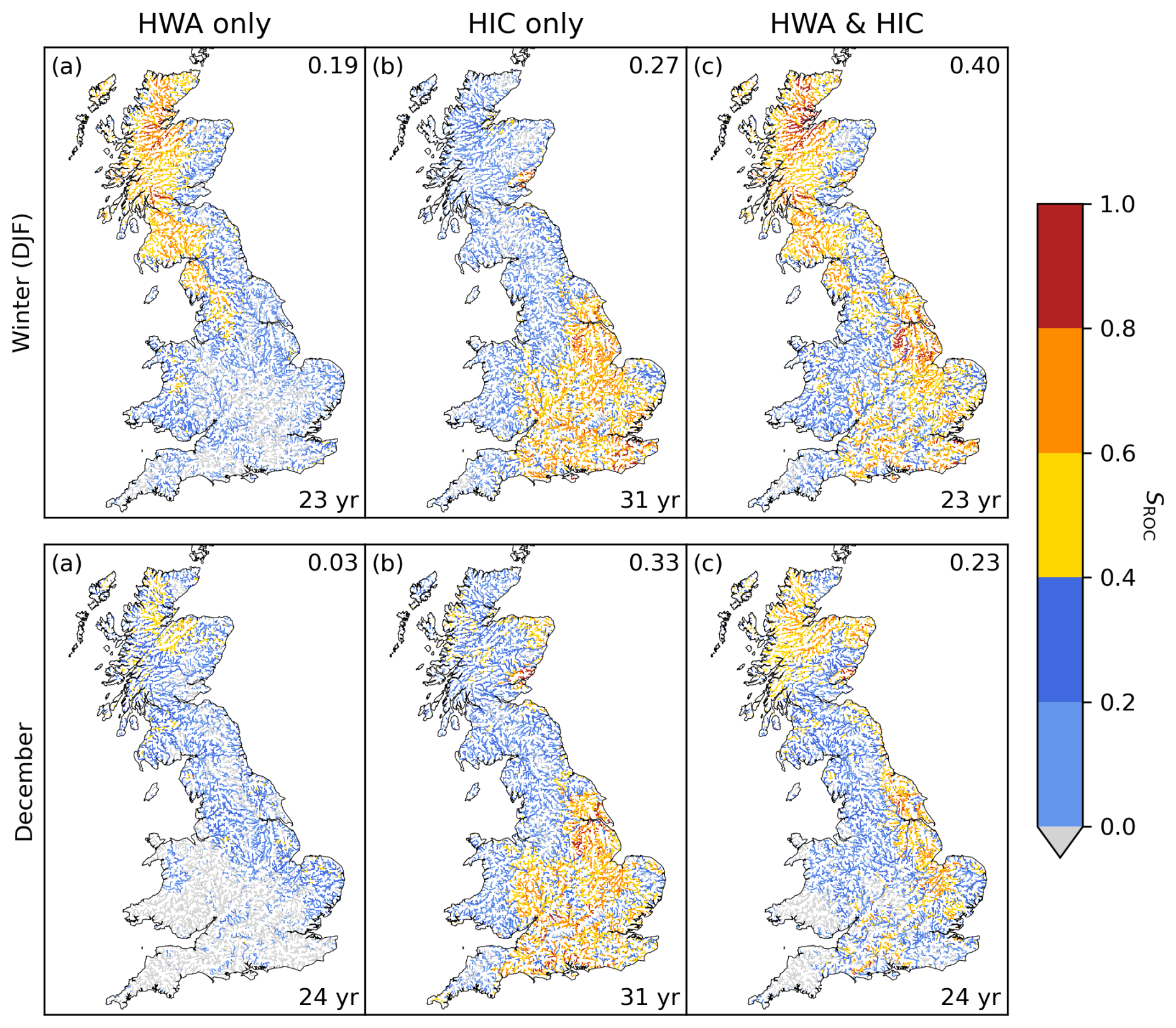
Figure 7 S_ROC for above normal river flows in Winter (top) and December (bottom) using different combinations of inputs to the WBM to highlight the contributions to forecast skill from (a): HWA rainfall forecasts (b): G2G HICs, and (c): the combination of both. Scores greater than 0 (coloured) indicate the forecasting scheme outperforms guesswork, while scores less than zero (grey) indicate the converse. The spatial means are shown in the top-right corner of each panel, and the number of hindcasts used to calculate the skill score is in the bottom-right.

Figure 7 shows the S_ROC score for forecasting above-normal flows across the winter (seasonal-mean flows) and for December (monthly-mean flows) for each combination of WBM inputs. The winter maps show that the regions of high skill for each forecast driver are highly complementary, with the combination of HWA forecasts (exhibiting excellent skill in the North-West of Great Britain) and the HICs (in the South and East) providing good skill over the whole of Great Britain. Svensson et al. (2015; Figs. 2 and 3) showed that flows in selected catchments in the North and West correlate closely with the NAO index while those in the South-East correlate with the preceding month's flows. Since the NAO index correlates with winter rainfall while flow persistence follows from hydrological memory, these patterns mirror those found in this work. In our Fig. 7 they are revealed for the first time at national scale and for ungauged sites, revealing the pattern extends across the entire 1 km river network.

The lower row of Fig. 7 shows the same skill scores for above-normal monthly-mean flows in December. Here, there is greater spatial complexity to the contributions of HICs and rainfall forecasts. For instance, in western Scotland neither rainfall forecasts nor HICs provide particularly high skill; once both are combined the skill metric significantly improves. In eastern parts of England the HICs continue to provide most of the skill. However, in southern Wales and central and southern England the lack of skill in the HWA rainfall forecasts degrades the performance we would otherwise expect to be provided by HICs.

A complementary approach to exploring the contribution of meteorological forecasting skill is to contrast the skill scores in river pixels representing catchments with high or low hydrological memory. We can infer the length of hydrological memory from the baseflow index (BFI; Gustard et al., 1992), which estimates the fraction of river flows that originate in subsurface stores. Here we use the estimates of BFI derived from the hydrological properties of soils derived by Boorman et al. (1995).

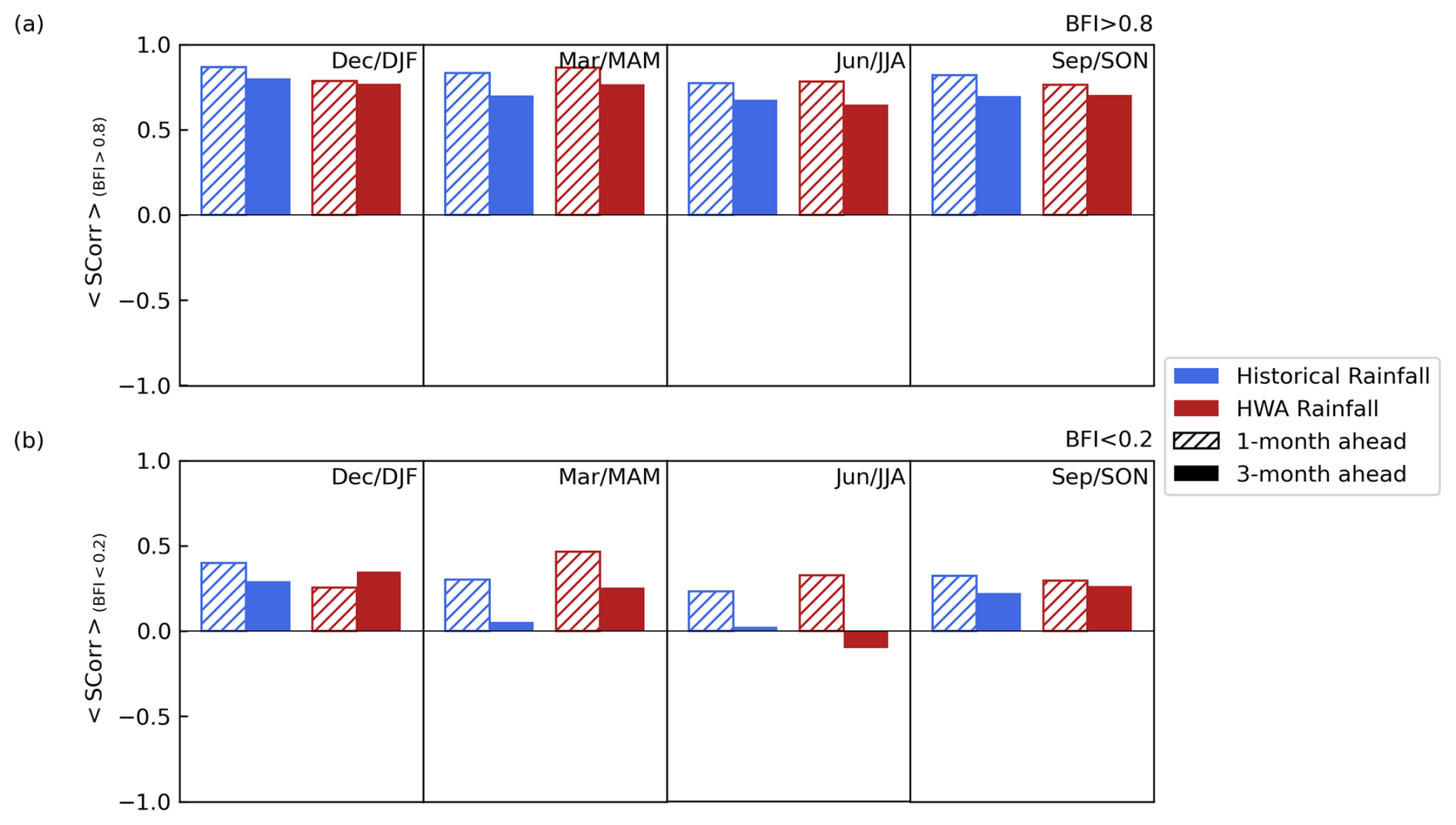
Figure 8 Pearson's correlation between river flow forecast ensemble mean and “ground truth” river flows for monthly (hatched) and seasonal (solid) forecasts generated using the WBM driven by historical ESP (blue) and HWA (red) rainfall forecasts. Shown are the correlations averaged over river cells with (a) high-BFI and (b) low-BFI.

Figure 8 shows the correlation between forecast ensemble mean and simulated “ground truth” flows for each of the four seasons, averaged over river cells with high BFI (top row) and low BFI (bottom row). The figure indicates the high performance of the forecast ensemble mean in regions where flows are dominated by subsurface stores (Fig. 8a), with only modest reductions in skill between monthly and seasonal forecasts. This suggests that hydrological memory is longer than three months in regions with high BFI. In addition, we observe that there is very little variation in the strength of the correlations (and thus forecast skill) over the year; this is because hydrogeology does not change seasonally.

By contrast, the low-BFI sample (Fig. 8b) includes only the catchments for which river flows are particularly sensitive to recent rainfall. The temporal variation in flow forecast skill in these catchments follows that of the rainfall forecasts, with the seasonal flow forecasts improved by HWA rainfall in winter, spring and autumn (see Fig. 3). In most cases, the correlation for a monthly forecast is stronger than that for the seasonal forecast that begins in that month, as the predictability of the rainfall declines with increasing lead time. The exception to this trend is the December/Winter skill, where rainfall predictability for both low and high BFI catchments is enhanced by the large-scale circulation patterns that correlate well over the later months of winter (West et al., 2021).

The analysis in this section has demonstrated the importance of both rainfall forecasts and hydrological initial conditions for reliable flow forecasts across Great Britain. However, the relative contribution of each source of forecast skill varies between regions where flows are dominated by subsurface stores and those sensitive to recent rainfall. Further efforts to improve the quality of UK hydrological forecasts by improving the rainfall forecasts should thus be directed at these regions where they can best complement the skill provided by hydrological initial conditions. The HWA forecasting approach offers the potential to do this by conditioning the ensemble on meteorological variables that correlate best with precipitation in these areas.

6 Conclusions

In this paper we have presented and assessed the performance of a new configuration of the G2G/WBM river flow forecasting scheme used in the UK Hydrological Outlook. The rainfall forecasts used to drive the hydrological modelling are now based on high-resolution historical weather analogues (HWA) conditioned on the large-scale circulation patterns predictions produced by GloSea6. This approach replaces an earlier scheme in which raw rainfall forecasts were spatially downscaled to the resolution of the hydrological model. We show that the HWA rainfall forecasts offer at higher spatial resolutions, skill that is comparable to that achieved over the UK by other models, but that some skill is lost compared to lower-resolution HWA forecasts. This results in forecasts that are, on average, marginally skilful in some seasons and regions. The best performance seen in winter in the north-west of Great Britain, attributable to the strong influence of the North Atlantic Oscillation. By contrast, in summer the rainfall forecasts are unreliable due to a lack of skill in the underlying GloSea6 forecasts.

We also examine the skill of the resulting river flow forecasts. We find that the G2G/WBM forecasting scheme performs well across much of Great Britain for most months and seasons, notwithstanding the marginal skill in the HWA rainfall forecasts. We compare our results to those found by Bell et al. (2017) for an earlier configuration of the forecasting system and conclude that HWA-based forecasts better predict the likelihood of low- and high-flow events in three of the four seasons. A small reduction in the skill score is found in autumn.

In line with previous work by Svensson et al. (2015), we found systematic variation in the sensitivity of river flows to recent rainfall in different parts of the country, with the north and west being most sensitive and the south-east being least. The work here has demonstrated this phenomenon at high resolution for ungauged catchments over the whole of Great Britain, extending the small sample of gauged catchments originally used by Svensson et al. (2015). These findings allow future improvements to rainfall forecasts and hydrological models to be targeted at the regions where they will have the most impact.

The analysis in this work has focused on only a relatively small number of available hindcasts, meaning that we have not been able to assess the performance of the forecasting scheme at detecting high-impact extremes (such as floods and droughts with > 20-year return periods). The hindcasts cover the period 1993–2017 and thus do not include more recent hydro-climatic extreme events and continuing changes in our climate. The argument could be made that the current operational performance may be different to that evaluated over the hindcast period. In Sect. S2 in the Supplement we briefly compare the performance of the operational scheme to that of the hindcasts and demonstrate that there is minimal evidence of a difference in performance.

Further work over the coming years will continue to improve both the weather forecasting and hydrological modelling components of the forecasting scheme. Initially, the atmospheric model ensemble size will be increased as more supercomputer resources become available. This should provide greater prediction skill and better constraints on the probabilistic forecast distribution, especially in the high-impact tails. We also plan to investigate whether we are now able to exploit the finer temporal resolution offered by analogue rainfall forecasts to replace the simplistic monthly-resolution water balance model currently used with a process-based representation of the water cycle (such as the Grid-to-Grid hydrological model). Across the UK Hydrological Outlook, there is a desire to make best use of the multiple available models by giving varying weight to different forecasting methods in proportion to their (seasonally- and spatially-varying) skill. Currently this is done subjectively by expert forecasters, but research is also underway into bias-correcting and statistically blending forecasts to better exploit each model's strengths. There are similar ambitions to explore multi-model ensembles to support seasonal weather forecasting in the UK.

The development of reliable 1 km rainfall and flow forecasts has recently enabled the release of monthly high-resolution seasonal forecasts for Great Britain through the Hydrological Outlook Portal (https://ukho.ceh.ac.uk/, last access: 29 September 2026). As seasonal hydrological forecasts continue to improve, they will become increasingly useful to a wide community of both professional and lay users.