Incorporating spatial heterogeneity into evapotranspiration estimates for bioretention basins

Green stormwater infrastructure (GSI) systems such as bioretention basins are frequently used in urban settings to reduce the amount of stormwater runoff entering combined sewer systems, thus protecting downstream waterbodies. Retaining stormwater in GSI allows it to infiltrate into the soil or return to the atmosphere via evapotranspiration (ET). While infiltration rates can be quantified with reasonable accuracy, methods of quantifying ET typically rely on models designed for homogeneous landcover like agricultural fields; the high spatial variation in factors including vegetation, light, and soil moisture renders estimates of ET from bioretention basins highly uncertain. To assess the influence of such variation on basin-scale ET and evaluate means of correcting for it, we quantified ET for a bioretention basin in Philadelphia, USA using three approaches: (1) an empirically-based model that incorporated chamber flux measurements of ET and accounted for heterogeneity in plant size, light conditions, and microtopography, (2) an empirical estimate of ET based on changes in soil moisture at a single location, and (3) a set of six conventional ET models that did not account for spatial heterogeneity. We further evaluated three methods of adjusting conventionally-modeled ET estimates to better align with those from the modeling approach based on chamber flux data. Our empirically-based model indicated that basin-scale, daily ET ranged from 0–6 mm d⁻¹, with temporal variation depending on weather conditions and time of year. A sensitivity analysis demonstrated that the spatial composition of plant height and shade strongly influenced basin-scale estimates. The soil moisture-based method found daily values to range from 0–4 mm d⁻¹, which more closely matched empirically based estimates for the sensor location than basin-scale estimates. Most conventional models overpredicted ET on average, though three models (Granger-Gray, Hargreaves-Samani, and Matt-Shuttleworth) were less sensitive to variation in atmospheric conditions and thus overpredicted ET at the low to middle part of the range but underpredicted ET at the upper end of the range. The muted response to atmospheric conditions limited the ability of additive or multiplicative adjustments (i.e., landscape coefficients) to improve agreement. In contrast, additive and multiplicative adjustments, as well as corrections accounting for shade, substantially improved agreement for the three models more sensitive to atmospheric conditions (Penman-Monteith ASCE, Penman-Monteith FAO, and Priestley-Taylor), with the strongest agreement resulting from additive adjustment of Penman-Monteith-derived estimates. Further analyses indicated that discrepancies between Penman-Monteith and empirical estimates could be attributed, in part, to differences in their treatment of wind speed, whereas accounting for soil-water limitation had little effect on these discrepancies. Our results highlight the importance of implicitly or explicitly accounting for spatial heterogeneity when quantifying ET, especially with respect to vegetation height and shade. For basins similar to our focal basin, this can be accomplished through the provided adjustments to conventional models. Additional calibration is required otherwise, but the growing availability of required data makes this increasingly viable.

1 Introduction

Green stormwater infrastructure (GSI) is a widely-used approach for managing stormwater in urban areas globally (McPhillips and Matsler, 2018; Li et al., 2019). Bioretention systems, such as rain gardens and bioswales, are a common type of GSI that incorporate both plants and soil media. These basins perform an array of hydrological functions such as allowing stormwater to infiltrate into the subsurface or return to the atmosphere via evapotranspiration (ET); these processes reduce peak flows as well as the volume of stormwater entering municipal stormwater systems (Pennino et al., 2016; Daniels and Yeakley, 2024). Reducing stormwater inputs to combined sewer systems can ultimately reduce the volume of combined sewer overflows into receiving water bodies (Hung et al., 2020; Joshi et al., 2021). An important contrast between infiltration and ET is that infiltration occurs predominantly during and immediately following storm events, whereas ET is much slower and acts throughout the period between events (Hess et al., 2021). As a result, ET more strongly determines if a basin's soil media is able to return to baseline moisture levels before the subsequent event (Johnston et al., 2020; Nasrollahpour et al., 2022).

The overall importance of ET to the removal of stormwater in bioretention basins is highly variable. In their review of ET in GSI, Ebrahimian et al. (2019) found that studies reported ET removing 19 %–84 % of influent stormwater, though a modeling-based analysis estimated ET below 5 % (Brown and Hunt, 2011), widening the range further. More recently, Huang et al. (2025) reported stormwater removal via ET ranging from near zero to almost 90 % across bioretention systems. Although this broad range encompasses systems operating under widely differing conditions, some of the variation can be attributed to well-established effects of climate, hydrology, vegetation, and system design. For example, removal via ET tends to decline with increasing hydraulic loading ratio (Huang et al., 2025) and also varies with vegetation and media characteristics (Nasrollahpour et al., 2022). However, the factors underlying this variation are often inadequately represented in ET estimates, particularly when heterogeneity occurs within individual bioretention systems. When bioretention basins are designed or evaluated (e.g., for regulatory compliance), ET is typically either disregarded or estimated using models (Traver and Ebrahimian, 2017). While modeling approaches are presumably less error-prone than ignoring ET altogether, conventional models were designed to inform agricultural irrigation practices and large-scale hydrologic budgets (Shuttleworth, 2007). They may therefore be inaccurate when used in urban settings with notably high heterogeneity in light, (micro)topography, and vegetation, all of which are fundamental to the energy and mass transfer equations on which ET models are based (Xue et al., 2025). Notably, standard implementations of energy-based models do not account for variation in plant size, which can be considerable at the scale of a bioretention basin. Depending on plant size and structure, the total leaf area overlying a portion of the basin's ground surface (i.e., leaf area index; LAI) may span several orders of magnitude. Although methods exist to help circumvent this limitation, such as multiplying by a landscape coefficient (K_L; Costello et al., 2000), they have not been evaluated in bioretention settings. A further challenge is that the most commonly-used models omit reductions in ET imposed by soil water limitation (McMahon et al., 2013), which are likely substantial in bioretention basins due to their fast-draining soil media, especially for periods between storms and in portions of basins with higher topographic positions. Solar radiation can also be variable at the basin-scale in densely urbanized environments, where buildings and other structures can cast significant shade. Given that weather and plant function drive ET, approaches that can accommodate the fine temporal scale resolution of ET may offer distinct advantages, though they often require larger quantities of input data (Ebrahimian et al., 2019; Skorobogatov et al., 2020).

Greater understanding of the accuracy and limitations of model-based ET estimates for use in bioretention basins would ideally come through comparison with measured or empirically-based estimates of ET. Empirical methods for quantifying ET exist but are rarely used in bioretention systems, either for research or in practice. This can be attributed to the fact that ET measurement systems require specialized equipment and can be labor intensive to operate. It is also possible to estimate ET from a water budget in which all other major fluxes are known (inflow, infiltration, and surface outflow; Li et al., 2009). However, methods such as static chambers, weighing lysimeters, and sap flow techniques are advantageous because they directly measure ET (or transpiration alone, in the case of sap flow) at fine spatial scales (Kool et al., 2014; Hamel et al., 2015). There are several examples of researchers applying these techniques to bioretention basins and other GSI (e.g., Denich and Bradford, 2010; Hess et al., 2017; Scharenbroch et al., 2016). However, few studies, if any, have examined the spatial and temporal variation of ET to evaluate the ability of conventional ET models to accurately estimate bioretention basin ET.

In this study, we applied plant physiological and geospatial techniques to a bioretention basin in Philadelphia, USA to answer two primary questions: (1) how can we incorporate the heterogeneous characteristics of bioretention basins into predictions of basin ET? and (2) how can we use our empirical observations to improve the accuracy of ET models that might be used when designing and assessing bioretention basins? To address the first question, we collected ET measurements across a gradient of zones within the basin over the course of a growing season, characterized the distribution of plants, shading, and topography in the basin, and modeled ET through the growing season using the empirical data. We also assessed the sensitivity of this empirical model to several input parameters to examine the implication of excluding or oversimplifying spatial variability in bioretention ET modeling. For the second question, we compared our results to conventional ET estimation methods (e.g., Penman-Monteith) and calculated coefficients to tailor those estimates to bioretention basins. Empirically-based ET models tailored for bioretention basins can both be used by designers to better apportion credit for ET-based volume reduction and adjust design choices such as the location of larger versus smaller plants to maximize ET.

2 Materials and Methods

2.1 Study site

This study focused on a bioretention basin in Philadelphia, Pennsylvania, USA (39.96662° N, 75.13404° W). It is designated GR2 SMP A (hereafter, Basin A) and was constructed in 2016 as part of an effort to reduce combined sewer overflows into the Delaware River. It is situated in a mixed-use neighborhood (residential and commercial) but is adjacent to an elevated portion of the Interstate 95 highway (I-95, Fig. 1a). The annual average daily traffic volume of this portion of I-95 is ∼ 198 000 vehicles per day (PennDOT, 2022). An approximately 2695 m² portion of the roadway and shoulder drains into the basin via two inlet pipes, though some runoff also enters via a sloped structure between two segments of the highway wall. The basin is approximately linear (148 m in length and 5 m in width) and has a trapezoidal cross section (∼ 1.5 m depth). The middle 44 m of the basin's length contains a rock-filled gabion that causes the basin sections at either end to remain hydrologically separated except during extremely large storms. For the purposes of this study, we focused only on the portion of the basin to the southwest of the gabion (Fig. 1a). During construction, urban fill was replaced with an engineered soil medium with a gravelly loamy fine sand texture (as per USDA) to a depth of approximately 0.5 m. Prior to planting, the basin's flanks (i.e., sloped sides) were covered with landscape fabric. Vegetation is predominantly composed of graminoids, herbaceous perennials, and shrubs. Annual and perennial weeds are also present but are removed several times during each growing season. Most vegetation reaches < 1 m in height when mature but some plants are taller, including a cluster of shrubs growing along the highway wall near the inlet (∼ 4 m; Fig. 1b). The vast majority of plants are deciduous and therefore leafless from late fall through early spring. Additional site characteristics were provided by Ampomah et al. (2023), Caplan et al. (2024), Pope et al. (2025), and Shakya et al. (2023).

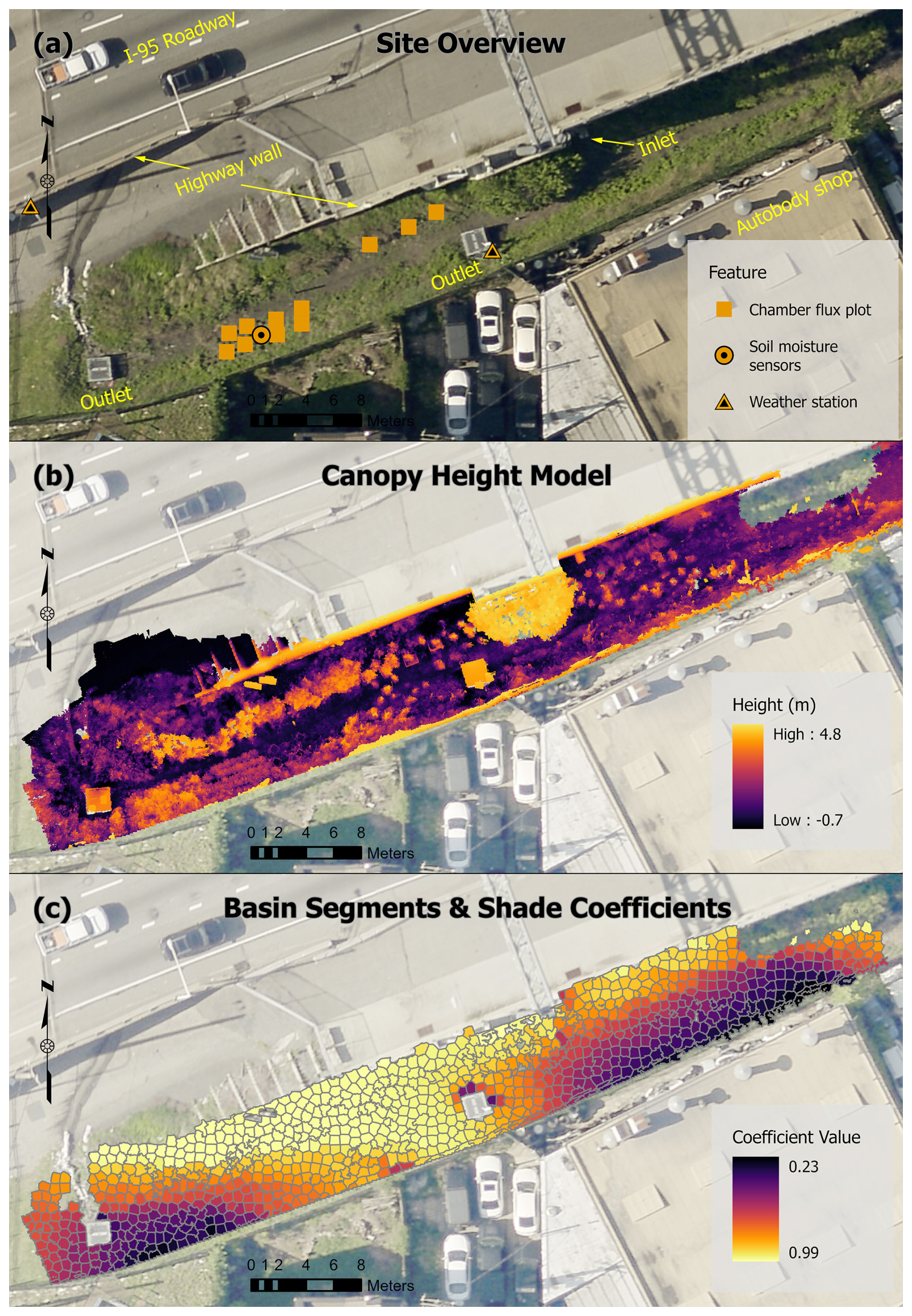
Figure 1 (a) Aerial view of the lower portion of Basin A, which served as the focal site for this study. Symbols indicate where ET, weather, and soil moisture data were measured. (b) Distribution of plant canopy heights; color scale is non-linear. (c) Distribution of shade coefficients for an example day (day of year = 180) at the segment scale. The aerial photograph was taken in 2022 by the City of Philadelphia.

2.2 Chamber flux measurements

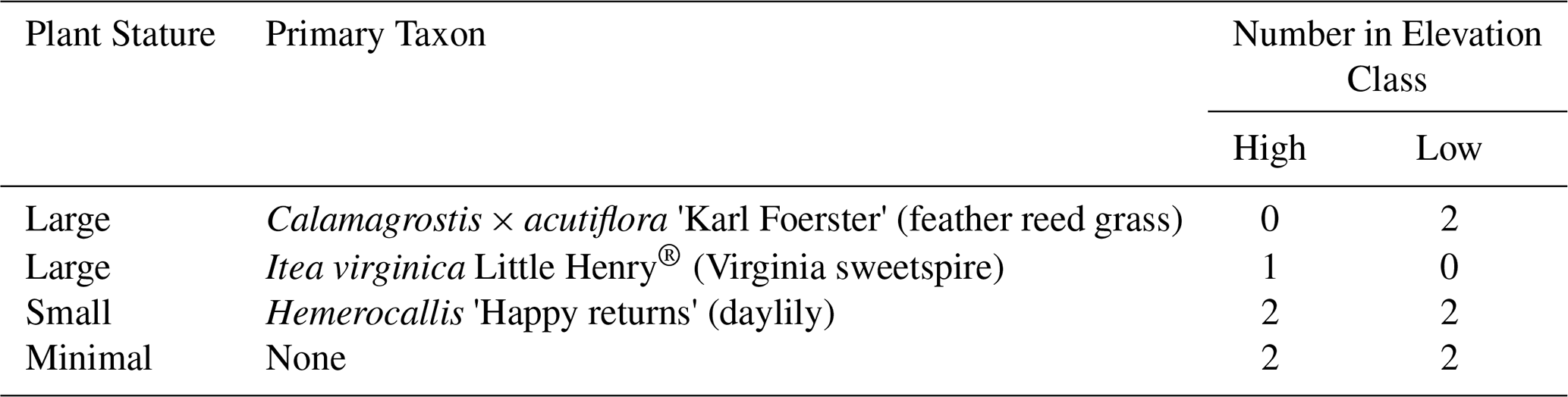
We measured ET rates at 11 fixed locations (i.e., plots) within the lower portion of Basin A. Eight of the plots were established such that half were at high or low topographic positions (to capture soil moisture variability within the basin), while half from each group were either in a cluster of small stature vegetation or in a minimally-vegetated area (Fig. 1a). Three additional plots were in an area with larger vegetation. The eight plots containing small or large vegetation were centered on a single, dominant plant (Table 1, Figs. 1a, S1 in the Supplement), though small weeds were also typically present. The minimally vegetated plots contained bare ground along with small weeds.

Table 1 Characteristics of the plots in the study basin that were used for ET measurements.

Atmospheric conditions and soil moisture were intentionally variable across the seven measurement dates, which spanned June through October 2019. Plants were full-sized through this period, eliminating the influence of seasonal canopy size variation on our data. In particular, we targeted several dates with little antecedent rainfall and other dates that followed storm events. All measurement dates were rain-free to ensure intercepted rainwater evaporating from leaf surfaces would not confound ET measurements. Air temperature and humidity also varied considerably across the growing season, though we also captured variation in these parameters by taking measurements multiple times through each day (see below).

ET measurements were made using the closed dynamic chamber method, in which all vegetation and soil within a plot are temporarily enclosed in a fixed-volume chamber to measure the accumulation of water vapor. Although more commonly used to measure carbon fluxes (e.g., Bansal et al., 2023; Geoghegan et al., 2018; Norman et al., 1997), the method has been successfully applied to water flux measurements as well (Garcia et al., 2008; Hamel et al., 2015; Luo et al., 2018). Custom-made collars were set into the soil at the beginning of the field season, demarcating plot boundaries (Fig. 1a). The upper faces of collars were square and approximately parallel to the basin's bottom. Plots with minimal and small-stature vegetation had collars with upper surfaces of the same dimensions (52 × 52 cm; n=8), while those used for larger plants were substantially greater (92 × 92 cm; n=3). We measured ET at each plot five to six times per day, typically between 800 and 1900 h, at approximately 90 min intervals. For each measurement, we first attached a transparent chamber and lid to the abovementioned collar (Fig. S1). We then measured water vapor in the enclosure once per second using an ultra-portable greenhouse gas analyzer (UGGA; Los Gatos Research, San Jose, CA, USA) that was connected to the chamber using a pair of flexible tubes (4.3 m long). Calculating ET required isolating the linear portions of time series recorded while chambers were closed and performing linear regression to determine the rate of water vapor accumulation. After excluding cases with insufficient data quality (∼ 17 %), our dataset contained 302 usable ET measurements. Additional details on chamber flux measurements and associated calculations are provided in Sect. S1.1 in the Supplement.

2.3 Environmental data

Weather data were measured at two locations (Fig. 1a). One was elevated above the highway and provided air pressure and total solar radiation for the entire study period at 5 min intervals. The second was located within Basin A and provided an incomplete set of temperature, relative humidity, and wind speed data, also at 5 min intervals. To infill missing temperature and relative humidity data, we obtained estimated values for Basin A from the DarkSky weather data service (http://www.darksky.net, last access: 1 March 2023), which uses spatial interpolation to generate hourly time series at a specified location. DarkSky values were interpolated to the 5 min interval using the Stineman (1980) method (via R library imputeTS). The resulting time series were well-correlated with the partial datasets measured in the basin itself ($R_{\mathrm{Temp}}^{\mathrm{2}}=\mathrm{0.98}$, $R_{\mathrm{Rh}}^{\mathrm{2}}=\mathrm{0.95}$).

Volumetric soil water content (VWC) was measured using TEROS 12 sensors (Meter Environment, Pullman, WA, USA) installed on the south flank of Basin A, approximately 40 cm above the basin floor (Fig. 1a). The sensors were a subset of those used in a separate study (Pope et al., 2025) and were within 1 m of each other. Sensors were positioned at 5, 10, 30, and 60 cm depth, with the latter three arranged in a vertical profile. For empirical modeling of ET (see Sect. 2.5), we used the mean VWC from 5 and 10 cm depths since these measurements most directly depicted near-surface moisture conditions. Missing values in the 10 cm time series were first interpolated from concurrent measurements recorded by nearby sensors, yielding complete data for 137 d (8 June through 22 October). The sensors at 10, 30, and 60 cm provided a soil moisture time series spanning the soil profile and were used in analyses requiring data from multiple depths (see Sect. 2.7 and 2.8). Profile data were missing for three of the days included in the empirical-model time series as they could not be accurately interpolated (n=134 d).

Because the air's influence on ET derives from the combined effects of air temperature and relative humidity, we computed vapor pressure deficit (VPD) to describe evaporative demand with a single metric. The calculation of VPD was made using VPD = VP_sat (1 − Rh), where VP_sat is the saturated vapor pressure of the air (a function of its temperature; we used the equation provided by Wagner and Pruss, 1993) and Rh is the relative humidity.

2.4 Basin spatial characterization

We characterized the basin's topography, as well as its spatial heterogeneity in vegetation height, using a combination of terrestrial LiDAR and drone-based photogrammetry. First, we generated a 3D point cloud with Trimble TX5 3D terrestrial laser scanner (Trimble Inc., Sunnyvale, CA, USA), which was georeferenced and edited to yield a bare earth cloud model; this was subsequently converted to a grid (the final DEM). In addition, we generated a digital surface model (DSM) from drone-based photographs using structure-from-motion (methods followed Alonzo et al., 2020). Vegetation height was determined by subtracting the DEM from the DSM (Fig. 1b). The DEM data further enabled us to create a set of polygons demarcating topographic position within the basin; we classified areas as either “lower” (the bottom where stormwater was intended to flow and infiltrate) or “upper” (the basin's flanks). Additional details are provided in Sect. S1.2.

We characterized spatial and temporal variation in solar radiation by adjusting the empirical time series of unshaded irradiance (from the sensor above the highway) with correction factors that accounted for how the site was shaded by surrounding features. The primary tool used to generate these correction factors (which we call shade coefficients) was the Area Solar Radiation calculator in ArcMap 10.8 (ESRI, Redlands, CA, USA). This tool uses a DEM as input to quantify solar radiation for each pixel at hourly or coarser intervals. Because we were interested in the shading effects of features such as the highway wall, nearby buildings, and a billboard, we generated a DEM from an aerial LiDAR dataset collected over the Philadelphia region in 2018 (City of Philadelphia, 2018); it had a 30 cm resolution. We worked with data covering an area large enough to include all features that could potentially shade the study site (238 × 167 m). For each pixel in this DEM, the Area Solar Radiation calculator determined total direct and diffuse solar radiation for each day of the study period but did so in the absence of clouds. These were used to compute shade coefficients (C_p,t) for each pixel (p) on each day (t) throughout the study period:

$$\begin{array}{}\text{(1)}& C_{p,t}={\displaystyle \frac{{\mathrm{Direct}}_{p,t}+{\mathrm{Diffuse}}_{p,t}}{{\mathrm{Direct}}_{u,t}+{\mathrm{Diffuse}}_{p,t}}},\end{array}$$

where u indicates the pixel containing the unshaded sensor. Shade coefficients could reach as high as one if there was no shading from nearby structures but typically ranged from 0.75 to 0.95; they almost never fell below 0.3 due to diffuse radiation (Fig. 1c). The matrix of shade coefficients was multiplied by the empirical time series from the unshaded sensor to yield location-specific daily time series of solar radiation that included the shading effects of both clouds and structures surrounding the site.

In order to make the computation of ET tractable across Basin A, we used object-oriented image analysis to aggregate predictor variables to roughly the plant scale (Blaschke, 2010). This process segmented the basin into polygons (n=967) with relatively homogenous vegetation height, specifically using the simple linear iterative clustering algorithm (Achanta et al., 2012; details in Sect. S1.2). We then aggregated pixel-scale values of the shade coefficient (Fig. 1c), topographic position, and canopy height to the segment scale using the zonal median; segment-scale values were used for all subsequent analyses.

2.5 Empirical model of ET

We developed a statistical model of ET to make it possible to estimate ET while incorporating temporal and/or spatial variation in plant height and the environmental conditions described above. The response variable was ET as measured by chamber flux; high-quality data from all 11 plots and 7 dates were included (n=302). Predictor variables included topographic position (categorical, where 0 = lower basin and 1 = upper basin) and the following continuous variables: plant height, vapor pressure deficit, solar radiation, and mean soil moisture from 5 and 10 cm depths. Values of these variables corresponding to the locations and times of chamber flux measurements were extracted from larger datasets for use in the statistical model. The model also included all possible two- and three-way interaction terms among the five predictor variables as well as random intercepts for plot identity, measurement date, and their interaction. Including topographic position as a binary variable allowed the influence of continuous variables to differ between the basin's bottom vs. flanks through interaction terms; this was expected to be particularly important for soil moisture. Higher-order interaction terms were not included in the final model since they had poor explanatory power and would have been nearly uninterpretable. A square-root transformation was applied to the response variable (ET) to improve the normality and homoscedasticity of residuals (Fig. S2a, b).

We fit the model using restricted maximum likelihood estimation. This was done with functions from the lme4 library (Bates et al., 2015) in R v4.4.2 (R Project for Statistical Computing, Vienna, Austria). Continuous predictor variables were standardized (centered and divided by their standard deviations) prior to model fitting, allowing the magnitudes of the resulting coefficients (β) to indicate the relative effect sizes of each term. Model fit was assessed using marginal and conditional coefficients of determination ($R_{\mathrm{m}}^{\mathrm{2}}$ and $R_{\mathrm{c}}^{\mathrm{2}}$, respectively; Nakagawa et al., 2017). In this context, $R_{\mathrm{m}}^{\mathrm{2}}$ represents variance explained only by the fixed effects while $R_{\mathrm{c}}^{\mathrm{2}}$ represents variance explained by the fixed and random effects together. The difference between $R_{\mathrm{m}}^{\mathrm{2}}$ and $R_{\mathrm{c}}^{\mathrm{2}}$ therefore reflects the variation accounted for by random effects. Type II Wald χ² tests were used to determine which coefficients were statistically different from zero (using the car package; Fox and Weisberg, 2019). We focused our interpretation on significant terms (p < 0.05) with relatively large effects, although we retained all terms in the model to preserve model hierarchy.

We used the parameterized ET model to predict ET for each basin segment; these had unique topographic positions, plant heights, and shade coefficients but all followed the same time series of solar radiation, vapor pressure deficit, and soil water content. ET was estimated at 5 min intervals at the segment level and then summed for each day. Predictions spanned 8 June to 22 October (n=137 d), corresponding to the period with complete near-surface soil moisture data. Daily ET for each segment was multiplied by segment area, summed across all segments, and divided by total basin area to obtain daily, basin-scale ET. Basin-scale ET was converted from mmol m⁻² d⁻¹ to mm d⁻¹ using the molar mass and density of water (18 g mol⁻¹ and 1 g cm⁻³, respectively). Night was excluded since our empirical model was parameterized only under daylight conditions; this means that values are slightly lower than they would be if ET estimates spanned 24 h periods (likely ∼ 5 %; Groh et al., 2019).

2.6 Sensitivity analysis

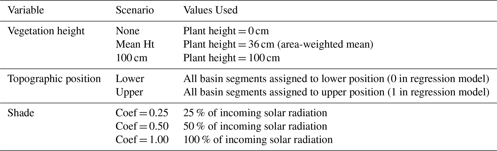
We assessed the importance of accounting for spatial heterogeneity when determining basin-scale ET by comparing initial model estimates to those from additional calculations that did not account for it. Specifically, we determined the sensitivity of the whole-basin empirical model to plant height, topographic position, and the shade coefficient, calculating basin-scale ET under eight scenarios in which each of those variables took on fixed values (Table 2). We then summed daily ET values across the study period for each scenario and used total ET through the 137 d focal period as the basis of comparison.

Table 2 Variables used to test the sensitivity of the whole-basin empirical model.

2.7 Comparison to soil moisture-based estimates

To provide an empirical point of comparison for our ET model, we calculated ET from a soil moisture time series. This is a relatively simple method previously developed for estimating ET in bioretention systems (Hess et al., 2021), though it does not account for spatial variability unless measurements are made at multiple locations. Data came from the set of soil moisture sensors at 10, 30, and 60 cm depth. For each storm event during the study period, we first identified the period of rapid decline in soil moisture values corresponding to gravimetric flow draining the soil. We isolated data after these periods, namely when soil moisture was held by capillary tension and continued to decline, though at a slower rate. This phase of soil moisture loss can be attributed exclusively to ET in most cases (Bowman and King, 1965; Hess et al., 2021). To calculate ET, we assumed that volumetric water content in the top 10 cm equaled the sensor reading at 10 cm, and linearly interpolated between the other sensor depths to estimate total water content in the upper 60 cm. We then calculated the rate of ET as the net change in total water content over time, isolating each day during the study period with complete data (n=68).

We compared soil moisture-based ET with both basin-scale empirical-model estimates and local empirical-model estimates for the four spatial segments near the soil moisture sensors. Daily ET rates for these segments were converted from mmol m⁻² d⁻¹ to mm d⁻¹ as described above and the area-weighted average was computed. Agreement was quantified using concordance correlation coefficients (CCC; Lin, 1989). CCC evaluates not only how two datasets align with each other but how close they come to perfect agreement (i.e., a 1 : 1 line). Like other correlation coefficients, CCC ranges from −1 to 1, but here 1 indicates perfect concordance, 0 indicates no concordance, and −1 indicates perfect discordance. We additionally calculated root mean square errors (RMSE) and compared the paired absolute differences between soil-moisture-based ET and both local and basin-scale estimates using a Wilcoxon signed-rank test.

2.8 Comparison to conventional models

We estimated daily ET for the focal section of Basin A using meteorological data applied to six commonly-used ET models (i.e., conventional models) through the R library Evapotranspiration (Guo et al., 2016). These included models describing potential ET (Priestley-Taylor (PT)), reference ET (ET₀; Hargreaves-Samani (HS), Matt-Shuttleworth (MS), as well as both the FAO (Food and Agriculture Organization of the United Nations) and ASCE (American Society of Civil Engineers) variants of Penman-Monteith (PM)), and “actual” ET (Granger-Gray (GG)). Using these six conventional models, we estimated ET at a daily timescale from 8 June to 22 October. Table S1 summarizes the input variables and constants used in these model runs.

Our primary model estimates used the raw time series of solar radiation, with the implication that they did not include the influence of shade from nearby structures, unlike our empirical-modeling approach. We therefore additionally generated estimates using a solar radiation time series adjusted for the effect of shade from structures. This required calculating shade coefficients that could be applied to the basin as a whole for each day of the study period. To do this, we first calculated the area-weighted mean of shade coefficient values across all basin segments; this was done for each day of the study period. Then we multiplied the total solar radiation value for each day by the corresponding shade coefficient, yielding the adjusted time series. CCC values were the primary means by which we compared ET estimates from conventional models to those from our whole-basin empirical model.

We also evaluated whether wind speed or soil-water limitation contributed to differences between conventional and empirical ET estimates. For wind speed, we used linear regression to determine if the magnitude of these differences (i.e., bias) exhibited a systematic relationship with wind speed. If so, it would indicate that not explicitly accounting for variation in wind speed in our empirically-based model contributed to discrepancies with one or more of the conventional models. For soil-water limitation, we adjusted conventional modeling estimates of ET with an FAO-56-style water-stress coefficient (K_S; Allen et al., 1998) and evaluated the effects of incorporating soil moisture stress on bias (specifically, conventional minus empirical ET) and concordance between conventional and empirical ET estimates. K_S values were derived from the profile-based soil moisture time series and water retention characteristics (Shakya et al., 2023), using three plausible effective rooting depths (20, 30, and 40 cm; additional details in Sect. S1.3).

2.9 Landscape coefficients

Landscape coefficients (K_L) are used to adjust reference evapotranspiration rates (ET₀) so they better reflect ET in ornamental or landscaped settings (Costello et al., 2000). Like crop coefficients used in agricultural settings, K_L values are multiplicative and can be considered a form of bias correction. K_L has been determined traditionally by observing the type of species, planting density, and microclimate conditions at a site and applying guidelines from Costello et al. (2000). More recently, K_L values have been determined by comparing measurements of actual ET with reference ET (Sun et al., 2012), facilitating their determination for a wide array of landscaped settings and plant combinations.

We used the latter approach by comparing our daily-scale, basin-wide empirical ET calculations (ET_emp) with the ET estimates from the six conventional models described above (ET_ref). Specifically, we fit the following equation using a trust-region-reflective algorithm implemented via the Matlab function fit (Coleman and Li, 1994, 1996):

$$\begin{array}{}\text{(2)}& {\mathrm{ET}}_{\mathrm{emp}}=K_{\mathrm{L}}\times {\mathrm{ET}}_{\mathrm{ref}}\end{array}$$

where ET_emp and ET_ref were both calculated at a daily interval using weather data from 8 June to 22 October. We then multiplied K_L by ET_ref to generate corrected, daily-scale ET estimates, which we compared to ET_emp using the CCC.

2.10 Additive correction factors

We also tested additive correction, a simple approach that can be used to adjust for model bias when it is consistent across a sufficiently wide range of values. It has been applied to estimates of various meteorological parameters, including ET (Paredes et al., 2018), although it has the potential to yield negative values when the correction exceeds the uncorrected estimate. Such values would have little influence on estimates aggregated over longer periods as long as they are small and infrequent. To determine the correction factors, we first regressed each set of ET_ref estimates against ET_emp and then subtracted the fitted intercept from each ET_ref estimate when the intercept was positive. As with the landscape coefficient adjustments, we used the CCC to assess how additive corrections improved ET_ref.

3 Results and Discussion

3.1 Empirical ET patterns and model

On all seven measurement dates, ET followed the expected diurnal pattern: it was near-zero in the early morning, peaked in the mid-afternoon, and declined in the evening (Fig. 2). However, the amplitude of this oscillation varied considerably from day to day. It was notably muted for all plots on 27 August, when temperature and VPD were elevated and there had been little antecedent precipitation (Fig. 3). The diurnal amplitude was also muted (though to a lesser degree) on 14 October, likely due to the dry September that preceded it, as well as temperature and solar radiation declining towards the end of the season.

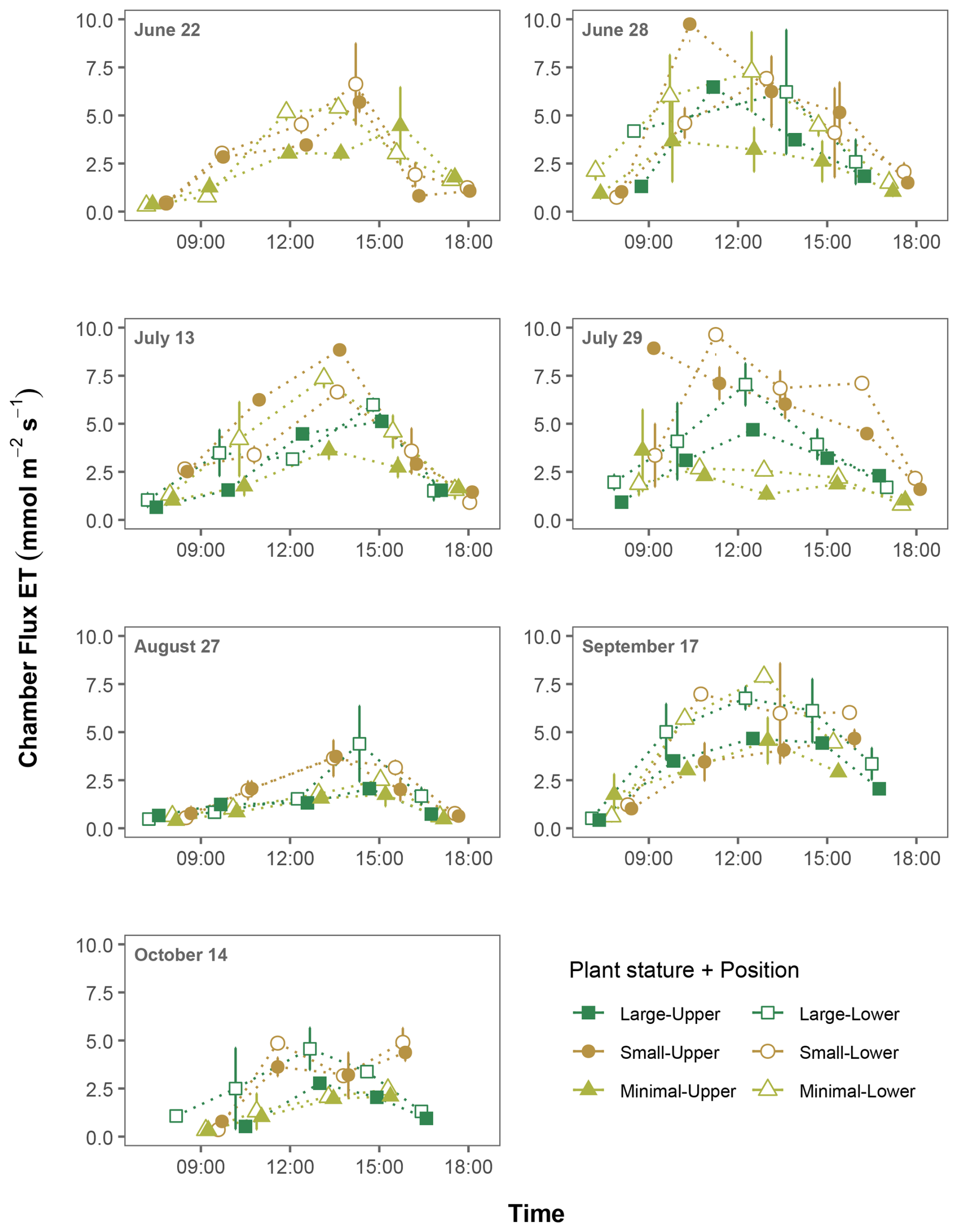
Figure 2 Plot-scale evapotranspiration rates in Basin A measured using flux chambers. Mean rates (±SE) for each combination of plant stature and position are shown. Points without error bars either represent single points or their SEs are hidden by symbols.

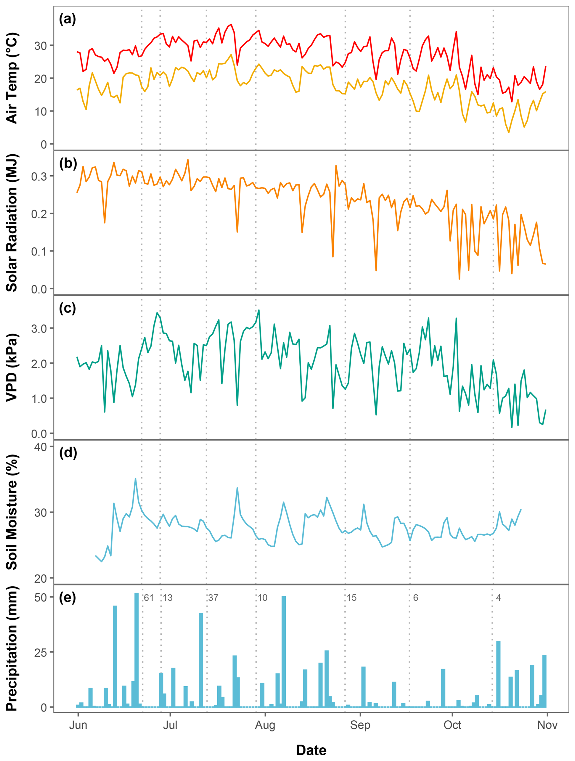
Figure 3 Environmental conditions at the field site through the study period. Shown are (a) daily maximum and minimum air temperatures, (b) daily maximum solar radiation and (c) vapor pressure deficit (VPD), (d) mean soil moisture at 5 cm depth, and (e) total precipitation. Vertical dotted lines indicate dates of ET measurements while numbers in (e) are antecedent precipitation index values (Kohler and Linsley, 1951) calculated using a 10 d window.

The statistical model was able to explain most of the observed variation in ET across measurement dates and plots ($R_{\mathrm{m}}^{\mathrm{2}}=\mathrm{0.65}$, $R_{\mathrm{c}}^{\mathrm{2}}=\mathrm{0.78}$; Fig. S2c, d), with its largest coefficients (β, Table 3) realistically encapsulating environmental and plant processes. For one, ET increased particularly strongly with solar radiation and VPD (β=0.393 and β=0.375, respectively). Also, ET was lower in the upper part of the basin ($\mathit{\beta }=-\mathrm{0.158}$), likely because flooding by stormwater runoff was less frequent higher on basin flanks. Further, the effect of VPD on ET intensified when soil media was wetter (β=0.181), reflecting the greater ability of evaporative demand to drive ET when unsaturated soil contains more water. Less intuitively, the effect of solar radiation on ET appeared to weaken when soils were wetter ($\mathit{\beta }=-\mathrm{0.089}$), though this can be explained by reduced evaporative efficiency and/or plants limiting transpiration under (near-)saturated conditions. However, this relationship differed by topographic position (β=0.112); on basin flanks, greater moisture enhanced the ability of solar radiation to promote ET, whereas in low-lying areas, greater moisture levels dampened this response, likely due to (near-)saturation restricting water loss from plants and soil.

Table 3 Coefficients (β) and Type II Wald χ² tests for the empirical model of ET from chamber flux measurements. The response variable (ET) was square-root transformed and continuous predictor variables were standardized prior to fitting; topographic position was coded as a binary variable and not standardized. Topo = topographic position, where 0 =  lower basin and 1 = upper basin; Plant Size = plant height; VPD = vapor pressure deficit; Solar Rad = solar radiation; VWC =  volumetric water content.

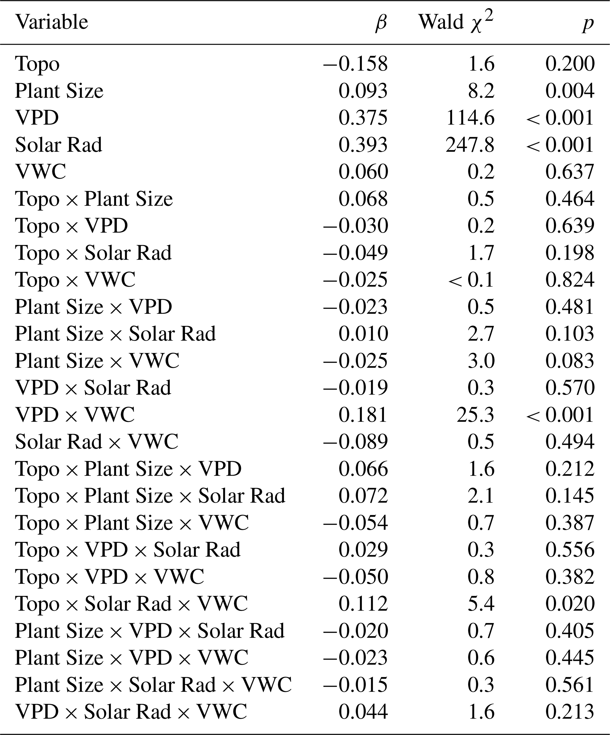
ET was also greater in locations where plants were taller (β=0.093), reflecting the ability of greater leaf cover per unit ground area (a.k.a. leaf area index, or LAI) to raise ET (Steduto and Hsiao, 1998). The fact that this effect was not larger was likely due to available energy constraining the extent to which greater LAI could increase ET, as well as larger plants shading the soil surface more completely, inducing a tradeoff between soil evaporation and transpiration. Another factor may have been the fact that larger plants tended to have small or no other plants around them, diminishing LAI at the plot level. Previous observations of similar leaf-level transpiration rates among the three focal species (Toran et al., 2017) suggest that differences in physiological rates had a minimal influence on the relationship between plant size and ET.

3.2 Basin-scale empirical ET model

At the basin scale, peak ET exhibited the expected seasonal decline, progressing from about 6 mm d⁻¹in early-and mid-summer to around 1 mm d⁻¹ by mid-autumn (Fig. 4a). However, ET was well below peak values on most days, likely due to limitations associated with weather (especially reduced solar radiation on cloudy days and reduced VPD on cool or humid days). The clearest spatial pattern was that ET was elevated in areas with the tallest plants. This was most notable for a cluster of shrubs adjacent to the highway wall (Fig. 4b). However, plants in other areas were relatively tall (i.e., > 100 cm), and although they exhibited modest ET, values were smaller than expected. This was likely due to the effects of shade from two buildings and a billboard immediately to the south of the basin. Given that the highway wall was to the north of the basin, its shading effects were minimal. There was also relatively little variation in ET associated with topographic position, likely because plants tended to be shorter in the low-lying portion of the basin but taller on the flanks and surrounding areas.

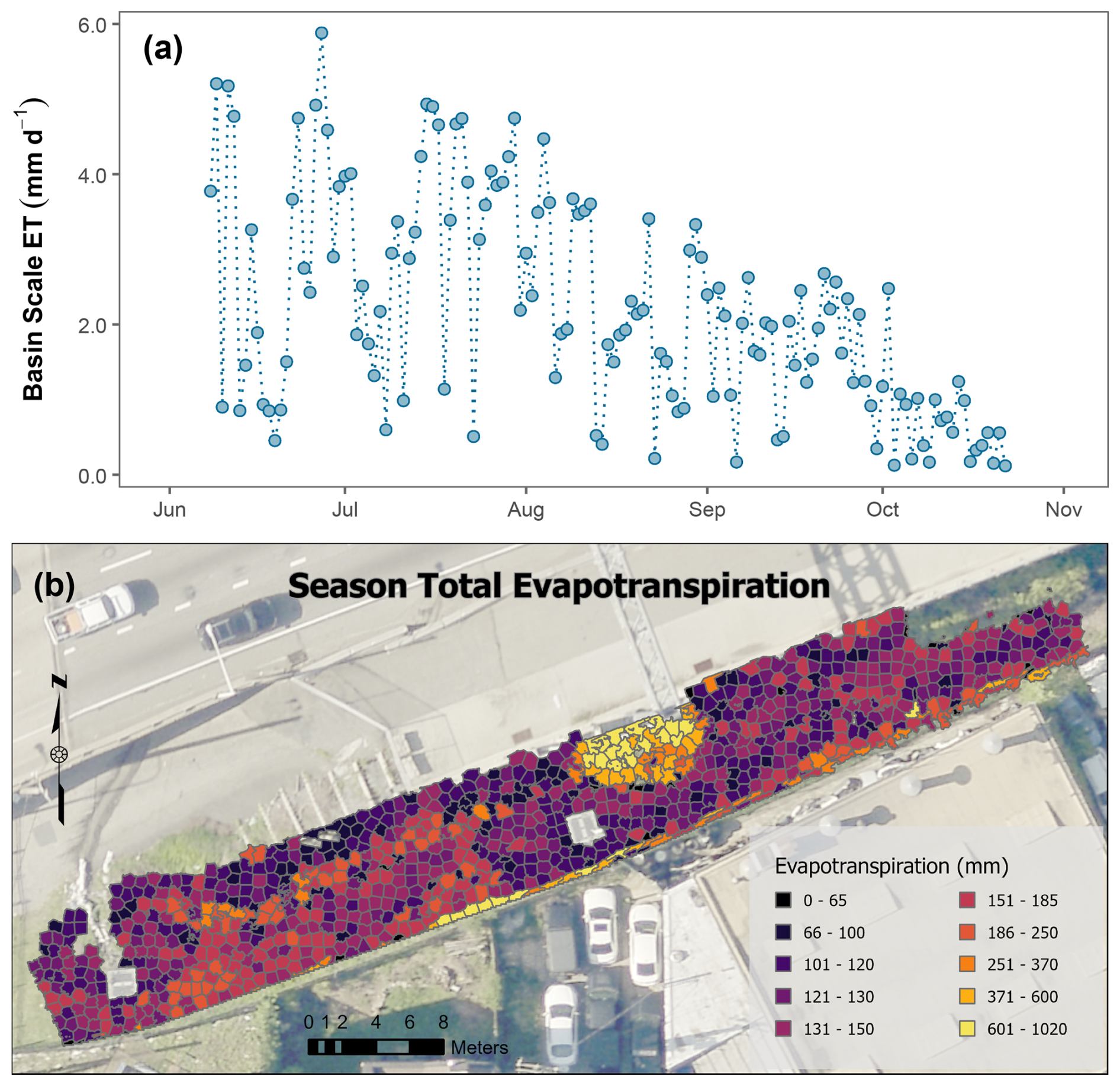
Figure 4 (a) Daily ET estimated by the empirically based model for the whole basin spanning the focal period (8 June to 22 October) and (b) season-wide ET estimated by the model for each basin segment. The aerial photograph was taken in 2022 by the City of Philadelphia.

3.3 Sensitivity analysis

Total ET through the study period, when calculated at the basin scale, was most sensitive to plant height. It fell well below the baseline (−41 %) with all plant heights set to zero but rose to +60 % with all plant heights set to 100 cm (Fig. 5). When we applied the area-weighted mean height (36 cm) to the entire basin, the season-wide estimate of ET was still reduced, at −13 %. Treating all segments as having upper or lower topographic positions had little influence on seasonal ET, changing it by −3 % and +0.5 %, respectively (Fig. 5). In contrast, quantifying ET under the scenario that no structures shaded the basin yielded an 11 % increase in season-wide ET. This decreased to −48 % when we applied a shade coefficient of 0.25 (i.e., 25 % of incoming solar radiation reaching the basin) and −32 % with a shade coefficient of 0.5.

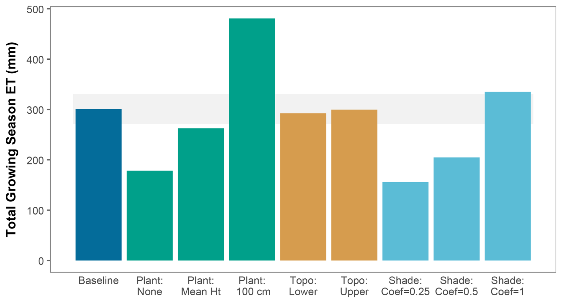
Figure 5 Comparison of whole-basin empirical ET estimates for the sensitivity scenarios described in Table 2. Total growing season ET includes all dates from 8 June through 22 October. The horizontal grey bar indicates ±10 % of the baseline model results (original basin conditions). Plant, Topo, and Shade refer to scenarios in which all basin segments were assigned the same vegetation height, topographic position, and incoming solar radiation values, respectively (details in Table 2).

A study of ET in experimental bioretention cells (Nocco et al., 2016) likewise found that ET varied strongly with vegetation type, specifically with prairie plants (forbs and graminoids) > shrubs > turfgrass > bare soil. In that study, prairie plants had similar heights but a much higher density than shrubs (13.6 plants m⁻² vs. 1.1 plants m⁻²), likely meaning that LAI primarily drove the differences in ET.

3.4 Comparison to soil moisture-based ET estimates

Soil moisture-based ET estimates agreed moderately well with basin-scale, empirically-modeled ET (CCC = 0.63; Fig. 6a). Further, the two approaches yielded ET rates that spanned a similar and reasonable range, suggesting that the empirical model produced reasonable estimates of ET. Nonetheless, when ET exceeded 2 mm d⁻¹, soil moisture-based ET often yielded lower ET rates. However, there were smaller differences between soil moisture-based ET and empirical-model estimates for the segments near the sensors (Fig. 6b). Although CCC was also 0.63, RMSE decreased from 1.15 to 0.92 mm d⁻¹, and absolute differences were significantly lower for the local estimates (Wilcoxon signed-rank test, p=0.009).

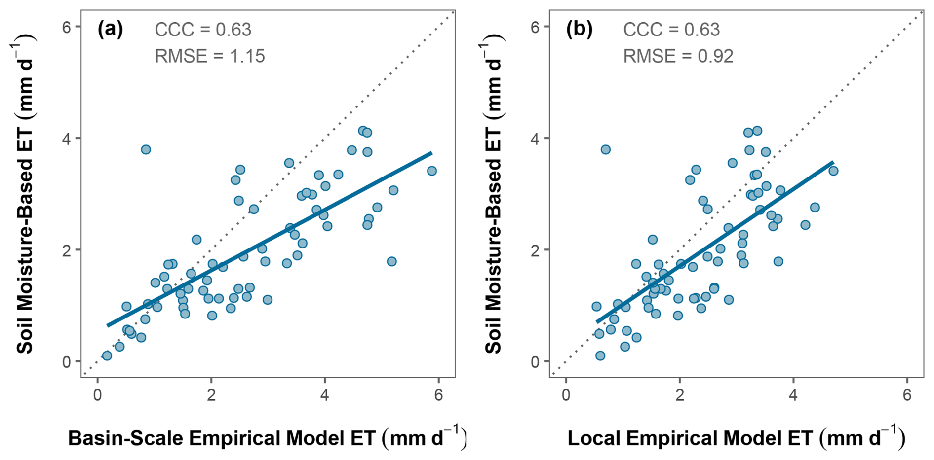
Figure 6 Daily soil moisture-based ET compared with empirical-model estimates (a) at the basin scale and (b) in the area near the soil moisture sensors. Dotted lines depict 1 : 1 relationships. CCC = concordance correlation coefficient; RMSE = root mean square error (n=68).

While the soil moisture-based method has been validated using weighing lysimeters set up to mimic stormwater cells (Hess et al., 2021), comparisons among observational methods have demonstrated that ET quantification in GSI systems has substantial uncertainty (Ouédraogo et al., 2023). It is therefore not possible to definitively determine which approach more accurately reflected true, basin-scale ET. However, given that the soil moisture sensors used here were installed on the flank of the basin rather than the bottom, the soil moisture-based approach could be expected to underestimate basin-scale ET. The reduction in RMSE for the local empirical-model estimates supports this interpretation and provides additional evidence that the empirical model was capable of capturing spatial variation in ET within the basin. Given that the soil moisture-based approach can be influenced by the placement of the soil moisture sensors, especially in basins with high spatial heterogeneity, combining data from multiple sets of sensors would likely improve its accuracy considerably.

3.5 Comparison to conventional ET models

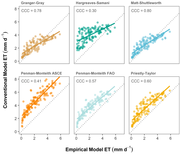
In the absence of correction factors, there was moderately strong agreement between the basin-scale values generated by our empirical model and those from conventional ET models. The MS and GG models had the highest agreement (CCC_orig= 0.80 and 0.78, respectively; Fig. 7); however, both overestimated lower ET rates and underestimated higher ET rates. Further, the PM-ASCE, PM-FAO, and PT models consistently overestimated ET relative to our empirical model, leading to an offset that lowered CCC values (CCC_orig= 0.41, 0.57, and 0.60, respectively; Fig. 7). The HS model also overestimated ET and had the poorest agreement of the six models (CCC_orig= 0.30), although it produced estimates close to those from the empirical model for ET rates above 4 mm d⁻¹.

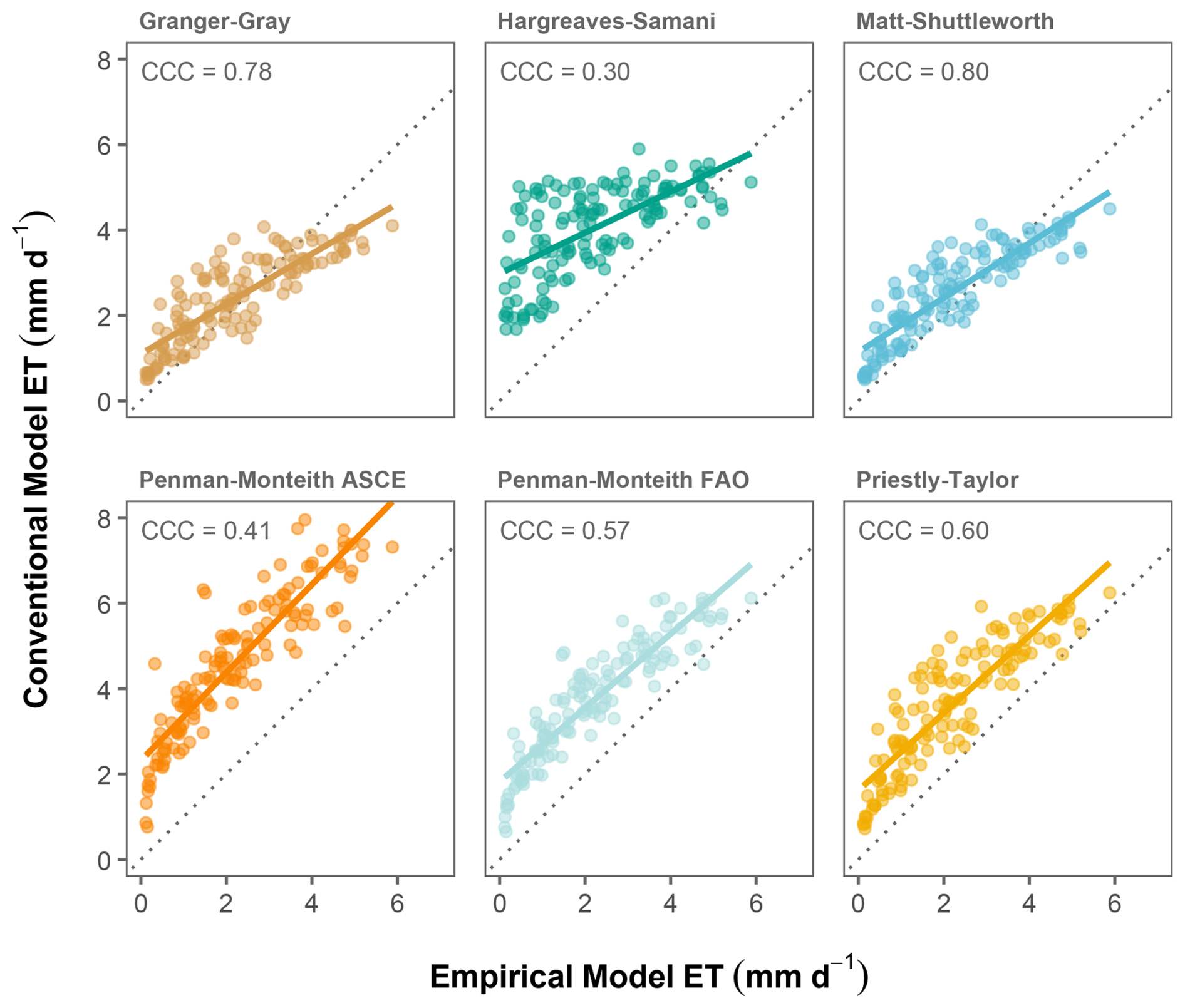
Figure 7 Daily ET calculated from our basin-scale, empirically-based model vs. ET from six conventional models. Dotted lines depict 1 : 1 relationships. CCC = concordance correlation coefficient.

Differences in conventional model assumptions and parameterizations likely explain their variable performance. The MS equation was developed for arid and semi-arid climates, and the GG model explicitly assumes non-saturated soil (McMahon et al., 2013), which may explain why they underestimated relatively high ET rates. Similarly, the relatively weak sensitivity of HS to atmospheric conditions may explain why it overestimated ET at lower rates but underestimated ET at higher rates. However, model parameters that more closely matched conditions in Basin A did not necessarily result in better performance. For example, the mean vegetation height in Basin A was 36 cm, yet PM-FAO, which assumes a 12 cm plant height, had better agreement than PM-ASCE, which assumes a 50 cm plant height.

The strong linear relationships between our empirical ET estimates and those from PM models likely reflect their shared sensitivity to the atmospheric variables that control ET, particularly solar radiation and vapor pressure deficit. However, the two approaches use very different methods to account for surface and aerodynamic factors. The empirical model was parameterized directly from measurements within Basin A and incorporated spatial variation in plant height, radiation, and topographic position explicitly, but other factors (like wind speed) implicitly. In contrast, the PM formulations account for vegetation and aerodynamic factors only via their inbuilt parameters but explicitly incorporate wind speed. Wind speed did appear to influence the discrepancy between PM and empirical ET estimates, as differences increased significantly with wind speed for both PM formulations (p < 0.001; Fig. S3). Further, while wind speed explained 39 % and 12 % of the variation in these differences for PM-ASCE and PM-FAO models, respectively, it explained ≤ 5 % for the other conventional models, suggesting that the treatment of wind speed contributed to PM estimates being greater than the empirical estimates. Although wind speed was not an explicit predictor in the empirical model, airflow generated by the chamber mixing fans influenced the measured fluxes and was therefore implicitly represented in model calibration. However, the magnitude of this influence is uncertain because wind speed within chambers was not measured. Moreover, wind speed data used in the PM models may not have fully represented conditions within the basin, since surrounding and internal structures could have reduced and/or accelerated airflow.

Further, soil-water limitation explained only a modest amount of the discrepancy between conventional and empirical ET estimates. Across the range of effective rooting depths we evaluated (20–40 cm), mean daily water-stress coefficients (K_S) ranged from 0.969 to 0.987, indicating that meaningful water limitation was infrequent during the model-comparison period. There were periods when K_S fell below 0.75, but these accounted for only 6 %, < 1 %, and 0 % of days when using 20, 30, and 40 cm rooting depths, respectively. Nonetheless, incorporating K_S reduced the overestimation by the PM models by 5 %–7 % (with a 30 cm rooting depth), primarily by decreasing ET at the upper end of its range, but it also reduced concordance between empirical ET and all six conventional models (Fig. S4). Thus, although not accounting for soil-water limitation contributed slightly to the higher ET estimates from the PM models, it is unlikely to explain their systematic offset from empirical ET. Other differences between the approaches, including their representation of vegetation characteristics and surface resistance, likely account for much of the remaining systematic offset.

Other researchers have similarly observed variability in the prediction capabilities of conventional ET models applied to bioretention basins. For example, PM-ASCE closely tracked measured ET in a mesocosm with unrestricted drainage but underestimated ET for a mesocosm with an internal water storage device (Hess et al., 2017). The PT model consistently underestimated ET in a bioretention mesocosm with mixed, short-stature vegetation (Wadzuk et al., 2015) and prairie plants (Nocco et al., 2016), whereas it was fairly accurate for experimental basins planted with shrubs or turfgrass (Nocco et al., 2016). Based on a review of these and other studies, Ebrahimian et al. (2019) recommend using the HS equation, arguing that, while it typically overestimates bioretention ET, this is outweighed by the fact that it only requires temperature and location data as inputs. Given that HS had the lowest CCC among the six models we evaluated, we recommend using other models if the required data are available, but we acknowledge that HS may be the only viable option if they are not.

3.6 Estimation using shade coefficients

Application of the shade coefficient to the input solar radiation data yielded improved agreement when using the PM-ASCE, PM-FAO, and PT models (CCC_shade= 0.44, 0.63, and 0.68, respectively) but made a negligible difference when using the other models (Fig. S5). This improvement was smaller than initially expected, likely because Basin A was oriented east-west, with the highway wall to the north, meaning the sun was less often blocked by the wall than it would be at many other sites. Given that the data needed to generate shade coefficients are frequently available (i.e., high-resolution DEM, software to model direct and diffuse radiation, and a solar radiation sensor in an unshaded location), we recommend that shade coefficients be determined and used in ET modeling whenever possible, especially for basins subject to shading from tall structures.

3.7 Estimation using landscape coefficients

The landscape coefficients (K_L) we calculated (approximately 0.5 to 1.0; Table 4) were in the range of K_L values previously determined for park-like landscapes with mixtures of plant types (Sun et al., 2012; Pannkuk et al., 2010; Nouri et al., 2013). Applying these K_L values to the ET estimates from the majority of conventional models (PM-ASCE, PM-FAO, PT, and HS) improved agreement with those from our empirically-based approach (Table 4; Fig. S6). A mathematical byproduct of applying multiplicative corrections when initial estimates were greater than ours is that it made conventional models less responsive to changing environmental conditions.

Table 4 Landscape coefficients (K_L), 95 % confidence intervals (CI), and concordance correlation coefficients (CCC) for the six conventional ET models. CCC were calculated in comparison to the whole-basin empirical model. Original = no adjustment to conventional model. Shade = model included shade coefficient adjusted solar radiation. K_L=  model correction based on landscape coefficient. Additive = model correction based on linear regression intercept. Numbers in bold highlight the highest concordance correlation coefficient for each model.

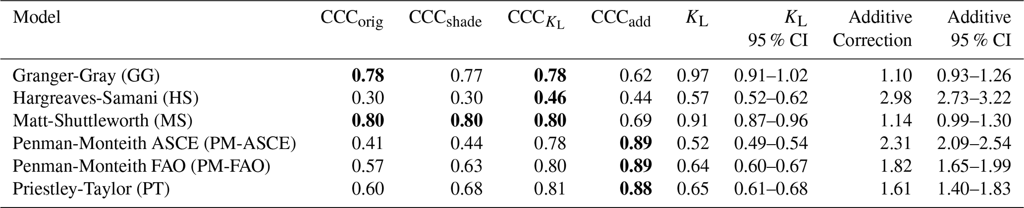
The K_L correction yielded the greatest improvement in agreement for HS estimations (CCC_KL= 0.46), though this model far underperformed all other models even with the correction. MS and GG stood out in having relatively large K_L (> 0.90), meaning corrections were smaller than for other models. The PM-ASCE-based K_L (0.52 ± 0.03) was slightly lower than the PM-FAO-based K_L (0.64 ± 0.03) (Table 4), corresponding to the greater plant height assumed by PM-ASCE (50 cm) vs. PM-FAO (12 cm).

The K_L approach to ET estimation is useful because it can be tailored to specific environments and conditions (e.g., Nouri et al., 2013). K_L values can be adjusted through the growing season to reflect shifts in plant size and the associated changes in the actual ET vs. ET₀ relationship through time (Pannkuk et al., 2010). However, the method may be difficult to apply to larger woody vegetation since the relationship between ET₀ and actual ET can be non-linear (Litvak et al., 2017). Nonetheless, our results indicate that K_L-based adjustments can provide reasonable estimates of actual ET in bioretention basins when used in basins with small- to medium-stature woody vegetation. This approach was particularly effective for models whose ET₀ estimates had approximately linear relationships with our empirically-determined ET values, such as PM-ASCE and PM-FAO.

3.8 Estimation using additive correction factors

Applying an additive correction factor substantially increased CCCs for three of the conventional models (PM-ASCE, PM-FAO, and PT), indicating that their corrected estimates (CCC_add= 0.89, 0.89, and 0.88, respectively; Fig. S7, Table 4) more closely matched our empirically-derived ET values than did the uncorrected estimates. Additive corrections were more effective than landscape coefficients since these three models systematically overpredicted ET relative to our empirical approach. However, additive correction also produced negative daily ET estimates when uncorrected values were small, highlighting a limitation of this approach. Nonetheless, for these three models, additive correction yielded the greatest agreement with our empirical estimates.

In contrast, additive corrections yielded poorer agreement with our estimates for the MS and GG models (CCC_add= 0.69 and 0.62, respectively). In fact, none of the correction methods we tried improved agreement for either of these models with the empirically-derived values. This may be because there was already relatively good agreement (CCC ≈ 0.8), potentially due to the fact that MS and GG incorporate soil moisture limitation. MS does so implicitly, since it is essentially a variant of the PM model tailored for (semi-)arid climates (Shuttleworth and Wallace, 2009). GG explicitly accounts for unsaturated soil conditions by including a coefficient for surface resistance into its estimation of ET (Granger and Gray, 1989).

3.9 Implications for bioretention design

The findings of this study have several implications for ET quantification and plant placement during the basin design process. Most importantly, several conventional ET models have the potential to accurately estimate ET in bioretention basins, despite their highly variable environments. Our findings therefore provide a potential means of improving the representation of ET in water balances used during basin design. For those with similar designs and in similar contexts to Basin A, the PM-ASCE, PM-FAO, or PT models could be used along with the correction factors we derived for Basin A, although the transferability of those corrections should be carefully evaluated. When the assumption of similarity to Basin A cannot be made, locally appropriate correction factors would need to be developed (McEvoy et al., 2022). One approach would be to develop locally appropriate K_L values through measurements of existing bioretention systems, with the resulting values applied to systems of the same type within a given region. Alternatively, K_L values could be estimated from species, vegetation density, and microclimate characteristics following the procedure outlined by Costello et al. (2000). The resulting ET estimates could improve predictions of stormwater volume reduction for proposed basins. Future measurement campaigns spanning a broader range of bioretention designs and environmental settings could establish the extent to which correction factors can be transferred among systems.

The HS model produced comparatively poor predictions for our basin. This model requires the least amount of climate input data since it estimates solar radiation based on latitude and time of year and makes assumptions about other meteorological variables (Guo et al., 2016). Considering the increasing availability of weather and solar radiation data, the simplifications of the HS model may become increasingly unnecessary. Instead, designers may be able to capitalize on other, more accurate models.

Additionally, our method of computing shade coefficients may be a simple yet useful means of adjusting solar radiation time series to increase the accuracy of ET estimates from conventional models, especially for sites with substantial shade from nearby infrastructure. The only requirements beyond a solar radiation time series are a high-resolution DEM of the site and software to compute direct and diffuse solar radiation from the DEM (such as ArcGIS).

Finally, engineers and landscape architects designing bioretention basins can potentially raise ET by placing plants that will grow larger (or otherwise produce greater leaf area) in appropriate locations within the basin. This might include basin flanks that receive little shade; locations that are frequently flooded may or may not be appropriate depending on the duration of soil saturation and soil salinity levels (Muerdter et al., 2018; Caplan et al., 2024). Larger plants may have utility in bioretention basins with internal water storage capacity (Hess et al., 2017). A potential tradeoff of increasing the size and extent of plants in a bioretention basin is the need to ensure access to adequate soil moisture through dry periods, especially since soil media is typically coarse-textured and can dry out substantially between rain events (Houdeshel et al., 2012; Nocco et al., 2016). This is a particular challenge in drier climates (Orr, 2013). We note that plants with deeper root systems (including large shrubs and trees) can access water over a broader depth range, lessening this limitation (Caplan et al., 2019).

3.10 Study limitations

Our empirical data came from a single bioretention basin, limiting the generalizability of our statistical model and basin-scale ET estimates. Nonetheless, the conclusions are likely applicable to other sites given that Basin A contains many design features common in bioretention basins. These include the structure (a central flow path flanked by sloped sides), partial shading from surrounding structures, taxa common in GSI in the Mid-Atlantic region (Myers et al., 2026), and sandy loam soils.

Second, ET estimates for the largest plants in the basin required extrapolation from measurements from only modestly large plants, since our flux chambers were ∼ 100 cm tall. Although plants taller than the chambers covered only ∼ 10 % of the basin area, they did have a disproportionally-large influence on basin-scale ET rates.

Third, although spatial variation in solar radiation was explicitly represented in our ET quantification, other microclimatic factors were assumed to be uniform. This is likely justified because air (and thus its temperature and humidity) tends to be well mixed at the basin scale, whereas solar radiation can be extremely variable over short distances due to shading. Nonetheless, VPD and wind speed could vary spatially within bioretention systems, particularly where surrounding structures and vegetation alter microclimate and airflow. Future studies could incorporate spatial measurements of these variables to determine whether accounting for this additional heterogeneity improves basin-scale ET estimates.

Finally, we could not calculate ET's contribution to stormwater volume reduction since we lack data on inflow into Basin A. Empirical measurement was attempted but unsuccessful. Direct measurement did not capture low flows and approximating it using precipitation records in combination with directly-connected impervious area (DCIA) was highly unreliable because DCIA appeared to change through time depending on highway construction activities and other factors.

4 Conclusions

Bioretention basins and other types of green stormwater infrastructure play an important role in offsetting the negative hydrologic impacts of impervious surfaces. To design these systems optimally, we need methods of accurately quantifying a basin's ability to reduce stormwater volume not only through infiltration but also through evapotranspiration (ET). However, ET involves multiple soil, plant, and meteorological processes, all of which are highly variable in space and time, and some of which are challenging to measure directly.

We parameterized a spatially-explicit ET model for a bioretention basin based on measurements of water flux from soil and plants, plant size, soil moisture, weather, and shade cast by nearby buildings and other structures. This empirical whole-basin model explained most of the observed variation in ET. The model was particularly sensitive to plant height and shade, both of which should be carefully measured or estimated when modeling bioretention basin ET. They are also factors that designers can influence, meaning that ET can likewise be moderated through design.

Quantifying ET at fine spatial scales is typically unnecessary for bioretention basin design or system evaluation. While instructive for elucidating sources of ET variation within a basin, directly measuring ET within bioretention basins is a laborious process requiring specialized equipment not commonly part of stormwater practitioners' toolkits. Penman-Monteith (both ASCE and FAO) and Priestley-Taylor models produced estimates that consistently overestimated ET in comparison to our empirical model. Depending on the accuracy required, these model estimates could be used without correction, with the understanding that they are likely to overestimate ET, or they could be adjusted using additive, multiplicative, or shade-based corrections to improve agreement with empirical ET. We note that additive correction is highly context-specific and may produce negative estimates at low ET rates and should therefore be used with caution. Matt-Shuttleworth and Granger-Gray also had good agreement with our empirical model, though they tended to underpredict high ET rates and overpredict low ET. The Hargreaves-Samani model had the poorest agreement regardless of correction factors used, likely because it only requires temperature data and estimates solar radiation based on location rather than measurements. When sufficient meteorological data are available, the Penman-Monteith and Priestley-Taylor models are particularly suitable for bioretention applications because they are sufficiently responsive to variation in atmospheric conditions and their systematic biases can be reduced or removed using locally appropriate corrections.