Undercatch corrected gridded precipitation data to improve hydrological modeling in high-alpine orography

Stationary precipitation measurements are frequently affected by undercatch errors, which are particularly pronounced in cold and alpine regions with strong winds. Since gridded precipitation products used in land surface modeling are often derived from spatial interpolation of meteorological station data, these measurement errors propagate directly into gridded datasets. In this study, we train monthly Generalized Additive Models (GAMs) using undercatch corrected station observations, with geographical exposure and terrain elevation as predictors, achieving R² values above 0.76 in Leave-One-Out Cross-Validation. We apply these models to generate monthly undercatch correction factors for Austria and – combined with an exposed terrain penalty – use them to adjust existing station-based gridded precipitation products. We validate the undercatch correction using the conceptual rainfall-runoff model COSERO across Austria and in two high-alpine reservoir catchments: Kölnbrein and Schlegeis. Our results demonstrate that retrospectively corrected precipitation reduces runoff simulation biases across Austria, especially in catchments above 1500 m elevation, and closes the water balance in both alpine study regions where uncorrected data showed runoff deficits exceeding 20 %. Biases in snow depth simulations – assessed using the physically-based snowpack model Alpine3D and validated against stereo-satellite observations – decrease from a median difference of −0.87 to +0.15 m. Additionally, undercatch-corrected precipitation enables more realistic simulations of snow covered area during the melting season and long-term glacier volume changes. The proposed method shows promising results in both alpine case study catchments and across Austria, highlighting the importance of accounting for undercatch errors in high-alpine terrain and indicating the need for further research into their magnitude at high elevations.

1 Introduction

Globally, precipitation measurements from gauging networks and their spatial interpolation provide essential data for water resource management, hydrological and climate modeling, flood forecasting, hydropower operations, agricultural planning, ecosystem assessments, and infrastructure design. In mountainous regions, steep slopes and complex terrain influence the spatial variability of precipitation (Gnann et al., 2025) and challenge measurement accuracy. Simultaneously, water resources management in these regions faces increasing pressure from climate change impacts on alpine temperatures, snow dynamics, and glacier mass balance (Ohmura, 2012; Zekollari et al., 2019). As global temperatures rise, reliable precipitation estimates become increasingly critical for predicting shifts in snow melt timing, changes in water availability (Ford et al., 2020), and impacts on hydropower generation in alpine regions (Wasti et al., 2022).

Stationary precipitation measurements are affected by undercatch, since airflow around the gauge and the instrument geometry itself deflect falling hydrometeors away from the inlet (Sevruk et al., 1991). The magnitude of this effect depends on wind speed (Kochendorfer et al., 2017b; Wolff et al., 2015), precipitation phase, size and density (Thériault et al., 2012; Judson and Doesken, 2000) – and thus temperature – as well as precipitation intensity (Colli et al., 2020), and gauge and shielding design (Colli et al., 2015). Atmospheric conditions in cold or high-alpine regions with complex orography produce particularly significant undercatch due to low temperatures and high wind speeds. The quantification of undercatch measurement errors and the derivation of suitable transfer functions to mitigate them have been extensively studied in various international meteorological field campaigns (Goodison et al., 1998; Smith et al., 2020; Kochendorfer et al., 2020). While transfer functions for undercatch correction have been developed and validated in various settings (Kochendorfer et al., 2017b, 2018), their applicability in high-alpine, complex terrain remains limited, since uncertainties in precipitation measurements are particularly pronounced and not all mechanisms are fully understood in complex orography (Kochendorfer et al., 2017a). This is reflected in the difficulty of reliably constraining high-elevation precipitation gradients, although additional data sources such as snow course measurements have been shown to substantially improve lapse-rate estimates (Avanzi et al., 2021). Furthermore, precipitation measurements in mountainous regions are often both quantitatively inaccurate and spatially unrepresentative (Bica et al., 2011; Lu et al., 2019; Weber et al., 2020; Gentilucci et al., 2021), with point-scale gauge observations often deviating significantly from actual areal precipitation (Bohnenstengel et al., 2011; Tang et al., 2018). These limitations are compounded by the fact that precipitation gauges in mountainous regions are predominantly installed at accessible valley floor locations, rather than at higher elevations with typically more severe undercatch effects (Ebert et al., 2007; Frei and Schär, 1998). Consequently, substantial precipitation adjustments are required in snow-dominated, wind-exposed regions, where undercatch-related uncertainties are greatest (Pierre et al., 2019).

Gridded precipitation products – like e.g. E-OBS (Cornes et al., 2018) or WorldClim 2 (Fick and Hijmans, 2017) – are frequently based on spatially interpolated or adjusted to meteorological station data, which suffer from the aforementioned undercatch errors in addition to other uncertainties caused by different databases and methods used to create the gridded products (Gampe and Ludwig, 2017; Filippucci et al., 2025). Some data sets address this problem by explicitly accounting for undercatch and representing complex terrain through model-based reference fields (Lussana et al., 2019), while others represent precipitation patterns through terrain-informed principal component approaches (Isotta et al., 2019). However, the ideal solution for tackling undercatch errors – generating gridded precipitation data using undercatch corrected stations – is not common practice. Consequently, the measurement errors at station level are propagated into these gridded datasets. Retrospectively correcting the gridded precipitation data with full accuracy would require perfect information about the atmospheric conditions at the station level and the interpolation process, which is typically neither available nor practical for users and impact scientists. The resulting biases in gridded precipitation products lead to systematic errors in water balance calculations, underestimation of water resources (Pulka et al., 2024; Immerzeel et al., 2015), and unreliable predictions of future water availability under climate change scenarios (Viviroli et al., 2011; Pepin et al., 2022), with direct consequences for hydropower planning, flood risk management, and ecosystem conservation. As biases increase with elevation and vary seasonally (Herrnegger et al., 2018; Henn et al., 2018), they pose a particular challenge for countries with high-alpine terrain and require retrospective correction after the gridded precipitation data have been created.

Several approaches have been developed to evaluate undercatch in gridded precipitation products. Independent in-situ precipitation measurements are used to assess biases (Rasmussen et al., 2012) and adjust spatial precipitation products (Livneh et al., 2014; Sun and Su, 2020; Schauwecker et al., 2021). While weather radars provide valuable information on the spatial structure of precipitation (Khanal et al., 2019), they are costly and have limited applicability in complex terrain due to ground clutter effects, observing geometry, and sub-grid-scale heterogeneity of precipitation systems (Goudenhoofdt and Delobbe, 2009; Kaltenboeck and Steinheimer, 2015; Barros and Arulraj, 2020). Furthermore, quantitative precipitation estimates from weather radars rely on calibration with ground-based gauge measurements, which in mountainous regions are subject to the aforementioned limitations of undercatch and lack of representative stations. Streamflow measurements can function as an indirect assessment for precipitation evaluation at the catchment scale when combining water balance modeling with evapotranspiration estimates (Kirchner, 2009; Herrnegger et al., 2015a; Immerzeel et al., 2015; Wortmann et al., 2018). In combination with snow-hydrological modeling, ground-based, airborne, and satellite remote sensing can provide insights into the spatio-temporal distribution of snow (Hedrick et al., 2018; Shaw et al., 2020; Yang et al., 2022; Alonso-González et al., 2023; Girotto et al., 2024; Premier et al., 2023; Ferrarin et al., 2025), thereby enabling quantitative estimates of solid precipitation distribution and undercatch errors (Vögeli et al., 2016; Pulka et al., 2024). Various approaches for correcting orographic precipitation effects across regional and global scales and for different hydrological processes have been proposed (Herrnegger et al., 2018; Lu et al., 2019; Adam et al., 2006). However, existing, widely used gridded precipitation products continue to require a systematic, transferable method for correcting regional errors in high-alpine terrain (Zandler et al., 2019).

Austria provides an ideal study region for investigating precipitation undercatch due to its complex alpine terrain, dense observational network, and high reliance on hydropower production. Hydropower accounts for more than 60 % of Austria’s domestically produced electricity (Urbantschitsch and Haber, 2024), making accurate precipitation estimates particularly important for water resources management and energy production (Wesemann et al., 2018). In high-alpine catchments, runoff is additionally influenced by glacier melt contributions (Koboltschnig and Schöner, 2011; Koch et al., 2011; Weber et al., 2010). Austria’s complex orography, combined with a dense network of stationary precipitation measurements (Fig. 1a), enables the evaluation of precipitation undercatch across a wide range of elevation bands. The terrain spans elevations from approximately 115 to 3800 m a.s.l., resulting in pronounced gradients in precipitation, hydrological processes, and discharge regimes. In higher-elevation catchments, where precipitation rates exceed evapotranspiration (Gnann et al., 2025), hydrology is strongly controlled by snow accumulation and melt processes, both of which exhibit marked seasonal variability (Kling et al., 2006). These characteristics allow for a systematic assessment of precipitation undercatch across diverse elevations, exposure conditions, and hydrological regimes.

In this study, we apply a precipitation undercatch correction developed at the weather station scale (Kochendorfer et al., 2017a) to gridded precipitation data to generate a retrospective, gridded undercatch correction method for Austria. We quantify monthly undercatch correction factors at 261 individual weather stations using transfer functions from Kochendorfer et al. (2017a) and train Generalized Additive Models (GAMs) to spatially extend these corrections across Austria using geographical exposure and terrain elevation as predictors. The resulting correction factors are subsequently applied to the gridded precipitation dataset SPARTACUS (Hiebl and Frei, 2018). We further introduce an additional exposure-dependent penalty to account for remaining uncertainties in highly exposed terrain, stemming from different sources like the use of the undercatch transfer function in complex orography (Kochendorfer et al., 2017a), totalizers in the gridded base precipitation data (Hiebl and Frei, 2018) and potential plateauing of precipitation lapse rates through flow blocking and moisture depletion (Jiang, 2003; Houze, 2012; Gnann et al., 2025). The performance of the undercatch-corrected precipitation is first evaluated through runoff simulations in selected Austrian catchments using the conceptual rainfall–runoff model COSERO (Herrnegger et al., 2015b). Further validation is carried out in two high-alpine reservoir catchments (Kölnbrein and Schlegeis) using both COSERO and the physically based snowpack model Alpine3D (Lehning et al., 2006). Model results are compared against observations and/or reference data of runoff, glacier volume change, snow depth, and the evolution of the snow covered area in the melting period. This multi-model, multi-variable evaluation across different spatial scales enables a comprehensive assessment of the proposed undercatch correction method and provides insights into its robustness and remaining sources of uncertainty.

The results of this interdisciplinary study provide three key contributions: (1) publicly available monthly undercatch factors and associated metadata for 261 stations in Austria, (2) publicly available maps of undercatch correction factors for Austria at a 1 km resolution, both available under Maier et al. (2025), and (3) a validated approach for improving precipitation estimates and mitigating undercatch errors, evaluated with a conceptual hydrological and a physically-based snowpack model across Austria and two high-alpine study regions. We propose that the methods and results are transferable to other mountainous regions with similar characteristics and can directly support water resources management, hydropower operations, and climate change impact assessments in alpine environments.

2 Data and methods

2.1 Study Region

The study region comprises Austria and adjacent headwater catchments, as depicted in Fig. 1a. Approximately 60 % of Austria's national territory is covered by the Alps, a region that is particularly sensitive to climate change (Haeberli and Beniston, 1998; Viviroli et al., 2011; Matiu et al., 2021). Austria's geography and climate are therefore strongly shaped by its complex orography, with the Alps covering the west and south and the comparatively drier and flatter alpine forelands and lowlands in the north and east. Due to its central European location, the Austrian climate is influenced by both the Atlantic and the Mediterranean, while also exhibiting continental climatic influences (Bozzoli et al., 2024).

In addition to modeling the whole of Austria, two high-alpine study regions were selected to validate the precipitation correction at high elevations: the reservoir catchments of Kölnbrein (50 km²; Fig. 1b) and Schlegeis (110 km²; Fig. 1c). Both are partially glaciated (11 % for Kölnbrein and 22 % for Schlegeis in 2003 (RGI Consortium, 2017)) and have similar mean elevations (2430 m for Kölnbrein and 2540 m for Schlegeis). Despite these similarities, the two regions are subject to different atmospheric conditions: Schlegeis is located north of the Alpine main ridge and is predominantly influenced by the Atlantic, whereas Kölnbrein lies south of the Alpine main ridge and is more strongly affected by Mediterranean conditions (Bozzoli et al., 2024).

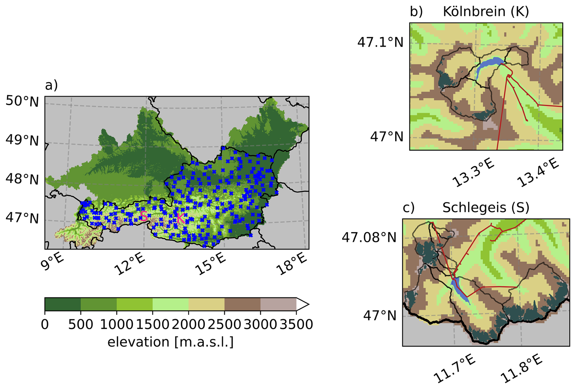
Figure 1 Topography of (a) Austria and adjacent headwater catchments of the Inn, Rhine, Danube and Morava, and the high-alpine reservoir catchments (b) Kölnbrein (K) and (c) Schlegeis (S) in m a.s.l. The blue crosses in panel (a) mark the weather stations used to derive the undercatch functions. “S” and “K” mark the location of the two study regions. In panels (b) and (c) hydrological subcatchments are shown in black lines, glaciated areas in gray, reservoirs in blue and waterlines in red. The thick black line in panel (c) displays Austria's border.

2.2 Weather Station Data

This study utilized 10 min measurements of temperature, wind speed, and precipitation from semi-automated weather stations, provided by GeoSphere Austria, Austria's federal institute for geology, geophysics, climatology, and meteorology (GeoSphere Austria, 2024). All meteorological variables required in this study are recorded automatically, while some (unused) parametrizations like cloud type, as well as downstream quality control are performed by experts. Precipitation is predominantly measured using tipping-bucket gauges, although the number of weighing gauges has increased in recent years (Haslinger et al., 2025). To ensure data quality, stations were required to provide at least ten years of measurement records for every month and to exhibit plausible average precipitation values. Stations were not required to cover a common overlapping period, which reduces the influence of decadal variability on the derived correction factors; the full period from which station data were drawn is 1995–2024. The stations are densely distributed across Austria, as shown in Fig. 1a. Austria's two highest stations, located at elevations of 2864 and 3109 m, were excluded from the station ensemble since they would otherwise place disproportionate weight on elevation bands with low station density. This process resulted in a final set of 261 stations, with the highest remaining station at 2327 m and the majority of stations being located below 1500 m (see Fig. 7 for the elevation distribution). As the catch efficiency transfer function utilized in this study (Kochendorfer et al., 2017a) was derived using 30 min measurements, the 10 min data were aggregated to 30 min temporal means for wind speed and temperature and 30 min sums for precipitation.

2.3 Historical Climate Data

Temperature and precipitation data were assembled from multiple pre-existing gridded climate products, prepared by Lehner et al. (2025), as described in more detail below. For Austria and the Swiss Engadin, the GeoSphere Austria SPARTACUS dataset was used (Hiebl and Frei, 2016, 2018). SPARTACUS provides daily meteorological information intended for climatological applications. The station observations incorporated in this data set originate from long-term, homogenized weather stations in and around Austria, including totalizers in some high-alpine regions to reduce measurement errors (Hiebl and Frei, 2018). Consequently, the stations used in this study for undercatch correction only partly overlap with those included in the gridded data set. For the neighboring regions of the Bavarian Danube and Czech CHELSA (Karger et al., 2023) and WorldClim 2 (Fick and Hijmans, 2017) were used. We smoothed the transitions between the data sets using a 10 km feather-blending zone. The resulting data set consists of daily values for the period 1961–2023 with a spatial resolution of 1 km. The geographical predictors used in GAM training were derived from the same topographic data used in the SPARTACUS product. After applying the undercatch correction in this study, both the raw and corrected precipitation data were patch-interpolated (Zhuang et al., 2025) to the study regions, which is an artifact-reducing, smoother, higher-order regridding method compared to bilinear interpolation. For the two study regions Kölnbrein and Schlegeis, additional meteorological variables at 250 m spatial resolution – originating from different data sets – were required to run the snowpack model Alpine3D (Lehning et al., 2006). Global radiation data was obtained from the GeoSphere Austria APOLIS product (GeoSphere Austria, 2013) and is crucial for accurately representing snow hydrological processes (Weber et al., 2021). Relative humidity was derived from downscaled SPARTACUS temperature and a station-based dew-point interpolation (Lehner et al., 2024). Wind speed was estimated using a station-based Ridge regression (Klisho et al., 2024). Potential evapotranspiration was calculated using the Penman-Monteith equation (Allen, 2000). Because wind directions are not realistic at 250 m resolution in complex terrain, dummy wind directions were calculated in this study. These consist of average hourly wind directions for precipitation and non-precipitation days, respectively, derived from the INCA dataset (Haiden et al., 2011). Further, all six meteorological variables – along with the patch-interpolated precipitation – were temporally disaggregated to hourly time steps within the two high-alpine study regions. Temporal disaggregation followed methods from Förster et al. (2016) and statistical approaches that relate daily means to hourly patterns from the ERA5 (Hersbach et al., 2020) or INCA dataset (Haiden et al., 2011), as documented in Formayer et al. (2023).

2.4 Undercatch Transfer Function

The catch efficiency CE transfer function used in this study is defined as

$$\begin{array}{}\text{(1)}& \mathrm{CE}=e^{-aU(\mathrm{1}-{\tan }^{-\mathrm{1}}(bT)+c)},\end{array}$$

with the constants a=0.0623, b=0.776 and c=0.431. U denotes the 10 m-wind-speed in m s⁻¹, capped at a maximum threshold of $U_{\mathrm{threshold}}=\mathrm{9}\mathrm{m}{\mathrm{s}}^{-\mathrm{1}}$ and T denotes the air temperature in °C (Kochendorfer et al., 2017a). This transfer function was developed for unshielded weighing gauges using wind speed measurements at 10 m mast height. Although tipping buckets are still the predominant gauge type in the GeoSphere Austria network, weighing gauges have been increasingly installed since the early 2000s (Haslinger et al., 2025). A similar transfer function for tipping buckets was proposed by Kochendorfer et al. (2020); however, we use the weighing-gauge formulation for our high-alpine application. This choice is motivated by the absence of an explicit temperature term in the tipping-bucket function and by its comparatively strong wind-speed correction, including corrections of around 30 % for T<2 °C and $U=\mathrm{0}\mathrm{m}{\mathrm{s}}^{-\mathrm{1}}$, which would have been difficult to implement in high-alpine regions as wind speeds are typically considerably higher at peaks (Graf et al., 2019). Figure 2 shows the CE as a function of wind speed for different temperatures. It highlights that CE exhibits an approximately linear behavior at temperatures above the freezing point, while temperatures below freezing lead to increasingly non-linear behavior (Kochendorfer et al., 2017a). Under pronounced cold and windy conditions, CE can drop to as low as 20 %. The corrected precipitation is calculated as

$$\begin{array}{}\text{(2)}& {\mathrm{pr}}_{\mathrm{corr}}={\displaystyle \frac{\mathrm{pr}}{\mathrm{CE}}},\end{array}$$

and subsequently aggregated to monthly values. Monthly correction factors are then obtained by relating pr_corr to the uncorrected precipitation pr, resulting in one climatological correction factor per station and month. While this aggregation leads to some loss of information and may oversimplify individual events, it does not introduce a systematic bias for climatological time frames, which are the focus of this study (see Fig. S1 in the Supplement) and is easily transferable for future studies. These station-based factors subsequently served as target variables in the GAM training.

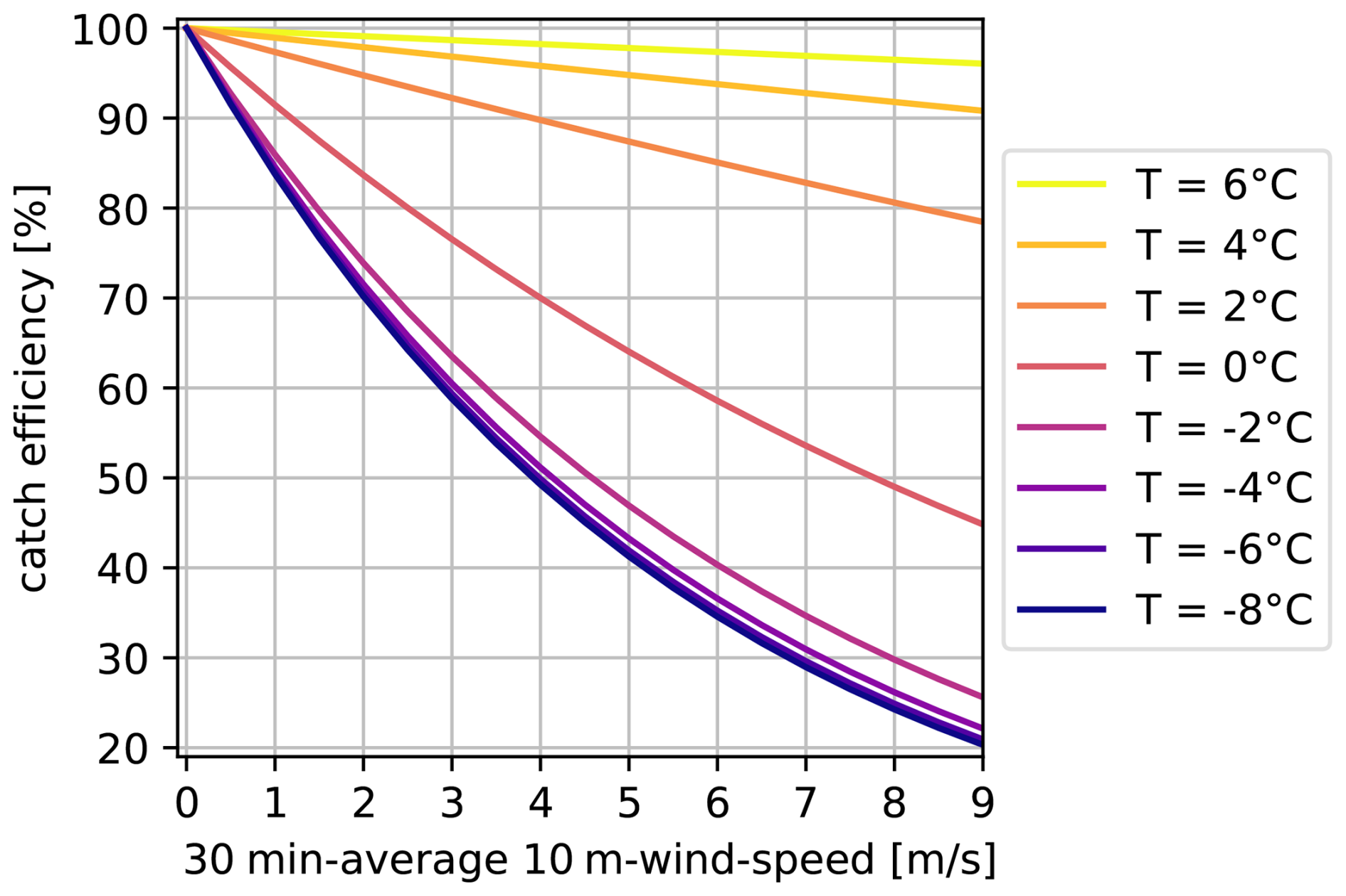
Figure 2 Catch efficiency in percent as a function of temperature and 10m-wind-speed as suggested by Kochendorfer et al. (2017a).

2.5 GAM Training

A comprehensive overview of Generalized Additive Models (GAMs) can be found in Wood (2017); with the key elements briefly recited here. A GAM is a generalized linear model that predicts the response variable y as a sum of smooth functions of predictor variables x_p, constructed using N splines of the form

$$\begin{array}{}\text{(3)}& f\left(\mathit{x}\right)=\mathrm{\Phi }\left(\sum _{p=\mathrm{1}}^N{\mathit{\varphi }}_p\left(x_{\mathrm{p}}\right)\right),\end{array}$$

with a monotonic function Φ. Under the assumption that the response variable follows a distribution from the exponential family E (e.g. normal or Poisson), it is linked to the smooth functions with a link function g as

$$\begin{array}{}\text{(4)}& g\left(E\right(y\left)\right)={\mathit{\theta }}_{\mathrm{0}}+f_{\mathrm{1}}\left(x_{\mathrm{1}}\right)+f_{\mathrm{2}}\left(x_{\mathrm{2}}\right)+\mathrm{\dots }+f_m\left(x_m\right),\end{array}$$

where θ₀ is the intercept and f_i are the smooth functions of the m predictors x_i. The smooth functions are then fitted so that a measurement of error (e.g. the Akaike information criterion (AIC) or the R² value) is minimized. To control model complexity and prevent over-fitting, an additional smoothness parameter λ is introduced, which penalizes smooth functions with high curvature (“wiggliness”). GAMs were chosen over potentially higher-performing machine learning techniques (e.g., random forests) because they allow for better and more direct physical understanding of the underlying process. Although constraining the maximum number of splines N and minimum smoothness parameter λ may reduce predictive power, the resulting smoother curves with low curvature further improved interpretability.

In this study, the response variable y – the station-based monthly undercatch factors – were approximately normally distributed after subtracting 1 and applying a logarithmic link function g=log. The predictor selection was based on concurvity analysis (Kovács, 2024), utilizing a HSIC-Lasso algorithm (Yamada et al., 2014; Climente-González et al., 2019), and an untuned random forest model (Breiman, 2001). The complete pool of possible geographical predictors is given in Sect. S2 in the Supplement. Both the HSIC-Lasso algorithm and the random forest model indicated high correlation between the geographical predictors, allowing the number of predictors to be significantly reduced.

The following three predictors x_i were identified as the most influential:

• terrain elevation, serving as a proxy for temperature, wind speed and precipitation amount,

• exposure (defined as the difference of topography on a 1 km grid to a smoothed topography) based on a 5 km smoothed topography, as a proxy for local climatological conditions and orographic complexity, and

• exposure based on a 51 km smoothed topography, as a proxy for synoptic wind exposure.

A graphical representation of these three predictors is provided in Sect. S3.

For each month, the optimal GAM configuration was determined by performing a hyperparameter grid search over the number of splines N and the smoothing parameter λ, evaluated using a Leave-One-Out Cross-Validation (LOOCV) across the 261 stations. Model performance was assessed using the mean R² value, with stations above and below 1200 m elevation given equal total weight to improve performance in higher elevations. The model configuration with the highest weighted R² value was selected for each month and subsequently applied to the gridded geographical predictors. Predictor values were capped at the minimum and maximum values observed in the training data to avoid extrapolation beyond the calibrated range.

2.6 Exposed Terrain Penalty

To mitigate the known uncertainties of undercatch transfer functions in complex terrain (Kochendorfer et al., 2017a, 2018), undercatch corrected precipitation in alpine regions was evaluated iteratively using catchment-scale hydrological observations for validation. Initial iterations revealed that, even with suitable GAM training scores, undercatch was substantially overestimated in high-alpine terrain and at exposed peaks. To address this, the maximum GAM-predicted monthly undercatch factor was capped at the maximum observed monthly station factor. Further, an exposed terrain penalty of the form

$$\begin{array}{}\text{(5)}& \mathrm{ETP}=\left(\mathrm{1}-\mathit{\alpha }\cdot {\displaystyle \frac{{\mathrm{EX}}_{\mathrm{51},>\mathrm{0}}}{max\left({\mathrm{EX}}_{\mathrm{51},>\mathrm{0}}\right)}}\right),\end{array}$$

was introduced. ${\mathrm{EX}}_{\mathrm{51},>\mathrm{0}}$ denotes the normalized, non-negative exposure derived from a 51 km smoothed topography. The penalty reduces pr_corr in mountainous regions, with a lower bound equal to the uncorrected precipitation pr. The penalty strength $\mathit{\alpha }=\mathrm{2}/\mathrm{3}$ was iteratively determined using hydrological modeling. The ETP aims to (1) reduce the overestimation of the undercatch magnitude in high-alpine terrain (Kochendorfer et al., 2017a, 2018), (2) account for the use of gauge totalizators in the gridded precipitation data set (Hiebl and Frei, 2018), which generally exhibit lower measurement errors, and (3) accounts for potential plateauing of precipitation lapse rates near high ridges, where flow blocking and moisture depletion can reduce orographic enhancement (Jiang, 2003; Gnann et al., 2025). Figure 3 displays the resulting ETP, showing the strongest reductions along the Alpine main ridge and for isolated high-elevation peaks.

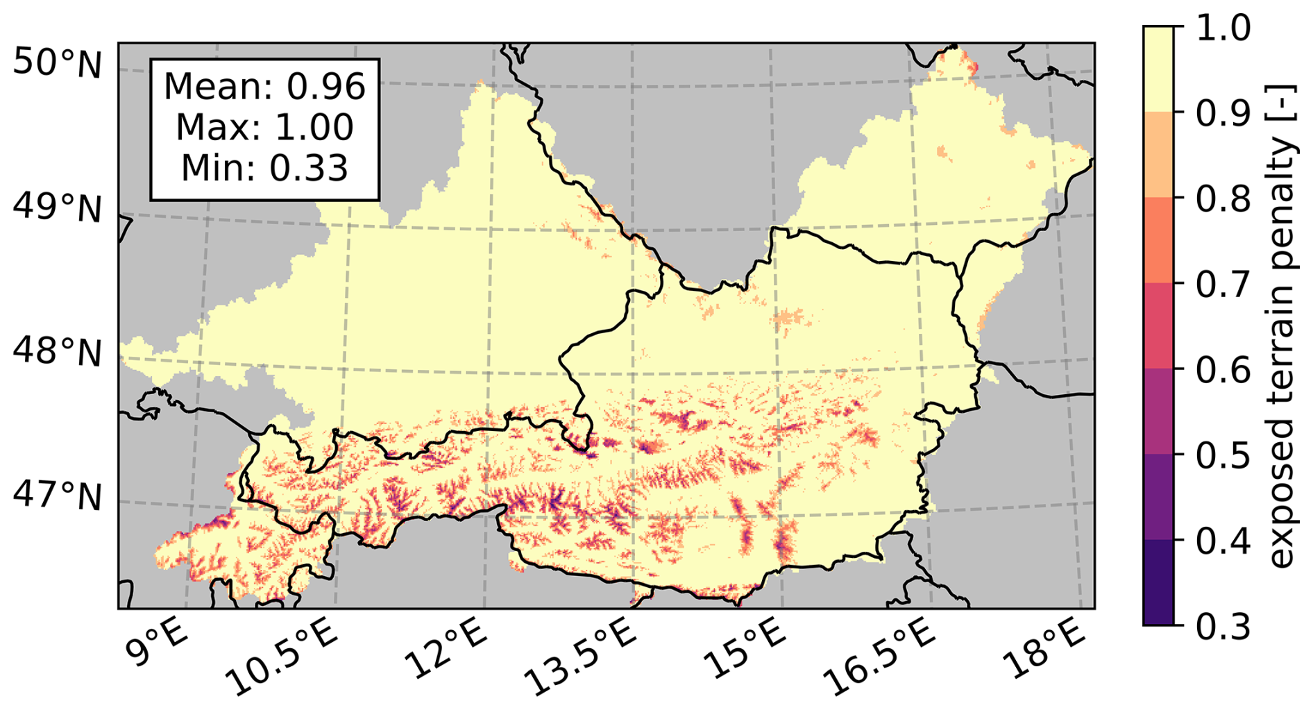
Figure 3 Color-coded exposed terrain penalty ETP for the full domain. Maximum, mean and minimum values are given in the text box.

2.7 Setup of Hydrological and Snowpack Models

Two models were used to validate the undercatch corrected precipitation data: the conceptual, semi-distributed rainfall-runoff model COSERO (Herrnegger et al., 2015b) and the physically-based, spatially distributed snowpack model Alpine3D (Lehning et al., 2006).

COSERO was used to validate the overall water balance in both the case study regions and across Austria. It is a HBV-style model (Bergström, 1992) that has been widely applied in hydrological and climate change impact studies across a range of spatial scales (Nachtnebel et al., 1993; Stanzel and Kling, 2018; Wesemann et al., 2018; Zeitfogel et al., 2025). All major runoff processes – including snow and glacier melt, evapotranspiration, and runoff routing – are simulated at the subcatchment scale, at an hourly resolution in the case study regions and a daily resolution for the whole of Austria. A schematic overview of the model structure is shown in Fig. 4. For the case-study basins, COSERO was set up with a spatial resolution of 100 m in glaciated areas and 250 m resolution in the remaining area. The Austrian-wide model was spatially discretized on a 1 km grid. The COSERO model domain includes some outlying headwater catchments, such as the Upper Inn in Switzerland (see Fig. 15). Due to computational constraints, the Upper Danube, Morava, and Inn in Germany were not modeled explicitly. Instead, observed runoff at the corresponding gauging stations was added to the model to close the water balance (see Qaddinflow in Fig. 4). Model calibration was performed against observed runoff using the Shuffled Complex Evolution algorithm (Duan et al., 1992, 1993) and the logarithmic Nash-Sutcliffe Efficiency (Nash and Sutcliffe, 1970) as the objective function. All basins were calibrated simultaneously to ensure seamless and spatially consistent parameter fields, with equal weighting in the objective function. Details on the initial parameter field for Austria can be found in Zeitfogel et al. (2025). The case study basins used the same initial information, except for a finer digital elevation model (DEM) with a 10 m resolution (Geoland.at, 2021). Calibration periods were 2015–2022 for the Kölnbrein catchment, 2012–2022 for the Schlegeis catchment, and 2001–2020 for the Austrian-wide model. The Austrian-wide model was independently validated for the period 1980–2000. For the two high-alpine case study regions, the full available observed runoff time series was used for calibration; therefore, no separate validation period was defined. In the Austrian-wide model, only a subset of catchments with low to medium anthropogenic influence (see Klingler et al., 2021, for definition) was included in the model calibration. An overview of all catchments, the calibration subset, added fluxes, gauging station information, and initial parameter fields can be found for the Austrian-wide model in Zeitfogel et al. (2025). Freely available discharge data from the Austrian Federal Ministry of Agriculture and Forestry, Climate- and Environmental Protection, Regions and Water Management (BMLUK, 2025), as well as time series from the LamaH dataset (Klingler et al., 2021), were used for model calibration in Austria. Reservoir inflow data for the Kölnbrein and Schlegeis catchments were provided by the Verbund Energy4Business GmbH.

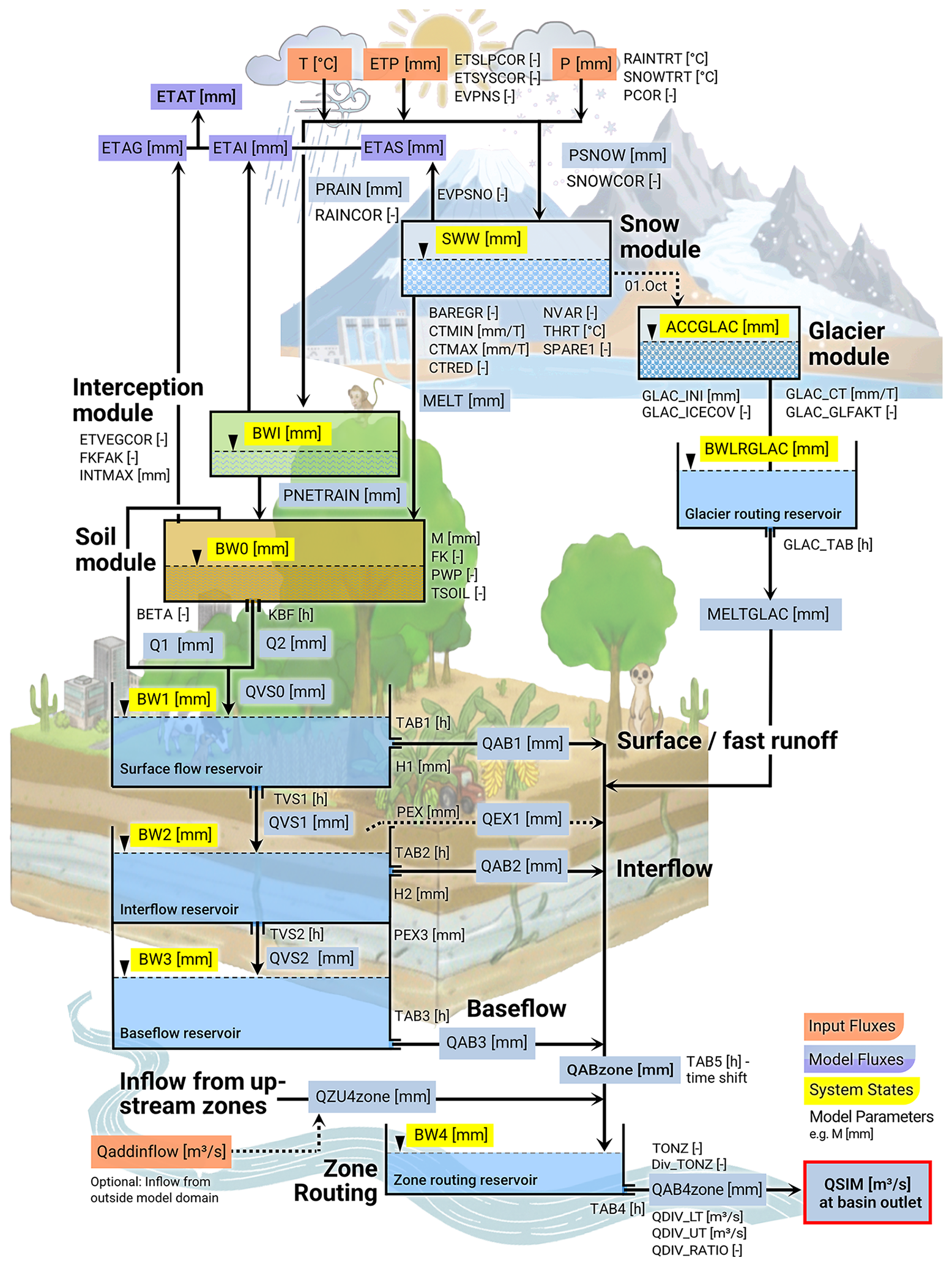
Figure 4 Schematic overview of the rainfall-runoff model COSERO, including model parameters, system states and fluxes (adapted from: Herrnegger et al., 2015b).

Alpine3D was used to indirectly validate solid precipitation amounts in the two high-alpine case study regions by (1) comparing the modeled snow depth to satellite observations, (2) comparing the snow covered area (SCA) to satellite observations, and (3) evaluating glacier volume changes against data from Hugonnet et al. (2021). The model setup required hourly meteorological input data for precipitation, air temperature, relative air humidity, incoming solar radiation, wind speed and wind direction following the settings presented in Koch et al. (2024). The same DEM and land cover information as in the COSERO setup were used. Glacier grid cells were initialized using glacier area and height maps from the Randolph Glacier Inventory (RGI) 2003 (RGI Consortium, 2017). Alpine3D was run at an hourly resolution, with a spatial resolution of 100 m for the smaller Kölnbrein catchment and 250 m for the larger Schlegeis catchment. Snowfall redistribution in Alpine3D was based on snow depth patterns derived from a WorldView-2 stereo satellite image. This map was provided by the VERBUND Energy4Business GmbH and was generated by subtracting the snow-on DEM stereo-satellite image, taken on 10 May 2021, from a snow-free airborne LiDAR DEM (taken in September 2020). The glaciated areas were omitted in the snow depth map to avoid potential offsets in snow depth due to glacier melt between autumn 2020 and spring 2021. Previous studies have shown that snow distribution patterns are generally consistent between years (Pflug and Lundquist, 2020; Bührle et al., 2023) and can therefore be inferred from a single satellite image taken close to the timing of peak snow water equivalent (Vögeli et al., 2016). To evaluate the SCA exemplarily during the snow melt period of 2021 in the Kölnbrein catchment, Sentinel-2-derived SCA (Gascoin et al., 2019) were used for all cloud-free observations (cloud cover <5 %) between May and July. Finally, modeled glacier volume changes were compared to global estimates of glacier volume change between 2000 and 2019 derived from satellite observations (Hugonnet et al., 2021), providing an additional, indirect constraint on simulated solid precipitation amounts.

3 Results and Discussion

3.1 Undercatch Factors

Figure 5a shows the monthly undercatch factors derived for wind, temperature, and precipitation station data as a function of station elevation, revealing a pronounced seasonal dependence of precipitation undercatch. The highest undercatch factors occur in winter, with a maximum in January, as shown spatially in Fig. 5b. Between May and September, all undercatch factors remain below 2.0, with minima in July and August, when factors are generally close to 1. While not all high-elevation stations show strong undercatch – indicated by the color-coding of the data points – all undercatch factors exceeding 2.5 are associated with stations with an elevation above 1300 m. These undercatch factors, along with associated station meta data, are publicly available (Maier et al., 2025).

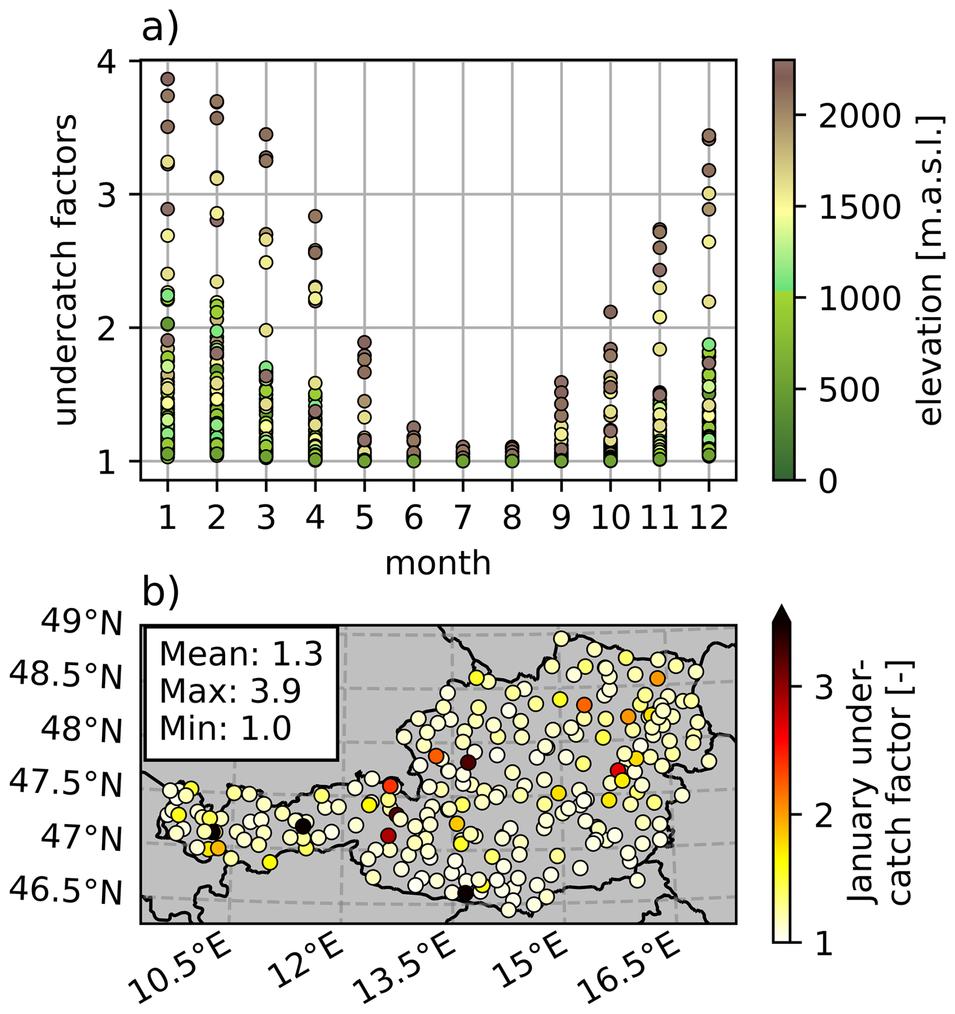
Figure 5 (a) Station-derived monthly undercatch factors. The color-coding refers to the station elevation of the data entries in [m a.s.l.], where green colors show stations with low and brown and yellow colors stations with high elevation. (b) Spatial distribution of January undercatch factors (color-coded) across Austria.

The undercatch factors in Fig. 5a increase with elevation as expected, reflecting the typical increase in wind speed and decrease in temperature with elevation, as well as the increased fraction of solid precipitation during winter months. As elevation is the dominant influence, temperature appears to be the main driver of undercatch. Further, as Fig. 5b suggests, no clear spatial structure is apparent in the undercatch factor distribution besides the tendency of increasing undercatch towards Austria's west, where highly-elevated stations are located.

Despite extensive quality control of the 261 stations, residual uncertainty is expected at high-alpine sites. This uncertainty could arise from local installation constraints, where precipitation gauges and wind sensors are not always co-located. Nevertheless, the station-based undercatch analysis yields physically plausible results, justifying the use of the derived undercatch factors as target variables for GAM training.

3.2 GAM Smooth Functions and Scores

The results of the monthly GAM hyperparameter grid search with LOOCV, with an emphasis on interpretability over maximum predictive performance, are summarized in Table 1. The first column shows the month corresponding to the undercatch factors used for the GAM training. The second column shows the weighted R² value of the LOOCV, where stations above and below 1200 m were assigned equal total weight. The average R² value across all months is 0.826, with the lowest performance in January (0.769) and the highest in May (0.904). The third and fourth columns show the selected hyperparameters, namely the smoothing parameter λ and the number of splines N. The models tend to select either high λ combined with small N, resulting in very smooth response functions, or the opposite configuration, allowing increased curvature. This behavior is also visible in Fig. 6. Overall, the winter half-year tends to have smoother curves, which indicates more explainable behavior in colder conditions. A comparison of the maximum predicted factors (y_pred,max; fifth column) and the true maximum station-based factors (y_true,max; last column) indicates a tendency towards overestimation during the winter half-year and slight underestimations during summer. Since the application of GAM-derived factors on the gridded data set is capped at y_true,max, the overestimation in winter has a limited impact on the final gridded results. Higher uncertainty at highly exposed stations can also be seen in the individual GAM plots provided in Sect. S4. Figure 6 presents all twelve smooth functions from the individually trained GAMs. The curves show the exponentially back-transformed relationships between the undercatch factors and the individual predictors, with the undercatch factor calculated as the product of the individual spline values. Terrain elevation (Fig. 6a) emerges as the dominant predictor, with contributions that can exceed those of the two exposure metrics (Fig. 6b, c) by up to one order of magnitude, particularly in summer at higher elevations. Although this may appear counterintuitive, the pronounced seasonal dependence of the intercept factor in Fig. 6d is key to understanding this behavior. The large summer values in panel (a) are multiplied with intercept factors close to zero in panel (d). Thus, the steep slopes of the elevation functions are required to accurately represent the onset of snowlines, while still predicting undercatch factors at the highest peaks. Since undercatch is generally more pronounced in winter, this behavior is not suggested by the GAMs during the winter months, when the smooth function contributions are multiplied by a larger intercept factor. The exposure predictors (Fig. 6b, c) tend to capture finer-scale behavior and are characterized by stronger curvature. In Fig. 6b, the particularly strong response in March (purple) is notable and is likely attributable to concurvity among the predictors: the simultaneous decrease of both 51 km exposure and elevation contributions in that month is compensated by a strong increase in the 5 km exposure smooth function. We therefore interpret this feature as a model artifact. In Fig. 6c, a clear seasonal distinction is visible: winter months show increasing undercatch with positive exposure values, whereas this response saturates or even reverses in summer, when the steep elevation smooth functions dominate the correlation at high elevations.

Table 1 Monthly GAM LOOCV hyperparameter grid search results and maximum predictions.

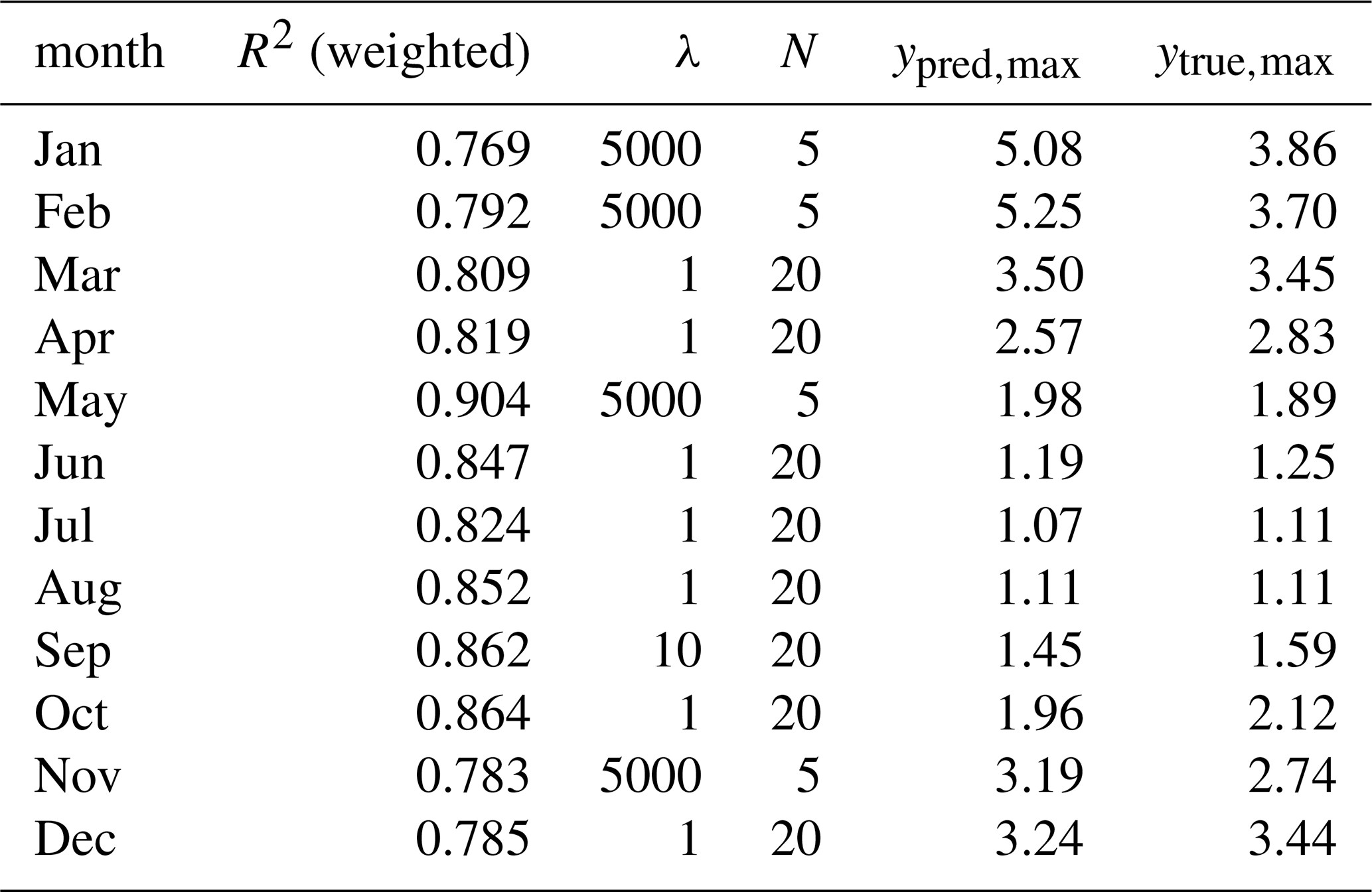
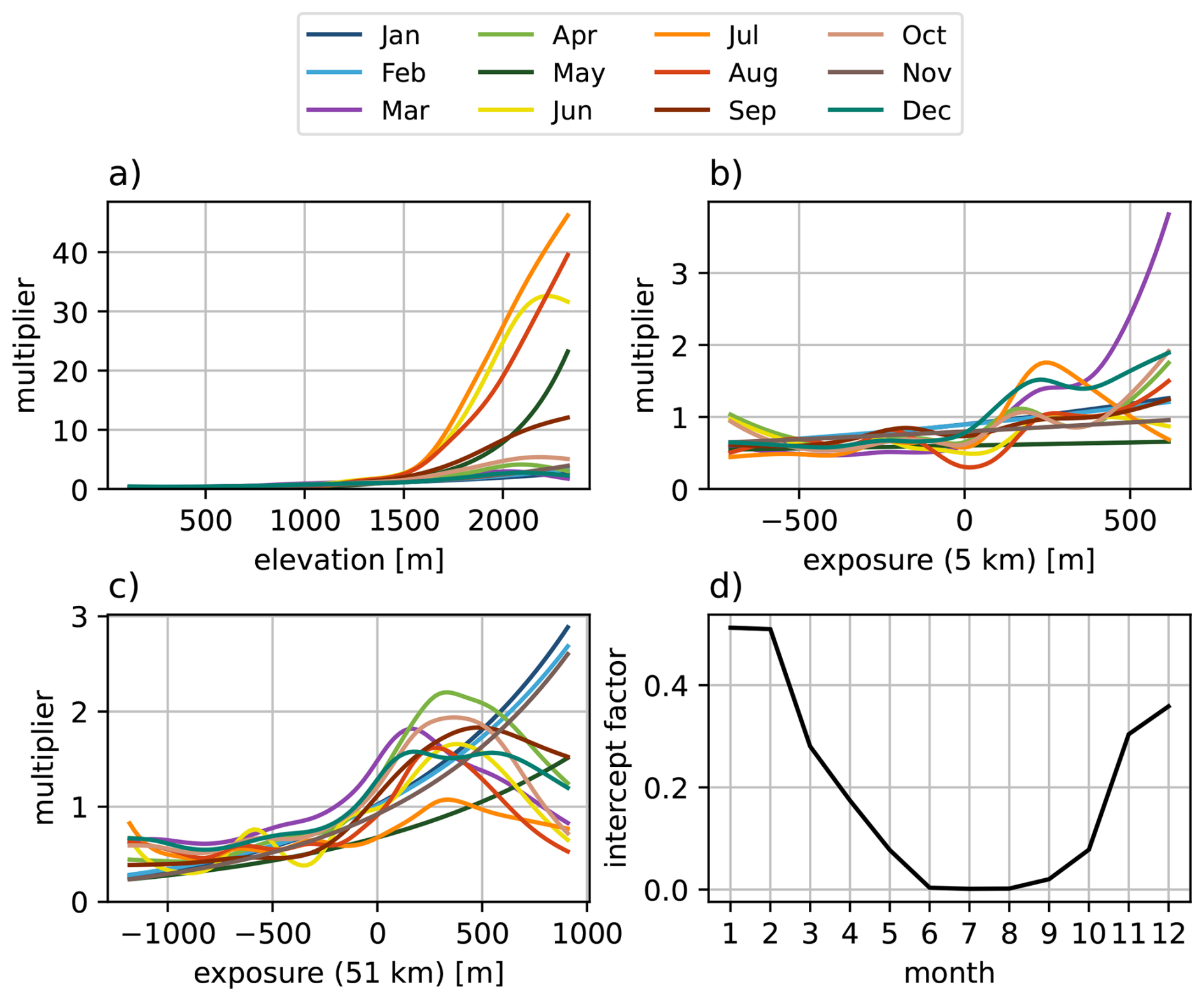
Figure 6 GAM smooth functions, color-coded for every month. Panels (a)–(c) show the back-transformed multiplier to the undercatch factors, dependent on the three selected geographical features elevation, exposure (5 km) and exposure (51 km). Panel (d) shows the constant intercept, which varies per month.

Figure 7 shows the relative monthly GAM error, averaged over all months for each station. The error generally increases with elevation (with a Pearson correlation coefficient of 0.61), following undercatch transfer-function uncertainty inferred from colder temperatures and higher wind speeds (Pierre et al., 2019; Kochendorfer et al., 2017a). The relative error for the 18 stations above 1500 m averages to 0.15 as compared to the average error of 0.02 for the stations below this elevation. The highest relative errors tend to occur at stations with positive exposure values, as indicated by the colorbar, which is also visible in the individual GAM smooth functions in Sect. S4.

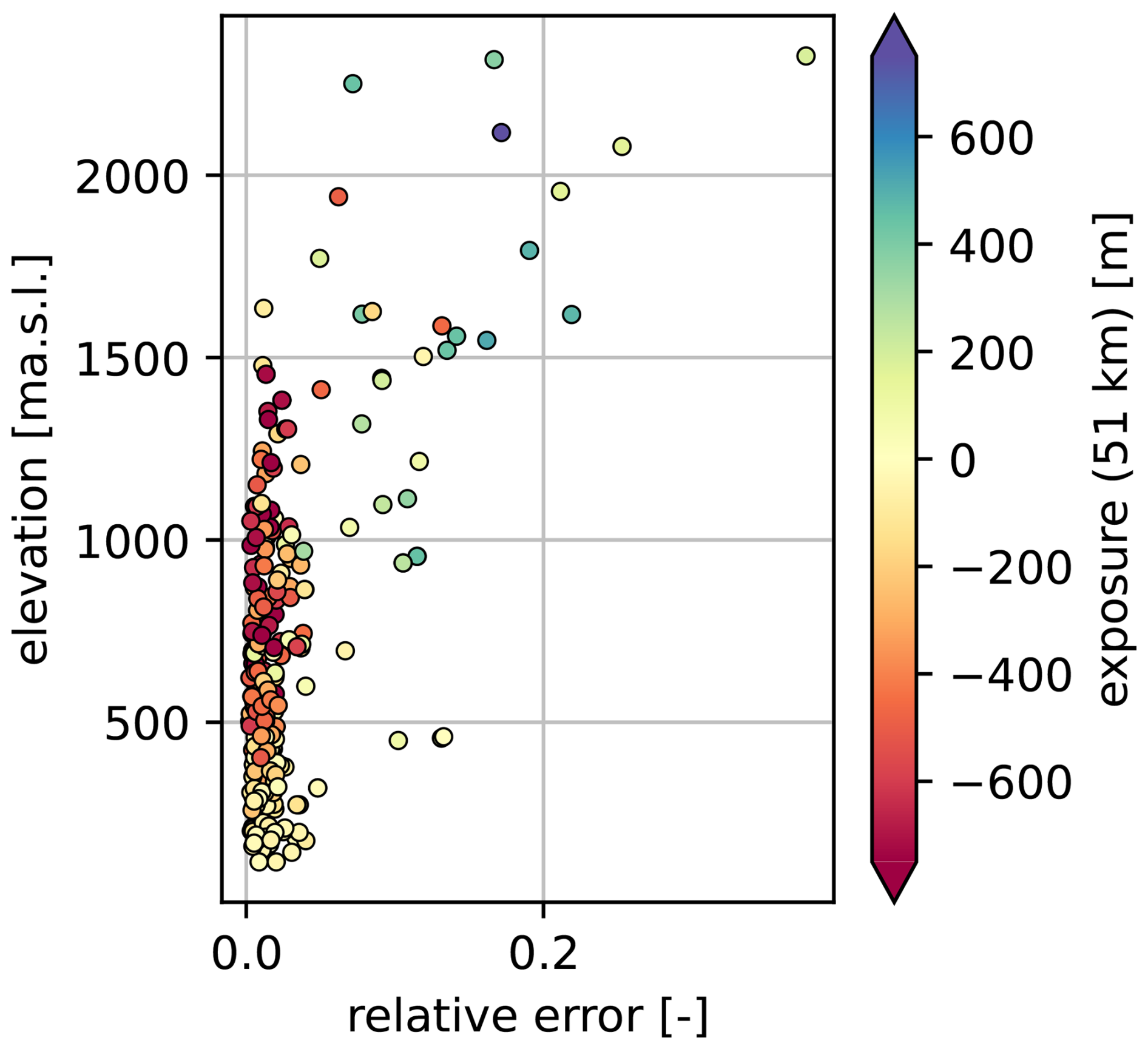
Figure 7 Relative monthly error of the GAM predictions at the stations, averaged over all months. The vertical axis shows elevation in m a.s.l, the color-coding the exposure in m based on a 51 km smoothed topography.

The twelve trained GAMs show robust performance with small relative errors at low-elevation/low-exposure stations, but increasingly struggle to predict undercatch factors at highly-elevated and exposed stations. This confirms the conclusions drawn in Kochendorfer et al. (2017a) that the applied transfer function is prone to uncertainty at highly-elevated, exposed stations with complex wind fields. While the GAMs achieve suitable weighted R² values of approximately 0.8, they tend to overestimate undercatch at these stations (Table 1), resulting in unrealistically high precipitation amounts in exposed, high-alpine terrain. Figure 7 and S3 further illustrate that capping the GAM-predicted undercatch factors at the observed station factors (both shown in Table 1) is a crucial step to prevent excessive extrapolation at high elevations. This is particularly important given the sparse station network at high elevations where the GAMs must extrapolate beyond well-constrained training data.

The feature selection highlighted terrain elevation and geographical exposure (based on a 5 and 51 km smoothed topography) as dominant predictors. Although exposure exhibits concurvity with elevation at high altitudes, it primarily captures small-scale variability, resulting in smooth functions with higher curvature (Fig. 6). Terrain elevation emerges as the primary descriptor of undercatch, exhibiting a near-exponential relationship with undercatch factors (Figs. 6 and S3). In contrast, neither exposure predictor shows a simple monotonic relationship with undercatch. The absence of spatial predictors such as latitude, longitude, or distance to the Alpine main ridge suggests that horizontal proximity alone is insufficient for representing undercatch variability. This suggests that methodologies like ordinary Kriging are impractical to extrapolate undercatch errors.

We conclude that the GAMs produce physically plausible smooth functions that realistically capture the seasonal and elevation-dependent structure of precipitation undercatch, supporting the application of the derived factors to gridded precipitation data. While some model artifacts attributable to predictor concurvity remain, the overall form of the smooth functions, their seasonal variation, and the dominant dependence on terrain elevation are consistent with findings from previous studies (Avanzi et al., 2021; Herrnegger et al., 2018; Pulka et al., 2024). Importantly, unlike these studies – which derived elevation-dependent corrections from additional in situ or satellite snow depth observations or from rainfall–runoff modeling – our approach relies solely on correcting existing meteorological station data, yet arrives at similar conclusions. Our methodology extends previous work in two key aspects: first, by replacing stepwise linear (Pulka et al., 2024; Herrnegger et al., 2018) or exponential fits (Avanzi et al., 2021) with more flexible smooth functions that better capture nonlinear relationships; and second, by providing a more detailed representation of seasonal variability through monthly correction functions, rather than a simple separation into summer and winter conditions (Herrnegger et al., 2018).

3.3 Precipitation Climatologies

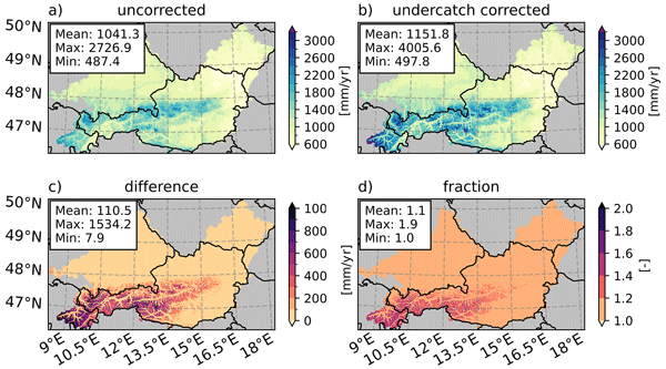
Figure 8 shows the precipitation climatologies for 1991–2020 without undercatch correction (Fig. 8a) and with (Fig. 8b) undercatch correction, their absolute difference (Fig. 8c), all in mm yr⁻¹, and their ratio (Fig. 8d). Undercatch correction leads to a domain-wide increase in precipitation, with a mean increase of 110.5 mm yr⁻¹ across the full domain. The largest absolute increases occur in the alpine regions of western Austria, where precipitation increases locally exceed 1500 mm yr⁻¹, corresponding to a correction factor of 1.9. The maximum undercatch corrected annual precipitation exceeds 4000 mm yr⁻¹, representing an increase of approximately 47 % compared to the uncorrected maximum of 2726.9 mm yr⁻¹.

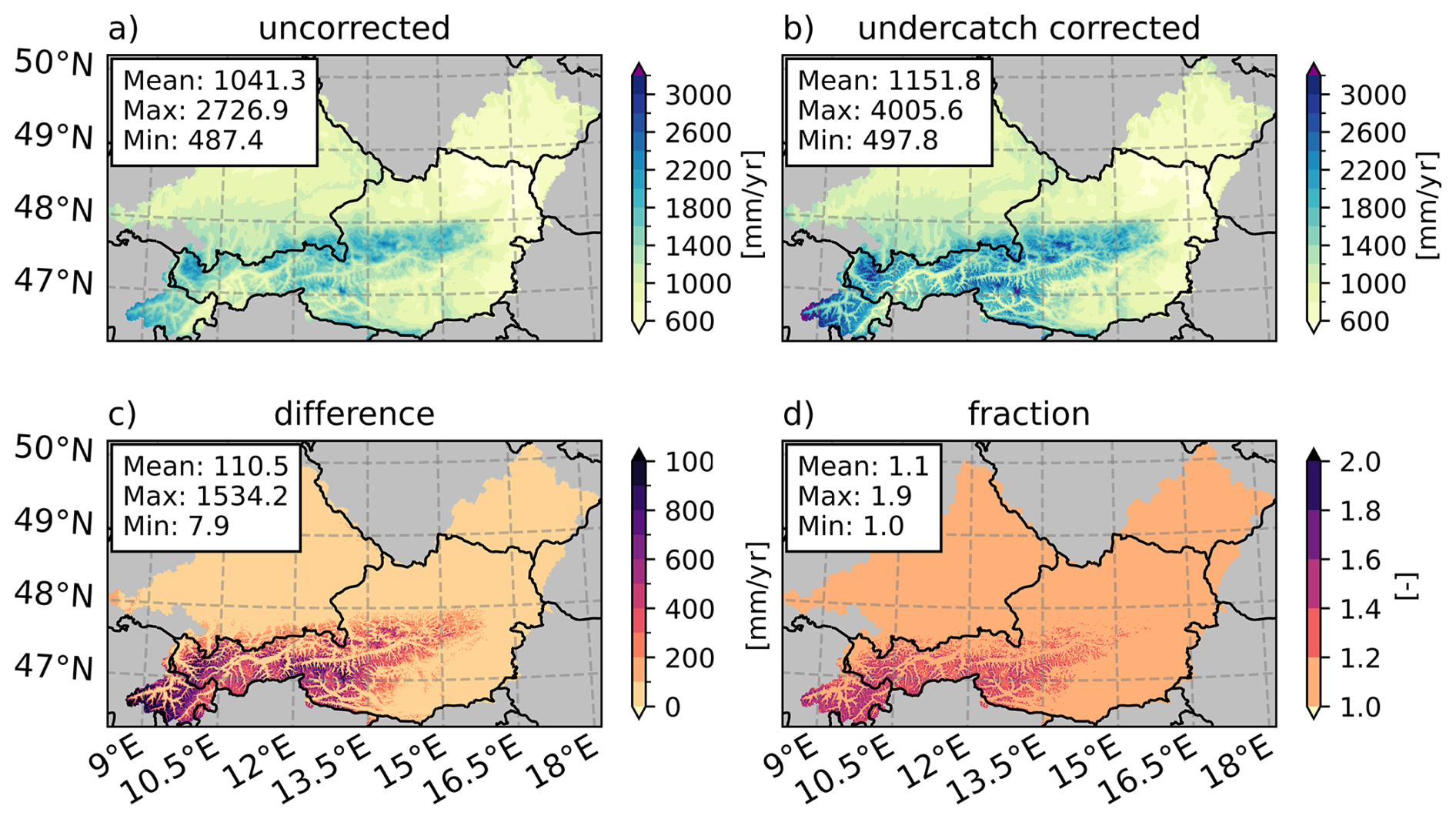
Figure 8 Precipitation climatologies (1991–2020) of (a) uncorrected (b) undercatch corrected and precipitation amounts. Panel (c) shows their absolute difference and (d) their fraction. The first three panels are given in mm yr⁻¹, the last is dimensionless. The mean, maximum and minimum values per panel are given in the text boxes.

Figure 9 shows the local precipitation lapse rates of the undercatch corrected precipitation climatology on a 9 km × 9 km basis in % per 100 m elevation gain. These lapse rates serve as a plausibility check of the corrected precipitation fields. Grid cells shown in white were masked because the local elevation range was insufficient for a meaningful calculation (less than 500 m), or because fewer than half of the 81 grid cells within the window contained valid data. At the highest elevations, lapse rates plateau and locally decrease (yellow colors), which is a direct consequence of the exposed terrain penalty. The mean precipitation increase across Austrian stations is approximately 33 mm per 100 m, corresponding to around 3 % per 100 m when normalized by the mean precipitation of our study domain (Fig. 8a). This is slightly lower than the mean lapse rate of 4.0 % per 100 m shown in Fig. 9, but remains within a plausible range when taking into account the strong corrections in the alpine regions. Since precipitation lapse rates are spatially diverse and vary across the Alpine region due to slope and shielding effects modifying the precipitation-elevation relationship (Frei and Schär, 1998; Dura et al., 2024), individual grid cells are difficult to verify directly. Enhanced lapse rates in regions of strong orographic lifting north of the Alpine main ridge, including the area where the maximum value occurs, appear plausible. However, the high values found in the comparatively dry deep valleys of western Austria, ranging between 7 % and 10 % per 100 m, may indicate local overestimation. This interpretation is supported by comparing these values with the lapse rates between the stations Innsbruck Flughafen and Patscherkofel (see Fig. S1), which are located in close proximity to each other at a valley floor and a mountain crest. Based on transfer-function undercatch-corrected mean annual precipitation, this station pair yields an average annual lapse rate of 4.1 % per 100 m, considerably lower than the highest local values in the gridded field.

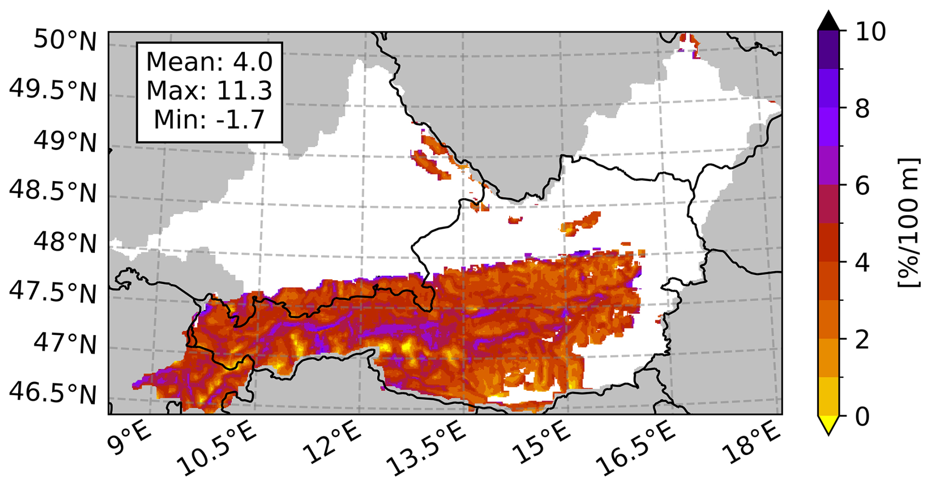
Figure 9 Local precipitation lapse rates of the undercatch corrected precipitation climatology in % per 100 m on a 9×9 km basis. Gray areas mark no or too little surrounding data, whereas white areas show too flat regions for reasonable calculations (less than 500 m elevation range). Mean, maximum and minimum values are given in the text box.

The monthly climatologies, averaged for the full domain and the study regions (see Fig. 1), are shown in Fig. 10a. Undercatch corrected precipitation is displayed as solid lines, while uncorrected data is shown as dashed lines. Figure 10b shows the fraction of corrected and uncorrected monthly precipitation. The strongest relative increase occurs during the winter months. Both high-alpine study regions exhibit a similar annual precipitation increase of approximately 29 %, reflecting their comparable elevation distributions, while the domain-wide mean increase amounts to 10.6 %. A pronounced peak is visible in November in the case study climatology, even though the correction factor of approximately 1.6 is similar to the December value. This peak is caused by individual strong months in the precipitation climatology, especially November 2019 with values of 520 mm per month (280 mm per month) in Kölnbrein (Schlegeis), compared to the climatological average of 139 mm per month (106 mm per month). The summer months are only marginally corrected in all cases. Most notably, the correction substantially alters the seasonal structure of precipitation in the two high-alpine study regions. While the uncorrected data exhibits a clear summer precipitation peak in both regions, which is generally in line with findings in alpine regions (Frei and Schär, 1998), the corrected data shows a comparable or higher precipitation peak in winter, with spring and autumn receiving the least precipitation. Analogous seasonality shifts driven by severe undercatch have been reported at wind-prone sites in the Rocky Mountains (Pan et al., 2016), and high-alpine hydrological studies in the Alps have reached similar conclusions (Pulka et al., 2024). However, a reversal of the dominant summer precipitation peak in Alpine catchments represents a novel finding of this study, making the plausibility of the corrected winter precipitation a central focus of the hydrological validation in the following section.

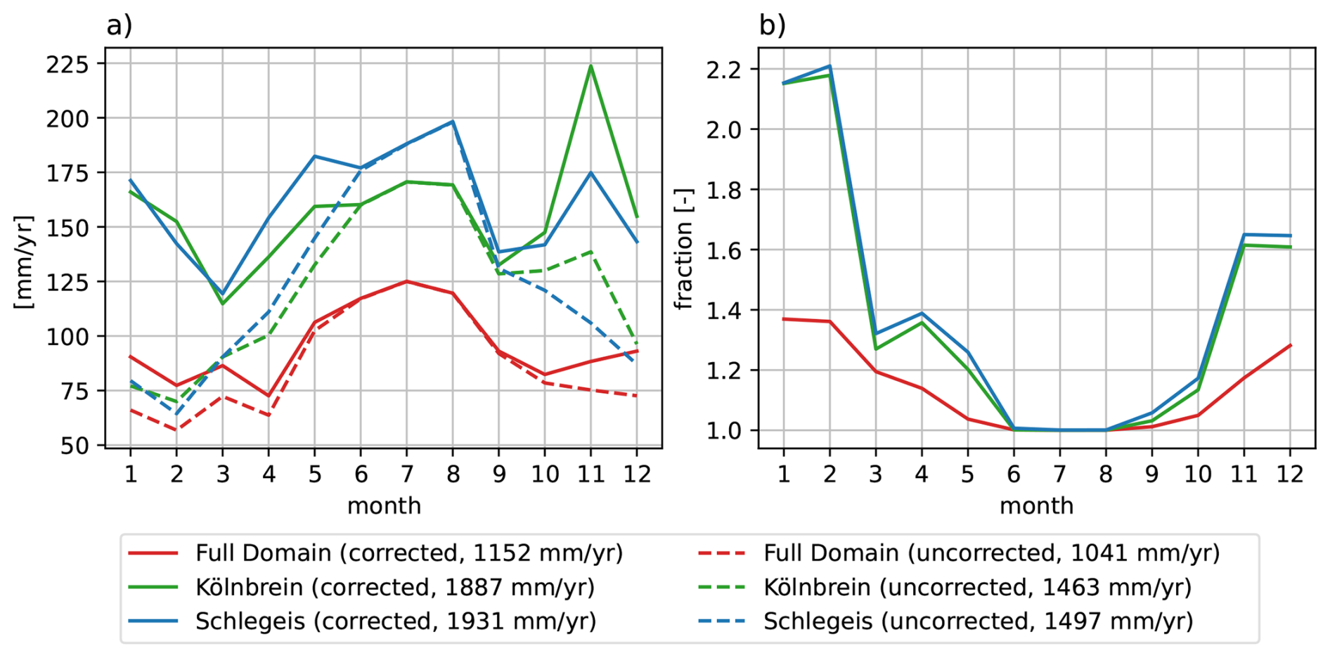
Figure 10 (a) Monthly precipitation climatologies (1991–2020) for the full domain (red) and the study regions Kölnbrein (green) and Schlegeis (blue), both undercatch corrected (solid) and uncorrected (dashed) in mm yr⁻¹ and (b) their fraction. Yearly average precipitation sums are given in the legend.

After initial hydrological validations showed an overestimation of runoff and snow depth likely caused by a too high precipitation correction, an exposed terrain penalty (ETP) is introduced to reduce the precipitation in exposed orography (Fig. 3). The application of the GAM-derived factors and the ETP produces the undercatch corrected precipitation climatologies in Fig. 8. The ETP addresses multiple uncertainties at once: it reduces the potential over-correction of the undercatch transfer function and mitigates the influence of totalizers in the base precipitation data, which dominate interpolation results in high-alpine terrain (Hiebl and Frei, 2018) but generally exhibit lower precipitation measurement errors (Grossi et al., 2017). The precipitation lapse rates (Fig. 9) consequently show the steepest increase starting at slopes close to valley floors and plateau at the highest peaks, mimicking potential flow blocking and moisture depletion (Jiang, 2003; Houze, 2012; Gnann et al., 2025). However, this indicates that some processes in high-alpine, wind-exposed terrain are not fully captured by the transfer function, either because the proposed relationship for the change in catch efficiency is modified by the complex, turbulence-inducing terrain, or the wind speed measurement is not representative of the conditions at the gauge orifice. We therefore conclude that the undercatch correction carries the greatest uncertainty at the highest peaks and that further research specifically targeting precipitation undercatch processes in complex terrain is needed.

3.4 Hydrological Validation

In the following section, the hydrological validation of the undercatch corrected precipitation across different processes and spatial scales is presented. We first evaluate the high-alpine case study regions, where the undercatch errors are expected to be more pronounced and the discrepancies between observed and simulated water balance components (reservoir inflow, snow pack accumulation, glacier mass changes) are especially high. Then the Austrian wide COSERO results will be examined with a focus on runoff quantities.

Figure 11 shows the COSERO simulation results for the two high-alpine reservoir basins Kölnbrein (Fig. 11a, period 2015–2022) and Schlegeis (Fig. 11b, period 2012–2022) as long-term cumulative water balances. The individual components are displayed for simulations using uncorrected (dashed) and undercatch corrected (solid) precipitation input and compared against the observed reservoir inflow (black solid line). Both study regions show substantial improvements in closing the water balance when using the undercatch corrected precipitation. The runoff deficits of 24 % in Kölnbrein (2082 mm yr⁻¹ observed runoff) and 20 % in Schlegeis (1926 mm yr⁻¹ observed runoff) are reduced to less than 1 % for both study regions (2102 mm yr⁻¹ simulated for Kölnbrein and 1988 mm yr⁻¹ simulated for Schlegeis), while glacier melt and evapotranspiration are not altered considerably and remain within realistic magnitudes. Runoff is only displayed for days with valid runoff records, since the observed timeseries contain missing values. The total simulated runoff is slightly higher (2121 mm yr⁻¹ for Kölnbrein and 2189 mm yr⁻¹ for Schlegeis). The average monthly water balance components are provided in Sect. S5 and highlight the improved runoff simulation in the summer months.

Figure 11 COSERO runoff simulation results, as well as observed runoff, displayed as the cumulative water balance for the high-alpine study regions (a) Kölnbrein and (b) Schlegeis. Solid lines refer to the simulation results using undercatch corrected data, while dashed lines refer to results using uncorrected precipitation input. ^* The runoff is only considered for timesteps with valid runoff observations.

Next, we present the validation of snowpack and glacier mass balance modeling with Alpine3D in the two high-alpine case study areas. Figure 12 compares snow depth on 10 May 2021 derived from the WorldView-2 stereo satellite (Fig. 12c) with the simulated snow depth by Alpine3D using uncorrected (Fig. 12a) and undercatch corrected (Fig. 12b) input data. Figure 12d displays the snow depth distribution of individual grid cells as boxplots. The modeled snow depth on 10 May 2021 is severely underestimated when using uncorrected precipitation data, with a median (mean) bias of −0.87 m (−0.78 m). The use of corrected precipitation data leads to a lower, positive bias of 0.15 m (0.30 m). While the median (mean) simulated and observed snow depths are similar, the range of simulated values (Fig. 12d) shows a larger spread and includes higher values. However, the overall pattern is captured well with a clear elevation-dependent distribution of snow depths, particularly for the undercatch corrected variant.

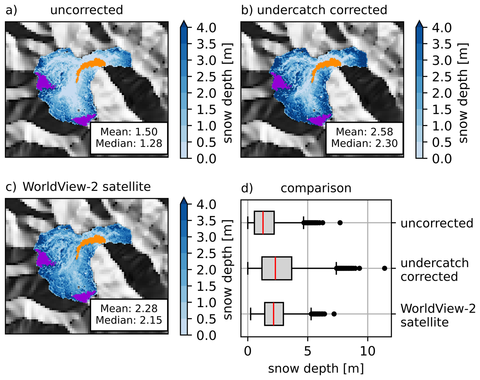
Figure 12 Comparison of satellite-derived and modeled snow depths on 10 May 2021 in the Kölnbrein study region. Displayed is the snow depth in m from Alpine3D modeling results using (a) uncorrected precipitation and (b) undercatch corrected input data and (c) derived from the WorldView-2 stereo satellite image. Spatial mean and median are given in the text boxes. Shaded reliefs are used as background. The violet (orange) area shows the grid cells covered by glaciers (the reservoir). Panel (d) shows a comparison of the spatial variability. The whiskers correspond to the 5th and 95th percentile. Outliers are displayed as dots.

Additionally, the SCA in the Kölnbrein catchment is analyzed during the melting period at different timestamps in 2021. The percentage of SCA based on Sentinel-2 images is compared to the Alpine3D simulations with corrected and uncorrected precipitation input data, as visible in Fig. 13. The SCA of the uncorrected (red) simulation consistently underestimates the SCA observed by Sentinel-2 (black), indicating a too early melt out, i.e. an underestimation of snow amounts. While the undercatch corrected (blue) simulation is closer to the observation throughout all dates, it slightly overestimated the satellite SCA, indicating a too late melt-out in some grid cells, i.e. an overestimation of snow amounts. However, this temporal SCA analysis shows that applying the undercatch corrected precipitation data for the snowpack simulation overall leads to more realistic snow accumulation and melting behavior in 2021. A spatial representation of snow-cover at all four dates, as well as detailed performance metrics, are given in Sect. S6.

Figure 13 Comparison of SCA (%) in the Kölnbrein catchment derived from Sentinel-2 satellite observations and Alpine3D simulations for different dates in the snow-melting period 2021. Compared are Sentinel satellite observations (black), undercatch corrected simulations (blue) and uncorrected simulations (red).

These validations show that the uncorrected precipitation product leads to insufficient snow amounts in the Kölnbrein catchment, as shown exemplarily for 2021 by the underestimation of snow height on 10 May and underestimated SCAs during the melting period. Hence, by undercatch correcting the precipitation (especially in winter months), the simulation of snow melt timing is improved, which in turn leads to an improved fit between simulated and observed runoff (see Sect. S5). The amount of snow and the timing of snow melt subsequently affect the glacier mass balance by determining the date when bare ice first appears and starts to melt. Figure 14 shows the glacier volume change of all glaciers with a surface area greater than 1 km² located in the more heavily glaciated Schlegeis study region for the period 2000–2023 (for details on the selected glaciers see Sect. S7). The Alpine3D simulations are compared to the average volume change (black line) of the same glaciers between 2000 and 2019 derived by Hugonnet et al. (2021), which amounts to a loss of −0.21 km³ (or −0.011 km³ yr⁻¹). The undercatch corrected data (blue line) shows good agreement with the reference data, while the uncorrected precipitation data (red line) leads to too high volume loss. This indicates that an insufficient amount of solid precipitation is covering the glaciers, resulting in a too early onset of ice melt.

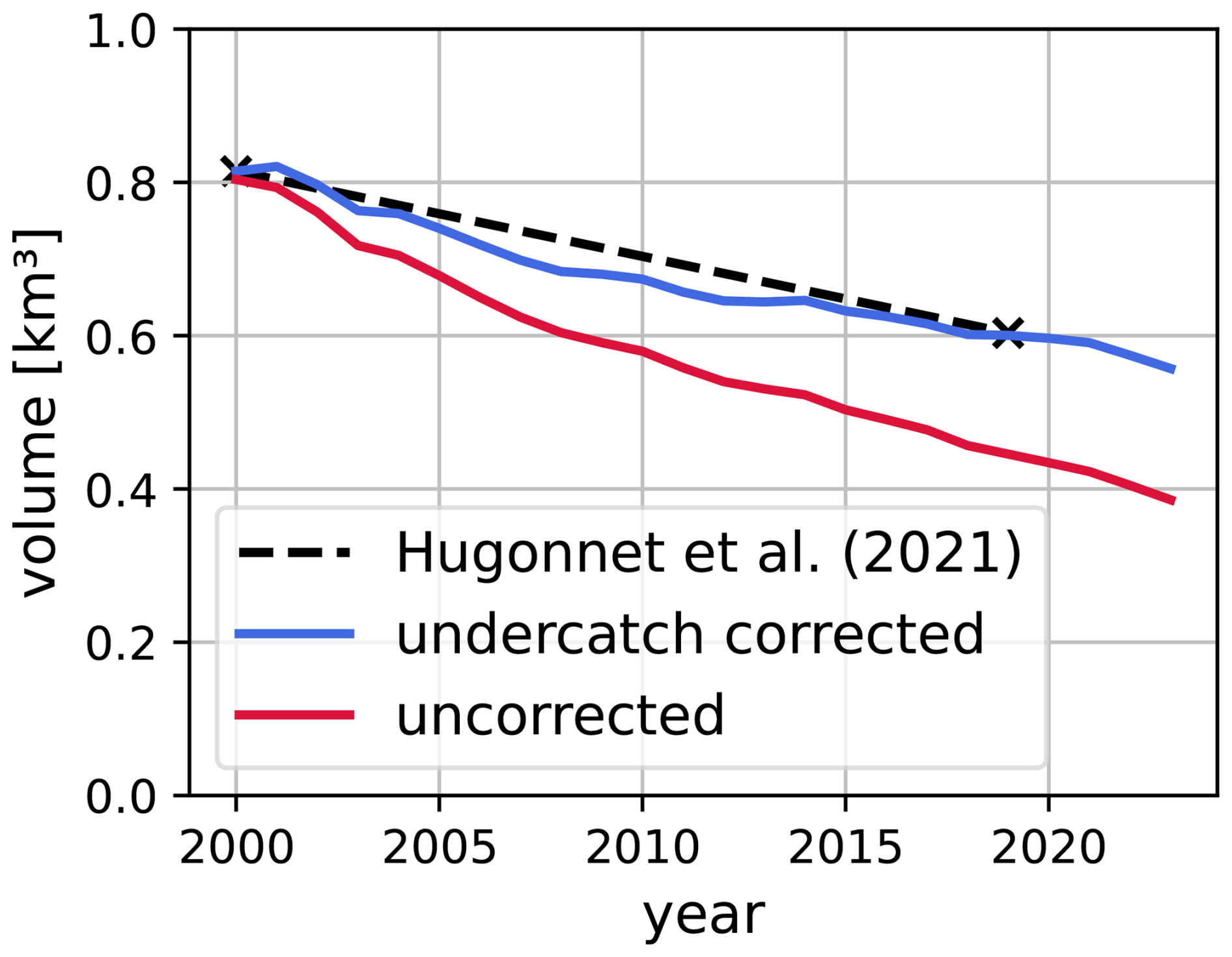
Figure 14 Simulated total glacier volume change for glaciers with a surface area above 1 km² in the Schlegeis study region in km³ from 2000–2023. The undercatch corrected (blue) and uncorrected (red) Alpine3D simulation is compared to the average volume change of the selected glaciers between 2000–2019 as published by Hugonnet et al. (2021), which amounts to a loss of −0.011 km³ yr⁻¹ between 2000 and 2019.

After examining the effects of using the undercatch corrected precipitation data in the case study regions, the product is examined across Austria. Figure 15 shows the calibration results of the COSERO simulations across Austria. Displayed is the bias

$$\begin{array}{}\text{(6)}& \mathit{\beta }={\displaystyle \frac{{\stackrel{\mathrm{‾}}{Q}}_{\mathrm{sim}}}{{\stackrel{\mathrm{‾}}{Q}}_{\mathrm{obs}}}},\end{array}$$

which is the fraction of the long-term simulated and observed mean runoff in the calibration period. The two upper panels display β for simulations using uncorrected (Fig. 15a) and undercatch corrected (Fig. 15b) precipitation input. The uncorrected simulation shows distinct spatial heterogeneities, with the expected runoff underestimation in catchments along the Alpine main ridge. An overestimation can be seen in low-lying catchments in the south, east and north-east. After applying the undercatch correction (Fig. 15b), especially the catchments along the Alpine main ridge are improved, indicated by β≈1, while catchments that already show values of β>1 for uncorrected precipitation naturally show similar biases when applying the undercatch correction. The water balance in these catchments is characterized by high evapotranspiration rates and low precipitation amounts, leading to low annual runoff sums of only a few 100 mm per year or even less. This means that already slight deviations from the observed values lead to poor goodness-of-fit measures, and in this case an overestimation in β. This can also be seen in Fig. 15c, where β is displayed across different elevation bands. The catchments in elevations below 1000 m show median β values above 1 both before and after the correction, and show the overall highest β outliers with values above 4. On the other hand, a significant improvement can be seen for the 39 catchments above 2000 m, where β values are notably below 1 before the correction. Median β values in catchments between 1500 and 2000 m increase from slightly below 1 to slightly above 1. For the entire modeling domain, the median β improves from 1.13 to 1.09 when using the undercatch corrected precipitation input. At first glance, this may appear counterintuitive, as increasing precipitation inputs would be expected to increase simulated runoff and thus β. This behavior stems from the simultaneous calibration approach: when optimizing a single objective function (runoff) across the spatially heterogeneous domain with uncorrected inputs, the algorithm compensates for precipitation deficits in alpine catchments by reducing evapotranspiration rates. While this compensation improves fit in alpine regions, it also exacerbates runoff overestimation in low-lying basins where precipitation deficits are less pronounced. The undercatch correction eliminates this artificial compensation mechanism, yielding more physically consistent water balance estimates and parameter sets across the elevation bands.

Similar figures for two other measures of goodness-of-fit, the Kling–Gupta Efficiency (Gupta et al., 2009) and the Nash–Sutcliffe Efficiency (Nash and Sutcliffe, 1970), can be found in Sect. S8. Both metrics show not only improved median performance (NSE: from 0.50 to 0.54, KGE: from 0.55 to 0.62), but also substantial reduction in the lower tail of the performance distribution, indicating fewer poorly performing catchments. Precipitation and evapotranspiration per elevation band for both model runs are provided in Sect. S9. The undercatch correction increases precipitation inputs in all elevation bands above 1000 m, while precipitation below 1000 m remains largely unchanged. Correspondingly, actual evapotranspiration increases across all elevation zones when using corrected precipitation, reflecting the elimination of artificial ET suppression that previously compensated for input deficits during calibration.

The Austrian-wide COSERO model was independently validated for the period 1980–2000. Using undercatch-corrected precipitation results in slightly improved median performance, with β values of 1.08 (uncorrected) and 1.07 (corrected), NSE values of 0.52 and 0.54, and KGE values of 0.60 and 0.65, respectively. Elevation-dependent validation metrics are provided in Sect. S10. Consistent with the calibration results, improvements are most pronounced in high-elevation catchments, where NSE and KGE distributions shift towards higher values and fewer poorly performing basins are observed.

Figure 15 Runoff bias β for the calibrated subcatchments of the Austrian-wide COSERO model, for simulations using (a) uncorrected and (b) undercatch corrected precipitation, as well as (c) separated into elevation bands. The black outline in panels (a) and (b) shows the subcatchment borders. Numbers in parentheses in panel (c) indicate the number of catchments within each elevation band. Whiskers represent 1.5 times the interquartile range, and outliers are shown as dots.

Overall, the hydrological validation across Austria (Fig. 15) shows an improvement in model biases in alpine catchments when using the undercatch corrected precipitation input. This is demonstrated in the two case study regions by (1) closing the long-term water balance (Fig. 11), (2) improving severe negative mean and median biases in snow depth modeling (Fig. 12), (3) improved representation of snow melt out behavior (Fig. 13), and (4) more realistic glacier volume changes (Fig. 14). The Austrian-wide COSERO simulations show the same elevation-dependent results, with the undercatch correction leading to improved simulation in catchments above 2000 m (Fig. 15). Poor model performance is evident in both the uncorrected and corrected runs for lower-elevation catchments in the south, east, and north-east. This issue could be attributed to: (1) inaccurate precipitation in the base data set (Hiebl and Frei, 2018), (2) shortcomings in the hydrological model and/or its calibration, or (3) shortcomings in the observed runoff data. We assume that the uncertainties related to (3) are on average low, since the data is quality controlled. Therefore, the observed runoff data likely provides reliable information on catchment processes and can be used to diagnose the remaining potential sources of error, namely the model structure/calibration (2) or the precipitation input (1). Runoff overestimation occurs in two distinct regions. First, in southern Austria along the Gail and Drau (Drava) rivers and their tributaries, which exhibit pluvial-nival regimes with spring maxima (April) and secondary winter peaks (November). This spatial bias cannot be attributed to regime type alone, as the model performs well for catchments with similar regimes in the northern Alpine foothills (e.g., Danube tributaries Ybbs, Erlauf, and Pielach). The overestimation in the south likely reflects either regional biases in the base gridded precipitation dataset (Hiebl and Frei, 2018), unresolved spatial processes during GAM training, or distinct weather regimes affecting northern versus southern Austria (Bozzoli et al., 2024; Haslinger et al., 2025). Signed distance to the Alpine main ridge was not selected as a predictor during model development, which suggests that the north-south differences may stem from atmospheric processes that cannot be adequately represented by topographic variables alone. The second region with systematic runoff overestimation covers the eastern and northeastern catchments along the Raab and Thaya rivers and their tributaries. These lowland areas exhibit pluvial regimes with a single runoff peak in early spring (March), low annual runoff totals, high air temperatures, and consequently high evapotranspiration rates. The poor model performance in these catchments likely stems from multiple compounding factors: (i) the simultaneous domain-wide calibration strategy inadequately captures the distinct hydrological behavior of these low-gradient systems, particularly their flashy response characteristics and actual evapotranspiration; and (ii) observational uncertainty is highest in these catchments due to measurement challenges at low flow volumes, potentially providing unreliable calibration targets. Runoff underestimation is evident in basins located in the central regions of Austria, north of the Alpine main ridge. This is plausible given that these are karstic regions where orographic catchment boundaries do not necessarily coincide with hydrological catchment boundaries, and underground flow paths may be neglected in the model. Additionally, natural or anthropogenic diversions may not be adequately represented in the model structure despite careful consideration, potentially causing discrepancies between observed and modeled runoff.

Two further sources of overall uncertainty merit discussion. First, actual evapotranspiration (ETA) is difficult to validate due to the scarcity of measurements, particularly at the regional scale. COSERO estimates potential evapotranspiration (ETP) using the Thornthwaite method (Thornthwaite and Mather, 1957) and calculates actual evapotranspiration from interception and soil storage, as well as snow sublimation. In the calibration process, ETA is not constrained, meaning it may be adjusted to close the water balance and improve the objective function, potentially resulting in implausible values. While we verified that spatial patterns and approximate quantities fall within a plausible range, uncertainties remain. Future research could address this by constraining ETA using satellite-derived products such as the Global Land Evaporation Amsterdam Model (GLEAM, Miralles et al.,2011). Second, the strong topographic and hydrological heterogeneities across Austria likely prevent a simultaneous, all-in-one calibration routine from identifying optimal parameters for every region, potentially leading to poor performance in some catchments. Using an optimization routine that relates model parameters to landscape properties, thereby retaining physical process realism (e.g. Samaniego et al., 2017; Feigl et al., 2022), could be a topic for further research.

3.5 Limitations

Overall, the proposed methodology for generating undercatch-corrected gridded precipitation performs well across Austria. Nevertheless, several limitations remain and should be considered when interpreting the results:

• The undercatch transfer function from Kochendorfer et al. (2017a) showed reduced accuracy in precipitation measurement at the only high-alpine calibration station in their study. This indicates limited applicability of the catch efficiency function in Austria's high-alpine complex orography. This necessitated the introduction of the exposed terrain penalty in our study and highlights the need for further research to better understand processes influencing precipitation undercatch in high-alpine terrain.

• Several snow-related processes are not explicitly considered at the 250 or 1000 m grid resolution, including wind-driven snow redistribution and ablation (Mott et al., 2018), blowing snow sublimation (Vionnet et al., 2014; Sigmund et al., 2025), and canopy-snow interactions (Hedstrom and Pomeroy, 1998). While these processes may contribute to precipitation uncertainty, they are neglected in this study.

• The base precipitation dataset combines measurements from tipping buckets and totalizers (Hiebl and Frei, 2018), which exhibit different undercatch characteristics. Since totalizers show smaller measurement errors than tipping buckets (Grossi et al., 2017), regions with high totalizer weights in the spatial interpolation receive inflated precipitation values after undercatch correction, resulting in localized overestimations. This affects the dataset used in this study and manifests as maximum values exceeding 4000 mm yr⁻¹ in individual grid cells.

• The hydrological validation revealed potential limitations and inaccuracies in the base precipitation data (Hiebl and Frei, 2018), particularly in southern Austria near the border. Future versions of this data set may benefit from including these findings for specific regions with larger offsets.

• The methodology is suitable for climate model data only if it was bias-adjusted using uncorrected station-based historical data. Through bias adjustment, the undercatch errors of the observations are propagated into future projections, allowing the use of the same undercatch corrections derived in this study. These correction factors should consequently not be applied to raw climate projection data.

• Beyond precipitation uncertainty, additional sources of error include other meteorological driver data, potential model structural errors in both COSERO and Alpine3D, and uncertainties in the reference datasets used for validation. While results demonstrate clear improvements from undercatch correction, we cannot entirely exclude the possibility of obtaining correct results through compensating errors, particularly in high-alpine catchments.

4 Conclusions

In this study, we demonstrate that retrospective correction of commonly used gridded precipitation data for undercatch errors is essential for accurate hydrological modeling in high-alpine regions. We present a reproducible methodology that combines meteorological station observations, an established undercatch transfer function, and Generalized Additive Models informed by terrain characteristics. This approach resulted in publicly available undercatch correction factors (Maier et al., 2025), which were subsequently used to derive a novel precipitation climatology for Austria and adjacent headwater catchments that explicitly accounts for precipitation undercatch at the station level. The undercatch corrected precipitation data was extensively validated using hydrological and snowpack simulations across a range of spatial and temporal scales, hydrological processes, and elevation bands. The results show that undercatch correction is particularly critical for snow-hydrological modeling and other applications in high-alpine terrain, where uncorrected precipitation leads to systematic biases and reduced agreement with observations. Incorporating undercatch correction substantially improves the consistency between simulated and observed runoff, snow cover, and glacier mass changes. Despite these improvements, remaining uncertainties – especially in wind-exposed and highly complex mountain terrain – highlight the need for further research into precipitation undercatch processes.

The framework presented here is generalizable and can be reproduced in other mountain regions, provided that the following requirements are met: (i) comparable (high-elevation) station coverage, (ii) sufficient observation quality, and (iii) DEM and gridded precipitation data that adequately resolve the spatial scale of the underlying orography. The latter requirement is particularly important, as strongly smoothed DEMs can fail to represent small-scale topographic characteristics and may affect elevation-dependent precipitation estimates in complex high-alpine terrain (Weber et al., 2021). Where these conditions are fulfilled, we encourage the application of the proposed methodology to other mountain regions and gridded precipitation datasets to advance the understanding of undercatch errors across diverse climatological and topographic settings. Additionally, future work should evaluate alternative undercatch correction approaches systematically, in a similar structure as proposed by Aubry et al. (2025), for example by considering correction methods that rely on snowfall intensity rather than on air temperature. Further, greater emphasis should be placed on improving the physical representation of undercatch. This could be achieved through advanced modeling approaches that couple Lagrangian models (e.g. Bakels et al., 2024) and moisture and precipitation tracking frameworks (e.g. Sodemann et al., 2008) with high-resolution snowpack simulations, as well as through enhanced experimental observations at high-elevation and exposed sites. Such developments are essential to further reduce uncertainty in alpine precipitation estimates and to improve the reliability of hydrological projections in a changing climate.