Explicit representation and calibration of different landscape units for a robust catchment DOC export model

Elevated dissolved organic carbon (DOC) concentrations are a major concern for ecosystems and drinking water supply. Data-driven studies revealed variable functioning of different landscape units (upland, riparian zone, and groundwater) in catchment DOC mobilization and export. However, lumped and landscape-explicit (separating upland and riparian zone) model structures are generally calibrated to stream DOC concentrations, while the internal DOC dynamics often do not receive sufficient attention. Here, we developed a flexible model with a lumped and landscape-explicit structure for four headwater catchments in the Harz Mountains, Germany. We evaluated these models under a baseline calibration (only against stream DOC concentration) and a constrained calibration (using stream DOC and internal DOC concentrations). Under the baseline calibration, both model structures reproduced stream DOC dynamics with acceptable performance in some catchments (Kling–Gupta efficiency of behavioural simulations>0.6), but with unrealistically high groundwater DOC. By contrast, the constrained calibration reduces the KGE for stream DOC concentrations but produces internal DOC dynamics consistent with the imposed observational and process-based constraints. Additionally, the landscape-explicit model structure is more robust than the lumped model structure under changing boundary conditions. Our study thus shows that robust catchment DOC modelling requires not only explicit representation of different landscape units, but also calibration constraints based on DOC concentrations within those units.

1 Introduction

Dissolved organic carbon (DOC) plays a crucial role in aquatic ecosystems, providing carbon and energy for microbial metabolism (Kaplan and Newbold, 2000; Mulholland, 2003). The amount of DOC in drinking water reservoirs, however, can be of concern as DOC can interact with chlorine used for drinking water disinfection and form harmful disinfection by-products (Bond et al., 2014). In surface water bodies, the main source of DOC is soil organic matter in terrestrial landscapes, i.e., allochthonous carbon (Mitrovic and Baldwin, 2016). Having a robust tool to quantify catchment DOC mobilization from its terrestrial sources to the river and to predict its response to changing boundary conditions has long been a research goal (Wei et al., 2024). Such tools and derived knowledge are important for water quality management, especially in headwater catchments that play a pivotal role in defining the quality of downstream water resources (Alexander et al., 2007).

Data-driven studies in headwater catchments have shown that the amount of DOC exported from different landscape units (the upland and riparian zone) to the stream is disproportionate to their area fractions within a catchment (Bishop et al., 2004; Blaurock et al., 2022; Dosskey and Bertsch, 1994; Ledesma et al., 2015; McGlynn and McDonnell, 2003). Often, the riparian zone is much smaller in area than the upland, but acts as the main source of stream DOC (Musolff et al., 2018; Strohmeier et al., 2013). Riparian zones in temperate and boreal systems cover a large portion of the Earth's land surface and exhibit DOC dynamics that are broadly applicable across other systems. They are typically wet with shallow groundwater levels, rich in organic matter, enhancing lateral hydrological connectivity between the DOC source zone and the stream network (Ledesma et al., 2018a). The minor contribution of the upland DOC to stream DOC is argued to be due to a lack of direct hydrological connectivity between the organic layers of the upland soils and the stream. In the upland, DOC is transported vertically from the organic-rich, narrow upper soil layers into the deeper dominant mineral subsoil and quickly gets adsorbed to the mineral phase, resulting in low DOC concentrations in the percolating water that recharges the groundwater (Kothawala et al., 2012; Ledesma et al., 2018a; Sierra et al., 2013). Therefore, the groundwater that flows into the riparian zone is low in DOC. In consequence, not all soil organic matter in a catchment is relevant for the exported DOC, but rather the fraction that can be hydrologically connected via short lateral flow paths (Zarnetske et al., 2018; Ebeling et al., 2021).

Although data-driven studies highlighted these distinct roles of the upland and riparian zones in shaping stream DOC concentrations and their dynamics, DOC modelling approaches often do not explicitly distinguish the upland and riparian zones in model structures. For example, hillslope (or lumped) model conceptualizations often consider a catchment as a single landscape unit (no separation between the upland and riparian zone) with two or more vertical layers representing the upper soil and lower soil or groundwater (Birkel et al., 2017; Grieve, 1991; Michalzik et al., 2003). Established semi- and fully-distributed water quality models such as the Soil and Water Assessment Tool model for Carbon (SWAT-Carbon; Arnold et al., 1998; Mukundan et al., 2023), the Hydrological Predictions for the Environment model (HYPE; Pers et al., 2016), and the Integrated Catchments model for Carbon (INCA-C; Futter et al., 2007) exhibit detailed descriptions of how DOC is formed from soil organic matter and interacts with external inputs from plants under given temperature and soil moisture conditions. The SWAT and INCA-C models, however, do not represent the upland or riparian compartments explicitly; instead, the catchments are represented by discrete, hydrologically disconnected units (e.g., grid cells or hydrological response units). The HYPE model has an option to represent the riparian zone (primarily designed for forest land) as an infinite DOC source to increase DOC concentrations from soil runoff before entering the stream (SMHI, 2026). However, none of the above models combine explicit landscape units with the representation of DOC processes within those landscape units.

In contrast to the aforementioned models, several others allow an explicit representation of upland and riparian zones, e.g., the modified version of the Lund-Potsdam-Jena dynamic global vegetation model and General Ecosystem Simulator (LPJ-GUESS, Tang et al., 2018; Smith et al., 2001), the ECOsystem 3D (ECO3D, Liao et al., 2019), and the DOC model developed by Birkel et al. (2014). The LPJ-GUESS and ECO3D are fully distributed and grid-based models that allow detailed representation of hydrological and DOC processing and flow routing among grid cells. These models, however, require high computational resources and are challenging to parameterize as well as to evaluate (Birkel et al., 2014; Tang et al., 2018). The simpler model developed by Birkel et al. (2014) allows the discretization of catchments into the upland, riparian, and groundwater compartments in a semi-distributed (not gridded) manner. Hereinafter, we refer to this type of discretization as a landscape-explicit model structure. However, in contrast to LPJ-GUESS and ECO3D, the Birkel et al. (2014) model strongly simplifies soil DOC formation and does not allow for closing carbon mass balances.

The existence of multiple model structures (Wei et al., 2024) for simulating stream DOC concentrations regardless of whether these models separate different landscape units raises the questions: (1) are lumped and landscape-explicit model structures both able to produce the right results (i.e., acceptable simulations of stream DOC concentrations at the catchment outlet) for the right reasons (i.e., realistic simulations of internal DOC concentrations) (Kirchner, 2006) when they are calibrated against stream DOC concentration only? and (2) what is the value of a constrained calibration in which information on DOC concentrations of different landscape units is used in addition to stream DOC concentrations for improving the model's credibility and physical soundness? Several studies (e.g., Bouaziz et al., 2021; Wu et al., 2023) demonstrated that calibrating a model only using the integrated signal at the catchment outlet does not guarantee plausible internal modelled results. These studies call for the utilization of additional data, such as soil moisture or stable water isotope observations, to constrain the model and avoid implausibility or inconsistency. However, while the value of additional data has been demonstrated for models focusing on water quantity, applications for water quality models have been rare. Sarrazin et al. (2022) showed the value of additional “soft” data in reducing equifinality in the parameterization of a water quality model focused on catchment nitrogen transport and fate. To the best of our knowledge, the two aforementioned research questions remain unanswered in the context of DOC modelling.

The objective of this study is, therefore, to address these two research questions on the internal consistency and value of additional data for catchment DOC models. For that, we developed lumped and landscape-explicit DOC structures in a modular DOC model, combining the strengths (model structure and DOC processes representation) of two existing models (Birkel et al., 2014; Futter et al., 2007). We then applied the proposed models in four intensively studied catchments in the Harz Mountains, Germany as a demonstrative example. Although the four selected catchments are located within a specific region, they are part of broader comparative effort to assess riparian state and functioning across established experimental catchments (Ledesma et al., 2025; Trojahn et al., 2026). We evaluated whether the two model structures produced realistic internal DOC concentrations under a baseline calibration (against stream DOC concentration only) and a constrained calibration (using stream DOC concentration and internal DOC concentration). Furthermore, we conducted a structural stress test in which the two model structures (lumped and landscape-explicit) were subjected to changing boundary conditions to assess the robustness and plausibility of their simulated stream DOC responses. Ultimately, our study aims to provide insights into model selection, calibration, evaluation, and application for water quality management.

2 Methodology

2.1 DOC Modelling approach

The DOC model developed in this study is a catchment-scale model operating at a daily timestep (Fig. 1). It uses hydrological states and fluxes from the mesoscale Hydrologic Model (mHM; Kumar et al., 2013; Samaniego et al., 2010). As the DOC and mHM models operate at different spatial scales, hydrological fluxes and states from mHM were first aggregated from the grid to the catchment scale using area-weighted averaging and then disaggregated using area-weighted allocation to the landscape units of the DOC model (Sect. S1 in the Supplement). The model simulates carbon (C) transformation, balance, and C pools for each model compartment.

Figure 1 Conceptual representation of (a) the lumped model structure, (b) the landscape-explicit model structure, and (c) the carbon transformation among different carbon pools.

We developed a flexible model structure, in which lumped and a landscape-explicit model structure can be switched on and off. Both model structures are accessed through a single executable file, and users can select which one to use in the configuration file. The lumped model structure considers a combined upland and riparian zone as a single compartment plus an additional groundwater compartment (Fig. 1a), and the landscape-explicit model structure considers upland, riparian, and groundwater compartments separately (Fig. 1b). The groundwater compartment in the lumped model structure receives vertical inputs from the hillslope, which combines both upland and riparian zone into a single unit. By contrast, in the landscape-explicit model structure, the groundwater compartment receives inputs only from the upland. The groundwater compartment in both model structures represents the deeper layer of water flow and solute transport to the stream below the active soil layer. The lumped and landscape-explicit model structures are similar to those developed by Birkel et al. (2017) and Birkel et al. (2014), respectively. In contrast to Birkel et al. (2014), groundwater in our landscape-explicit model structure can flow (a) directly to the stream, reflecting regional, deep groundwater flow, and (b) via a riparian zone, reflecting local, shallow groundwater flow (Laudon and Sponseller, 2018; Tóth, 1963).

Representation of the C transformation processes in both model structures is based on the INCA-C model (Futter et al., 2007) that considers three C pools (immobile pool: soil organic carbon – SOC; mobile pools: dissolved inorganic carbon – DIC, and DOC) in the hillslope, upland, and riparian zone (Fig. 1). The transformation rates between C pools depend on soil temperature and soil moisture:

$$\begin{array}{}\text{(1)}& {\displaystyle }& {\displaystyle }{k}_{x\to y,z}\left(t\right)=k_{x\to y,z}^{\mathrm{0}}\cdot {\mathit{\eta }}^{\left(T_{\text{soil}}\right(t)-\mathit{\theta })/\mathrm{10.0}},\text{(2)}& {\displaystyle }& {\displaystyle }{k}_{x\to y,z}\left(t\right)=k_{x\to y,z}^{\mathrm{0}}\cdot {\displaystyle \frac{({\text{SMD}}_{\text{max}}-\text{SMD}(t\left)\right)}{{\text{SMD}}_{\text{max}}}},\end{array}$$

where k⁰ (–) is the base rate, the subscripts x and y indicate the type of C pool (SOC, DIC, or DOC), z indicates upland (UL) or riparian zone (RZ) in the landscape-explicit model structure, or the hillslope (HS) in the lumped model structure (e.g., $k_{\text{SOC}\to \text{DOC,UL}}^{\mathrm{0}}$ (d⁻¹) is the base transformation rate from SOC to DOC in the upland), t (d) is time, η (–) is the soil temperature multiplier, θ (°C) is the base temperature offset, SMD (mm) is soil moisture deficit depending on the field capacity (FC) and current soil moisture, SMD_max is the maximum SMD – the driest condition (calibrated threshold value) at which transformation between different carbon pools can take place, and T_soil (t) (°C) is soil temperature. Soil temperature at day t is calculated based on the mean antecedent air temperature on the previous n days, as follows:

$$\begin{array}{}\text{(3)}& T_{\text{soil}}\left(t\right)={\displaystyle \frac{{\sum }_{i=t-n}^t{T}_{\text{air}}\left(i\right)}{n+\mathrm{1}}},\end{array}$$

where T_air(i) (°C) is the daily mean air temperature at day i ($i=t-n,t$), and n is the model parameter. This method was demonstrated to be effective in approximating soil temperature from air temperature in the study area (Fig. S1 in the Supplement).

We represent the net transformation between SOC and DOC using an effective transformation rate ($k_{\text{SOC}\to \text{DOC},z}\left(t\right)$) instead of representing the transformation of DOC to SOC and SOC to DOC explicitly, like the INCA-C model, or sorption of DOC on soil (e.g., Wen et al., 2020). This simplification assumes a net transfer of SOC to DOC and aims to reduce equifinality as data to evaluate the internal transformation pathways and its associated parameter is typically not available, at least in our study area (Sect. 2.2).

In the groundwater compartment, we consider the two soluble C pools (DIC and DOC) and the transformation from DOC to DIC, but no SOC and no inputs from litterfall and root breakdown. The transformation rate from DOC to DIC is not constrained by soil moisture and temperature, as this is a fully saturated zone and groundwater temperature varies minimally throughout the year.

The SOC balance equations for the UL, RZ, and HS are:

$$\begin{array}{}\text{(4)}& \begin{array}{rl}{\displaystyle \frac{\partial M_{\text{SOC},z}\left(t\right)}{\partial t}}=& {\displaystyle }{f}_z\cdot \left({\text{LF}}_z\right(t)+{\text{RB}}_z(t\left)\right)-m_{\text{SOC}\to \text{DOC},z}\left(t\right)\\ {\displaystyle }& {\displaystyle }-m_{\text{SOC}\to \text{DIC},z}\left(t\right),\end{array}\end{array}$$

where the subscript z indicates the upland (UL) or riparian zone (RZ) in the landscape-explicit model structure, or the hillslope (HS) in the lumped model structure, M (kg ha⁻¹) is the SOC mass in the hillslope, upland, or riparian zone, m ($\mathrm{kg}{\mathrm{ha}}^{-\mathrm{1}}{\mathrm{d}}^{-\mathrm{1}}$) is the C flux transferred between different C pools, f (–) is the areal fraction of the hillslope (f_HS), upland (f_UL), or riparian zone (f_RZ) within a catchment (lumped model structure: f_HS=1), LF and RB ($\mathrm{kg}{\mathrm{ha}}^{-\mathrm{1}}{\mathrm{d}}^{-\mathrm{1}}$) are litterfall and root breakdown, respectively. LF occurs at a user-specified period of the year, and RB occurs throughout the year at a constant rate (Futter et al., 2007).

The DOC balance equations for the HS and GW of the lumped model structure are:

$$\begin{array}{}\text{(5)}& {\displaystyle }& {\displaystyle }\begin{array}{rl}{\displaystyle }& {\displaystyle \frac{\partial M_{\text{DOC,HS}}\left(t\right)}{\partial t}}=m_{\text{SOC}\to \text{DOC,HS}}\left(t\right)-m_{\text{DOC}\to \text{DIC,HS}}\left(t\right)\\ {\displaystyle }& {\displaystyle }-m_{\text{DOC,HS}\to \text{STREAM}}\left(t\right)-m_{\text{DOC,HS}\to \text{GW}}\left(t\right),\end{array}\text{(6)}& {\displaystyle }& {\displaystyle }\begin{array}{rl}{\displaystyle }& {\displaystyle \frac{\partial M_{\text{DOC,GW}}\left(t\right)}{\partial t}}=m_{\text{DOC,HS}\to \text{GW}}\left(t\right)-m_{\text{DOC}\to \text{DIC,GW}}\left(t\right)\\ {\displaystyle }& {\displaystyle }-m_{\text{DOC,GW}\to \text{STREAM}}\left(t\right),\end{array}\end{array}$$

The DOC balance equations for the UL, RZ, and GW of the landscape-explicit model structure are:

$$\begin{array}{}\text{(7)}& {\displaystyle }& {\displaystyle }\begin{array}{rl}{\displaystyle }& {\displaystyle \frac{\partial M_{\text{DOC,UL}}\left(t\right)}{\partial t}}=m_{\text{SOC}\to \text{DOC,UL}}\left(t\right)-m_{\text{DOC}\to \text{DIC,UL}}\left(t\right)\\ {\displaystyle }& {\displaystyle }-m_{\text{DOC,UL}\to \text{RZ}}\left(t\right)-m_{\text{DOC,UL}\to \text{GW}}\left(t\right),\end{array}\text{(8)}& {\displaystyle }& {\displaystyle }\begin{array}{rl}{\displaystyle }& {\displaystyle \frac{\partial M_{\text{DOC,RZ}}\left(t\right)}{\partial t}}=m_{\text{SOC}\to \text{DOC,RZ}}\left(t\right)+m_{\text{DOC,UL}\to \text{RZ}}\left(t\right)\\ {\displaystyle }& {\displaystyle }+m_{\text{DOC,GW}\to \text{RZ}}\left(t\right)-m_{\text{DOC}\to \text{DIC,RZ}}\left(t\right)\\ {\displaystyle }& {\displaystyle }-m_{\text{DOC,RZ}\to \text{STREAM}}\left(t\right),\end{array}\text{(9)}& {\displaystyle }& {\displaystyle }\begin{array}{rl}{\displaystyle }& {\displaystyle \frac{\partial M_{\text{DOC,GW}}\left(t\right)}{\partial t}}=m_{\text{DOC,UL}\to \text{GW}}\left(t\right)-m_{\text{DOC}\to \text{DIC,GW}}\left(t\right)\\ {\displaystyle }& {\displaystyle }-m_{\text{DOC,GW}\to \text{RZ}}\left(t\right)-m_{\text{DOC,GW}\to \text{STREAM}}\left(t\right),\end{array}\end{array}$$

where m ($\mathrm{kg}\mathrm{C}{\mathrm{ha}}^{-\mathrm{1}}{\mathrm{d}}^{-\mathrm{1}}$) is the C flux transferred between different C pools or the mobile C flux (DOC flux) from one model compartment to another via hydrological fluxes (e.g., from the groundwater to the stream GW→STREAM, hydrological fluxes can be found in Sect. S1). In each compartment, we used a well-mixed assumption, meaning that the DOC concentration in the outflow is identical to the DOC concentration within that compartment.

The mobile C flux between different model compartments is calculated based on hydrological fluxes and the well-mixed assumption. The C flux transferred between C pools is calculated as follows:

$$\begin{array}{}\text{(10)}& m_{x\to y,z}\left(t\right)=k_{x\to y,z}\left(t\right)\cdot M_{x,z}\left(t\right),\end{array}$$

where x could be SOC or DOC and y could be DOC, or DIC, and $k_{x\to y,z}\left(t\right)$ is calculated based on (Eqs. 1–2) while $k_{x\to y,z}\left(t\right)$ is $k_{x\to y,z}^{\mathrm{0}}$ for the groundwater (z is GW).

The total DOC fluxes exported to the stream from the lumped (Eq. 11) and landscape-explicit (Eq. 12) model structures are:

$$\begin{array}{}\text{(11)}& {\displaystyle }& {\displaystyle }\begin{array}{rl}{\displaystyle }{m}_{\text{DOC,STREAM}}\left(t\right)=& {\displaystyle }{m}_{\text{DOC,HS}\to \text{STREAM}}\left(t\right)\\ {\displaystyle }& {\displaystyle }+m_{\text{DOC,GW}\to \text{STREAM}}\left(t\right),\end{array}\text{(12)}& {\displaystyle }& {\displaystyle }\begin{array}{rl}{\displaystyle }{m}_{\text{DOC,STREAM}}\left(t\right)=& {\displaystyle }{m}_{\text{DOC,RZ}\to \text{STREAM}}\left(t\right)\\ {\displaystyle }& {\displaystyle }+m_{\text{DOC,GW}\to \text{STREAM}}\left(t\right),\end{array}\end{array}$$

Stream DOC concentration C_DOC,STREAM(t) (mg L⁻¹) from both model structures can be derived from the C mass and hydrologic fluxes, as follows:

$$\begin{array}{}\text{(13)}& C_{\text{DOC,STREAM}}\left(t\right)=\mathrm{100}\cdot {\displaystyle \frac{m_{\text{DOC,STREAM}}\left(t\right)}{Q_{\text{STREAM}}\left(t\right)}},\end{array}$$

where Q_STREAM (mm d⁻¹) is streamflow at time catchment outlet, 100 is the conversion unit from $\mathrm{kg}{\mathrm{ha}}^{-\mathrm{1}}{\mathrm{mm}}^{-\mathrm{1}}$ to mg L⁻¹.

We did not include instream DOC processes within the current version of our model. In headwater catchments in temperate regions, stream DOC processing is less relevant compared to high stream order catchments (Creed et al., 2015).

2.2 Study Area and Available Data

The study area consists of four neighbouring catchments (Kalte Bode, Warme Bode, Rappbode, and Hassel) located in the Harz Mountains, Germany (Fig. 2). These catchments drain into a system of connected reservoirs, including Germany's largest drinking water reservoir, the Rappbode, serving more than one million people (Rinke et al., 2013). The four study catchments differ in terms of catchment characteristics and hydrological conditions (Table 1). The catchment areas and average elevations range from 38.4–98.0 km² and 504–609 m above mean sea level, respectively. The annual average precipitation varies from 789–1177 mm, increasing with increasing average catchment elevation. All catchments are dominated by a bedrock of Palaeozoic shales overlain by Cambisols on the hillslopes and Gleysols in the riparian zones. The Kalte Bode is an exception with the northwestern half being dominated by granite bedrocks and Leptosols (Wollschläger et al., 2017).

Figure 2 Location of the four study catchments in the Harz Mountains, Germany, and the CORINE land cover map in 2018.

Spruce forests are the dominant land cover type in the Kalte Bode, Warme Bode, and Rappbode, while agricultural land is the dominant land cover type in the Hassel. However, a large fraction of the forest has died since 2018 due to a prolonged drought and subsequent bark beetle infestations (Musolff et al., 2024; Popkin, 2021). For this reason, data after 2018 were not used in this study.

Table 1 Catchment characteristics. The annual average rainfall and streamflow were calculated for the 2010–2018 period, and the main land uses were calculated from CORINE land cover 2018.

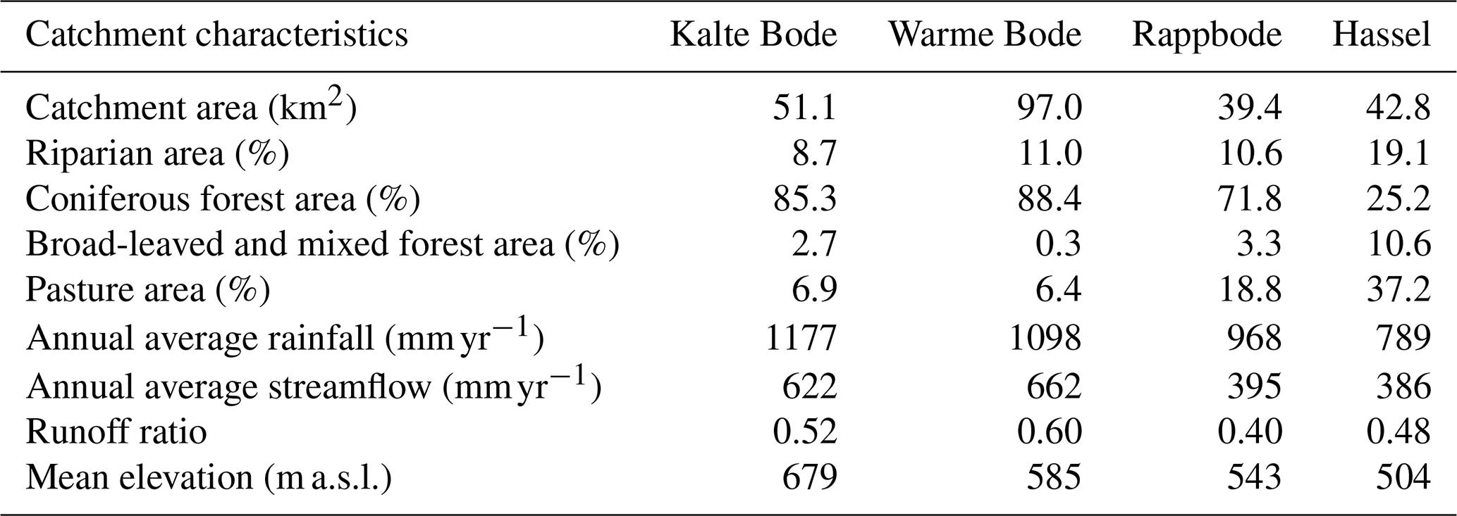
The area fraction of the riparian zone in the four catchments varies from 8.7 %–19.1 % (Table 1). These riparian zone proportions were calculated using a threshold value of the topographic wetness index (TWI) derived from a 25 m European Digital Elevation Model (EU-DEM). The riparian zone was defined as the combined area with TWI above a specific threshold. A TWI threshold was previously shown to be a robust measure of the riparian zones within catchments in Germany (Musolff et al., 2018). Here, the reference threshold (TWI≈6.8) was selected to match the areal extent of groundwater-dominated gley soils mapped in the Rappbode catchment (Werner et al., 2019) and then applied consistently across the four catchments. Because TWI-based delineation is a proxy for riparian extent rather than an exact hydropedological boundary, we evaluated the sensitivity of the main conclusions to this choice using an additional test in the Rappbode catchment (Sect. 4.4).

Gridded daily meteorological data (precipitation, air temperature, and potential evapotranspiration) from 2010–2018 over the study area were obtained from the German Weather Service. The land cover map was taken from the CORINE land cover map in 2018. Daily streamflow from 2010–2018 was provided by the federal state agency responsible for hydrological monitoring in the Harz Mountains. Weekly to biweekly stream DOC concentrations from grab samples collected between 2010 and 2018 were provided as part of the TERENO observatory (Zacharias et al., 2024) and the drinking water reservoir monitoring program (Kong et al., 2022).

2.3 Baseline calibration

In this study, we first calibrated the mHM (at a daily time step and 0.015625° resolution) models and then the DOC models as they rely on hydrological fluxes and storages from mHM as inputs. We calibrated the mHM models using observed streamflow at the respective catchment outlets with the Dynamically Dimensioned Search (DDS) Algorithm (Tolson and Shoemaker, 2007) as it is available within the mHM framework. We used the default parameter ranges in mHM (supporting information mhm_parameter.nml). DDS starts with a random initial parameter set and then updates the parameter set iteratively within the given ranges. The updated values depend on the previous best values (according to a certain objective function) and the iteration number. After each iteration (500 in total), the probability of a parameter being updated decreases. For each catchment, we repeated the DDS 30 times to get the respective 30 best hydrologic models (behavioural models) ranked based on the Kling–Gupta efficiency (KGE; Gupta et al., 2009) objective function value (Eq. 14) to account for parameter uncertainty.

With each of the 30 hydrologic models, we calibrated both models (lumped and landscape-explicit structures) using observed stream DOC concentrations at the respective catchment outlets by generating 100 000 random parameter sets using Latin Hypercube Sampling (LHS; Carnell, 2024; Stein, 1987) within selected parameter ranges based on our expert judgment and plausible values based on exploratory analyses of the model (supporting information doc_parameter.txt). This results in 30 (hydrological models) × 4 (number of catchments) × 2 (lumped and landscape-explicit models) ×100 000 model runs. This approach was used instead of DDS because it is simpler and has been demonstrated to be effective in finding behavioural parameter sets, especially when the number of parameters is small (Abbaspour, 2015). The best model (out of 100 000 runs) was selected based on the KGE metric (Eq. 14) for stream DOC simulation. For each catchment and each behavioural hydrological model, we searched for a corresponding behavioural DOC model using the aforementioned procedure. Therefore, we had 30 behavioural DOC models for each catchment.

The objective function used for calibrating the hydrological model (streamflow simulation) and DOC model (stream DOC simulation), i.e., the KGE, is expressed as follows:

$$\begin{array}{}\text{(14)}& \text{KGE}=\mathrm{1}-\sqrt{(r-\mathrm{1}{)}^{\mathrm{2}}+(\mathit{\alpha }-\mathrm{1}{)}^{\mathrm{2}}+(\mathit{\beta }-\mathrm{1}{)}^{\mathrm{2}}},\end{array}$$

where r is the linear correlation coefficient between simulated and observed values (streamflow or stream DOC concentration), α is the ratio between the standard deviation of the simulated and the standard deviation of the observed values (hereafter referred to as variability), and β is the ratio between the mean simulated and mean observed values (hereafter referred to as bias). In addition, we also showed different components of the KGE (correlation, variability, and bias) and the commonly used Nash–Sutcliffe Efficiency (NSE; Nash and Sutcliffe, 1970; Sect. S2) to assess the performance of the calibrated models. We selected KGE as our primary evaluation criterion as it balances between correlation, variability, and bias between observed and simulated data (Gupta et al., 2009). In contrast, NSE does not adequately account for variability (Gupta et al., 2009; Santos et al., 2018). We noted that calibration to stream DOC concentration is preferable to calibration to DOC load because DOC load is the product of streamflow and concentration. As a result, good performance for streamflow simulations can compensate for errors in simulated DOC concentrations, still producing acceptable load estimates. In contrast, calibrating to stream DOC concentration provides a more direct test of whether the model correctly represents the processes controlling DOC dynamics.

The hydrological and DOC models were calibrated for the period January 2015–June 2018 and validated for the period January 2010–December 2014. The calibration period was selected because DOC observations were more numerous in the Kalte Bode and Warme Bode catchments than during the validation period (Table S1 in the Supplement), allowing the calibration to be better constrained and to cover a wider range of stream DOC dynamics. The warm-up period was set to January 2000–December 2009 because a long hydrological time series is required to avoid the effect of initial conditions (e.g., initial SOC, or DOC in different model landscape units) on simulated results.

2.4 Constrained calibration

Under the constrained calibration, we calibrated the lumped and landscape-explicit model structures using the following constraints, and behavioural simulations were defined as those that satisfied all constraints and had the highest KGE for stream DOC concentration simulation.

• Constraint 1: the simulated average groundwater DOC concentration during the calibration period (January 2015–June 2018) should be within the range of [0.25–2.66] mg L⁻¹. This is based on the observed groundwater DOC concentrations in six springs (median 0.5 mg L⁻¹ and 90 % of the values are between 0.25 and 2.66 mg L⁻¹; LHW, 2026) within and near our study areas. In addition, observed DOC concentrations in groundwater in many other catchments worldwide are also low (median value of 1.2 mg L⁻¹ with ca. 84 % of the groundwater DOC samples below 5 mg L⁻¹; McDonough et al., 2020).

• Constraint 2: The simulated average DOC concentration in the outflows from the upland compartment during the calibration period should be less than half of that in the riparian zone (C_UL<0.5C_RZ). This constraint is based on our understanding of the DOC transport processes. By that, we acknowledge that most water from the upland has undergone an infiltration into the mineral layers of the soils before laterally entering the riparian compartment. The passage through the mineral soil will significantly reduce DOC concentrations due to adsorption, as mentioned in the introduction section (Kalbitz et al., 2000; Kothawala et al., 2012; Ledesma et al., 2018a).

All other settings for the calibration were identical to the baseline calibration, including using the same initial parameter range. The first constraint regarding groundwater concentration was applied to both model structures (lumped and landscape-explicit). In both structures, the groundwater compartment is located below the active soil layers, and its DOC concentration is primarily shaped by mineral interactions and long residence times rather than the spatial resolution of the recharge source. Thus, we consider the groundwater compartment to be effectively equivalent in both model structures. The second constraint was applied only to the landscape-explicit structure, as the lumped model structure does not separate between the upland and the riparian zone. In addition, we imposed an additional constraint (constraint 3) on the soil moisture factor affecting C transformation in the upland of the landscape-explicit model structure, whereby its value should be lower than that in the riparian zone ($k_{x\to y,\text{UL}}<k_{x\to y,\text{RZ}}$; Eqs. 1–2). This condition is based on the fact that riparian zones are wetter than upland areas given their location in the catchment in high TWI zones. Because the interaction between several model parameters that affect the soil moisture factor (e.g., field capacity, SMD_max, Eq. 2) can lead to unrealistic soil moisture factors, we needed to apply this condition to account for the physical difference between the two compartments.

The technical implementation of the constrained calibration process was as follows. First, we conducted 100 000 runs using the DOC model with parameter sets generated through Latin Hypercube Sampling (LHS) as described in Sect. 2.3, and we saved the parameter set, KGE value, average DOC concentrations in the upland, riparian zone, and groundwater, as well as the soil moisture factor in both the upland and riparian zones to reduce the model running time. Next, we applied the aforementioned constraints and selected the parameter set with the highest KGE. Finally, we reran the model with the best parameter set and extracted detailed outputs.

2.5 Scenario simulations

We performed a scenario simulation exercise with the aim of evaluating the credibility of lumped and landscape-explicit model structures calibrated with different constraints. We tested whether the lumped and landscape-explicit model structures could simulate stream DOC concentrations within a realistic range under a structural stress test where boundary conditions were changed. Specifically, we reran the models from the baseline and constrained calibration methods with an increase of C input of 5 $\mathrm{kg}{\mathrm{ha}}^{-\mathrm{1}}{\mathrm{d}}^{-\mathrm{1}}$ in the upland starting in 2015 (3 years of modelling under increased inputs). The initial range for calibration is [3, 12] $\mathrm{kg}{\mathrm{ha}}^{-\mathrm{1}}{\mathrm{d}}^{-\mathrm{1}}$ and therefore, C input in the scenario simulation could be from 8–17 $\mathrm{kg}{\mathrm{ha}}^{-\mathrm{1}}{\mathrm{d}}^{-\mathrm{1}}$, depending on the behavioural models found in the baseline and constrained calibration.

Results from previous studies could provide context for evaluating the results of this exercise. For example, Musolff et al. (2024) suggested that an increase in C availability in the upland (e.g., from forest dieback) will not lead to a significant increase in stream DOC concentrations due to the lack of direct hydrological connectivity. This can be attributed to a lack of hydrological connection of the upper upland soil layers with the stream, whereby a significant proportion of the increased C availability is processed in the upland soils and returned to the atmosphere as CO₂, while the rest of the DOC will be adsorbed in deeper mineral soil layers as the water percolates deeper into the groundwater (Musolff et al., 2024; Mikkelson et al., 2013; Kalbitz et al., 2000). Thus, we expected only minor changes in stream DOC concentrations under our scenario simulation exercise. We note that changes in DOC inputs are typically associated with changes in hydrological conditions. However, no changes were made to the hydrological simulations in this experiment, as the objective was to isolate the effect of C inputs on stream DOC responses and enable a clearer assessment of their influence.

Technically, the increased C input was represented in the model as an increase in root breakdown (RB) rate. The implementation of this scenario in the landscape-explicit model structure is straightforward as we have the upland and riparian zone explicitly represented. In the lumped model structure, this amount of C input increase was weighted by the areal fraction of the upland and was applied over the whole catchment.

3 Results

3.1 Hydrologic simulation

Visual assessment of the results shows that the seasonality of streamflow, low in summer (June–August) and fall (September to November), high in winter (December–February) and spring (March to May), from all catchments was well captured by the models (Figs. 3 and Fig. S2a). There was no systematic under- or over-estimation of high flows across all catchments or low flows in the Kalte Bode and Warme Bode catchments (Figs. 3a and S3). However, low flows were systematically overestimated in the Rappbode and Hassel catchment (Fig. S3b). The simulated average yearly hydrological fluxes show that Warme Bode, Rappbode, and Hassel have the highest outflow (as a percentage of streamflow) from the upland (or the full hillslope when referring to the lumped model structure) (median values>80 %) while that of the Kalte Bode is lower (median value ∼60 %) (Fig. S3). The average annual groundwater discharge from the groundwater compartment in the Kalte Bode (median value ∼35 %) is much higher than that of the Warme Bode, Rappbode, and Hassel (median values: ∼10 % to ∼15 %) (Fig. S3) due to the presence of granite bedrocks and Leptosols, creating higher groundwater recharge and flow. In both model structures, the amount of water discharge from the groundwater compartment is the same (Fig. 1). However, in the landscape-explicit model structure, between 10 % (Warme Bode) and 35 % (Hassel) of the groundwater discharge flows to the riparian zone before flowing to the stream.

Figure 3 (a) Time series of observed and simulated streamflow and (b) the model performance (KGE) of 30 behavioural streamflow simulations (the dots in the boxplots are the means). The solid lines and shaded areas (in blue) represent the medians and simulated ranges of these 30 streamflow simulations. Simulated streamflow from lumped and landscape-explicit model structures is identical; the differences between lumped and landscape-explicit model structures are the internal hydrological fluxes (Sect. S1).

Across all catchments, streamflow simulation in the calibration period is generally better than in the validation period: the mean KGEs of the behavioural models for the calibration period are significantly higher (p-value < 0.05; t-test) than those of the validation period. Yet, the model performances for streamflow simulation of the Warme Bode and Rappbode are comparable (mean KGEs of both calibration and validation periods are higher than 0.91 and 0.88, respectively) while those for the Kalte Bode and Hassel are slightly lower for the respective periods (mean KGEs of the behavioural models for the calibration and validation periods are 0.87 and 0.66 (Kalte Bode) and 0.77 and 0.68 (Hassel), respectively). The model performance for streamflow simulation is acceptable considering that all behavioural models achieve KGE>0.59 (Knoben et al., 2019). The components of the KGE, i.e., correlation, variability, and bias, and NSE (Figs. S5–S8) show similar patterns to those of KGE for streamflow simulation. It is also seen that, depending on the catchment, the contribution of each component of the KGE to its overall value (represented by its deviation from 1) differs. While these components are close to 1 for the Warme Bode and Rappbode, they deviate more substantially (within a range of 0.2) from 1 for the Kalte Bode and Hassel (Figs. S6–S8).

3.2 Stream DOC concentration dynamics under baseline calibration of the lumped versus landscape-explicit model structure

The simulated stream DOC concentration from the two model structures in the baseline calibration partly differ from each other (Fig. 4a and b, upper panel). For example, in the Kalte Bode and Warme Bode, the lumped model structure yields higher simulated stream DOC concentration ranges than the landscape-explicit model structure. However, both lumped and landscape-explicit model structures tend to miss major high-concentration events that have been observed in the Kalte Bode and Warme Bode catchments. Here, the maximum simulated stream DOC concentrations from the lumped model structure could be as high as 32 mg L⁻¹, while those in the landscape-explicit model structure are around 10 mg L⁻¹. In Rappbode and Hassel catchments, both model structures show similar simulated stream DOC (around 2–10 mg L⁻¹) and seasonal dynamics (high in summer and fall, low in winter and spring), which also resemble the observed data (Fig. S2b and c).

Figure 4 (a, b) Time series of observed and simulated stream DOC concentrations and (c, d) the model performance of 30 behavioural DOC simulations from (a, c) the lumped and (b, d) the landscape-explicit model structures during the calibration and validation of the baseline calibration. The solid lines and shaded areas (in blue) represent the medians and simulated ranges of these behavioural models. The dots in the boxplots are the means.

The landscape-explicit model structure does not always have a higher model performance (higher median KGE) than the lumped model structure (Fig. 4c and d, lower panel). In the Rappbode catchment, the lumped model structure (median KGE>0.60) outperforms the landscape-explicit model structure (median KGE<0.50) for both calibration and validation periods. However, both model structures show a comparable model performance for the Hassel catchment with a median KGE of about 0.63. In the Kalte Bode catchment, the landscape-explicit model structure has a higher median KGE for the calibration, but a lower median KGE for the validation than the lumped model structure. The opposite is true for the Warme Bode catchment, where both model structures show the lowest median KGEs among the four catchments. We note that the ranking of the model performance among catchments and periods is sensitive to the performance metrics. More specifically, the NSE, correlation, variability, and bias (Figs. S6–S8) do not show the same trend across the four catchments for the calibration and validation periods as that of the KGE (Fig. 4). Results also show that the contribution of different KGE components to its overall value differs (Figs. S6–S8).

3.3 Effect of constraints on stream DOC and model performance

The simulated stream DOC concentrations with the lumped model structure under the constrained calibration are in general lower than those under the baseline calibration and observed data across all catchments (Figs. 5a and S2b). In contrast, within the landscape-explicit model structure, there are only minor differences between the baseline and constrained calibrations at both daily (Fig. 5b) and seasonal timescales (Fig. S2b and c). For example, in the Warme Bode during winter and spring, the interquartile ranges of the simulated stream DOC concentrations using the landscape-explicit model structure under the constrained calibration are slightly wider than those under the baseline calibration (Fig. S2c).

Figure 5 (a, b) Observed and simulated stream DOC concentration from the lumped and the landscape-explicit model structures under the baseline (blue) and constrained (grey) calibrations, along with the model performance (c, d) for both calibration and validation periods together instead of separating the results by calibration and validation periods. Simulated results were taken from 30 behavioural DOC simulations. The dots in the boxplots are the means.

With the lumped model structure and across all four catchments, the model performance (mean KGEs) for stream DOC simulation under the constrained calibration decreases significantly (p-value < 0.05) compared to that under the baseline calibration (Fig. 5c). The magnitude of reduction in the model performance varies among catchments and models with an overall average decrease in the KGE of 0.14. In contrast to the lumped model structure, with the landscape-explicit model structure, the model performance for stream DOC simulation under the constrained calibration shows only a negligible (KGE decrease of 0.01 on average at Kalte Bode, Warme Bode, and Hassel, p-value < 0.05) or minor (KGE decrease of 0.08 on average at Rappbode, p-value < 0.05; see Fig. 5d) decrease. The NSE (except the Warme Bode catchment), variability, and bias also show a decrease in the model performance under the constrained calibration with the lumped model structure (Fig. S9a). However, the correlations under the baseline and constrained calibration with the lumped model structure are comparable. With the landscape-explicit model structure, the NSE, correlation, variability, and bias under the constrained and baseline calibrations are comparable across most of the catchments (Fig. S9b).

3.4 Effects of constraints on the number of feasible simulations and parameter distribution

It is seen that the effect of each constraint depends on the model structure, catchment, and the type of constraint applied (Table 2). For the same constraint (e.g., constraint 1 for groundwater DOC concentration), a smaller percentage of satisfied simulations with the landscape-explicit model than with the lumped model indicates greater uncertainty in the simulated internal DOC dynamics of the more complex model structure. Among the three constraints applied on the landscape-explicit model structure, constraint 2, which represents the relationship between upland and riparian-zone DOC concentrations, is the most restrictive. This highlights the importance of realistically representing spatial DOC gradients between upland and riparian zones. Most parameter distributions change little after applying the constraints (Figs. S10 and S11). However, a few parameters show substantial shifts from their initial distributions, particularly those controlling the rate of SOC to DOC conversion in the upland or hillslope.

Table 2 Percentage of simulations satisfying each individual constraint and combinations of constraints among the 30×100 000 simulations performed for each catchment using randomly generated parameter sets. Constraints 1, 2, and 3 correspond to groundwater DOC concentration ($\mathrm{0.25}<\text{CGW}<\mathrm{2.66}\mathrm{mg}{\mathrm{L}}^{-\mathrm{1}}$), the relationship between upland and riparian zone DOC concentrations (C_UL<0.5C_RZ), and the relationship between C transformation rate in the upland and riparian zone ($k_{x\to y,\text{UL}}<k_{x\to y,\text{RZ}}$), respectively (Sect. 2.4).

3.5 Effects of constraints on internal DOC dynamics

Under the baseline calibration, most of the simulated groundwater concentrations with the lumped model structure are above the threshold level (2.66 mg L⁻¹) defined in the constrained calibration (Fig. 6a). Under the constrained calibration, the maximum simulated groundwater concentrations with the lumped model structure are slightly above 2.66 mg L⁻¹ (as the constraint was imposed on the average value; Fig. 6b). Moreover, in all catchments, the simulated hillslope DOC concentrations under the constrained calibration are lower than those under the baseline calibration, especially in the Kalte Bode and Hassel (Fig. 6 and b).

Figure 6 Internal DOC concentrations in different landscape units from the lumped model structures under (a) the baseline and (b) constrained calibrations.

With the landscape-explicit model structure for the Kalte Bode and Warme Bode, there are minor differences in the internal DOC concentrations under the baseline (Fig. 7a) and constrained (Fig. 7b) calibration. In the Rappbode and Hassel catchment, however, there are clear differences in the groundwater and upland DOC concentrations under the baseline and constrained calibration. For example, the maximum simulated groundwater DOC concentrations in the Rappbode and Hassel with the landscape-explicit model structure and under the baseline calibration reach 9 mg L⁻¹ while those under the constrained calibration are slightly above 2.66 mg L⁻¹. The maximum simulated upland DOC concentrations in the Rappbode and Hassel with the landscape-explicit model structure under the constrained calibration significantly decrease compared with those under the baseline calibration (e.g., Hassel: from above 15.0 mg L⁻¹ to less than 5.4 mg L⁻¹).

Figure 7 Internal DOC concentrations in different landscape units from the landscape-explicit model structures under (a) the baseline and (b) constrained calibrations.

3.6 Changes in stream DOC concentrations under scenario simulations

In this section, we report results from the Hassel catchment (Fig. 8) as an example. Results obtained from the three remaining catchments (Fig. S12) are similar to those from the Hassel catchment. With the lumped model structure (Fig. 8a), increasing C input in the upland soils would significantly increase (p-value < 0.05) stream DOC regardless of the calibration approach (mean DOC concentration increases from 5.1–7.0 mg L⁻¹ and from 3.3–5.2 mg L⁻¹ when using the baseline and constrained calibrated models, respectively). By contrast, using the landscape-explicit model structure (Fig. 8b), the changes in stream DOC concentration are lower than 0.1 mg L⁻¹ and therefore negligible when increasing C input in both calibration approaches.

Figure 8 Simulated stream DOC concentrations in the Hassel catchment with increasing C input by 5 kg ha⁻¹ for the period 2015–2018 (a) in the hillslope of the lumped model structure, and (b) in the upland of the landscape-explicit model structure.

When increasing C input, results show that there are negligible changes ($<\mathrm{0.1}\mathrm{mg}{\mathrm{L}}^{-\mathrm{1}}$) in the mean groundwater DOC concentrations across all model structures and calibration methods (results were not shown here). However, there are significant (p-value < 0.05) increases in the mean hillslope DOC concentration with the lumped model structure that were calibrated under the baseline calibration (an increase of 2.7 mg L⁻¹ or 45 %) and the constrained calibration (an increase of 2.6 mg L⁻¹ or 70 %). With the landscape-explicit model structures, we found increases of 1.3 mg L⁻¹ (59 %) and 1.1 mg L⁻¹ (83 %) in the upland DOC concentrations with the models calibrated under the baseline and constrained calibrations, respectively. There are negligible changes ($<\mathrm{0.1}\mathrm{mg}{\mathrm{L}}^{-\mathrm{1}}$) in riparian DOC concentrations with the landscape-explicit model structures across all calibration methods.

4 Discussion

4.1 The right results for the wrong reasons? DOC dynamics under baseline calibration

Application of the lumped and landscape-explicit model structures under the baseline calibration shows that both structures can give a satisfactory model performance for stream DOC concentrations (Fig. 4). This is in line with previous studies, in which both model structures were successfully applied for stream DOC simulation (Birkel et al., 2014, 2017; Strohmenger et al., 2021). However, not all of the simulated DOC concentrations in the internal model units (e.g., hillslope, upland, and groundwater) from lumped and landscape-explicit model structures fit our process understanding and observations (Sect. 3.3). In fact, with the lumped model structure, most of the behavioural models under the baseline calibration do not meet our understanding regarding low groundwater DOC concentrations. More specifically, the lumped model needs implausibly high groundwater DOC concentrations to compensate for the low DOC concentration from the hillslope during high flow periods in order to match observed stream DOC concentrations. With the landscape-explicit model structure, 53 % of behavioural models under the baseline calibrations meet all of our constraints across all four catchments (Sect. 2.4). However, in contrast to the lumped model, the landscape-specific model structure maintains a good performance after constraining the groundwater concentrations to the observed range and the upland concentration to match our understanding of the different compartments. Examining internal DOC concentrations has often been neglected in catchment DOC models, either due to data availability or because these are not the variables of interest. Using models that inconsistently simulate internal DOC dynamics could lead to a false interpretation and potentially to wrong management decisions. Here, together with other water quality studies (i.e., Fohrer et al., 2022; Lutz et al., 2022), we emphasize the need for also evaluating concentrations and fluxes in and between internal model compartments.

Thus, our results show that stream DOC concentration alone is not sufficient to constrain either lumped or landscape-explicit model structures in terms of internal DOC concentrations and fluxes. The interplay between different parameters affecting DOC production, together with the added complexity of having those parameters acting in different model compartments (i.e., upland, groundwater, and riparian zone) result in a myriad of model simulations that are able to reproduce stream DOC dynamics, but not necessarily able to represent landscape-internal DOC dynamics. With more complex model structures, there is a higher degree of freedom and a higher uncertainty in model parameterization, leading to higher uncertainty in the internal DOC dynamics. For example, wider simulated groundwater DOC concentration ranges were found from the landscape-explicit model structure than from the lumped model structure in the baseline calibration (Figs. 6 and 7). This is because the amount of groundwater that flows directly to the stream in the landscape-explicit model structure is less than that in the lumped model structure (Fig. 1 and Sect. 3.1), making the information content of observed stream DOC concentration ineffective for constraining groundwater DOC concentration. Similarly, there is also a high uncertainty in the upland DOC concentration from the baseline calibration, as DOC in the upland does not flow directly into the stream.

On the other hand, the landscape-explicit model structure enforces a conceptual understanding that also constrains, to a certain extent, the degree of freedom. More specifically, the introduction of the riparian zone compartment that upland water needs to pass, limits the instream DOC concentration range. Since the riparian zone has a constantly high soil moisture, the concentration range is mainly dictated by soil temperature (see Sect. 2.1) while contributions from upland are buffered by mixing with the riparian DOC mass. Soil moisture variations in the hillslope allow for a higher DOC concentration range that can be transferred to the stream. However, we argue that this direct connectivity is limited or non-existent in our catchments and therefore gives the right answer (peak concentrations in stream DOC are met) for the wrong reason (peak DOC comes from the dryer upland or hillslope compartment) (Musolff et al., 2024, Ledesma et al., 2018a, Ledesma et al., 2025). The lumped model therefore has greater freedom to reproduce stream DOC peaks and, in some cases, particularly Rappbode, shows better agreement with observed stream DOC according to KGE (Fig. 4). However, this apparent improvement comes at the cost of implausible internal DOC concentrations and fluxes, suggesting that the right stream DOC response is obtained for the wrong internal reason.

Indeed, there is evidence from the Rappbode catchment that riparian zone DOC concentrations can be higher (observed up to 16 mg L⁻¹, Ledesma et al., 2025) than modelled here (range 2.5–9 mg L⁻¹, Fig. 7). Here, future model refinements may allow for a higher concentration range in the riparian zone, for example, by accounting for vertical heterogeneity in water flows and the associated depth-dependent DOC mobilization from riparian zones as described by Seibert et al. (2009) or Ledesma et al. (2018b).

The finding that instream DOC is not sufficient to constrain the DOC concentrations in other model compartments is supported by similar results from previous studies, which focused on other water quality variables. Nguyen et al. (2022) found considerable uncertainty in the internal modelled results (i.e., soil nitrogen storage, groundwater nitrate concentration) when their models were only calibrated to the integrated signal (i.e., stream nitrate concentration) at the catchment outlet. They emphasized the need for more data to better constrain the model. For DOC modelling, we demonstrated that incorporating data from groundwater DOC concentrations or relative DOC concentration understanding from different landscape units (e.g., upland and riparian zones) could help to better constrain internal model states, which would otherwise be highly uncertain and likely implausible when calibrated solely based on instream DOC concentrations.

4.2 The value of a landscape-explicit structure and a constrained calibration

The results of this study demonstrate that under the constrained calibration, model performance in terms of stream DOC concentration might be compromised as a result of the applied constraints. When additional constraints are introduced, the solution space becomes more limited (Salmon-Monviola et al., 2025), potentially leading to a lower number of parameter sets able to satisfactorily reproduce stream dynamics. However, the simulated internal DOC concentrations under the constrained calibration are more consistent with our understanding and observed data (Sect. 3.3), highlighting the value of constraining the model.

The value of the landscape-explicit structure was revealed in our scenario simulations. With the lumped model structure, we could only impose the constraint on the simulated groundwater DOC concentrations, and the contribution of groundwater DOC to stream DOC is minor compared to that of the hillslope due to relatively low groundwater flow and DOC concentration (Figs. S3 and 6). Thus, the scenario in which we increased C inputs in the lumped structure led to a significant increase in simulated stream DOC concentrations, which does not match our expectation based on observations (Musolff et al., 2024). By contrast, with the landscape-explicit model structure calibrated under the baseline and constrained calibrations, the majority of stream DOC originates in the riparian zone. Therefore, both calibration routines show negligible changes in stream DOC concentration during the scenario simulation case, which matches our expectations based on our observations in the Rappbode catchment, where an increased C input in the upland led to minor changes in the stream DOC concentrations (Musolff et al., 2024).

4.3 Implications for model evaluation and model structure selection

The results of our study indicate that a DOC model evaluated solely on its ability to simulate stream DOC concentrations may not serve as a robust prognostic tool under changing conditions. A lumped model structure might outperform a landscape-explicit model structure for stream DOC concentration simulation (e.g., Fig. 4 – Rappbode catchment), but it is likely that the lumped model structure cannot be used for scenario exploration (Sect. 3.4). We argue for using only model structures that can be justified (Beven and Freer, 2001). In line with the arguments presented by Beven and Freer (2001), this justification should be based on observations or qualitative understanding of the catchment processes as demonstrated in this study, even when the overall performance of the justifiable models might be lower.

With more complex models, e.g., SWAT-Carbon (Zhang et al., 2013), INCA-C (Futter et al., 2007), HYPE (Pers et al., 2016); BioRT-Flux-PIHM (Wen et al., 2020), the available data may be insufficient to constrain all model parameters. Still, the models can exhibit substantial equifinality (i.e., multiple parameter sets may produce equally acceptable simulations), resulting in a wide range of potential solutions, some of which may be unrealistic. This is consistent with our experience, which indicates that although a landscape-explicit model represents a structural advancement, it may not always produce internal DOC dynamics consistent with the imposed observations and process-based constraints. Therefore, we recommend that modelers critically evaluate which model outputs can be used, prioritizing those that have been evaluated by direct observations or corroborated by expert knowledge.

4.4 Limitations

The calibration constraints implemented in this study were restricted to those that could be supported by available observational data and by our perceptual model of relative DOC concentrations among landscape units. Additional constraints, e.g., the relative magnitude of DOC concentrations in the upland, groundwater, and riparian zone compared to stream DOC concentration during different flow conditions could be used if such information is available (e.g., Wen et al., 2020). We did not conduct a separate evaluation of the simulated stream DOC under different flow conditions. Our analysis focused on whether the alternative model structures reproduced overall stream DOC dynamics and whether their internal DOC dynamics were consistent with available observations and process understanding. An extensive evaluation of model performance under different flow conditions is required if the focus is on event DOC dynamics and understanding the model's strengths and limitations under such conditions. In addition, we found that the extent of the riparian zone is sensitive to the defined TWI threshold, highlighting uncertainty in the TWI-based delineation. In the Rappbode catchment, changing the riparian extent by ±25 % resulted in a wider range of model performance for stream DOC simulation, while the main findings remained unchanged (Sect. S3). Because this sensitivity analysis was conducted only for Rappbode catchment, its results should not be interpreted as demonstrating robustness to riparian-zone delineation across all four catchments. However, given the broadly similar catchment characteristics and the consistent modelling framework applied across sites, a comparable response might be expected in the other catchments.

Furthermore, a more vertically refined representation of the riparian zone, e.g., through multiple soil layers, could account for depth-dependent DOC concentrations and for changes in the riparian source layer contributing to stream DOC under variable flow conditions. This could potentially improve the simulation of high DOC concentrations, especially for the Kalte Bode and Warme Bode catchments (Fig. 5b), as well as the representation of groundwater DOC concentrations. Additional stream DOC observations, particularly during high DOC concentration events, would also help to better characterize DOC export across the full range of hydrological and biogeochemical conditions. This is especially relevant for Warme Bode, where observed stream DOC concentrations span a wider range than others (Fig. 4). Under such conditions, sparse weekly or biweekly sampling may miss short-lived DOC peaks and therefore provide limited information for evaluating event-scale model behaviour. High-frequency DOC measurements or suitable optical proxies, would help to constrain these dynamics more directly and could improve the representation of high-DOC events in the model.

Our model was based on the mass balance of C for each C pool and model compartment. In other words, all C influxes and outfluxes associated with each C pool (Fig. 1c) were explicitly represented in the model. However, only the DOC fluxes were constrained through calibration against observed stream DOC concentrations. Other simulated C fluxes, such as the conversion of SOC to DIC and DOC to DIC, as well as the SOC and DIC storage estimates, were not directly constrained by observations. These fluxes and storages should therefore be interpreted with caution. Future studies could evaluate them more directly as additional observational data on C pools and transformation fluxes become available.

5 Summary and Conclusions

Elevated DOC concentrations are a major concern for ecosystems and drinking water supply from surface water reservoirs. Robust modelling tools for predicting terrestrial DOC export to the aquatic system are highly relevant. Data-driven studies revealed variable functioning of different landscape units (upland, riparian zone, and groundwater) in catchment DOC mobilization and export. Both lumped and landscape-explicit (separating upland and riparian zone) model structures are in use. They are generally calibrated to observed stream DOC concentrations, while the landscape-internal DOC dynamics do not receive sufficient attention. Here, we developed a flexible model with a lumped and a landscape-explicit conceptualization for four headwater catchments in the Harz Mountains, Germany. We evaluated the simulated internal DOC concentrations when the model was calibrated using stream DOC concentration alone (baseline calibration) versus using additional constraints based on “soft” data and our perceptual model of relative DOC concentrations among landscape units (constrained calibration). We further conducted a scenario simulation exercise in which we increased carbon input to the upland to evaluate the simulated response of stream DOC concentration under different model structures. The key findings from our study are listed below.

• Under the baseline calibration, both lumped and landscape-explicit model structures can reasonably represent stream DOC concentration dynamics, with none consistently outperforming the other across catchments and evaluation metrics. However, the simulated DOC concentrations in groundwater for both model structures were significantly higher than those from observations, indicating unrealistic internal DOC dynamics.

• The constrained calibration slightly reduces model performance for stream DOC concentration simulation for the landscape-explicit model structure while producing internal DOC dynamics consistent with the imposed observational and process-based constraints. In contrast, the performance of the lumped model structure is significantly reduced under the constrained calibration.

• For evaluating the effectiveness of spatial management on stream DOC (e.g., changes that do not occur homogeneously over the entire catchment, such as increasing C input in the upland in this study), a landscape-explicit model structure provides results consistent with observation-based analyses, while a lumped structure does not.

We call for a careful evaluation of the physical realism of the DOC processes in the internal model compartments of other DOC models. This is crucial, particularly when management decisions should be robust, also under changing boundary conditions.