Spectral analysis of groundwater level time series for robust estimation of aquifer response times

Groundwater resources represent Germany's most important source of freshwater but they are increasingly under pressure. Climate change, societal developments, and rising abstraction rates are impacting subsurface storage in ways that are currently difficult to predict, affecting both the quantity and quality of groundwater. To ensure sustainable groundwater management, it is crucial to evaluate the intrinsic and spatially variable vulnerability of groundwater systems, especially to prepare for the effects of hydrological extremes. In this context, the groundwater response time, generally defined as the timescale over which a groundwater system responds or adjusts to changes in external or internal conditions and derived here as the characteristic timescale of the aquifer's low-pass filtering behavior, serves as a valuable indicator for vulnerability assessments. Unlike traditional methods, we propose estimating response times through spectral analysis of groundwater level data. Time series from around 200 selected observation wells across Bavaria in Southern Germany were processed and transformed into the spectral domain. Corresponding recharge time series were extracted from high-resolution hydrological model outputs. By integrating these data with hydrogeomorphic information, we fitted a semi-analytical model to the groundwater level spectra to obtain aquifer response times. The semi-analytical solution for the spectral domain accurately reproduced the majority of observed groundwater level spectra. Half of the estimated response times fall between 30 and 100 d. Significant correlation were found between the response time and the depth of the groundwater table. Groundwater systems exhibiting longer response times are interpreted as more resilient to drought conditions and therefore potentially better suited for groundwater abstraction than aquifers with shorter response times.

1 Introduction

In the last decade, Central Europe experienced a series of hot and dry periods resulting in severe droughts such as the extraordinary drought period in 2018–2020. These conditions greatly affected groundwater systems, as increased abstraction for households, industry, and agriculture set additional pressure on water resources (Luetkemeier et al., 2022; Wanders and Wada, 2015). Furthermore, during the winter season, droughts were accompanied by reduced groundwater recharge, leading to lower replenishment of groundwater systems compared to normal conditions. Jasechko et al. (2024) analyzed more than 100 000 data sets for more than 1600 aquifer systems worldwide and showed that rapid groundwater level declines (more than 0.5 m yr⁻¹) are widespread in the twenty-first century, especially in dry regions with extensive cropland areas. In summary, both reduced recharge and excessive water withdrawals contribute to declining groundwater levels, which in turn leads to a decrease in baseflow that sustains river systems.

Beside evidence from past data analysis, model-based hydrometeorological projections state that the risks of droughts-in particular longer lasting and stronger droughts-will continue to increase in Europe (Ciscar et al., 2019; European Commission, 2021; IPCC, 2023). Coupled climate-hydrological model simulations by Samaniego et al. (2018) project more frequent soil moisture droughts across Europe, along with a 40±24 % increase in drought-affected areas, if global warming reaches 3 K. The consequences on groundwater recharge and thus groundwater systems, however, are difficult to estimate and subject of great uncertainty-at least in Central Europe (Kumar et al., 2025).

A central question therefore is: how long are groundwater systems capable of buffering periods of strongly reduced groundwater recharge or strongly increased groundwater withdraws? An essential property describing the capacity of groundwater systems to buffer and moderate fluctuations in recharge or pumping stresses is the groundwater response time (also known as aquifer response time or characteristic time). Generally speaking, this parameter quantifies the time required for the groundwater system to relax after or respond to changes in recharge rates or excessive abstraction (Jazaei, 2017; Carr and Simpson, 2018; Houben et al., 2022) which is derived here from the characteristic timescale of the aquifer's low-pass filtering behavior.

Various methods exist to estimate groundwater response times, based on time series of groundwater levels or baseflow. A common approach is to measure the lag time between a specific event such as a drought during which recharge to the system ceases and the response of the groundwater level. The recession time of baseflow under such drought situations or the recovery time of baseflow after the drought has ended is then considered to be the response time of the contributing aquifer systems (Brutsaert, 2008). Lee and Ajami (2023) analyzed data of baseflow data from 358 anthropogenically unaffected catchments across the United States to characterize droughts and recovery properties of baseflow. The catchments they investigated showed baseflow droughts that last between 9–104 months, which is longer than the corresponding precipitation droughts. A challenge in applying this approach is accurately defining the start and end of a dry period, as these depend on the characteristics of each specific event.

Changnon (1987) developed a practical framework for detecting the onset, severity, and termination of droughts by monitoring precipitation, soil-moisture levels, shallow groundwater levels, and streamflow. In the groundwater system, a drought is classified as moderate when groundwater levels fall more than 30 % below the long-term mean for at least three consecutive months, and as severe when the decline exceeds 55 % for at least twelve months. Identifying the end of a drought is more complex; it generally requires a rise in soil moisture accompanied by several months of excess precipitation.

Under the linear-reservoir approximation, the time needed for groundwater levels to drop below a drought-threshold is directly related to the recession constant. Hameed et al. (2023) applied this concept by analysing individual base-flow events from 1990–2019, extracting them from streamflow records with complementary precipitation data, and estimating the corresponding recession constants. Although the drought definition is straightforward in theory, inverse estimation of response times from time series data introduces uncertainties that can cause variations in the derived recession constants, even for a single hydrograph. This might also explain why Hameed et al. (2023) found large variations in recession constants for a single catchment using event-based recession analysis.

Lee and Ajami (2023) further emphasized that the onset of a baseflow drought should be viewed as a process rather than an instantaneous event. Because baseflow responds delayed and dampened to precipitation, they adopted the concept of an intermittent above-zero standardised baselow Index (SBI) during drought periods introduced by Parry et al. (2016).

Another approach is to consider groundwater systems as systems that continuously receive recharge driven by precipitation and also react to this continuously varying stimulus with fluctuating groundwater levels and temporarily varying baseflow. Within this context, response times are often estimated by correlating standardized groundwater level or baseflow data with standardized time series of precipitation accumulated for different periods. Following this approach, Hellwig and Stahl (2018) investigated past changes and potential future changes in baseflow for 338 headwater catchments across Germany. They presented baseflow response times that vary across Germany, ranging from a few months to several years. In addition, the resulting response times depend on the hydrogeological properties of the catchments. A limitation of using baseflow data, however, is that it describes the response of aquifer systems at the catchment level. The analogous analysis of groundwater level data allows to infer local groundwater response times. Boumaiza et al. (2021) found aquifer response times between one and three months in Saint-Honoré aquifer in Canada using a sliding cross-correlogram approach and Kumar et al. (2016) analyzed groundwater level data from the Danube and additional catchments in the Netherlands. Both, Kumar et al. (2016) and Boumaiza et al. (2021) observed that response times differ within a given aquifer and are influenced by the thickness of the vadose zone. Thicker vadose zones lead to longer response times. The latter result points to a limitation of this method: the response time estimates include the transit time of the pressure signal through the vadose zone. Therefore, they are not only reflecting the aquifer response times but also the response time of the whole coupled subsurface system.

While the vadose zone is a primary and potentially the dominant driver of hydrological signal filtering, as demonstrated by Tsypin et al. (2025) and Liesch and Wunsch (2019), the saturated aquifer independently functions as a low-pass filter governed by its intrinsic hydraulic properties: transmissivity T and storativity S. Although confined aquifers possess limited pore-space elasticity, resulting in low storativity, a concurrently low T can still yield significant characteristic response times.

Several theory-based approaches have evolved over recent decades (Gelhar and Wilson, 1974; Erskine and Papaioannou, 1997; de Rooij, 2012, 2013; Jazaei, 2017; Carr and Simpson, 2018). For example, dimensional analysis of the linearized Boussinesq equation (Bear, 1972; Freeze, 1979) demonstrates that a characteristic time scale of an aquifer is governed by a combination of three key parameters: a typical length L, the storativity S and the transmissivity T of an aquifer which relate as follows:

$$\begin{array}{}\text{(1)}& t_{\mathrm{c}}={\displaystyle \frac{L^{\mathrm{2}}S}{T}}\end{array}$$

Cuthbert et al. (2019) and colleagues applied this formula to estimate groundwater response times on a global scale. They used globally derived values for the relevant parameters and incorporated them into the formula. The result is a gridded map of groundwater response times, which typically range from several years to several hundred years. These results clearly contradicts results of much smaller response times presented by Kumar et al. (2016), Hellwig and Stahl (2018) and Houben et al. (2022) and for German catchments, Boumaiza et al. (2021) for Canadian aquifer systems, as well as our findings in this work.

Recently, Carr and Simpson (2018) developed a new method for calculating highly accurate estimates of response times for groundwater flow processes. The analysis is carried out using the linearized, one-dimensional Dupuit-Forchheimer model of saturated flow through a heterogeneous porous medium and is based on hydraulic head (i.e., hydrostatic pressure) measurements.

Alternatively, spectral approaches can be used to infer response times. Zhang and Schilling (2004, 2005), Zhang and Li (2006), Zhang and Yang (2010), Schilling and Zhang (2011), Liang and Zhang (2013, 2015), Zhang et al. (2022) and Pujades et al. (2023) investigated the spectral analysis method (SpA) based on semi-analytical solutions of groundwater flow equations for the frequency domain and analyzed various groundwater systems. Houben et al. (2022) demonstrated its capability to estimate aquifer parameters like response times, storativity as well as transmissivities from long groundwater time series in a virtual (numerical) aquifer and exemplarily applied the method to measured data from groundwater levels in central Germany. As an advantage, spectral methods yield response time estimates that reflect the system's overall dynamic behavior, since the full spectrum of frequencies is analyzed. This contrasts with recession constant analysis, which relies on identifying and analyzing individual events. A potential drawback of frequency domain approaches is that sufficiently long time series of groundwater data are required.

In this work, we apply the spectral analysis workflow (SpA) introduced by Houben et al. (2022) to groundwater level time series from 209 observation wells in Bavaria, Germany. We confirm and further demonstrate the robustness of the approach in determining groundwater response times from real data and provide thorough interpretation of the results.

The Methodology section outlines the theoretical foundations of spectral analysis, detailing a systematic workflow encompassing data preparation, pre-processing, and final parameter estimation. The Results section presents representative types of groundwater level spectra along with the corresponding estimates of aquifer response times. An in-depth Discussion addresses the uncertainties inherent in the analysis and explores the broader implications of the findings. Finally, concluding remarks are presented at the end of this work.

2 Methodology

2.1 Theoretical Background

Aquifers typically act as low-pass filters (Zhang and Schilling, 2004), i.e., they transform incoming signals, such as the recharge, into a signal with decreased (dampened) high frequency content above a specific cut-off frequency. This cut-off frequency is inversely related to the aquifer response time.

Spectral analyses relies on the Fourier transform of a temporal signal g(t) (e.g., measured groundwater levels over time). The Fourier transform is defined by the following equation:

$$\begin{array}{}\text{(2)}& \widehat{g}\left(\mathit{\omega }\right)=\underset{-\mathrm{\infty }}{\overset{\mathrm{\infty }}{\int }}g\left(t\right)e^{\mathrm{2}\mathit{\pi }i\mathit{\omega }t}\mathrm{d}t\end{array}$$

where $i=\sqrt{-\mathrm{1}}$ and ω is the frequency. $\widehat{g}\left(\mathit{\omega }\right)$ represents the frequency share of the original signal. The Fourier transform of the temporal autocorrelation function R_hh of the signal is the spectral density S_hh (in this work also referred to as spectrum)

$$\begin{array}{}\text{(3)}& S_{\mathrm{hh}}\left(\mathit{\omega }\right)=\underset{-\mathrm{\infty }}{\overset{\mathrm{\infty }}{\int }}{R}_{\mathrm{hh}}\left(\mathit{\tau }\right)e^{-\mathrm{2}\mathit{\pi }i\mathit{\omega }\mathit{\tau }}\mathrm{d}\mathit{\tau }\end{array}$$

where R_hh is assumed to be stationary in time and τ is the time. Based on this relation, Liang and Zhang (2013) developed a semi-analytical solution for a groundwater head spectrum of an 1D groundwater transect with homogeneous aquifer properties. Details of its derivation can be found in Liang and Zhang (2013) and Houben et al. (2022). The final equation reads:

$$\begin{array}{}\text{(4)}& {\displaystyle }\begin{array}{rl}{S}_{\mathrm{hh}}(x,\mathit{\omega })& ={\displaystyle \frac{\mathrm{16}}{{\mathit{\pi }}^{\mathrm{2}}{S}^{\mathrm{2}}}}\sum _{m=\mathrm{0}}^{\mathrm{\infty }}\sum _{n=\mathrm{0}}^{\mathrm{\infty }}{\displaystyle \frac{(-\mathrm{1}{)}^{m+n}{B}_m{B}_n{S}_{\mathrm{ww}}}{(\mathrm{2}{m}^{\mathrm{2}}+\mathrm{2}{n}^{\mathrm{2}}+\mathrm{2}m+\mathrm{2}n+\mathrm{1})}}\\ & \cdot {\displaystyle \frac{(\mathrm{2}m+\mathrm{1}{)}^{\mathrm{2}}}{(\mathrm{2}m+\mathrm{1}{)}^{\mathrm{4}}(\frac{\mathrm{4}}{{\mathit{\pi }}^{\mathrm{2}}}{t}_c{)}^{-\mathrm{2}}+{\mathit{\omega }}^{\mathrm{2}}}}\end{array}\text{(5)}& {\displaystyle }{B}_m={\displaystyle \frac{\cos \left[\right(\mathrm{2}m+\mathrm{1})\mathit{\pi }{x}^{\prime }/\mathrm{2}]}{(\mathrm{2}m+\mathrm{1})}},x^{\prime }={\displaystyle \frac{x}{L}}\end{array}$$

It relates the spectrum of groundwater level fluctuations S_hh at a certain location to the groundwater recharge spectrum S_ww. S is the storativity, x is the distance of the observation well (where time series are recorded) to the water divide and L is the aquifer length from the water divide to the river. Then, the response time t_c is given by

$$\begin{array}{}\text{(6)}& t_{\mathrm{c}}={\displaystyle \frac{L^{\mathrm{2}}S}{T}}\end{array}$$

t_c depends on the length L, the storativity S and the transmissivity T of the observed aquifer. It can range from a few weeks for small and highly conductive aquifers with low specific storage to several months or years for large aquifers with low transmissivities and higher storativities.

Since t_c is fitted to the power spectral density of the head and recharge signals, it is a phase-blind, frequency-domain descriptor of the aquifer's overall low-pass filtering strength. Consequently, it does not represent a directional lag time between the onset of a forcing event and the corresponding response (Kirchner et al., 2023), nor any asymmetry between the rise and recession limbs of that response as in Lee and Ajami (2023).

2.2 Data and Workflow

2.2.1 Study Area: Bavaria

Central for the analysis are long time series of groundwater level measurements at different locations and hydrogeological units. For this study, 298 groundwater observation wells from the monitoring network of the Bavarian State Office for the Environment (LfU) representing the upper groundwater stockwerk (groundwater table depth smaller than 100 m) were selected and the corresponding groundwater level time series were downloaded via the online service (Bayerisches Landesamt für Umwelt, 2022). The wells are distributed throughout the state and cover relevant hydrogeological units where groundwater abstraction takes place (Fig. 1a). The State of Bavaria is located in the south of Germany and its southern border is dominated by the up to 3000 m high Alpine Mountains with steep folded hard rocks with low groundwater yield. Northward the mountains transit into the wide and flat Molasse Basin, which is filled with hundreds of meters thick unconsolidated debris from the Alps, hosting most productive shallow aquifers. Similarly, Quaternary valley fillings constitute productive aquifers. In the central and northern parts of the state however, faulted blocks of Mesozoic lime-, dolo- and sandstones form the hilly landscape and host groundwater in medium productive and partly karstified aquifers. These areas are framed by lifted blocks of crystalline Paleozoic basement forming a few hundreds meters high mountain ranges. No groundwater observations exist there. Even if the time series are distributed all over the hydrogeological units, forming the upper groundwater stockwerk, the majority of observation wells are located in the Molasse Basin and Quaternary sediments surrounding the larger rivers draining from the Alps through glacier valleys towards the Danube River (Fig. 1a).

2.2.2 Time Series Preparation (Fig. 2a and b)

The majority of the groundwater time series cover at least 15–20 years of data with a few being 50 years long. All of them end at the beginning of 2019. Houben et al. (2022) demonstrated that time series should cover a time duration of at least ten times the expected characteristic time of the aquifer to obtain correct estimates of the power spectrum containing all frequencies with enough spectral power. Following this, time series with a length of less than 2 years were discarded. Finally 224 time series remained for the analysis.

The groundwater level time series had different sampling intervals and irregular lengths. Since spectral analyses requires equidistant time steps, the time series were interpolated to a daily time step. The derivation of the semi-analytical solution for the head spectrum assumes a stationary process, which was not always the case for the analyzed groundwater level time series. Roughly 25 % of the time series had severe jumps or inconsistencies in the recorded data due to changing sampling interval or other artifacts, thus these time series were screened and a representative and stationary period was selected for further processing.

First, the raw data was processed to obtain time series suitable for the analysis. In a first step, outliers were removed using the interquartile range $\text{IQR}=Q_{\mathrm{3}}-Q_{\mathrm{1}}$. The lower limit was determined as ${\lim }_{\mathrm{low}}=(Q_{\mathrm{1}}-\mathrm{1.5}\cdot \text{IQR})$ while the upper limit was defined as ${\lim }_{\mathrm{up}}=(Q_{\mathrm{3}}-\mathrm{1.75}\cdot \text{IQR})$. In a second step, the time series were interpolated to ensure equidistant time steps of 1 d. Linear, cubic, polynomial and PCHIP interpolation methods were applied to the time series. PCHIP turned out to be the best performing method since it preserves monotonicity without overshooting and avoids artificial curvatures (Fritsch and Carlson, 1980).

It should be mentioned, that the inter-quartile range is generally not always appropriate for the groundwater levels with seasonality. Though, this approach turned out as valuable and practical for the present dataset, since only few very strong outliers exceeding the overall seasonality were finally removed. In future studies, we suggest using other techniques such as the Local Outlier Factor where time windows of data points can be considered in order to cope with seasonality in time series. Furthermore, we recommend using tools such as SaQC (Schmidt et al., 2023) for quality control of time series, data flagging and data correction or workflows such as presented in Lehr and Lischeid (2020), where the information of simultaneously recorded groundwater tables from several wells are considered to identify anomalies. The final selected time series for this study including highlighted and removed outliers and interpolated data are available in the Zenodo upload (Houben, 2026).

In addition, recharge time series were required. The necessary recharge time series were provided as a gridded dataset generated by the mesoscale Hydrologic Model (mHM) (Samaniego et al., 2010; Kumar et al., 2013; Zink et al., 2017), extracted from a Germany-wide model run produced by Marx et al. (2021). In the mHM model three subsurface storages are considered to simulate (i) fast interflow q2, (ii) slow interflow q3 and (iii) baseflow q4. Fast and slow interflow originate from the unsaturated zone, an upper storage, while the baseflow is fed by a lower saturated storage. The flow between the upper and the lower storage is estimated as a linear reservoir and is called groundwater recharge or percolation (Fig. 2.3 from Kumar, 2010). In our study, a recharge product was taken were parts of q3 have been attributed to the recharge as part of a bias correction in order to match estimated recharge volumes provided by the German Hydrogeological Atlas (Jankiewicz et al., 2005; Marx et al., 2021).

The mHM model was calibrated on observed stream discharge in the context of a multi-basin model calibration strategy, where small subsets of the total 201 basins all over Germany were calibrated individually and later evaluated against the full ensemble. The best performing parameters in terms of the median daily KGE over all 201 basins during a period of 1986–2005 (Boeing et al., 2022) were finally chosen for the model runs. In addition, the model was validated against soil moisture observations from 40 sites in Germany originating from single profile measurements, spatially distributed sensor networks, cosmic-ray neutron stations and lysimeters. High correlations in the vegetation active period (0.84 median correlation R) and lower in winder (0.50 median R) was achieved (Boeing et al., 2022).

The extracted recharge time series were averaged over multiple grid cells to generate a regional signal that reflects the effective aquifer properties across a broader area. This approach assumes that the groundwater level represents a regional signal driven by an averaged, regional recharge connected laterally and hydraulically through the saturated zone in contrast to isolated soil-moisture variations in the vadose zone. Because the exact extent of each hydrological basin and the underlying hydraulic network are unknown without detailed watershed analysis, we adopted a standardized kernel approach. We applied a kernel size of 2, meaning that the recharge values of the central cell (where the well is located), its 8 immediate neighbors, and the 16 second-ring neighbors were averaged. Thus, each calculation incorporated 25 cells, each roughly 1×1 km, covering a 5×5 km (25 km²) area (Fig. 2b top). Figure A3 in the manuscript shows the resulting aquifer lengths (L) of the flow line length estimation. For the spectral-analysis parameter set used in the paper (t=1000, fl = direct, s=2, green in Fig. A3), the maximum flow-line lengths (L) are around 5 km. Therefore, a kernel size of 2 was considered appropriate.

The groundwater level and recharge time series were aligned to the same time period, and a single overarching linear trend was removed per time series. This detrending step is standard practice when applying Fast Fourier Transform (FFT)-based methods such as Welch's method, which require stationarity of the signal to prevent spectral leakage and ensure reliable frequency domain estimates (e.g., Jiménez‐Martínez et al., 2013). The removal of linear trends helps eliminate artificial low-frequency components that may arise from long-term persistence in the system or from the filtering process itself, thereby improving data convergence toward stationarity and enabling clearer identification of true periodic signals of interest. Even though Koutsoyiannis (2006) and Lischeid et al. (2021), argue that apparent trends in groundwater time series are often an intrinsic property of the system's low-pass filtering behavior rather than independent external forcings, our focus is on the estimation of the main characteristic response of the aquifer, specifically, its dominant, practical response time relevant for water management applications, which remains identifiable within the low- to mid-frequency domain. Recharge and groundwater time series were detrended likewise, removing very low-frequency noise (multi-decal trends) which might result from filtering processes of vadose zone to ensures a better representation of the aquifer's response time, which is the central focus of this work.

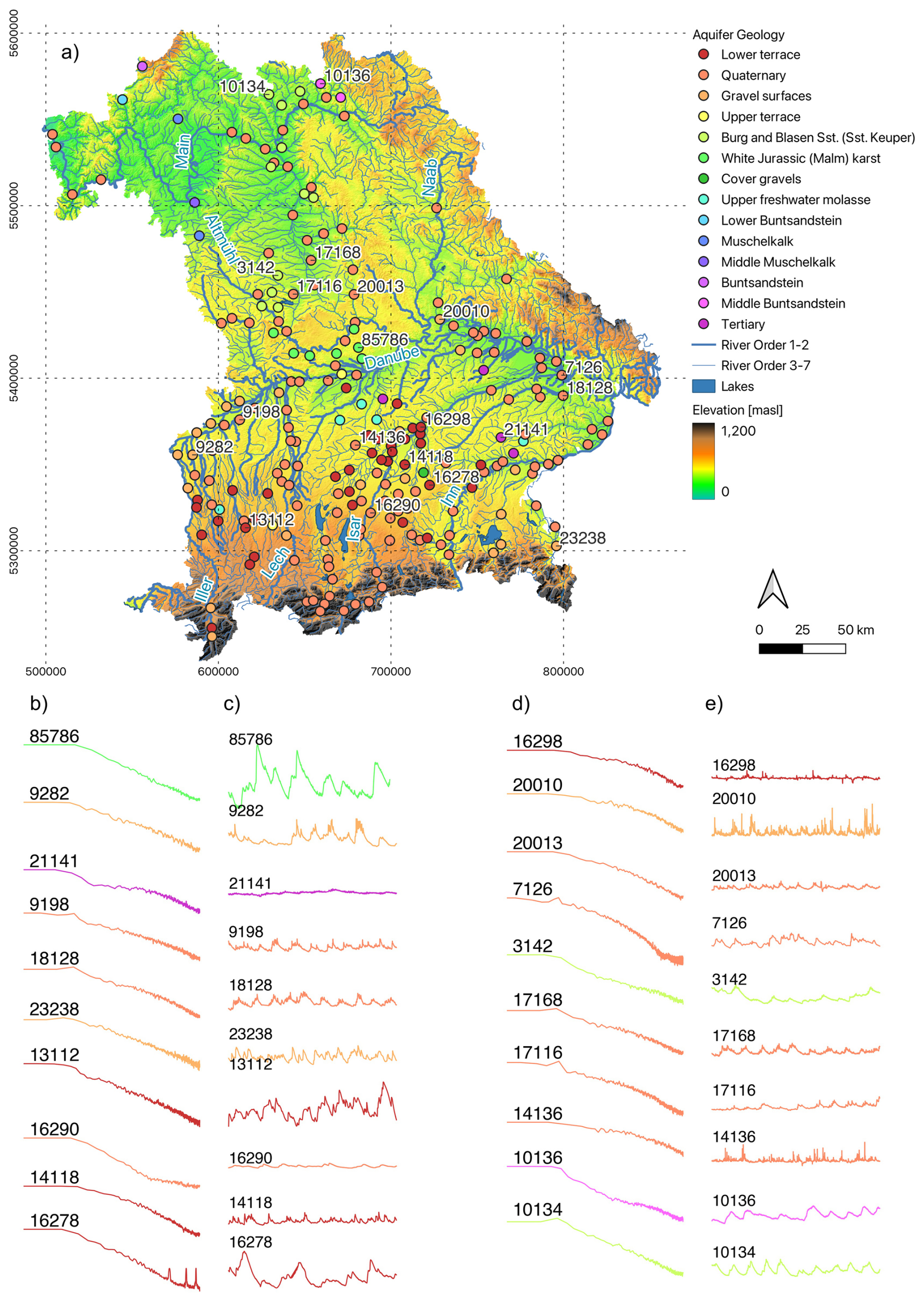
Figure 1 (a) The German state of Bavaria with the locations of the shallow groundwater observation wells from the state monitoring network including their aquifer geology. The digital elevation map was acquired from an SRTM data base (OpenTopography, 2013) while the rivers and lakes were provided by the German Federal Institute for Hydrology (BfG) and downloaded from their geopoartal (German Federal Institute for Hydrology – BfG, 2022). Coordinate reference system EPSG:25832 – ETRS89/UTM zone 32N. (b, d) Spectrum of groundwater level time series, (c, e) corresponding groundwater time series.

2.2.3 Transformation of time series into frequency domain (Fig. 2a and b)

Power spectra of head and recharge time series were estimated with Welch's method (Welch, 1967), with segment periodograms computed as the magnitude squared of the Fast Fourier Transform (FFT). Some exemplary time series of groundwater head spectra are depicted in Fig. 1b.

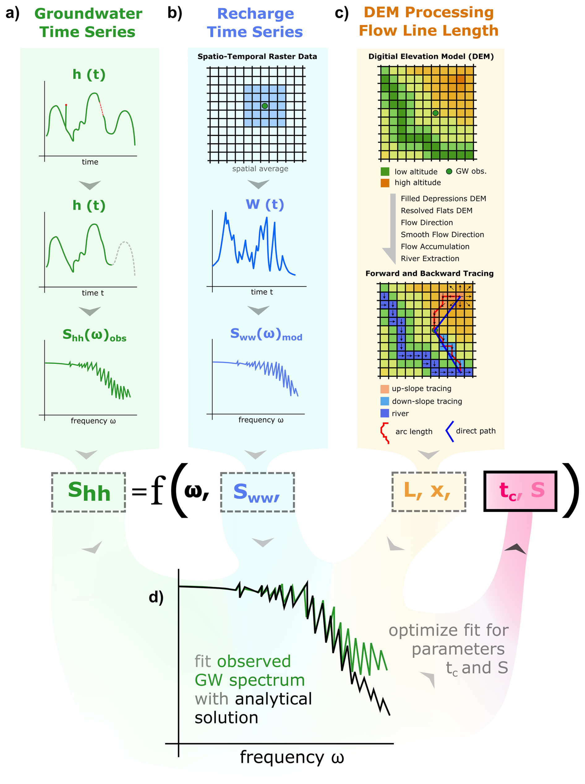
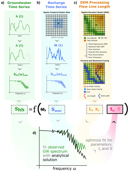
Figure 2 Overview of the spectral analysis (SpA) workflow. The aim is to acquire aquifer parameters based on the spectral response of groundwater and recharge time series, accompanied by geometric information of the aquifer (flow line length) derived from DEM processing. (a) Processing of groundwater level time series and transfer to frequency domain, (b) extraction of recharge time series from spatio-temporal simulations of the mesoscale hydrological model mHM and spatially averaged for shaded region, (c) DEM processing and consecutive flow line (FL) estimation, (d) measured groundwater level spectrum fitted with semi-analytical solution with t_c and S subject to optimization.

2.2.4 Estimation of Flow Line Length (Fig. 2c)

Using the semi-analytical solution for the spectrum from Liang and Zhang (2013) requires knowledge about the aquifer length L (from water divide to the river intersecting the well location) and the position x of the groundwater observation well along this transect.

The estimation of the flow line length (FLL) is solely based on DEM (digital elevation model) data. Required processing steps are similar to a watershed delineation with geospatial libraries. In a first step, data gaps in the DEM with a resolution of roughly 70×70 m (OpenTopography, 2013) were filled and a flow direction map was calculated providing the drainage direction for each cell. It serves as a basis for calculating the flow accumulation and by that the river network. Within that process, the flow accumulation threshold determines the complexity of the resulting river network. A large threshold (e.g., 1000) generates a coarser dendritic network and small creeks disappear (purple and blue in Fig. 3). While a smaller value of 100 results in a denser river network with several sub-catchments (orange Fig. 3) and head water catchments (Fig. 3c).

The selection of an appropriate threshold depends not only on the geological and geomorphological context, but also on the intended application of the resulting river network. A low threshold includes smaller channels and headwater streams in the network. These channels may be intermittent or ephemeral, especially in hilly terrain with deeper groundwater tables, whereas in flat areas with shallow groundwater tables even small channels may remain continuously connected to groundwater. As a result, these streams may not always maintain a connection to the groundwater table and may not consistently exhibit effluent conditions. We evaluated three thresholds (100, 500 and 1000) and compared the resulting networks with the official drainage network provided by the German Federal Institute for Hydrology (German Federal Institute for Hydrology – BfG, 2022). A threshold of 1000 turned out to be the best compromise: The resulting network exhibits the highest agreement with the official drainage network and provides a realistic representation of a river system composed of perennial streams that are regionally well connected to the aquifers. This connectivity is essential for satisfying the boundary conditions of the analytical solution (see Eq. 4), to which the spectra will later be fitted.

Next, we approximate the flow lines (FL) by tracing the path of the water particle along the surface (DEM) starting at the observation well down-slope following a flow direction map towards the river (blue, Fig. 2). For the upper part, the part between the well and the water divide, the flow direction was reversely applied, i.e., the directional vector of each cell was rotated by 180°, then followed from cell to cell and finally stopped when a summit was reached, leading to a unique uphill path (red, Fig. 2). Real groundwater paths can be very complex and are usually unknown without detailed on-site experiments on the catchment scale. Since our study has a regional focus, we decided to use flow direction maps derived from the DEM, automate the process and obtain estimates of the FL for a few hundred wells without manual inspection of each hydrogeological scenario. The used flow direction maps, though, are often very noisy, in particular in flat regions. In order to remove noisy patterns, avoid unreasonably short flow lines and obtain robust estimates, we smoothed the flow direction map (Appendix A1).

The actual path of the water particle along the hill slope (from water divide, intersecting the well towards the river) represents the longest possible path to be obtained with our method which we called the “arc length” (Fig. 2c), while the shortest and straight distance is called the “direct” path. We considered the “direct” path as more appropriate since the geomorphological surface introduced curves in the estimated flow paths which are presumably not present in the subsurface flow paths, thus we considered the “direct” path as better suited. A detailed example comparing different FLL can be found in the Appendix A2. The sum of the length of both parts is then equal to the flow line L_GW and the length of the upper part determines the location of the groundwater observation well x_GW (for water divide x=0 and river x=L_GW).

The SpA was performed on three different parameter combinations, leading to relatively short, medium and long flow lines. The resulting differences for t_c, x and L are presented in the Appendix as well as results for S and T (Appendix A3 and A4). Since the estimation of t_c once again proved to be robust-showing little sensitivity to the choice of flow lines (Appendix A3), as demonstrated previously by Houben et al. (2022) – we selected a parameterization representative of an intermediate FLL.

Figure 3 Maps of different geomorphological settings in the study region (a, b, c) showing the resulting river network for different flow accumulation thresholds. The DEM, which was the basis for the watershed analysis, is provided as background map with elevation in meter above sea level (masl). In addition, a river network acquired from the BfG (German Federal Institute for Hydrology – BfG, 2022) is provided to compare it to the extracted river from flow accumulation. (d, e, f) Zoom to three observation wells and their identified flow lines for threshold 1000 (downward toward the river and upward towards a summit). Depending on the chosen threshold, the flow line would stop earlier or later when it reached a stream.

2.2.5 Parameter Optimization and Evaluation (Fig. 2d)

Having groundwater level and recharge spectra in addition to estimates for L at hand, the semi-analytical solution was fitted to the observed head spectrum to finally obtain the response time t_c. The fitting of the analytical solution to the observed spectrum was accomplished through an iterative optimization process minimizing least-squares between observed and analytical spectrum to find optimal parameters, t_c and S. Due to the method, the contribution of lower frequencies to the spectra were weighted stronger during optimization than the corresponding ones of higher frequencies. Consequently, the fitted spectra matched better with the observed spectrum for low frequencies (left part in the log-log spectrum plots) while the deviation between both spectra generally appeared at high frequencies (right part of the spectrum plots).

2.3 Software and Tools

Python scripts to reproduce the full workflow are available via Zenodo (Houben, 2026). For the spectral analysis part a python library called AquiPy was developed, which is open source and available on GitHub (https://github.com/timohouben/AquiPy, last access: 4 September 2026; HESS-v0.1) and should be referenced via Zenodo (Houben, 2025).

The AquiPy library allows to handle and pre-process time series (interpolation, detrending), harmonize the recharge and groundwater level time series, calculate the spectra and fit the semi-analytical solution to the observed spectrum of the groundwater levels. Furthermore, the library was used to perform the flow line length estimation based on a digital elevation model (DEM).

3 Results

3.1 Groundwater Level Spectra

209 time series of groundwater levels were finally analyzed, their spectra were generated and fitted with the analytical solution following the workflow presented in the Fig. 2. Figure 4 depicts a random choice of 48 spectra calculated from observed groundwater level time series (black) and the corresponding fits of the analytical solution S_hh Fit (blue).

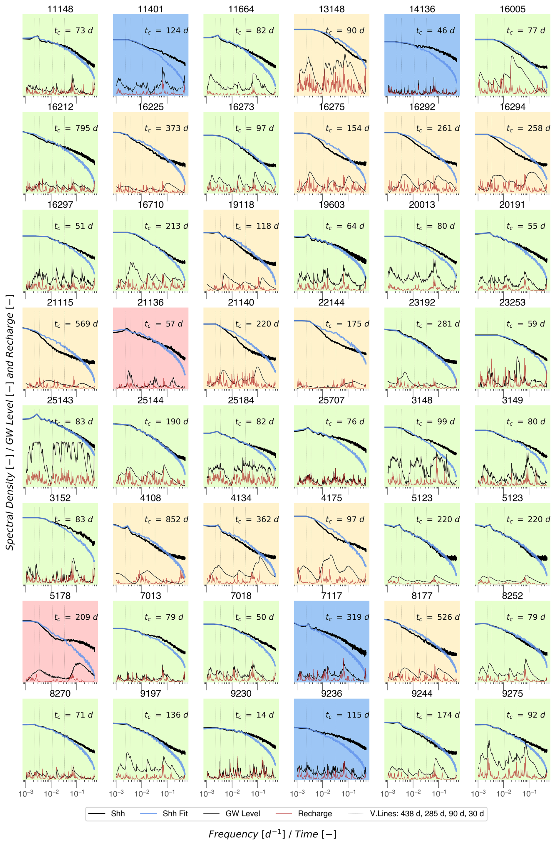
Figure 4 A random choice of 48 groundwater wells from the analysis. Each subplot showing the groundwater level (black line at the bottom), the corresponding spectrum S_hh (black spectrum), the extracted and averaged recharge (red line) from which the spectrum S_ww was used for the fit of the analytical solution S_hh Fit (blue spectrum).

The general shape of most of the spectra is similar, showing a plateau at low frequencies (left part of the spectrum) while gently decreasing for frequencies larger than a specific cut-off frequency. The low frequency regime describes the long time behavior of the groundwater time series. At intermediate frequencies, the onset of the filtering behavior and the response time can be identified. From the mid to the high frequency regime, filtering properties of an aquifer become visible. Many spectra show breakpoints which are far on the left-hand side of the spectra, some of them even hardly to identify. Weather this breakpoint becomes clearly visible depends on the filtering properties of the aquifer and the length of the investigated time series, as found by Houben et al. (2022). Even when a breakpoint is not clearly visible, the response time can be estimated since the recharge spectrum is considered in conjunction, assuming that the time series are long enough in relation to the aquifer response time t_c.

Partly there are differences between the spectra for frequencies larger than the cut-off frequency. Visual inspection of these spectra reveals four distinct GoF (Goodness of Fit) categories (Fig. 5). When the observed S_hh and theoretical spectra S_hh Fit exhibit close alignment across the entire frequency range, the result is classified as a “good fit”. If the observed spectrum S_hh exhibit steeper slope than anticipated in the theoretical spectrum S_hh Fit they are labeled as “overestimation”. These spectra show a stronger filter effect leading to generally smoother corresponding groundwater time series. In contrast, for observed spectra S_hh with a weaker slope, the fitted spectra S_hh Fit are “underestimating” the actual conditions, thus representing a groundwater system acting as a weaker filter than anticipated. Lastly, there are spectra that show a second plateau for medium frequencies or intermittent shape which is not reproducible by the theoretical spectrum, therefore labeled as “irregular”.

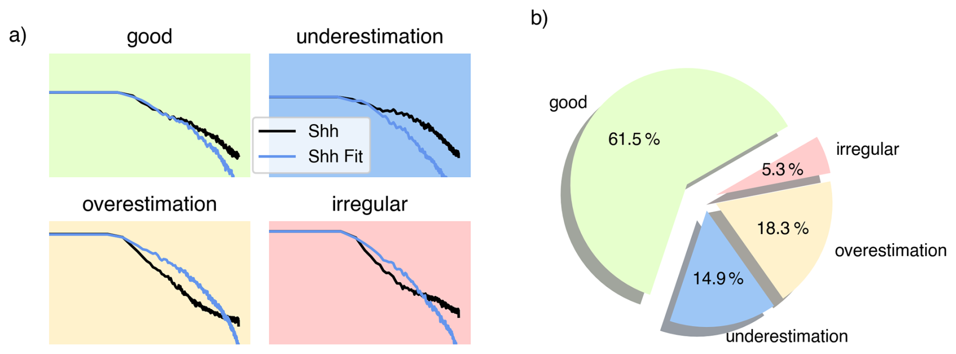
Figure 5 Evaluation of the goodness of the fit. (a) The four categories (good, underestimation, overestimation, irregular) and a representative example from the results. (b) Percentage of wells determined for each category.

Approximately 60 % of the spectra received the label “good fit”. In these cases, we can conclude that the theoretical model based on the Dupuit approximation captures the dynamic behavior of groundwater very well. Around 15 % of the observed groundwater spectra underestimate frequencies larger than $\mathrm{1}/\mathrm{30}$ d (right part of spectrum, see vertical line corresponding to 30 d in Fig. 4), showing a weaker filtering effect that anticipated from the theoretical spectra. Around 19 % of observed spectra show an overestimation in the mid-range frequency (corresponding to 1 year–1 month), indicating a stronger filtering effect than in theory. The remaining part, around 5 %, shows irregular spectra, where the theoretical spectra deviate across large parts of or even the whole frequency range.

Four examples of time series from groundwater wells, their recharge, the resulting spectra and the results of the SpA can be found in the Appendix A5, A6, A7 and A8.

3.2 Intermediate Frequency Regime: Identification of Aquifer Response Times

Considering the categories good and underestimation, half of the groundwater wells (52 %) show response times between 30 to 100 d, while 26 % have response times between 100–200 d. The majority (around 84 %) of the estimated response times from the analyzed aquifers of the considered categories range from approximately 30 d (1 month) to 300 d (about 10 months, Fig. 6a) which is consistent with the results presented in Kumar et al. (2016).

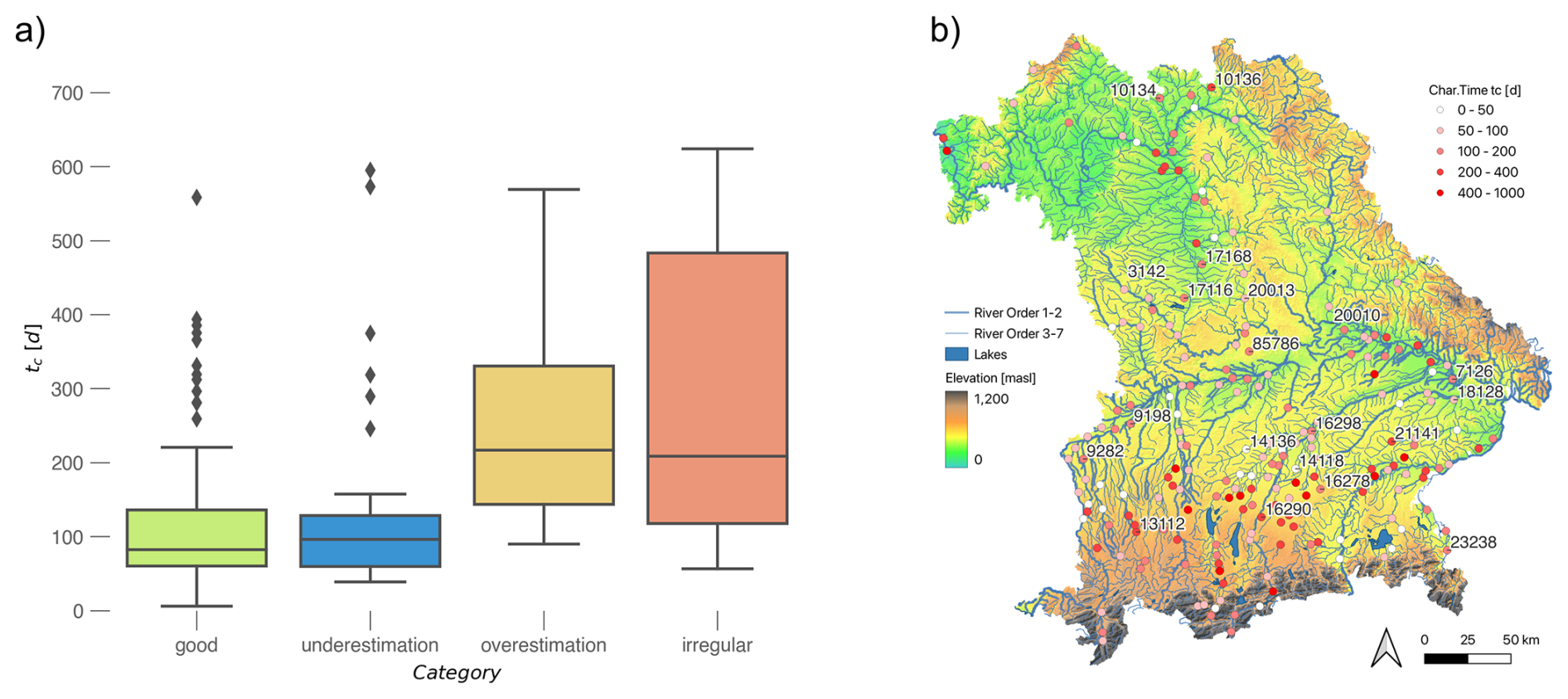
Figure 6 (a) Box plots of resulting aquifer response times for each category. Y-limits were trimmed and three outliers were cut off. (b) Map of Bavaria with SRTM (OpenTopography, 2013) as basemap and rivers from German Federal Institute for Hydrology – BfG (2022) showing the spatial distribution of obtained t_c.

Two clusters can be identified. A cluster with shorter response times of about 70 to 130 d (2–5 months) and a second cluster with response times ranging approximately from 130 to 340 d (5–10 months). The first cluster predominantly comprises data from shallow groundwater wells (category good fit, underestimation, Fig. 7) which show shorter response times, indicating a relatively rapid reaction to recharge events. These wells are predominantly located in unconsolidated Quaternary sedimentary formations such as Lower Terraces and gravel plains, which are characterized by high hydraulic conductivities, facilitating a direct transmission of recharge signals (Fig. 8).

In contrast, the second cluster originates from data from deeper groundwater wells (category overestimation, irregular, Fig. 7), which exhibit longer response times (Fig. 6), suggesting a more attenuated response to recharge. These wells are commonly located in consolidated formations such as Buntsandstein, Muschelkalk, and the Tertiary, where medium hydraulic conductivities and medium to high storativities likely contribute to a stronger damping of high-frequency recharge fluctuations (Fig. 8). Part of the attenuation in this cluster may also reflect the deep-vadose-zone effects discussed in Sect. 4.2. A correlation of aquifer geology to the GoF categories could not be identified (Appendix A9).

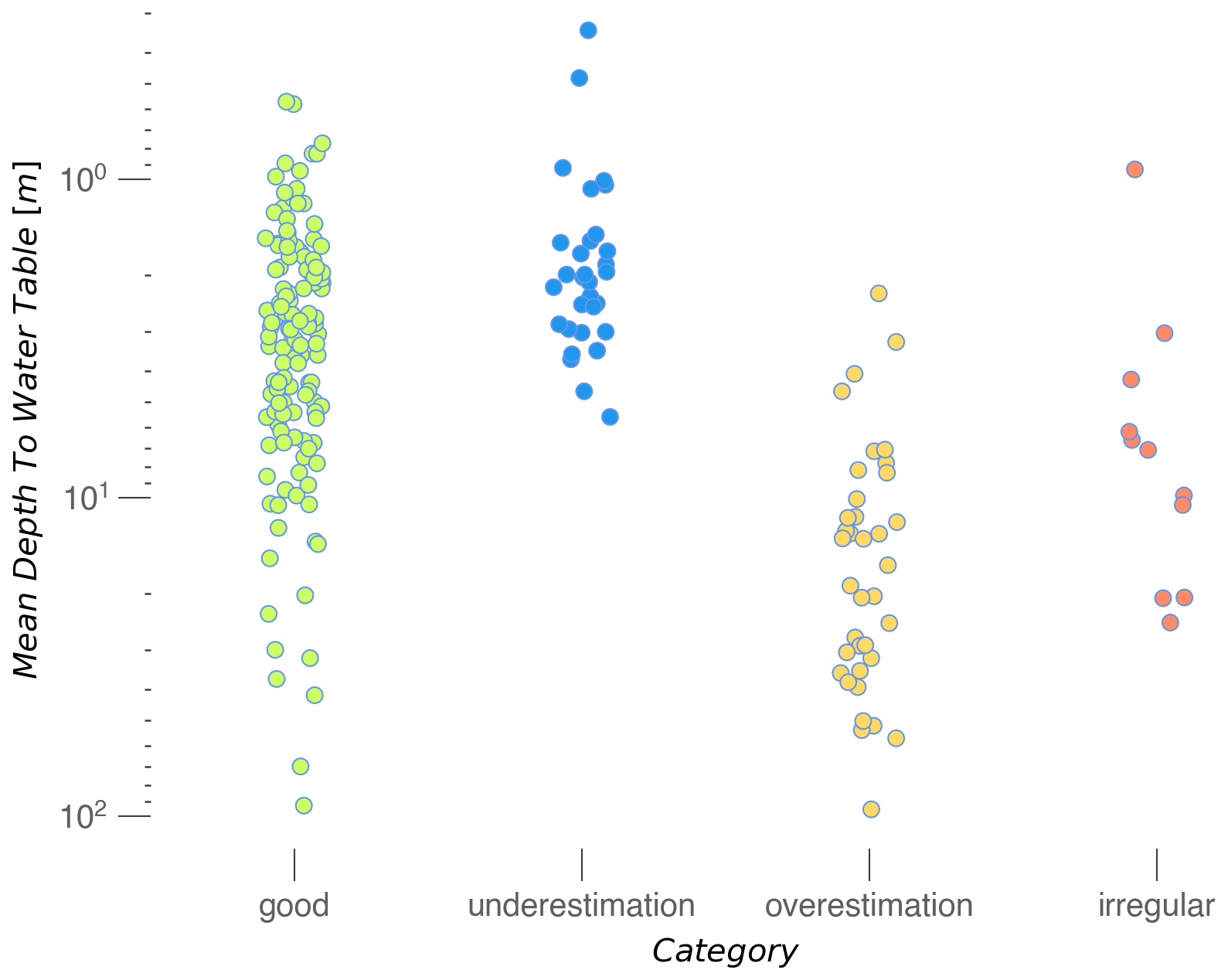
Figure 7 The four categories of the GoF in relation to the mean depth to the groundwater table. Good fitting spectra appear for across all depths. Shallow wells tend to be underestimated while deeper wells tend to be overestimated.

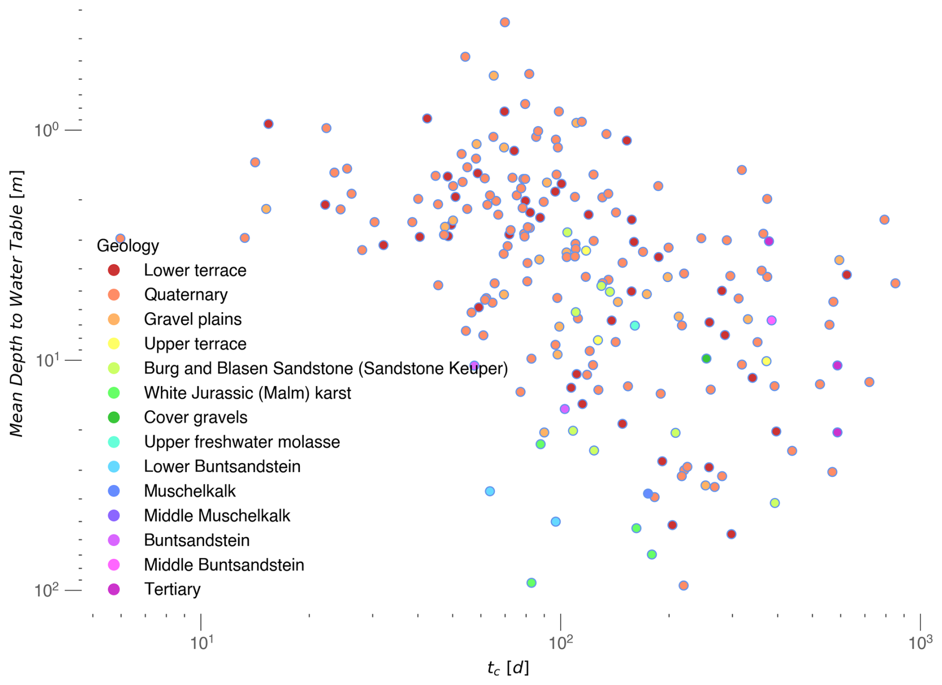
Figure 8 Scatter plot of depth to the water table (m) versus aquifer response time t_c (days), categorized by aquifer geology. Each point represents a groundwater well, with colors indicating different aquifer types.

3.3 High Frequency Regime: Filtering Behavior

Groundwater level fluctuations characterized by less high-frequency content (category overestimation, indicating a stronger filter) tend to occur at greater depths, whereas fluctuations containing more high-frequency components (category underestimation, weaker filter) are generally associated with shallower water tables. This behavior is illustrated by maps in Fig. 9. The left panel presents wells for which the theoretical spectra showed a good fit to the observed spectra. These wells are distributed throughout Bavaria and exhibit the full range of depths to the water table.

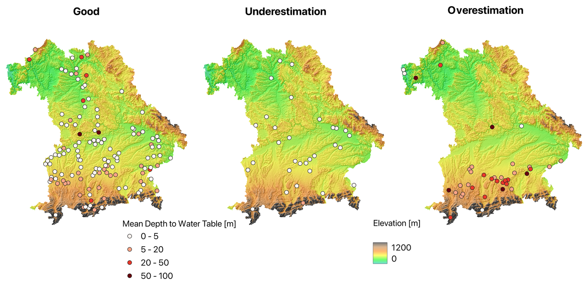
Figure 9 Spatial distribution of wells separated by GoF (Goodness of Fit) categories. The well locations are plotted together with the elevation map and markers for the GW wells, which are color-coded by depth to the water table.

The middle panel, representing the underestimation cases, consists predominantly of wells with shallow water tables. Underestimation occurs when the model does not fully capture the high-frequency variability, for example due to a dynamic groundwater recharge with more short-term fluctuations than assumed in the semi-analytical solution. Despite this limitation, the method still provides a good estimate for mid-range frequencies and with that groundwater response times on monthly to seasonal scales. Consequently, the inferred characteristic response time t_c remains a robust estimate.

The right panel highlights overestimation cases, which occur mainly in the southern and more elevated parts of the study area, where deeper groundwater tables are prevalent. Overestimation is observed in around 18 % of cases, where the semi-analytical solution predicts greater short-term variability than observed, indicating a stronger filtering effect than in reality. This could result from missing mid-term variability in the input signal (recharge) or unaccounted storage effects that further dampen mid-term fluctuations.

While the Transmissivity T and Storativity S are outcomes of the fitting workflow, they have not been discussed in detail in this study. The reason for this decision is that previous research (Houben et al., 2022) has demonstrated that especially T is highly sensitive to the length of flow line (FLL=L, see Eq. 6), leading to considerable uncertainties in their estimation (Appendix A4), as well as to the recharge time series taken for the parameter inversion. Therefore, we suggest further studies to improve the accuracy of the estimation of the FLL and the recharge time series. Additionally, considering lateral groundwater flow or aquifer leakage might enhance the predictive power of the semi-analytical solution, though this data are difficult to acquire and hard to integrate into analytical solutions. Exploratory modeling approaches incorporating leakage or lateral inflows could quantify these influences and their sensitivity within the spectral approach.

4 Discussion

This study introduces a novel spectral analysis method as part of a workflow to estimate characteristic response times of groundwater systems. These response times reflect how rapidly groundwater levels respond to changes in recharge or extraction and serve as a critical indicator of aquifer resilience under climatic and anthropogenic stresses. We applied this approach to approximately 200 groundwater level time series across southern Germany, integrating modeled recharge data and hydrogeomorphic parameters derived from digital elevation models. Our findings demonstrate that the semi-analytical spectral solution generally provides a strong fit to observed groundwater spectra and allows robust estimation of response times, which predominantly range from 30 to 300 d across shallow Bavarian aquifers (>100 m depth).

Within groundwater level spectra, three frequency regimes are distinguished: The low-frequency regime corresponds to long-term seasonal behavior, while intermediate frequencies reveal the onset of filtering related to the groundwater response time. In other words: As the aquifer acts as a low pass filter, low frequency components are mostly unaltered while the recharge signal passes the subsurface. The intermediate frequency band corresponds to the break point where the aquifer's low pass filtering begins to attenuate the input signal, which, in turn, corresponds to the system's characteristic time. The high-frequency regime exposes the aquifer's full filtering capability. While the model fits most spectra well, deviations primarily occur in the high-frequency regime (corresponding to less than 30 d period), which suggests the semi-analytical solution may not fully capture rapid recharge and river level fluctuations or effects of processes such as anthropogenic withdrawals and lateral groundwater flow.

At locations with stronger filtering than estimated (overestimation), actual groundwater recharge dynamics may be less variable than modeled by the mesoscale hydrological model mHM. Conversely, weaker filtering behavior (underestimation) likely indicates more dynamic recharge fluctuations than anticipated. These observations highlight potential limitations of the recharge inputs and imply that the method may also serve as a tool for evaluating distributed hydrological models.

4.1 Regional Flow Connectivity and Temporal Recharge Uncertainty

The assumption that recharge is spatially constant across a hillslope serves as a premise for deriving semi-analytical solutions under the Dupuit assumptions, as established by Liang and Zhang (2013). Their model treats groundwater flow along a 2D vertical transect with spatially consistent recharge but does not account for topographic or subsurface heterogeneity. However, this simplification may fail to represent real-world hydrogeological dynamics where spatial variability in connectivity significantly impacts the observed groundwater response.

Tóth (1963) introduced three distinct flow systems: local, intermediate, and regional in small basins. Local systems are bounded by topographic divides, intermediate systems bridge between local units and regional systems govern large-scale groundwater movement. Crucially, within these configurations, recharge and discharge zones alternate spatially, such that only a fraction of the hillslope contributes to baseflow for a connected stream. Consequently, water may be sourced from distant uphill recharge areas via regional flow pathways rather than being directly fed by local infiltration.

Following this, two primary sources of uncertainty can attributed to the modelled groundwater recharge:

• Spatial mismatch. The spatially averaged recharge used to construct the spectrum may not reflect actual recharge patterns, leading to inaccuracies in estimating characteristic response time t_c and spectral fitting quality.

• Temporal mismatch. Short-term fluctuations (<30 d) impose upward pressure on the spectrum's right-hand tail due to their influence on transient response. While these do not significantly alter mid-to-low frequency components (30–90 d range), a notable deviation at mid-frequencies suggests overestimation of low-frequency dynamics, potentially resulting in overestimated or prolonged t_c.

Only the category good fit captures the precise characteristic response of the aquifer, although we consider the category underestimation as still suitable for the estimation of longer time scales.

In practice, the current study mitigates spatial uncertainty by focusing exclusively on shallow wells (<100 m depth) where local recharge dominates and regional flow is less likely. Nevertheless, even here, confined aquifers may hinder vertical flow, allowing distal sources to bypass local recharge entirely. Hence, this method remains most applicable for unconfined sediments rather than fully confined aquifers. A related caveat regarding the possible influence of the deeper subsurface on the estimated response times is discussed in the following section.

The categorization into four goodness-of-fit groups (good fit, underestimation, overestimation, irregular) enables a systematic evaluation of spectral match quality and the associated parameter uncertainty. This framework allows us not only to quantify the fidelity between observed and fitted spectra but also to identify when limitations arise – particularly in mid-frequency range discrepancies indicating potential misrepresentation due to spatial connectivity or temporal scale mismatch.

4.2 Related Approaches

Bloomfield and Marchant (2013), Kumar et al. (2016) and Ebeling et al. (2025) examined the cross-correlation between the Standardized Precipitation Index (SPI) and the Standardized Groundwater Index (SGI), using the relationship to estimate how groundwater levels respond to meteorological drivers. Their analysis effectively incorporates the delay introduced by the unsaturated vadose zone, allowing for a response time evaluation that accounts for this lag. By contrast, our method uses recharge simulated by mHM (which accounts for soil moisture dynamics and percolation in the shallow, rooting-zone soil column) directly as the input, which reduces the influence of near-surface vadose zone dynamics on the estimated response time. Because mHM's soil-moisture and baseflow parameterizations are calibrated against near-surface soil moisture and catchment discharge rather than groundwater head (Boeing et al., 2022), this reduction is likely incomplete for wells with a deep water table, where transit through a thick, well-specific unsaturated zone may impose additional low-pass filtering not represented in the mHM recharge signal (Tsypin et al., 2025). We therefore treat t_c estimated for such wells as an upper-bound, composite estimate rather than a purely aquifer-intrinsic value.

Comparing these two approaches, it becomes obvious why response times from Kumar et al. (2016) and Ebeling et al. (2025) exhibit longer times than the response times obtained by the spectral analysis approach. Furthermore, the correlation of longer times in relation to the depth of the well is more pronounced since the vadose zone plays a significant role. Beside this, our spectral analysis approach uses a full spectrum wide comparison over multiple frequencies and finds a best fitting spectrum, in contrast to Kumar et al. (2016) and Ebeling et al. (2025) where a best fitting accumulation period was calculated. Furthermore, our approach links the response time directly to physical properties of the aquifer since corresponding (and simplified) equations of groundwater flow are used.

Current practices in groundwater drought analysis (e.g., Kumar et al., 2016; Ebeling et al., 2025) typically rely on accumulation times derived from the correlation between standardized indices (SPI/SPEI vs. SGI) and these metrics primarily provide insight into the “hydrological lag” which is the time required for a climatic deficit to propagate through the soil and vadose zone to reach the water table. In contrast, the characteristic response time t_c derived by the presented spectral analysis workflow is intended to characterize primarily how the saturated aquifer processes and moderates that stress once it has arrived.

While the vadose zone is potentially the dominant driver of hydrological signal filtering (e.g., Liesch and Wunsch, 2019; Tsypin et al., 2025) the saturated aquifer independently functions as a low-pass filter governed by its intrinsic hydraulic properties: transmissivity T and storativity S. Although confined aquifers possess limited pore-space elasticity, resulting in low storativity, a concurrently low T can still yield significant characteristic response times. Physically, this buffering occurs through the elastic expansion of the aquifer skeleton and the vertical oscillation of the water table. Whereas the unsaturated zone primarily introduces a transport delay, the saturated zone attenuates the signal through hydraulic diffusion. As noted above, using mHM-derived recharge as input reduces, but does not fully remove, the influence of the unsaturated zone on the estimated response time. It should also be noted that not all observation wells yielded a high-quality fit, suggesting that localized recharge estimations may be subject to greater uncertainty at specific sites.

Mathematically and physically, these two metrics describe different segments of the hydrological cycle. The accumulation time is a statistical window representing the system's total memory (soil + vadose zone + aquifer), whereas t_c is an intrinsic hydraulic parameter defined by the aquifer's dimensions and its ratio of storage to transmissivity. Consequently, high accumulation times do not necessarily imply long characteristic response times. A system may exhibit a multi-year accumulation lag due to a thick, slow-draining vadose zone, yet possess a short (e.g., <50 d), indicating that the saturated zone has little capacity to buffer against high-frequency fluctuations or localized abstraction stress.

We further note that t_c should not be equated with a lag time in the sense of time-to-first-response, nor does it quantify any asymmetry between the onset and decline of the groundwater response to a forcing event. Because t_c is fitted to the power spectrum of the head and recharge signals, it discards phase information and therefore describes only the frequency-domain strength of low-pass filtering, not the time-domain shape of the response. The pronounced asymmetry between rise and recession of groundwater heads – illustrated for streamflow by Kirchner et al. (2023) and for groundwater head specifically by Lee and Ajami (2023) – is accordingly not captured by t_c as defined here; characterizing it would require a complementary, phase-resolving or time-domain analysis, which we consider a valuable direction for future work.

4.3 Implications for Drought Evaluation

In the context of drought evaluation and management, the following holds:

• By using recharge time series (e.g., from mHM) rather than precipitation as the spectral input, our approach reduces the influence of near-surface soil-moisture dynamics on the estimated response time, helping managers distinguish surface-level delays from the intrinsic buffering capacity of the aquifer, bearing in mind that for deep wells the estimate may still include an unresolved deep vadose zone contribution.

• While accumulation times tell us when a drought begins to manifest in the groundwater, t_c reflects the aquifer's overall capacity to dampen fluctuations in recharge, whether deficits or surpluses. A short t_c suggests a flashy system that may reach critical levels quickly during a recharge failure but can recover rapidly after a single wet season. Systems with high t_c are better suited for sustaining abstraction during isolated dry years, but they require more strict long-term management to prevent entire depletion. Conversely, flashy systems with short t_c are highly vulnerable to immediate rainfall deficits but possess the advantage of rapid replenishment.

• For sustainable groundwater management, both values must be analyzed in conjunction. An aquifer with both long accumulation times and a high t_c represents a highly resilient strategic reserve. Conversely, an aquifer with a long accumulation lag but a short t_c is deceptively vulnerable: it may appear stable during the early stages of a drought, but once the deficit reaches the water table, the system lacks the hydraulic capacity to dampen the impact, leading to rapid level declines.

Beside the interplay of both measured, comparing groundwater response times with drought durations is another essential step. Short response times may lead to rapid water table declines during dry seasons, while long response times correspond to prolonged aquifer recovery, maintaining low-water conditions. Given climate change-induced increases in drought frequency and severity, flexible and regionally targeted groundwater management strategies are critical.

While response time provides valuable insight into aquifer resilience, additional indicators are necessary for a comprehensive assessment. We propose incorporating metrics such as the duration of water storage in the subsurface and the aquifer yield beside information on water abstraction rates. Future work will focus on identifying storativity S alongside t_c in order to evaluate the aquifer resilience comprehensively and quantifying associated uncertainties.

Overall, this spectral approach proves to be a powerful tool for characterizing groundwater system dynamics and offers important implications for assessing aquifer resilience under changing climatic conditions.

5 Conclusions

This study successfully demonstrates that spectral analysis of groundwater levels with semi-analytical solutions can robustly estimate characteristic response times across a large number of aquifers. Groundwater response times predominantly range between 50 and 300 d in the studied Bavarian systems. The semi-analytical solution for the spectral domain applies well to the majority of investigated groundwater time series. Furthermore, the correlation between groundwater depth and spectral filtering underlines the importance of aquifer characteristics in quantifying resilience to drought and recharge variability.

Incorporation of additional anthropogenic and hydrological factors, such as withdrawal rates, as well as improvements of FLL estimations and the recharge time series, is needed to further refine the estimation of aquifer parameters, including transmissivities and storativities.

Future research will extend these methods to include storage estimation, improving our understanding of aquifer vulnerability and informing water resource management in a changing climate.

Appendix A: Additional Figures

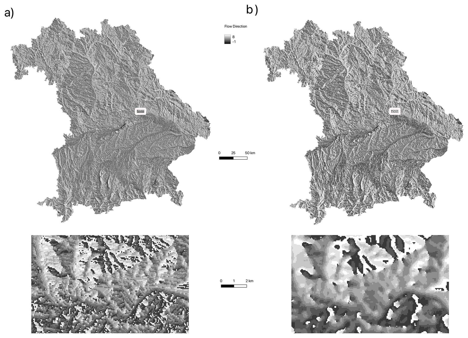
Figure A1 (a) Standard flow direction map derived from a DEM, (b) smoothed flow direction map. The flow direction was smoothed with a python function by averaging neighboring direction vectors over a specified “level” of neighborhood. Here, level 2 was used, meaning that two levels of surrounding cells where included, mapping back the average value to the center cell. The corresponding code can be found in the AquiPy package on GitHub https://github.com/timohouben/AquiPy (last access: 4 September 2026; HESS-v0.1).

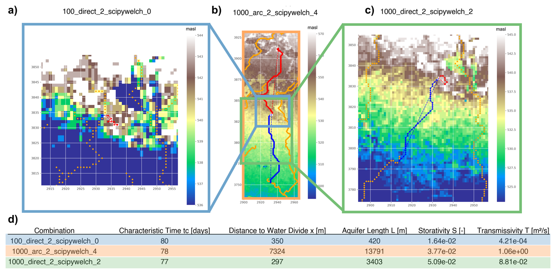
Figure A2 Resulting flow lines for three different parameter sets. (a) Flow lines generated with the smallest flow accumulation threshold (100), resulting in the shortest flow paths. Streams extend far into the hills, reducing the distance from the well to the nearest river (blue lines). With no smoothing applied to the flow direction, the upstream path terminates early (red lines). (b) The longest flow lines, produced using a higher flow accumulation threshold (1000). Here, rivers appear less dendritic, and the distance from the well to the river increases. Strong smoothing of the flow direction (level 4) causes the upstream segment to reach higher elevations. The arc length (indicated by stars) is used to measure the path, in contrast to the direct connection (dashed lines). (c) A parameter set that yields flow lines of intermediate length, which is selected for further analysis in this study. (d) A table summarizing the key values for each parameter set. The distance to the water divide x represents the distance from the well to the water divide. The aquifer length L is defined as the sum of the upstream and downstream segments.

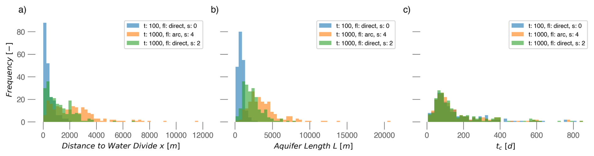
Figure A3 Flow line estimation results and spectral analysis results (histograms) for three different parameter configurations. The x axis label “Frequency” refers to the count of values for each bin. (a) Distance to water divide x and (b) aquifer length L as a result of the Flow Line Length estimation with different flow accumulation thresholds t, selection of flow lines fl and smoothed flow direction map s. Short flow lines are created when the flow accumulation threshold is small, because a dendritic river network is created. Direct flow lines connect the starting and end point of the flow lines with a straight line, while the arc length follows the whole flow path along the hillslope (i.e. the DEM). The higher the number for the smoothing of the flow lines, the longer the flow paths. (c) Resulting characteristic time t_c for the three parameter sets.

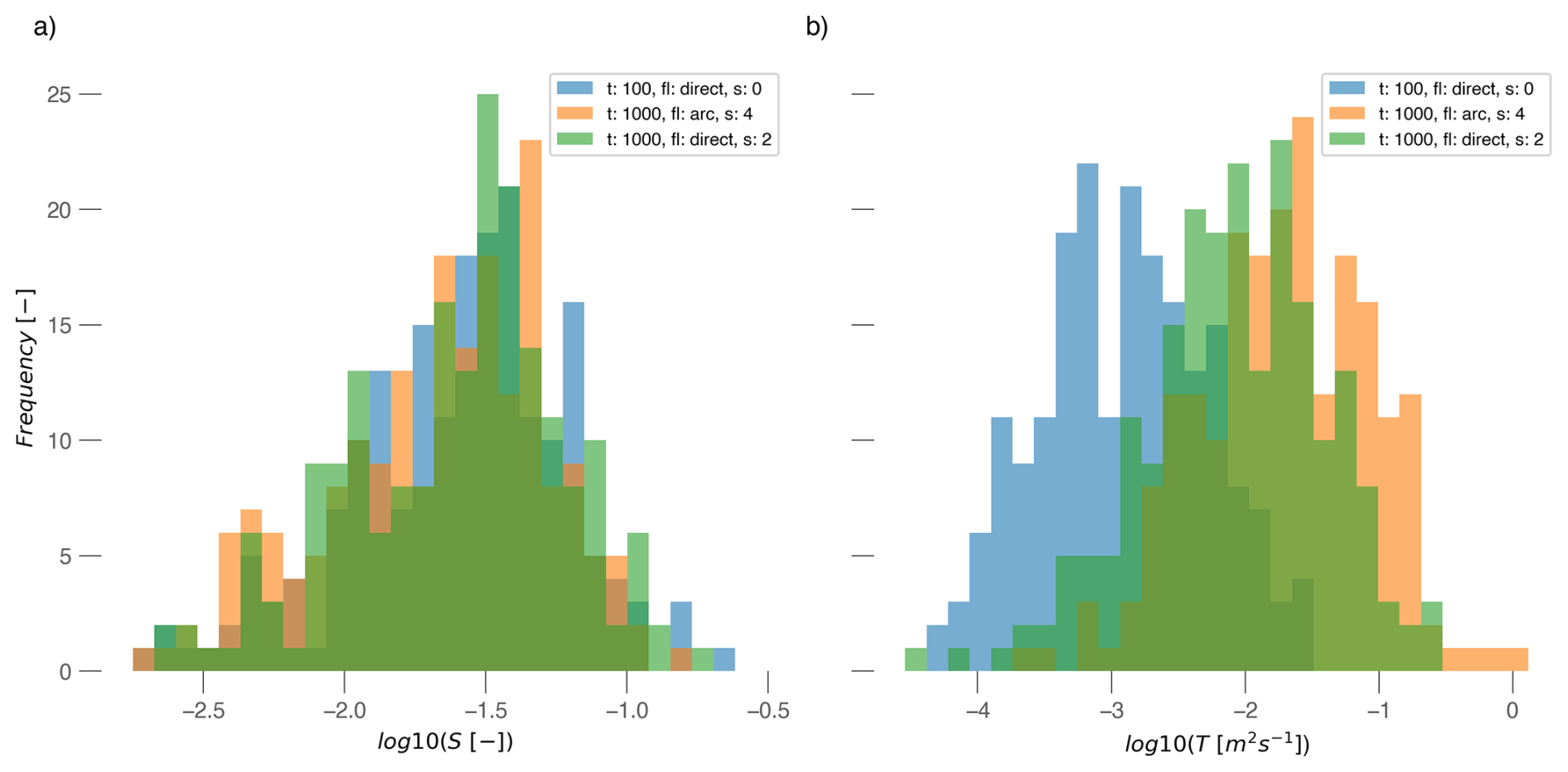
Figure A4 spectral analysis results for the three parameter sets for the flow line estimation. (a) storativity S and (b) transmissivity T. While resulting storativities differ only slightly, the transmissivities show stronger deviations due to different flow line lengths (= aquifer length) L.

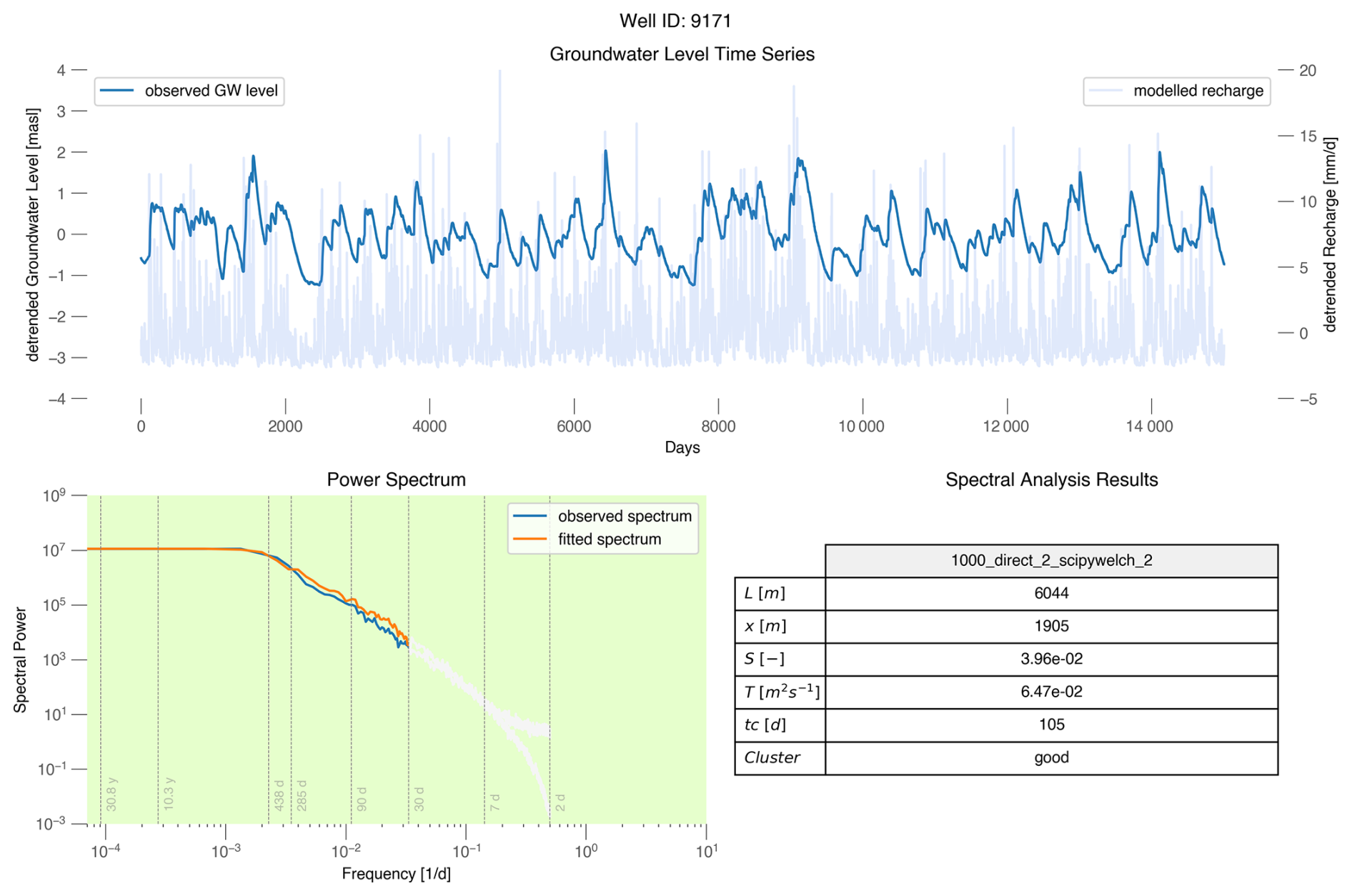
Figure A5 An example of a summary of analysis for a groundwater well of the category good fit. The figure shows the observed groundwater level time series and the modeled mHM recharge (Marx et al., 2021), the resulting power spectra for the observed groundwater level and the fitted spectrum with the semi-analytical solution. Only the colored part of the spectrum up to a frequency corresponding to 30 d was taken for the goodness of fit evaluation. The table summarizes the results of the workflow for the selected parameter set.

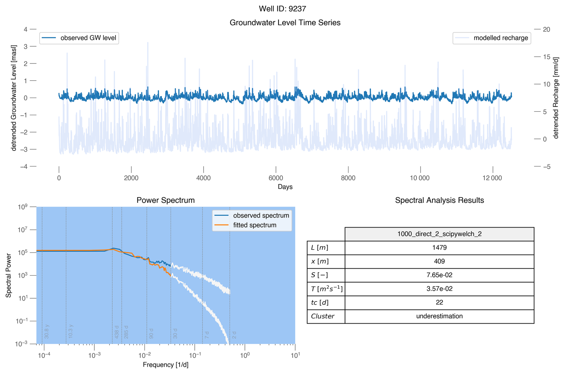
Figure A6 An example of a summary of analysis for a groundwater well of the category underestimation. The figure shows the observed groundwater level time series and the modeled mHM recharge (Marx et al., 2021), the resulting power spectra for the observed groundwater level and the fitted spectrum with the semi-analytical solution. Only the colored part of the spectrum up to a frequency corresponding to 30 d was taken for the goodness of fit evaluation. The table summarizes the results of the workflow for the selected parameter set.

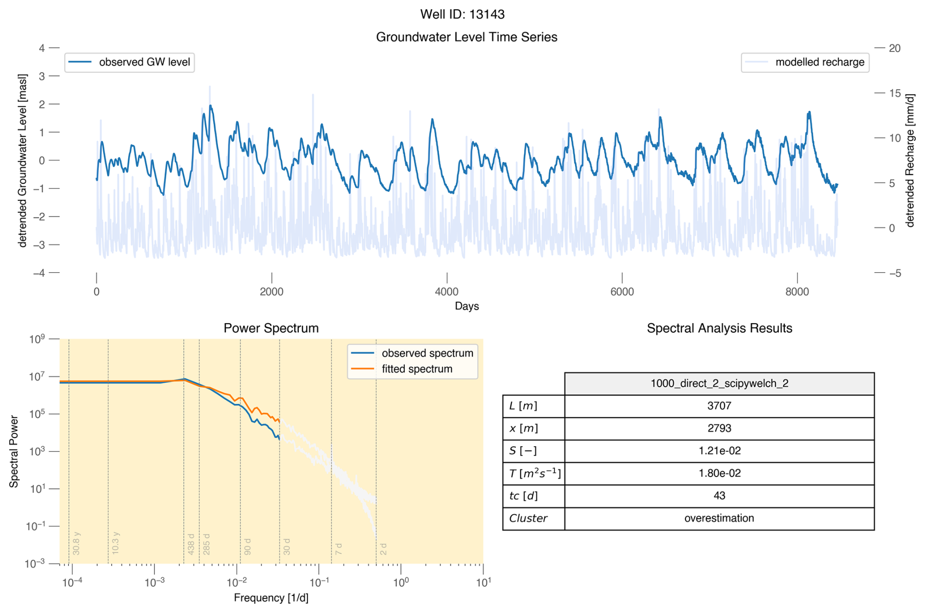
Figure A7 An example of a summary of analysis for a groundwater well of the category overestimation. The figure shows the observed groundwater level time series and the modeled recharge mHM (Marx et al., 2021), the resulting power spectra for the observed groundwater level and the fitted spectrum with the semi-analytical solution. Only the colored part of the spectrum up to a frequency corresponding to 30 d was taken for the goodness of fit evaluation. The table summarizes the results of the workflow for the selected parameter set.

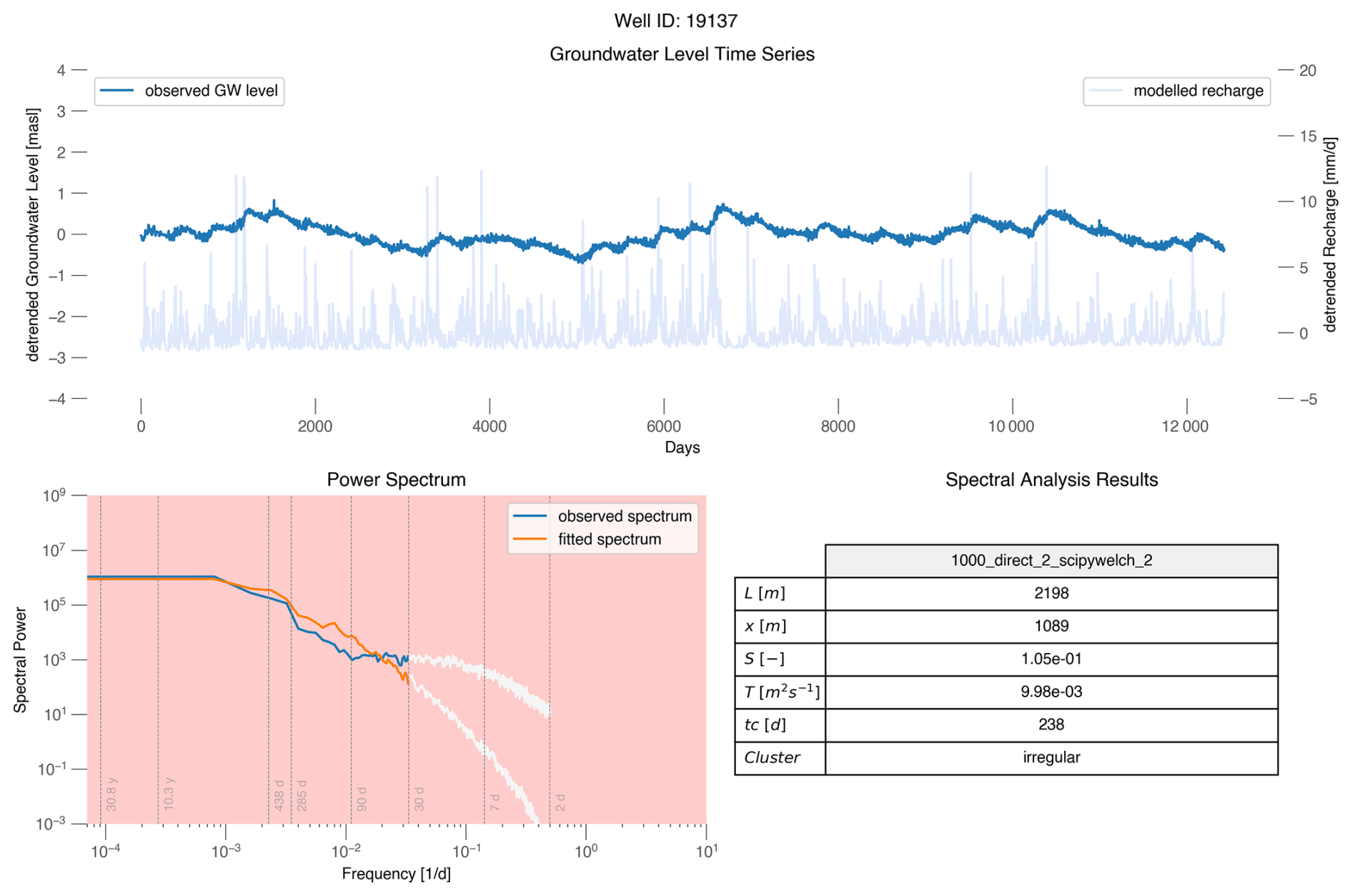
Figure A8 An example of a summary of analysis for a groundwater well of the category irregular. The figure shows the observed groundwater level time series and the modeled mHM recharge (Marx et al., 2021), the resulting power spectra for the observed groundwater level and the fitted spectrum with the semi-analytical solution. Only the colored part of the spectrum up to a frequency corresponding to 30 d was taken for the goodness of fit evaluation. The table summarizes the results of the workflow for the selected parameter set. In the presented time series and spectrum, multiple dominant frequencies can be observed: Long-term and multi-annual fluctuations with periods of decades, seasonal fluctuations with a period of a year and short-term fluctuations with periods of weeks to even days. The latter can be most likely attributed to barometric pressure changes in the atmosphere, as variations in summer are less than in winter times. The diverse set of present frequencies in the signal result in a complex shape of the spectrum with several breakpoints. Our simplified semi-analytical approach with a recharge product taken from a land surface model fails to capture the complexity of the processes of this groundwater level fluctuation and was consequently categorized as irregular.

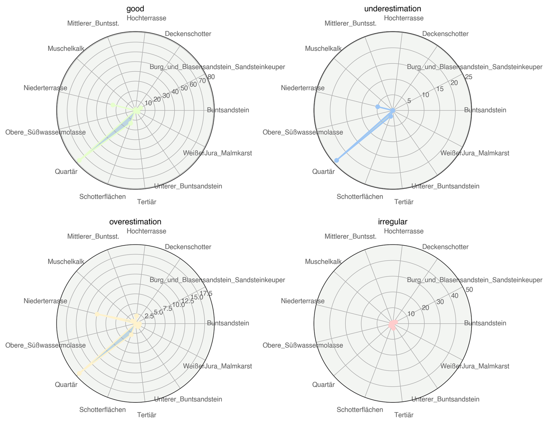
Figure A9 Spider plots showing the aquifer geology for the four GoF (goodness of fit) categories.