Technical note: HydroModPy (v1.0) – a Python toolbox for deploying catchment-scale shallow groundwater models

Despite the widespread use of physically based groundwater models, their deployment at the catchment scale remains challenging and time-consuming. HydroModPy was developed to address this gap by enabling automated and streamlined multi-site development of hydrogeological models at the catchment scale. This open-source Python toolbox facilitates the construction, execution, calibration, and analysis of unconfined shallow groundwater models. The current version integrates well-established geospatial tools, such as Whitebox Tools, and hydrogeological libraries with FloPy-driven MODFLOW-NWT simulations, along with optional particle-tracking and solute transport modules (MODPATH and MT3DMS), to provide a fully scriptable, end-to-end workflow. Automation is achieved through dedicated functions and classes capable of performing watershed delineation from digital elevation models, preparing spatial and temporal recharge forcings, generating computational meshes and vertical discretization schemes, assigning model parameters, and running simulations in steady-state or transient modes. The overall framework supports systematic and reproducible calibration routines that leverage subsurface data such as groundwater head measurements, as well as surface observations – including stream network maps and stream intermittency patterns – to constrain model estimates of aquifer hydraulic properties. Model outputs and provenance metadata are exported in standard geospatial formats to ensure interoperability and alignment with FAIR data principles. Built-in visualization tools and integration with Jupyter Notebooks support interactive exploration, teaching applications, and fully reproducible analyses. In this technical note, we present the HydroModPy architecture and its core functionalities, demonstrate model deployment across various hydrogeological contexts, and discuss ongoing and planned developments for future versions of this collaborative tool. The codebase is modular and extensible, making it suitable for adoption by a broad user community. Planned enhancements include tighter coupling with land-surface or ecohydrological models adding new numerical solvers, integrating advanced calibration and uncertainty quantification algorithms, and improving user interfaces to facilitate application in various environmental settings. HydroModPy contributes to improving the understanding of hydrogeological processes that are often poorly characterized or inadequately represented. It also provides valuable support for multidisciplinary education, particularly for those studying groundwater systems and their interactions with the surface in headwater catchments. Furthermore, this numerical framework can serve as a practical decision-support tool for public policy and water resource management, helping stakeholders address current and future groundwater-related challenges.

1 Introduction

Groundwater plays a fundamental role in sustaining ecosystems, supporting agriculture, and providing drinking-water supplies, particularly through its function as natural storage (Bierkens, 2015; McMillan et al., 2016). The management of groundwater resources and their interactions with the land surface require a robust understanding of subsurface hydrological processes, which is especially critical in the context of climate change, land-use changes, and increasing anthropogenic pressures (Blöschl et al., 2019). While global models can address the issue of water resources at large scales (Condon et al., 2021; de Graaf et al., 2017; Gleeson et al., 2020; Fan et al., 2013), considering hillslope processes in a modeling framework remains necessary for effective local management (van Jaarsveld et al., 2025; Wood et al., 2011; Fan et al., 2019). Catchment-scale hydrogeological models are a good compromise to represent both local processes and regional groundwater dynamics, helping researchers and decision-makers evaluate water availability, predict future conditions, and design sustainable management strategies (Clark et al., 2015). Consequently, the community requires flexible and scalable tools capable of supporting the development and deployment of groundwater models across diverse spatial scales, from headwater catchments to entire regions.

Catchment-scale groundwater modeling remains a complex and time-consuming task, often requiring specialized software, technical expertise, and the integration of diverse datasets. This complexity increases further when attempting to apply or deploy a modeling approach across multiple sites. The deployment of a hydrogeological model to new catchments is often limited by manual data handling, local parameter choices or site documentation (Wood et al., 2011; Clark et al., 2015). Systematic and reproducible workflows are needed to address these challenges and improve the deployment of groundwater models. While graphical user interfaces (GUIs) offer intuitive model development environments (Trefry and Muffels, 2007; Winston, 2009; Foglia et al., 2018), their transferability remains limited, and they often only provide restricted capabilities for systematically exploring model parameter sensitivity and uncertainty. Transitioning from GUI-based workflows to systematic script-driven approaches – characterized by automated, well-documented procedures for model setup, execution, and analysis – enables standardized management of data and parameters, fostering reproducibility and scalability (Pérez et al., 2011; Bakker and Kelson, 2009; Stacke and Hagemann, 2021; Velásquez et al., 2023).

In this context, a variety of tools have emerged within the hydrological and hydrogeological modeling community. These tools can be broadly classified into four main categories based on their objectives: (1) simplifying model execution, (2) enabling the coupling between different components or models, (3) automating model deployment, and (4) promoting FAIR (Findable, Accessible, Interoperable, and Reusable) principles (Wilkinson et al., 2016). First, tools that facilitate the input data processing (Gardner et al., 2018) and model construction and execution in hydrogeological modeling, such as FloPy (Bakker et al., 2016), streamline the process of setting up and running simulations. Second, coupling tools facilitate the integration of surface and subsurface hydrological processes or the orchestration of multiple model components. For example, GSFLOW (Larsen et al., 2022; Regan et al., 2015; Markstrom et al., 2008) explicitly couples PRMS (a precipitation-runoff model for the surface component) with MODFLOW (a groundwater flow model) to simulate their interactions; GSFLOW-GRASS integrates GSFLOW into the GRASS GIS environment to automate spatial preprocessing and the transfer of data between GIS and models; CWatM (Guillaumot et al., 2022) enables connecting a distributed precipitation-runoff model to MODFLOW or other simpler hydrogeological modules to explore the impact of spatially distributed recharge on subsurface behavior; and MARRMoT (Knoben et al., 2019) provides a multi-model orchestration platform to run, compare, and interface different hydrological and hydrogeological simulators within a single reproducible framework. Third, automated deployment solutions, such as those described by Lewis et al. (2018) and the Raven hydrological modeling framework (Craig et al., 2020), focus on replicability and scalability, allowing models to be efficiently applied across multiple catchments or regions. Finally, recent advances emphasize the adoption of FAIR principles to enhance transparency, reproducibility, and community engagement. Initiatives such as Community Workflows (Knoben et al., 2022), the eWaterCycle platform (Hut et al., 2022), and GroMoPo (Zipper et al., 2023) provide collaborative environments and standardized practices for sharing models and data.

Although numerous tools have been developed to address specific aspects of hydrogeological modeling, often with varying levels of complexity and scope, their integration into a coherent workflow frequently requires substantial user intervention. In practice, users often need to develop custom scripts and interfaces to connect model domain extraction, model setup, code coupling, model execution, deployment across multiple sites, and FAIR-compliant data management. While this flexibility allows adaptation to diverse applications, it can also increase workflow complexity and hinder reproducibility, portability, and large-scale deployment. This highlights the need for an integrated and adaptable toolbox that can bring these concepts together within a coherent workflow. Rather than a generic solution, such a framework should combine a high degree of automation and reproducibility with the possibility for user adaptation to site-specific data, assumptions, and objectives. In practice, this type of tool can support interdisciplinary Critical Zone studies by providing reproducible scripts, explicit model settings and metadata, and standardized outputs that can be readily exchanged with other disciplinary tools and workflows. This does not remove all disciplinary barriers by itself, but it provides a common technical basis that can facilitate collaboration between hydrogeologists and other Critical Zone communities (Gaillardet et al., 2018; Wang et al., 2025; Staudinger et al., 2019).

Here, we introduce HydroModPy, a Python-based toolbox designed to build, run, and calibrate hydrogeological models while importing and exporting both observed and simulated data. Its architecture and settings particularly support quantifying groundwater–surface connectivity. Thanks to the spatio-temporal simulation of groundwater flow and hydraulic heads, groundwater discharge zones naturally emerge, allowing for studying the dynamics of baseflow. This methodological approach enables the simulation of streamflow intermittency across the catchment, driven by the expansion and contraction of the stream network. In addition, the computation of transit times and the simulation of solute transport processes can be readily implemented within the proposed modeling framework. At this stage, HydroModPy is primarily tailored to unconfined shallow aquifers where hydrogeological boundaries roughly correspond to topographic divides, although flexibility is given regarding the delimitation of model boundaries. The toolbox facilitates parameter exploration, sensitivity analysis, and model calibration using optimization functions. Its modular structure and standardized workflow ensure seamless analysis and consistent interpretation of hydrogeological model outputs across different sites and simulation scenarios. This feature provides a significant advantage for comparing HydroModPy results with outputs from other hydrological models and observational datasets, such as those available from long-term observatories (e.g., Ackerer et al., 2023). HydroModPy achieves these functionalities by integrating open-source libraries for geospatial processing, groundwater flow modeling, and result visualization. The structure of this paper is organized into three main sections: (1) an overview of the general workflow, highlighting its key components and functionalities; (2) some examples demonstrating the capabilities of deployment in different hydrogeological contexts, including a survey of current applications worldwide, and a regional-scale deployment across multiple catchments; and (3) a discussion of limitations, future perspectives, and potential improvements, summarizing the contributions and relevance of the proposed tool for both academic and operational communities.

2 Workflow and code description

HydroModPy is structured into six main components: (1) watershed extraction defining the model domain area, (2) model conceptualization and preparation of input data for calibration, (3) parameterization of the hydrogeological model, (4) computation of groundwater flows, particle tracking and/or solute transport, (5) exporting of standardized outputs and visualization results and (6) compare outputs and data for calibration purposes (Fig. 1). The first five components are described in detail in the following five subsections (Sect. 2.1 to 2.5) and the calibration component in Sect. 3.2. It relies as much as possible on existing, well-validated, and widely used Python packages such as NumPy (Harris et al., 2020), pandas (McKinney, 2010) and xarray (Hoyer and Hamman, 2017), enabling users to interact with the model through a clear and consistent interface.

Figure 1 Workflow of HydroModPy, illustrating the organization and interconnection of Python scripts within the toolbox across six main stages: (1) watershed extraction defining the model domain area from digital elevation models and outlet coordinates, (2) model conceptualization and data import, including climatic forcing, hydrographic networks, and observational datasets for calibration, (3) aquifer parameterization, specifying hydraulic properties, geometry, and boundary conditions, (4) computation of groundwater flows using MODFLOW-NWT via FloPy, with optional particle tracking (MODPATH) and transport simulations (MT3DMS), (5) standardized outputs and visualization, exporting results in geospatial formats (GeoTIFF, shapefile, netCDF, VTK) and providing 2D/3D visualization tools for interactive exploration and analysis, and (6) comparison of outputs and data for calibration.

The workflow is designed to enable users to define, manipulate, and solve hydrogeological models through simple method calls, making it accessible for both experts and non-experts in the field. With only a few functions, users can configure forcing inputs, define aquifer parameters, set boundary conditions, and run simulations, enabling an efficient modeling approach to explore a wide range of hydro(geo)logical scenarios.

2.1 Watershed extraction defining the model domain

While HydroModPy supports manual model boundary definition from raster or shapefile data, automated domain delineation is essential for ensuring reproducibility and facilitating the deployment of catchment-scale groundwater models across multiple study sites. The hydrological analysis tools integrated in HydroModPy enable automatic delineation of the topographic catchment based on a digital elevation model (DEM) and from a user-defined outlet on the stream network (e.g., a gauging station). This functionality makes the current version of HydroModPy particularly well-suited for modeling unconfined shallow aquifers, where the water table lies close to the surface and topography strongly influences groundwater flow dynamics (i.e., topography-controlled water tables, Haitjema and Mitchell-Bruker, 2005). The delineation of the model domain is handled in the script geographic.py. This code enables catchment extraction using a set of classical Geographic Information System (GIS) functions. For these steps, HydroModPy relies mainly on WhiteBoxTools (WBT) (Lindsay, 2016) for hydrological terrain analysis, rasterio (Gillies et al., 2013) for raster management, and geopandas (Jordahl et al., 2020) for vector data handling. Finally, the model domain is defined from three key inputs: (1) a DEM larger than the catchment to delineate, (2) the outlet coordinates (XY) used to extract the upstream contributing catchment (Fig. 2a), and (3) an optional buffer parameter that enlarges the model domain to account for further groundwater divides, or to avoid boundary effects. By default, HydroModPy adopts the projected coordinate reference system (CRS) of the input DEM.

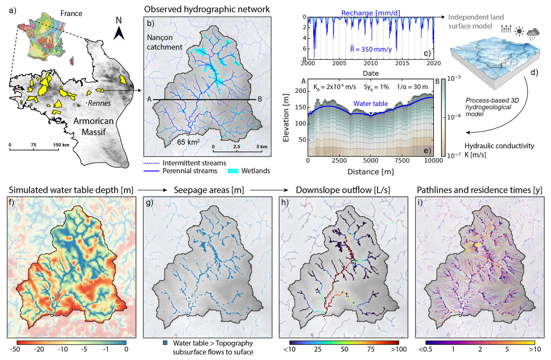
Figure 2 HydroModPy modeling steps illustrated for the Nançon catchment, Brittany (France). (a) Extraction of the watershed from a regional DEM, located to the west of the Geological Map of France. (b) Clip data based on the watershed extent. (c) Recharge time series provided from an independent land surface model. (d) 3D diagram illustrating the model conceptualization and parameterization based on data available and assumptions. (e) The cross-section (A–B) illustrates the vertical grid discretization and the resulting water table. The parameters include an exponential decay $\mathrm{1}/\mathit{\alpha }$ with depth from the maximum hydraulic conductivity K₀ and specific yield Sy₀ (%) in the first layer. (f–i) 2D map top-view visualization displaying spatial data and model results in steady state across the study area (left to right): water table depth, seepage areas, accumulated outflow, pathlines, and residence times.

The delineation procedure starts with a preprocessing step correcting hydrologically the DEM by filling all local depressions and/or removing flat areas (WBT.FillDepressions and/or WBT.BreachDepressions), ensuring a continuous downslope flow. From the corrected DEM, flow direction (WBT.D8Pointer) and flow accumulation (WBT.D8FlowAccumulation) rasters are generated, which are essential for catchment extraction (WBT.Watershed). To account for groundwater divides that may extend beyond topographic catchment boundaries, the additional buffer enlarging the model domain around the extracted catchments should be adjusted by the user based on aquifer depth, ensuring that longer groundwater flow paths are captured depending on context settings. The final catchment polygon, exported in shapefile format, is used to spatially subset all input datasets for the selected study site (Fig. 2b).

2.2 Model conceptualization and data import

The default conceptualization of the hydrogeological model is based on a parsimonious set of assumptions that simplify the representation of the subsurface flow system. First, the top of the model is defined by the topography, where the spatial discretization adopts the DEM resolution and is implemented as a regular structured mesh grid. The depth discretization is defined by the number of layers set by the user. By default, no-flow boundary conditions are applied to the sides of the modelled domain (contour of the buffered zone). Nevertheless, constant hydraulic head can be imposed at prescribed domain limits to represent boundary conditions imposed by an ocean, sea, lake, river, or by lateral groundwater inflows from adjacent aquifer systems. The model can be run in steady-state or transient mode. The temporal discretization is controlled by the recharge input data: a single time step corresponds to a steady-state simulation, whereas multiple time steps define a transient simulation. A homogeneous recharge across the catchment can be implemented with a simple time series of values, or as a spatially distributed field using raster, 2D matrix, or netCDF files. An optional function allows to adjust the temporal discretization of the recharge time step (e.g., daily to monthly). By default, recharge (Fig. 2c) is applied uniformly across model cells at the top of the water table.

HydroModPy includes functions to directly import data into the model domain area defined from the catchment delineation. Two main types of data are processed. (1) The data required to set up the hydrogeological model, including the aquifer's hydraulic properties, inputs, or boundary conditions, such as groundwater recharge (climatic.py) and sea level variations (oceanic.py) for coastal aquifers. (2) The data to constrain parameters and calibrate the model, including the piezometric levels (piezometry.py), streamflow rates (hydrometry.py), and the stream network (hydrography.py) with its intermittence (intermittency.py). All datasets are clipped to the model domain area (Fig. 2b), stored within a watershed Python-object, and then exported as time series (CSV) or georeferenced files (raster, shapefile, or netCDF) in the results folder. Furthermore, for applications in France, two automated functions are available to download climatic and piezometric data for the targeted study site via the APIs provided by Météo-France (Météo-France, 2025) and ADES (Winckel et al., 2022), respectively.

2.3 Aquifer parameterization

The initial step consists of parameterizing the aquifer geometry, followed by the assignment of its hydraulic properties. The model thickness may be defined as constant, assuming an aquifer base parallel to the topography with a uniform depth, or as spatially variable, with the aquifer base prescribed either as a single elevation value or as a spatially distributed elevation field (e.g., raster). The model thickness is discretized according to the number of layers set by the user. The thickness of the layers can be either constant or variable (e.g., increasing exponentially with depth). The hydraulic conductivity K and the storage coefficient S of the aquifer (specific yield Sy and the specific storage Ss) are by default taken as uniform and isotropic across the entire model domain. However, spatial heterogeneity can be readily incorporated by defining parameter zones based on geological maps or user-specified units. Vertical variability of hydraulic properties can be represented as a function of depth or stratigraphic layering, for example through an exponential decay of K, Sy, and Ss with depth (Fig. 2e). Anisotropy is treated separately as directional differences in conductivity (e.g., K_h≠K_v).

2.4 Computation of groundwater flow, particle tracking and transport

With its modular structure, HydroModPy is extensible and adaptable to various models and computational methods (Fig. 2d). The current groundwater flow solver is based on MODFLOW-NWT, a Newton–Raphson formulation of MODFLOW-2005 (Harbaugh, 2005; Niswonger, 2011) through the library FloPy (Bakker et al., 2016; Hughes et al., 2023) (modflow.py). This configuration is primarily suited for catchments where the hydrogeological boundaries roughly correspond to topographic divides, which typically corresponds to shallow unconfined aquifers.

Indeed, the modeling approach settings particularly contribute to quantifying groundwater–surface connectivity through the spatio-temporal simulation of baseflow and the associated dynamics of the hydrographic network. To achieve this, the fully convertible layer type of MODFLOW is applied: a cell is considered confined if the overlying cell contains groundwater, and unconfined otherwise. For an unconfined (resp. confined) layer, the storage coefficient corresponds to the specific yield (Sy) (resp. vertically integrated specific storage Ss). Seepage areas resulting from water table intersections with the topography (Anderson et al., 2015) are simulated thanks to the MODFLOW Drain (DRN) package applied at the model surface. In this configuration, seepage is not re-infiltrated into the aquifer but is instead considered as either surface runoff or direct contribution to streamflow. Additional packages can be activated to simulate other processes, such as the Streamflow-Routing (SFR) package, which enables the representation of more complex groundwater–surface water interactions, including losing stream conditions. When a user specifies a negative recharge input, the Evapotranspiration (EVT) package is automatically activated at the highest active cell (i.e., at the water table), with some options to define the extinction depth for evaporation. Nevertheless, the current version of HydroModPy focuses mainly on saturated groundwater flow, and unsaturated zone processes are not explicitly simulated. For coastal aquifers, constant hydraulic head boundary conditions can be imposed along the seaside limit of the model domain using the Constant-Head (CHD) package. Modeled cells with DEM elevation lower than the imposed hydraulic head are considered as fixed head boundary conditions.

Furthermore, HydroModPy integrates particle tracking through the MODPATH (modpath.py) suite (Pollock, 2012) to determine subsurface flow paths and associated residence times. Solute transport is implemented using the MT3DMS (mt3dms.py) suite (Bedekar et al., 2016), enabling simulation of single-species transport with advection, dispersion, and diffusion. Basic reaction processes are supported through zero-order and first-order degradation kinetics (e.g., for conservative or moderately reactive solutes such as nitrate). Heterogeneous initial concentration distributions can be specified. More advanced reactive transport and multi-species configurations are envisioned as future extensions.

2.5 Standardized outputs and visualization capacities

HydroModPy stores input data, model parameters, and simulation results in standard formats. From a single user-specified path, the results are automatically saved in a designated directory. Two main folders are generated: “results_stable”, which contains data collected from the study site at the scale of the model domain, and “results_simulations”, which contains hydrogeological simulation outputs. All data, whether inputs or outputs, adhere to standard file formats – CSV (.csv), raster (.tif), shapefile (.shp), netCDF (.nc), and VTK (.vtk) – to facilitate their use in external tools such as QGIS (QGIS Development Team, 2024) or ParaView (Ahrens et al., 2005) for visualization. This architecture ensures seamless analysis and consistent interpretation of hydrogeological model outputs across different sites and simulation scenarios. It also provides a significant advantage when comparing HydroModPy results with outputs from other hydrological models. Additionally, to ensure a FAIR approach, all input data and model parameters are recorded in a metadata file. This file tracks the complete model parameterization, facilitating reuse for further analyses and avoiding the need to recompute watershed information. As a result, new hydrogeological models with different parameterizations can be run more efficiently.

Spatio-temporal simulation outputs include water table elevation, water table depth, groundwater flow and storage. For the interactions with the land surface, outputs include groundwater discharge at the surface (outflow), and the associated patterns of seepage areas (Fig. 2f–i). From these seepage cells, a continuous hydrographic network is derived by routing and accumulating groundwater discharge along the steepest topographic gradient (downslope.py). The resulting network represents stream reaches sustained by groundwater discharge and can therefore be used to investigate spatial and temporal variations in stream network extent associated with changes in baseflow conditions.

Visualization of data and model results leverages the Matplotlib library (Hunter, 2007) (visualization_watershed.py and visualization_results.py) for graphs and 2D maps, and the Vedo library (Musy et al., 2022) for 3D representations using generated VTK files (export_vtuvtk.py). In 2D top-view, users can map the location of the watershed within the initial DEM using visualization_watershed.watershed_local and visualize the watershed topography with visualization_watershed.watershed_dem. Additionally, catchment characteristics and model results can be mapped (Fig. 2e–i) using the visualization_results.visual2D function. This includes the topography and model grid, water table elevations and depths, seepage areas, and the associated accumulated surface flow. If particle tracking has been enabled, outputs also include the starting and ending locations of injected particles, as well as subsurface pathlines with their associated residence times. Interactive exploration of water table levels at each model point is possible through the visualization_results.interactive_cross_section tool. Similarly, the visualization_results.visual3D function provides interactive 3D representations of the features listed above using VTK files and the Vedo package.

3 Applications

3.1 Current global case studies

To date, HydroModPy has been used to model a wide range of catchments across the world. The regions most frequently studied are mainly characterized by shallow aquifers (brown areas on the hydrogeological map in Fig. 3) (Taylor et al., 2013; Richts et al., 2011), underlain by relatively low-permeability lithologies, such as crystalline bedrock. A broad range of research and applied questions have been addressed, including (1) the management of water resources, (2) the understanding of groundwater flow or transport processes, and (3) the development of innovative tools and their integration with existing ones. These 3 main categories are presented below.

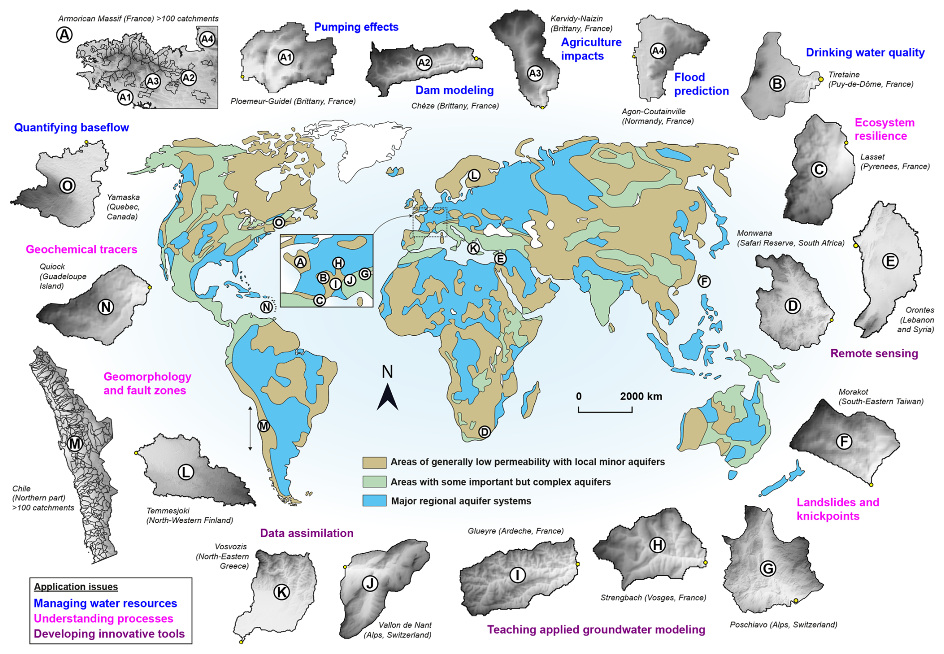
Figure 3 Worldwide application sites of HydroModPy. Simplified global groundwater resources map, modified from Taylor et al. (2013) and originally obtained from Richts et al. (2011). Catchments are grouped into three main application fields: water resources management, process understanding, and tool development. Since HydroModPy primarily focuses on subsurface–surface interactions, all catchments are located in areas of generally low permeability with shallow, local, minor aquifers (brown areas on the world map). Extensive applications of HydroModPy have been carried out in France (A) and Chile (M) across multiple catchments.

1. HydroModPy has already been used to build groundwater models addressing water resource management challenges, such as the impacts of well pumping on groundwater flow at the catchment scale (Fig. 3A1), the influence of dams on surface–subsurface interactions (Boivin et al., 2025, Fig. 3A2), and the effects of agricultural practices on pollutant legacy in groundwater (Bagagnan et al., 2026). It has also been applied to flood forecasting in connection with groundwater dynamics (Gauvain, 2022; Le Mesnil et al., 2026, 2024, Fig. 3A4), the assessment of headwater resources availability for drinking water (Aumar et al., 2024, Fig. 3B), and the estimation of baseflow for groundwater-dependent ecosystems (Touzeau et al., 2025; Abhervé et al., 2025).

2. The efficient framework developed enhances our understanding of coupled groundwater flow and transport processes by enabling users to easily test various configuration settings and calibrate models using diverse datasets. For instance, the toolbox has been successfully applied to calibrate models using geochemical tracers (Gaillardet et al., 2025, Fig. 3N). Recent studies have also explored geomorphological controls on spatio-temporal groundwater discharge, including the role of fault zones in surface-subsurface connectivity (Marti et al., 2025, Fig. 3M), the contribution of groundwater to slope instabilities inducing possible landslides (Steer et al., 2024, Fig. 3F), and the effect of knickpoints on groundwater dynamics (Floriancic et al., 2024, Fig. 3G).

3. Finally, new tools have emerged in HydroModPy and can be integrated with existing ones. The platform provides a valuable resource for teaching applied physically-based groundwater modeling in academic and professional contexts (Fig. 3H, I). It can be connected to data assimilation approaches (Fig. 3J, K), used with approximate scientific computing methods (Sallou et al., 2020, Fig. 3A4), and combined with remote sensing datasets to enhance hydrogeological modeling capabilities (Fig. 3D, E).

Through these diverse applications, HydroModPy demonstrates its versatility as both a scientific and operational tool, addressing key challenges in water resources management, process understanding, and methodological innovation. While HydroModPy can be used in several contexts to answer various scientific questions, it has been primarily developed to facilitate the automatic deployment of catchment-scale groundwater models with unconfined aquifers. Regional-scale deployments have been carried out in France (Fig. 3A) and Chile (Marti et al., 2025, Fig. 3M), to simulate and calibrate hundreds of headwater catchment models. These works demonstrate the tool's capability to repeat a calibration methodology across multiple catchments using available data, as illustrated by the application in Sect. 3.2.

3.2 Example of a calibration method deployment

Following the approach of Abhervé et al. (2023, 2024), we use HydroModPy to constrain aquifer hydraulic properties based on stream network maps and streamflow intermittence, demonstrating particular effectiveness for ungauged basins. The objective is to illustrate how HydroModPy can be systematically employed to set up, simulate, calibrate, and analyze hydrogeological models across multiple catchments, with calibration primarily targeting catchment-scale effective hydraulic properties. Thanks to its streamlined workflow, the methodology can be implemented with only a few lines of code, as illustrated in conceptual Fig. 4. In the presented example, a for loop (Line 8 in Listing 4) is used to iterate over the outlet coordinates of 31 catchments (Line 6 in Fig. 4), enabling automatic model construction, parameter assignment, simulation execution, and generation of model outputs. In this section, we apply a similar calibration approach to further refine the hydraulic properties of the studied catchments. Note that other examples, including all required input data and expected outputs, are provided as fully executable Jupyter notebooks in the HydroModPy documentation at https://docs.hydromodpy.fr/v1.0/examples.html (last access: 4 July 2026), enabling users to immediately replicate and adapt the workflow to their own study areas.

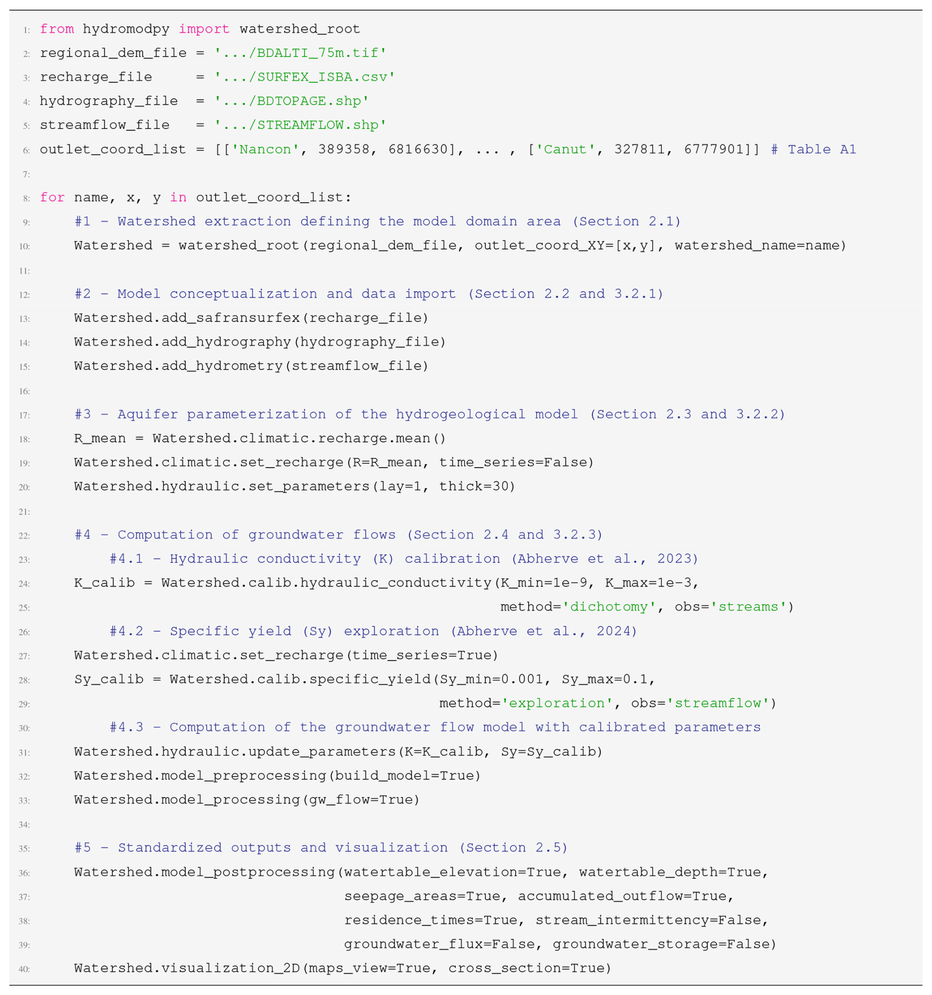
Figure 4 Example of a conceptual python code for running a model with HydroModPy on two different catchments (Nançon and Canut).

3.2.1 Study sites and datasets

The 31 catchment areas are located in the western Armorican Massif, France (Figs. 2a and 3A). Their outlet coordinates are specified in Table A1 in the Appendix. The catchments were selected based on the availability of perennial/intermittent stream network maps and streamflow data measured at the catchment outlets. The catchments were initially extracted from the DEM (Line 2 and 10 in Fig. 4) of the BD ALTI^® (IGN, 2011). Aquifer recharge R (Line 3, 13, 18 and 19 in Fig. 4) is derived from the independent land surface model SURFEX (SAFRAN-ISBA), which solves the energy and water fluxes at the soil–vegetation–atmosphere interface over the French metropolitan area at a spatial resolution of 8 × 8 km² (Le Moigne et al., 2020; Météo-France, 2025, Fig. 2c). The datasets used to constrain the models are mostly open data and include stream network maps (Line 4 and 14 in Fig. 4) from BD TOPAGE for “hydrography” (IGN, 2020, Fig. 2b), absence/presence of water in streams from ONDE for stream “intermittency” (Nowak and Durozoi, 2012, Fig. 2b), and streamflow rate data (Line 5 and 15 in Fig. 4) from Hub'Eau for “hydrometry” (Dequesne and Portela, 2024). Catchment areas range from 7 (Langelin) to 526 km² (Hyeres). The dominant lithology of the catchments is primarily composed of plutonic rocks (granite), Brioverian schists, or Paleozoic sandstones (BRGM, 2006).

3.2.2 Model setup

For the 31 study sites, the model resolution is determined by the 75 m resolution of the DEM. The top of the aquifer is defined by the land surface topography, while the bottom is set at 30 m below ground level (Line 20 in Fig. 4), with only one layer. This thickness represents the typical depth of the interface between the shallow weathered and/or fractured zone with the underlying fresh bedrock (Roques et al., 2016; Kolbe et al., 2016; Dewandel et al., 2006; Mougin et al., 2015). This approach primarily assumes lateral, near-surface groundwater flow following the topography. Thus, across all catchments, the number of grid cells ranges from 2800 to 207 152 (Table A1). The conceptualized shallow and uniform aquifer thickness represents the typical depth of the transmissive and weathered and/orfractured zone of the crystalline bedrock in the Armorican Massif. The aquifer is assumed to be isotropic and homogeneous, characterized by uniform effective hydraulic properties at the catchment scale: hydraulic conductivity (K) and specific yield (Sy). Recharge is applied uniformly across the model domain. The model is first run in steady-state, followed by transient simulations conducted over a three-year period with monthly stress periods.

3.2.3 Calibration approach

The hydraulic conductivity K is first constrained (Line 24 in Fig. 4) on the observed perennial stream network (BD TOPAGE, IGN, 2020). The simulations are run in steady state with a mean recharge (Lines 18 and 19 in Fig. 4). Using a dichotomy approach with initial K values between 10⁻⁹ and 10⁻³ m s⁻¹ (Fig. 5a) (Domenico and Schwartz, 1998; Freeze and Cherry, 1979), the model minimizes the mismatch distance between the simulated and the observed stream network (Abhervé et al., 2023). In the objective function, D_SO denotes the average distance from the simulated stream network cells to the nearest downslope observed stream network (Fig. 5b), while D_OS represents the reverse (Fig. 5c). The optimal simulation is obtained when $\stackrel{\mathrm{‾}}{D_{\mathrm{OS}}}$=$\stackrel{\mathrm{‾}}{D_{\mathrm{SO}}}$. The distance D_optim is defined as the average of $\stackrel{\mathrm{‾}}{D_{\mathrm{SO}}}$ and $\stackrel{\mathrm{‾}}{D_{\mathrm{OS}}}$. The smaller the value of D_optim, the better the match of the simulated seepage pattern and the observed stream network.

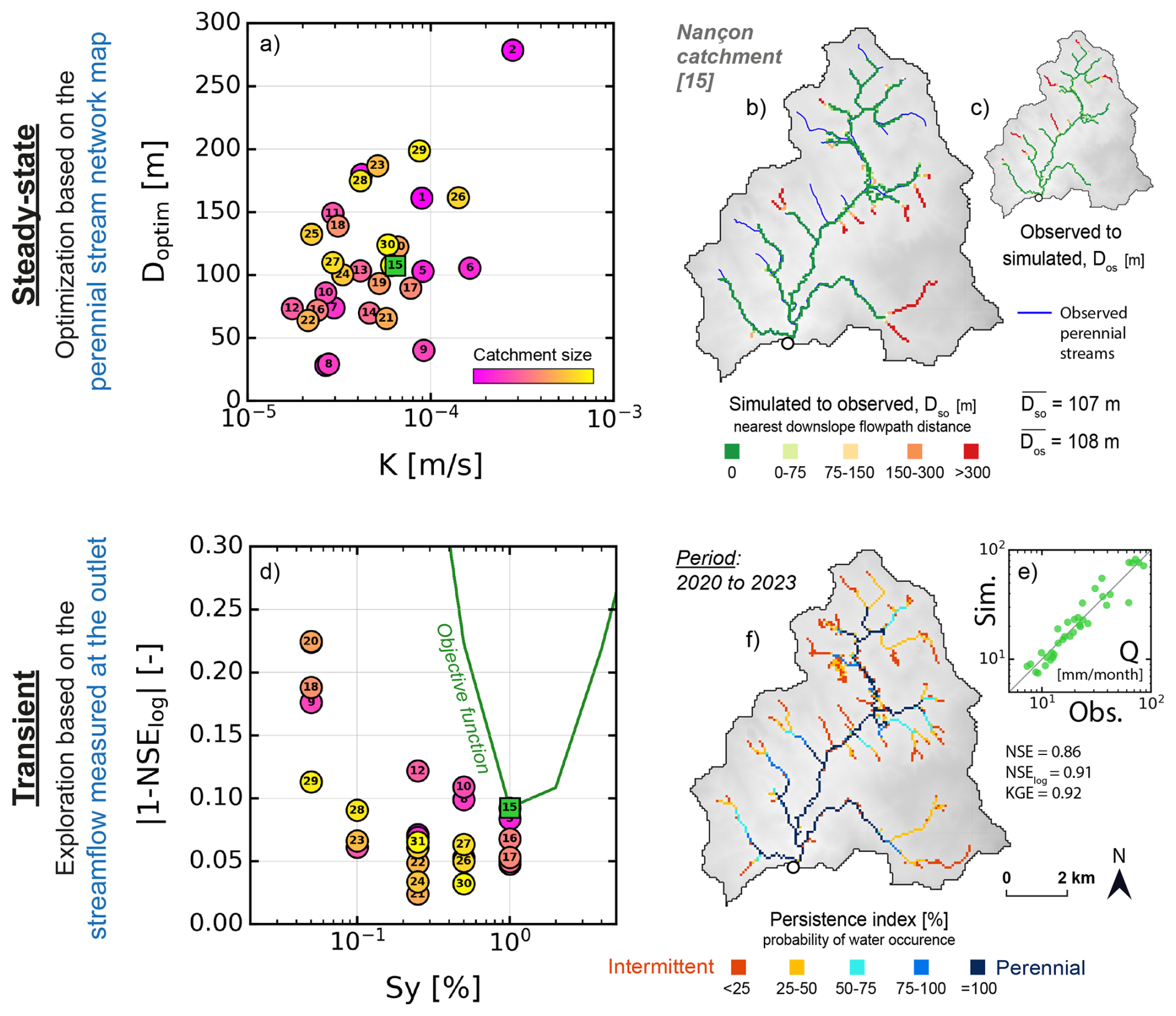
Figure 5 Calibration results for the estimation of hydraulic conductivity K and specific yield Sy for 31 catchments: (a) The best value of hydraulic conductivity K versus D_optim. The color bar represents relative catchment size. The green square highlights the Nançon catchment. (b) Simulated hydrographic network showing the distance D_SO from simulated seepage pixels to the nearest downslope observed stream network. (c) Similar representation for D_OS. (d) The best value of specific yield Sy obtained for each catchment versus the associated $|\mathrm{1}-NS{E}_{\text{log}}|$ criterion. The green line represents the objective function of the Nançon catchment. (e) Comparison of observed and simulated specific streamflow at the catchment outlet Q. The black line indicates the 1:1 relationship. (f) Representation of the persistence index of the simulated results, showing maximum (orange lines, highly intermittent) and minimum (dark blue lines, perennial) extents of the simulated stream network.

The specific yield Sy is then calibrated in transient state (Lines 28 and 29 in Fig. 4) by comparing the simulated streamflow at the catchment outlet with the measured data. Using Nash and Sutcliffe Efficiency criteria at logarithmic scale to focus on baseflow (Nash and Sutcliffe, 1970; Oudin et al., 2006) (Fig. 5e), the optimal model is selected from a set of 10 candidate values of specific yield (Sy), regularly spaced and independently evaluated for each catchment, within the range of 0.1 % to 10 % (Fig. 5d). The consistency of stream intermittency, represented by the persistency index across the catchment (Fig. 5f), is used to validate the model’s ability to accurately simulate spatio-temporal patterns of stream expansion/contraction. At the end, a transient simulation over the 3-year period with the estimated parameters is run (Lines 30 to 33 in Fig. 4).

3.2.4 Results and interpretation

Some functions are used to assess the simulation results (Lines 36 to 40 in Fig. 4). The visualization tools allow to easily display calibration performance criteria (Fig. 5a and d), the simulated perennial stream network (Fig. 5b and c), the stream intermittency map (Fig. 5c), and the comparison between simulated and measured streamflow at the outlet.

Calibration is acceptable for all catchments with D_optim values less than 300 m (4 times the DEM resolution) and NSE_log values greater than 0.75 (Fig. 5a–d), indicating a good fit between simulated and observed stream networks and streamflow, respectively. By automating the modeling process through Python scripts, the workflow is significantly streamlined, enabling the systematic and reproducible calibration of effective hydraulic conductivities K and specific yields Sy. The successful deployment of HydroModPy across 31 catchments with various sizes demonstrates the scalability and robustness of the approach. Consistently high model performance across the range of hydrological settings, catchment sizes, and topographic contexts represented within the Armorican Massif dataset confirms the reliability of the simplified conceptual framework and automated calibration methodology. This systematic implementation demonstrates HydroModPy's scalability across catchment sizes within its targeted scope of shallow, unconfined, and topography-controlled groundwater systems, providing a standardized and efficient framework for comparative analyses using widely accessible datasets.

As an example at a pilot site, the Nançon catchment (67 km², 27 004 cells, Fig. 2b) has an estimated K of $\mathrm{6.40}\times {\mathrm{10}}^{-\mathrm{5}}$m s⁻¹, with a consistent representation of the perennial stream network (Fig. 5b–c). This value is consistent with the lithological context (Domenico and Schwartz, 1998; Freeze and Cherry, 1979; Gleeson et al., 2011) and aligns with local measurements (Dewandel et al., 2021). A specific yield of 1 % is calibrated on the observed streamflow at the outlet, with a NSE_log equal to 0.91 (Fig. 5e). The overall close agreement between stream intermittency (Persistence index, Fig. 5f) and simulations confirms the model's ability to correctly represent groundwater dynamics and the surface-subsurface interactions at the catchment-scale.

4 Discussion

HydroModPy has been developed to address the growing need for deployable modeling tools capable of simulating groundwater flow and solute transport at the catchment scale, with a strong emphasis on accessibility and ease of use. As an open-source toolbox, HydroModPy provides a user-friendly, flexible, and adaptable platform for modeling hydrogeological systems across a wide range of spatial scales (typically from 1 to 10³ km²). The toolbox enables the development of efficient and reproducible modeling workflows across multiple sites using straightforward Python scripts. Its modular and extensible architecture allows users to tailor and expand its functionalities to address specific research objectives or practical applications. This versatility opens up new opportunities to investigate hydro(geo)logical processes across diverse environmental and management contexts. In the following sections, we discuss the identified strengths and limitations of HydroModPy, outline ongoing developments and future directions, and emphasize its value as a pedagogical tool for teaching hydrogeological modeling.

4.1 Strengths and limitations of current examples

The tool deployment across 31 catchments in Brittany and Normandy highlights several key strengths. First, the automated workflow successfully calibrated all models with consistent performance metrics (NSE_log>0.75), demonstrating robust convergence across a range of catchment sizes (7–526 km²) within a relatively homogeneous crystalline basement context. The calibrated effective hydraulic conductivity values ($\mathrm{1.75}\times {\mathrm{10}}^{-\mathrm{5}}$ to $\mathrm{2.79}\times {\mathrm{10}}^{-\mathrm{4}}$ m s⁻¹) are relatively similar among catchments, which is consistent with the shared geological setting and with values reported in the literature for crystalline basement aquifers (Lachassagne et al., 2021). Second, the standardized modeling framework enables systematic comparisons across regions while preserving local specificity. The consistency of calibrated parameters among neighboring catchments with similar geological contexts further validates the reliability of the methodology. This approach offers a scalable solution for comparative hydrogeological analysis across multiple catchments, within the current scope of shallow unconfined aquifers where topographic divides approximate hydrogeological boundaries. It is worth noting that HydroModPy supports a buffer-based domain extension to capture potential inter-catchment groundwater exchanges, and model boundaries can also be defined manually via shapefiles to accommodate cases where surface and groundwater divides diverge. Third, HydroModPy’s ability to integrate multiple data sources, when these datasets are available for the catchments of interest, substantially reduces the time and technical barriers typically encountered in catchment-scale groundwater modeling. In practice, successful integration still depends on the user verifying data availability, completeness, and quality for each study site.

Despite its demonstrated capabilities, current examples presented in this study and default options of HydroModPy present certain limitations, mostly related to its targeted scope of applicability. In the presented results, the tool is primarily designed for shallow, unconfined aquifers and topography-controlled groundwater systems, where surface catchment boundaries approximate groundwater divides. This underlying assumption may not hold in the case of deep confined aquifers, karst systems, or regions with significant inter-basin groundwater exchanges (Le Mesnil et al., 2020). The current conceptual model employs several simplifications that improve usability but limit its straightforward applicability in complex and highly heterogeneous hydrogeological settings. The omission of unsaturated-zone processes means that recharge is transmitted directly to the water table, potentially overestimating the groundwater response to precipitation events. Additional, more easily addressable limitations include the default assumption of homogeneous effective hydraulic properties within each catchment, which may fail to capture the heterogeneity typical of geological contacts or stratified aquifers. The instantaneous surface routing scheme neglects key processes influencing surface – subsurface interactions, such as reinfiltration. Finally, the assumption of spatially uniform recharge cannot capture variations in precipitation, evapotranspiration, land cover, or land use-factors that must be considered when addressing specific scientific questions and hydrological challenges.

Beyond structural simplifications, uncertainty and equifinality represent important methodological considerations that are not yet explicitly addressed in the current calibration framework. In particular, multiple parameter combinations may produce equally acceptable model fits which can limit the interpretability of calibrated values and the robustness of model predictions. Uncertainty in input data (e.g., recharge estimates, stream network maps) and model structure further compounds this issue.

However, it is important to note that many of these limitations can be overcome by making use of HydroModPy's advanced functions and modular structure. For instance, to address heterogeneity and geological complexity, future developments could enable the integration of a 3D geological model during the parameterization stage. Likewise, additional processes can be incorporated by activating specific MODFLOW packages, such as the evapotranspiration (EVT) or streamflow routing (SFR) modules, thereby extending the framework's applicability to a wider range of hydrogeological contexts.

4.2 Improvements and perspectives

One of the primary objectives of the collaborative platform HydroModPy is to create long-term opportunities to advance hydro(geo)logical modeling by integrating processes across the critical zone and coupling them with emerging tools and datasets. Future developments aim to further enhance its ability to simulate surface and subsurface hydrodynamics with improved computational efficiency and, where necessary, greater process complexity. Another planned development is to dissociate the model grid resolution from the resolution of the input DEM. In the current version, the DEM resolution defines the model grid, whereas future versions aim to allow these two resolutions to be specified independently, providing greater flexibility to balance topographic detail, model design, and computational cost. The framework is designed to interface with other simulators capable of modeling subsurface flow. Its flexible architecture enables integration with a range of hydro(geo)logical models, such as HS1D (Marcais et al., 2017) and the updated MODFLOW 6 (Langevin et al., 2017). In this sense, a specific integration of MODFLOW 6 via its Application Programming Interface (API, Hughes et al., 2022) is also currently under development. HydroModPy’s expanded couplings will enhance its modeling capabilities by providing users with additional tools to simulate complementary hydrogeological processes aligned with their specific research objectives. Furthermore, integrating multiple groundwater flow solvers within a unified HydroModPy framework will enable robust model intercomparison and benchmarking, thereby supporting more comprehensive analyses and facilitating the selection of the most appropriate modeling approach for a given hydrogeological study or application. A major ongoing development is the integration of other open-source codes to represent additional components of the water cycle, such as exchanges with the atmosphere and interactions within the plant–air–soil continuum (e.g., ecohydrological models). Land surface models will also improve the representation of groundwater recharge inputs. Currently two land surface models are under implementation in HydroModPy: the rainfall-runoff model GR4J (Génie Rural à 4 paramètres Journalier) (Perrin et al., 2003), and the distributed Hydrologic Evaluation of Landfill Performance model (HELP) (Croteau et al., 2010). Distributed land surface models will allow users to include spatially variable climate data, soil characteristics, and land use information in their simulations, enabling the calculation of spatio-temporal groundwater recharge rates relevant from hillslope to regional scales. These couplings can be implemented sequentially between groundwater flow solvers and unsaturated zone processes, including interactions among the water table, soil moisture, and evapotranspiration, as well as the associated feedback mechanisms. Through these developments, along with the addition of new functions and code modules to represent greater complexity or new processes, we aim to extend HydroModPy’s applicability to a broader range of hydrological contexts (e.g., confined aquifers, alluvial plains, or settings where the unsaturated zone plays a critical role). Ultimately, this approach will enable users to select the most appropriate processes, level of complexity, and functions based on their knowledge of the study site and its underlying conceptual model.

Downloading data for a catchment area is often a time-consuming step in environmental science studies. It is also one of the most tedious stages in hydrogeological modeling. In this context, one of the main goals of the HydroModPy community is to incorporate and develop new tools for downloading and importing both observed and modeled data for the spatial extent of the target model. We currently provide this functionality for piezometry and climate data in France (see Sect. 2.2), but we plan to connect it to larger and more comprehensive databases worldwide.

At a global scale, for instance, we can cite resources such as Caravan (a series of CAMELS: Catchment Attributes and Meteorology for Large-sample Studies) (Kratzert et al., 2023), GRDC for the Global Runoff Data Centre (https://grdc.bafg.de/, last access: 4 July 2026), or ERA5 for climate information (Hersbach et al., 2023). We plan to progressively develop connectors to these and other global data sources, prioritizing resources based on API maturity, data licensing terms, and community demand. Once implemented, these connectors will enable users to directly harvest diverse datasets (topography, geology, land cover, water use, etc.) relevant to their specific modeling objectives. This approach illustrates the tool’s capacity to leverage widely accessible data, thereby enhancing reproducibility and promoting broader adoption within the hydrological community.

Thanks to the scriptable and user-friendly design of HydroModPy, the current calibration strategy primarily relies on systematic parameter exploration (Fig. 5d) using goodness-of-fit metrics such as NSE (Nash and Sutcliffe, 1970), RMSE, and KGE across multiple datasets. Classical hydrogeological modeling typically uses data such as groundwater head measurements, but as previously discussed, surface water data (e.g., streamflow rates) and, more innovatively, stream network mapping following the approach of Abhervé et al. (2023) are also incorporated. In addition to the dichotomous calibration approach used in this study (Fig. 5a), ongoing developments aim to implement more sophisticated optimization-based calibration techniques, including optimization algorithms such as the Simplex method (Nelder and Mead, 1965) and the Metropolis–Hastings algorithm (Hastings, 1970). In parallel, tailored calibration strategies are being developed to address specific modeling objectives. Future plans also include integrating established open-source tools for parameter estimation and uncertainty analysis, such as pyEMU (White et al., 2016), which builds on PEST (Doherty, 2015). These developments will also address the equifinality challenge inherent in catchment-scale groundwater model calibration, by enabling formal uncertainty quantification and the identification of parameter sets that are non-uniquely constrained by the available observations. These advancements will support multi-criteria, multi-observable, and multi-method calibration, providing a more robust, automated, and comprehensive framework for hydrological model optimization.

In addition, HydroModPy is being enhanced with a user-friendly interface, notably through the development of a graphical environment using Jupyter Notebook widgets (Kluyver et al., 2016). This improvement is designed to provide users with an intuitive and interactive platform for model setup, execution, and visualization, thereby streamlining the modeling workflow and enhancing the overall user experience. Tools such as Voilà (de Marchi, 2021) or the web-based platform Galaxy (Hiltemann et al., 2023) could further support the creation of customized graphical interfaces and facilitate their manipulation. These developments will ultimately increase HydroModPy’s accessibility and usability, making it a valuable tool not only for researchers but also for water resource managers and other stakeholders.

4.3 Suitability for teaching groundwater modeling

HydroModPy provides a new opportunity for training and teaching applied hydrogeological modeling. By enabling the simulation of physically based groundwater flow models it complements the capabilities already offered by conceptual rainfall–runoff models such as GR4J (Delaigue et al., 2023) and HBV (Seibert and Vis, 2012). We believe that HydroModPy is particularly well suited for Master-level courses and has already been taught at three universities in France and Switzerland: the University of Rennes, the University of Grenoble, and the University of Neuchâtel. In line with modern teaching methods, HydroModPy is implemented in a Jupyter Notebook, allowing users to run the toolbox with Python. These interactive notebooks enable students to engage with the modeling process in a structured, step-by-step manner, allowing them to run models that explicitly represent groundwater flow or transport using just a few lines of code. Another advantage of this approach is that it provides a continuously evolving platform for education, as the scripts and notebooks can be easily adapted to new topics or datasets. HydroModPy-based teaching scripts have already been successfully used by environmental science students, demonstrating their accessibility and ease of use, even for beginners in programming and hydrogeological modeling. Students can develop their own catchment-scale MODFLOW models, enabling them to focus directly on both fundamental and applied questions, such as investigating the influence of hydrogeological parameterization and boundary conditions on simulations. The main advantage is that students can quickly focus on a specific scientific topic, such as exploring the influence of climate or geology on groundwater flow partitioning and its indirect impact on the connectivity of surface water networks at the catchment-scale. By integrating HydroModPy into the academic curriculum, students gain hands-on experience in hydrogeology-specific modeling techniques, programming, data analysis, and result interpretation. Georeferenced outputs can be directly visualized in GIS tools, such as QGIS (Graser et al., 2025) providing an interactive way for students to explore and compare spatio-temporal simulation results. Thanks to its visualization tools, HydroModPy-based courses can dynamically illustrate how hydrological systems respond to changes in model parameters, such as topography, aquifer geometry and thickness, hydraulic conductivity, porosity, or recharge. More broadly, students can test different perturbation scenarios on groundwater systems – for example, implementing pumping at any chosen location, forcing the model with future climate change scenarios (e.g., CMIP climate projections, Copernicus Climate Change Service, Climate Data Store, 2021; O'Neill et al., 2016), or a combination of both.

5 Conclusions

HydroModPy is a comprehensive Python toolbox for constructing, calibrating, and analyzing catchment-scale shallow groundwater models in a systematic and reproducible manner. By integrating geospatial analysis, hydrogeological modeling, and standardized visualization within a unified framework, HydroModPy overcomes the technical barriers that have traditionally limited the deployment of groundwater models across multiple sites and scales. Its successful application across 31 catchments demonstrates the toolbox’s ability to systematically calibrate hydrogeological models using widely accessible datasets. All models achieved consistent performance metrics, with calibrated effective aquifer hydraulic properties values aligning well with independent hydrogeological studies. This validation confirms both the physical plausibility of the results and the robustness of the automated workflow across diverse catchment scales.

The modular architecture of HydroModPy facilitates the transition from localized, detailed studies to regional-scale assessments through standardized procedures. By automating watershed delineation, data retrieval, model construction, and result visualization, the toolbox significantly reduces the time and expertise required for hydrogeological modeling while maintaining scientific rigor. Integration with established tools, such as WhiteboxTools and FloPy-MODFLOW, ensures reliability, while standardized output formats (CSV, raster, shapefile, netCDF) promote interoperability and adherence to FAIR principles. Moreover, relying on collaborative development, HydroModPy’s design allows for the easy integration of new functionalities, the coupling of the currently integrated MODFLOW model with other simulators, and the incorporation of additional codes into the existing framework.

Beyond its technical capabilities, HydroModPy provides significant educational and community benefits. Its user-friendly Python scripts, Jupyter Notebook interface, and interactive visualization tools make complex hydrogeological concepts accessible to students and non-specialists, while its open-source nature fosters collaborative development and knowledge sharing.

In a context where the hydrological community increasingly emphasizes reproducible science, open-source solutions, and interdisciplinary collaboration, HydroModPy helps democratize access to advanced modeling capabilities without compromising scientific rigor. Within its current scope of shallow, unconfined, topography-controlled groundwater systems, the toolbox provides a practical link between detailed site-specific investigations and hillslope- to regional-scale water management needs, supporting evidence-based decision-making in an era of growing climatic uncertainty and environmental pressures. Future developments will aim to extend its applicability to more complex geological contexts, including multi-layered and confined systems, thereby broadening the range of hydrogeological assessments it can support.

Appendix A

Table A1 Calibration performance criteria for the 31 calibrated models including the watershed name, outlet coordinates in the Lambert93 reference system (EPSG:2154), watershed area, and number of model cells. The computation time (minutes), calibrated values and calibration criteria (D_optim and NSE_log) are shown for hydraulic conductivity K and specific yield Sy. Performances of calculations are given in computation times (minutes) on an Intel^® Xeon^® CPU E5-1620 v3 @3.50 GHz (4 cores, 8 threads) processor.