Validation of the open-source hydrodynamic model SFINCS on historical river floods at the global scale

We evaluate the performance of the Super-Fast INundation of CoastS (SFINCS) hydrodynamic model for simulating riverine floods, combined with a fully automated open-source data preprocessing pipeline. To do this, we assessed the simulated extent of 499 historic flood events against the satellite derived flood extents using the Critical Success Index (CSI) as a performance metric. We utilised simulated discharges from the Global Flood Awareness System (GloFAS) hydrological model and found that SFINCS performance improved with upstream basin size, with a global mean CSI of 0.42 for basins with large upstream area (>1000 km²) and a CSI of 0.29 for basins with small upstream area (<50 km²). Our results illustrate the importance of accurate discharge data input to flood hazard simulations. When the (globally simulated) GloFAS data is replaced with observed discharge data for ten events in the US, the CSI improved from 0.39 to 0.67. These results suggest that global hydrological model performance limits the accuracy of the flood hazard simulations. Our findings also showed a significant improvement in the CSI (from 0.37 to 0.57) when changing to a higher-resolution elevation input by contrasting a ∼1 m digital elevation model (DEM; 3DEP) with our default ∼30 m global DEM (FABDEM) in six US events. Sensitivity analysis of bathymetric calculations revealed a systematic underestimation of the default 2-year return period estimated by GloFAS discharge, likely driven by underrepresentation of annual block maxima, which resulted in underestimated channel dimensions. All of these factors resulted in a loss of detail, which impacted model performance, especially in smaller headwater rivers. We recommend to improve the estimation of bathymetry, for instance by employing the “gradually varying solver” method or using data from the SWOT mission. Furthermore, incorporating additional validation data which ideally includes flood depth measurements can largely enhance our understanding of the model performance.

1 Introduction

Riverine floods pose a significant global challenge, which makes their assessment crucial for designing effective flood management strategies that reduce flood damage and fatalities (Merz et al., 2021). Over the past decades, flood inundation modelling has become an important tool for assessing flood hazard and supporting flood managers in prioritising interventions to reduce risk (Teng et al., 2017). These modelling efforts often involve using hydrological forcings in hydrodynamic models to simulate water movement. These models usually solve equations derived from physical laws of fluid motion to produce flood extent and depth maps (e.g. Guo et al., 2021). However, other approaches exist, such as using machine learning (Nevo et al., 2022).

While the use of local-scale hydrodynamic flood models is a well-established approach for mapping flood hazard and assessing flood risk, large-scale or global inundation modelling still faces several challenges, such as topography and bathymetry data, computational intensity, and open accessibility of data (Wing et al., 2020; Wing et al., 2021; Dottori et al., 2022). For example, in recent years, several high-resolution global topography datasets have become available (Hawker et al., 2022; Abrams et al., 2020; Copernicus DEM, 2022), with increasing accuracy. Nevertheless, this data is too coarse to include river flood defences (Wing et al., 2019). Another significant challenge is the lack of open, high-resolution bathymetry data (Hawker et al., 2018). While river-width data has become available for rivers wider than 30 m (Allen and Pavelsky, 2018), data on river depth is still missing.

Furthermore, the computational demand to run large-scale models is high (Leijnse et al., 2021). Two-dimensional hydrodynamic models, such as the state-of-the-art global LISFLOOD-FP model, offer high detail but at a substantial computational cost (e.g. Wing et al., 2021; Bates, 2023). The computational intensity at the global scale has led to different modelling simplifications (e.g. Winsemius et al., 2015; Van Ormondt et al., 2025) and the development of novel computational approaches using graphic processing unit (GPU) architecture (Shaw et al., 2021; Apel et al., 2024). Lastly, not all parts of the code for setting up global flood models are open-source, which limits comparability and reproducibility (Hall et al., 2022; Hoch and Trigg, 2019).

Due to these challenges, there is growing interest in open-source hydrological and hydrodynamic models (e.g. HEC-RAS; Zeiger and Hubbart, 2021) that are easily applicable to data-scarce regions and computationally efficient (Kim et al., 2019). One such model is the Super-Fast INundation of CoastS (SFINCS) model (Leijnse et al., 2021), which has shown promise in coastal and compound flooding scenarios (Eilander et al., 2023b; Nederhoff et al., 2024) but can also be applied to fluvial and pluvial flooding. SFINCS achieves fast computational speeds by simplifying dynamic flow equations and using efficient spatial discretisation techniques with a subgrid (Leijnse et al., 2021). Another key advantage of the SFINCS model is that it is fully open-source, alongside (Python) packages to preprocess the data (Eilander et al., 2023a).

Although the SFINCS model has demonstrated high performance in modelling compound floods in coastal areas at both small and larger scales (e.g. Leijnse et al., 2021; Benito et al., 2024), its performance for riverine floods has not yet been investigated. Understanding how SFINCS performs for riverine floods, particularly at large scales and across different parts of the world, is important, especially due to the aforementioned challenges related to input data and model simplifications. Validation plays a key role in understanding model reliability, especially for flood hazard models applied at continental to global scales (Ward et al., 2013; Bates, 2023). However, global data for model validation, such as flood extent observations (e.g. Sampson et al., 2015), are scarce, with most large-scale studies lacking extensive validation against real flood events. Instead, these studies have often focused on producing flood hazard maps for several return periods (e.g. Dottori et al., 2022) and benchmarking these simulations against other national and regional engineering models (e.g. Wing et al., 2024). Studies conducting event-based validation have not been global in scale, or they have focused on a limited number of events (e.g. Risling et al., 2024, validating eight flood events across large river basins on four continents; Wing et al., 2021, using 35 events in the United States; Bernhofen et al., 2018, using two events in Nigeria and Mozambique).

In the last decade, the use of satellite imagery has become an increasingly popular source for validating flood hazard models (e.g. Bernhofen et al., 2018; Dottori et al., 2016; Masafu and Williams, 2024; Landwehr et al., 2024). More validation of large-scale models can improve our understanding of how flood hazard models perform on a global scale and under varying environmental and climatic conditions. The limited validation at larger scales, along with the regional focus of many studies, restricts this understanding.

Therefore, the main goal of this paper is to validate the SFINCS hydrodynamic model using satellite-derived flood extent observations for a large set of global historical flood events (n=499; Cloud to Street, 2022). The main novelty of our study lies in conducting a comprehensive validation of SFINCS performance on a global scale to provide insights into its suitability for global flood hazard assessment. In addition to the global validation, we perform a sensitivity analyses to assess the influence of key input datasets on model performance. In particular, the comparison between GloFAS and USGS discharge data is used to evaluate the sensitivity of the model to the choice of discharge forcing. In addition, we publish an entirely open-source automated workflow that leverages only open-source data and inundation models. To achieve this, we couple SFINCS with different hydrological models, which provide forcing data at predefined inflow and headwater points for SFINCS. This event-based validation approach offers a unique opportunity to understand riverine flood behaviour better, as emphasised by Grimaldi et al. (2019).

2 Methodology

Figure 1 presents a fully automated global flood modelling framework integrating various data inputs and processing methods with validation steps. We set up this modelling framework for each of the 499 satellite-derived flood extents (Sect. 2.4.1). The rectangular yellow boxes represent input datasets: the static input data (Sect. 2.2.1) and the hydrological forcing data from two hydrological models and observed river gauges (i.e. the geographical, environmental, and behavioural (GEB) model, the Global Flood Awareness System (GloFAS), and U.S. Geological Survey (USGS) data; Sect. 2.2.2). The diamond-shaped boxes (Fig. 1) represent the derived data (e.g. event-based hydrographs and bathymetry) made from input datasets. Event-based hydrographs were derived by combining the hydrological forcing data with the timings of the satellite-derived flood extents. The 499 flood events corresponded to the timings of floods within the 2000–2018 period of satellite-derived flood extent (Sect. 2.4.1). The SFINCS model (Sect. 2.1) generated flood extent maps, which were validated (Sect. 2.4) by comparing SFINCS outputs against satellite-derived flood extents from the Cloud to Street Database. The validation metrics included the hit rate (HR), false-alarm ratio (FAR), Critical Success Index (CSI), and error bias (E).

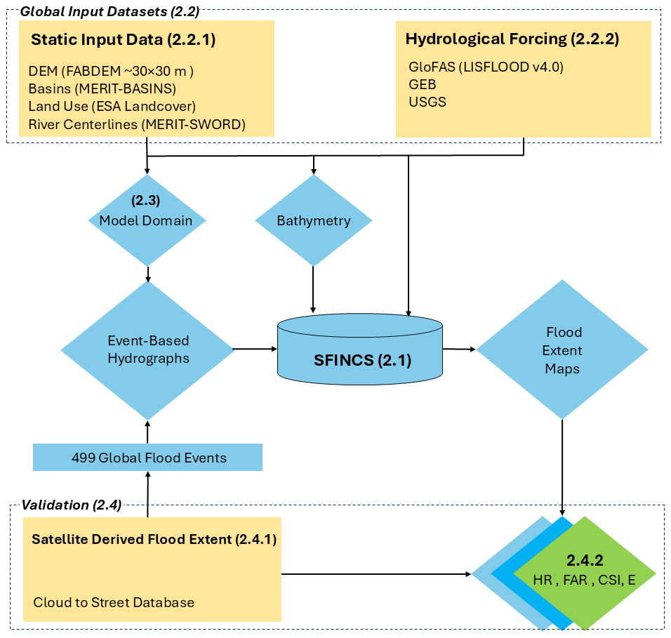
Figure 1 Automated framework for testing of the global hydrodynamic model SFINCS (section numbers are in brackets).

2.1 The hydrodynamic model SFINCS

SFINCS is a fully automated, 2D reduced-complexity hydrodynamic model that solves simplified Saint-Venant equations of mass and momentum (Leijnse et al., 2021). The model uses a localised inertial equation (LIE) formulation, which neglects advection, Coriolis force, and viscous effects, simplifying the full Saint-Venant equations (Bates et al., 2010). These simplifications significantly reduce computational costs while retaining sufficient floodplain accuracy (Leijnse et al., 2021). A comparison with full-physics models such as Delft3D (Deltares, 2022) revealed that SFINCS can achieve up to 100 times faster computation speed for equivalent domains with negligible loss in accuracy for sub-critical flow conditions (Leijnse et al., 2021). The model's reduced complexity enables rapid simulations, which makes it suitable for large-scale or global modelling applications like this study. For this study, we utilised SFINCS in subgrid mode to leverage its ability to integrate high-resolution elevation data while simulating flood dynamics efficiently across large river basins. We developed uncalibrated models by automating the model setup and execution process to ensure consistency and minimise manual intervention. While SFINCS was originally developed for coastal flooding applications, it has been adapted to model riverine flood events in this study. The fluvial setup focuses on river discharge as the primary forcing and incorporates several key additions to the coastal-oriented model configuration. These additions to enable fluvial flooding were as follows:

2.1.1 Bankfull width and depth estimation

These parameters determined the channel capacity of the rivers and thus indicate the moment after which inundation processes started. Calculating the bankfull discharge is explained in Sect. 2.2.3 and Appendix A1.

2.1.2 Hydrograph input and global model setup

We chose an automated event-based approach to assess the model's robustness and performance under varying conditions. Our simulations were structured event by event and assumed each observed flood event as a distinct and independent occurrence. The timings of the input hydrographs and model domain extent were derived from moderate resolution imaging spectroradiometer (MODIS) satellite observations, compiled into the Cloud to Street database (Sect. 2.4.1). This database includes a subset of 499 riverine flood events spanning five (sub)continents and 96 countries. To simulate floods on a global scale for each event, discharge data was obtained from global hydrological model LISFLOOD v4.0, as described in Sect. 2.2.2. Each event was processed and run separately, with all associated flooded basins (MERIT-BASINS) simulated in one model run. Notably, a single flood event can occur across multiple basins. We refer to these combined basins as the “model domain”. This setup allowed us to handle large-scale flood modelling tasks efficiently. By applying the model across many events, we validated the model across a wide range of flood magnitudes in different geographical (e.g. catchment sizes) and climatological settings.

2.1.3 Headwater and river inflow points

Discharge source points were set up in the SFINCS model to simulate water coming in from rivers. These source points can be river inflow points, which simulated water entering the model domain from upstream rivers (e.g. rivers that cross the boundary of the model). Water can also enter the model coming from headwater rivers, which are streams that originate inside the model domain. The start or origin of these headwater rivers is called the headwater point. Accurate placement of both headwater and inflow points is essential for reliable flood modelling since the misalignment of these points can lead to the significant over- or underestimation of downstream flooding, particularly during catchment-wide events where multiple tributaries converge into a main river channel. Therefore, to ensure hydrological consistency between the hydrodynamic model and the hydrological input (which is at a much coarser resolution), headwater and inflow points are snapped to the grid cell that best matches the upstream contributing area of the hydrological model used. This linkage between hydrological discharge and the hydrodynamic river network is based on upstream drainage area matching, a method commonly used in large-scale flood modelling frameworks (e.g. Eilander et al., 2023a). The use of a tolerance in upstream area ensures correct placement of forcing points, and the influence of hydrological input resolution on model performance is further evaluated in Sect. 2.5 Sensitivity Analysis.This snapping was implemented using the HydroMT-SFINCS plugin (see Sect. 2.3.1: Data handling and pre-processing). Discharge input for inflow and headwater points was sourced from multiple datasets, as described in Sect. 2.2.2. To account for differences in resolution and small mismatches in the upstream area, we applied a tolerance of 5 % deviation when snapping. This approach helped to ensure that discharge was applied at hydrologically consistent locations, which reduced the risk of errors in flood extent prediction due to poor spatial alignment between the hydrological and hydrodynamic models.

2.2 Global Input Datasets

2.2.1 Static Input Data

Static input data provided essential environmental and topographical information to the SFINCS model. The following datasets were used for the global automated setup which include:

Digital Elevation Model (DEM)

The FABDEM V1-2 dataset (Hawker et al., 2022) was used to provide elevation data at a global scale. This dataset has a 30 m resolution and is proven to be more accurate than existing global elevation datasets (Hawker et al., 2022).

Land-Use Data

Land-use patterns were derived from the ESA Worldcover 2021 dataset on a 10 m resolution (Zanaga et al., 2022). The land-use data was used to define Manning's roughness coefficient for different land-use types.

River Network Data

River geometries were obtained from the MERIT-SWORD dataset v0.4 (https://doi.org/10.5281/zenodo.14675925, Wade et al., 2025), which is a dataset created by combining the SWOT River Database (SWORD; Altenau et al., 2021) and MERIT-BASINS (Lin et al., 2019). The MERIT-SWORD dataset transfers data, such as river width from SWORD rivers (30 m wide and greater), to corresponding MERIT-BASINS rivers by generating bidirectional links. Drainage areas smaller than 25 km², including non-channelised areas along the coast or certain endorheic regions (e.g. incomplete basins or hillslopes), were excluded to maintain focus on larger river systems in this dataset.

Basin Delineation

The MERIT-BASINS dataset (Lin et al., 2019) was used to define the boundaries of individual basins. Each individual basin in MERIT-BASINS carried a unique basin identifier and an upstream area attribute that directly corresponded to a specific river reach in the MERIT-SWORD network.

2.2.2 Hydrological Forcing

Discharge data required to force the SFINCS model at predefined discharge points (headwater and inflow points) was obtained from three sources, two hydrological models and a database with observed discharges. The primary global dataset was GloFAS (Grimaldi et al., 2022), which provided long-term global coverage discharge data suitable for simulating floods at a global scale. The second source was the GEB model (De Bruijn et al., 2023), which generates higher-resolution behaviourally informed discharge estimates that are particularly useful in basins where human interventions significantly influence flood dynamics. Finally, observed discharge records from the USGS database (USGS, 2023) were used as a benchmark to evaluate the performance of the model predictions in selected US basins.

GloFAS (LISFLOOD v4.0)

The GloFAS dataset (Alfieri et al., 2013; Grimaldi et al., 2022) is generated using the global hydrological model LISFLOOD-OS, which is a distributed, physically based rainfall-runoff model that uses the ERA5 reanalysis data as input to simulate global river discharge at ∼5.5 km resolution at the equator. GloFAS discharge is primarily designed for river basins larger than ∼500 km² (Grimaldi et al., 2022). In this study, it is applied across a wider range of basin sizes to assess how model performance varies with basin scale when using globally available discharge datasets, including smaller basins. This allows us to evaluate the behaviour of the modelling framework under conditions where the input data may be less reliable. Because the timing of the peak discharges in GloFAS hydrographs can differ from the timing of the floods observed in the satellite-derived extent maps (Sect. 2.4), we captured GloFAS data 10 d before and 10 d after the timing of the flood event in the observed data. In this way, we are sure the flood event (i.e. discharge peak) was in the GloFAS dataset. The GloFAS dataset was used as the default dataset for discharge in the global automated setup. The GloFAS dataset was selected because it offers long-term, global coverage of discharge data, which made it suitable for simulating floods on a large scale. The following mentioned datasets were used in the sensitivity analysis for this study (Sect. 2.5):

GEB Model

The GEB model (De Bruijn et al., 2023) integrates an agent-based model (ABM) and a hydrological model to simulate the flood and drought management decisions of farmers and urban households interacting with the hydrological system. Within GEB, the ABM is dynamically linked with the spatially distributed grid-based hydrological model CWatM at ∼1 km resolution at the equator (Burek et al., 2020). The GEB model incorporates not only surface and groundwater hydrological processes but also the impacts of human activities like water consumption and reservoir operations. We used the daily discharge estimates from the GEB model as input to SFINCS during the sensitivity analysis (Sect. 2.5). The GEB model was selected because it captures socio-hydrological interactions and provides high-resolution, behaviourally informed discharge estimates, which are particularly useful in basins where human interventions significantly influence flood dynamics, such as the Krishna Basin in India, where it was applied in this study (see Sect. 2.5).

USGS Discharge Observations

The USGS (2023) provides real-time streamflow data, which we used as a benchmark to evaluate how well the global hydrological model's predicted discharge aligned with actual observations in a selection of US basins (Sect. 2.5). We limited the benchmark to US basins due to the availability of high-quality, long-term, and consistent discharge records from the USGS, which have been globally recognised for their reliability.

2.2.3 Bathymetry

Bankfull discharge represents the level at which a river fills its channel without overflowing and is a key threshold in determining the channel dimensions of a river. We followed the approach outlined by Sampson et al. (2015), using bankfull discharge as the primary indicator for estimating the river's cross-sectional shape. To calculate the bankfull discharge, we used the 2-year return period calculated from the GloFAS hydrological model discharge (Sect. 2.2.2). The 2-year return period was selected because it closely corresponds to the bankfull flow for many rivers, representing a typical flow regime that occurs frequently enough to shape the channel's morphology over time (e.g. Edwards et al., 2019). However, recent studies have shown that this threshold can vary significantly across different (sub)basins (Roy and Sinha, 2016). Therefore, we included a sensitivity analysis to assess the impact of this assumption (Sect. 2.5). This allows for modelling of channel dimensions based on recurrent hydrological conditions. We then assumed a rectangular cross-sectional shape for the river channels, which was burned into the DEM (for more detailed information, see Appendix A1).

To estimate the bankfull width, we primarily used values from the MERIT-SWORD database, which integrates observations from multiple global rivers and satellite-related datasets (see Sect. 2.2.1). For the river sections whose values were not represented in MERIT-SWORD, we applied a power-law relationship between bankfull discharge and channel width, as proposed by Leopold and Maddock (1953). This empirical relationship reflects how larger discharges are accommodated by wider channels, while smaller discharges are carried by narrower channels. This approach ensured consistency in width estimation where observational data was lacking and serves as a gap-filling strategy to ensure complete channel representation across the river network.

The bankfull depth was then calculated using Manning's open channel flow equation. This equation accounts for both riverbed roughness and slope. Importantly, the equation also incorporates the bankfull width either observed (e.g. from MERIT-SWORD) or estimated using the power-law relationship ensuring that depth estimates were consistent with the defined channel geometry.

In the sensitivity analysis, we also use the GEB model outputs and the USGS discharge time series to estimate the 2-year return period and the related bathymetry (Sect. 2.5).

2.3 Determining the Model Domains

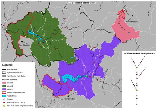
Basin delineation was guided by observed flood events, which are identified from satellite-derived flood maps (Cloud to Street database; Sect. 2.4.1). These events helped determine which basins were affected and how they were grouped together (here referred as “basin clusters”, see Fig. 2) during each flood. The following criteria were applied during this step to delineate the basins:

• Delineating basin clusters. We delineated clusters of hydrologically connected basins for each event to capture the structure and connectivity of flooded areas within a catchment. First, we identified which HydroBASINS Level 8 basins were flooded. Flooded basins touching the coastal areas were excluded from the analysis; only inland basins were considered. Then, we used these flooded HydroBASINS as a guide to select MERIT-BASINS, which ensured the simulation areas were neither too large nor too small. As a result, the model domain regions were not larger than HydroBASINS Level 8, which kept the SFINCS simulations efficient. Next, we focused on converting the MERIT river network into a directed graph based on downstream flow connectivity (Fig. 2B). Using the river network graph, we built a network of basins that were hydrologically connected. Next, we identified flooded basins by overlaying the observed flooded pixels from satellite imagery with MERIT-BASINS boundaries. Any basin that intersected with observed flood pixels (based on the aforementioned criteria) was marked as flooded. We also included a user-defined number of downstream basins (default: 1 basin) into the simulated area. Doing so helps to reduce the “boundary effects” problem that could happen at the edges of the simulation when water could not flow properly out of the model area. Including downstream areas aimed to help prevent distortions near the outflow edge and maintain flood flow dynamics in the hydrodynamic simulations. Subsequently, we analysed the resulting set of basins (flooded MERIT-BASINS + 1 downstream basin) and group them together in a cluster, as illustrated by the subsets shown in Fig. 2 (e.g. Subsets 1–3). Each cluster represented a distinct set of hydrologically linked basins affected by the same flood event. Subsequently, we ran the hydrodynamic simulations (SFINCS) for each cluster separately using snapped (see Sect. 2.1) discharge points with simulated discharge as input into the model domain. This approach ensured that the full spatial structure of each flood event was respected, enabling more realistic hydrodynamic modelling across complex river networks.

• Flooded pixel area (>1 % model domain area). The flooded pixel area after the delineation should cover more than 1 % of the basin cluster area. This approach ensured that basins without a substantial flood were excluded to omit irrelevant model runs and shorten run times.

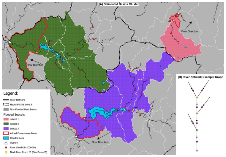
Figure 2 (A) An example of a delineated basin cluster for flood event observed between 22 December 2013 and 4 January 2014 in the United States, showing how individual basins affected by the flood were grouped based on hydrological connectivity. (B) An example river network graph used to represent downstream flow connectivity between basins, as derived from the MERIT river network.

2.3.1 Data handling and preprocessing

We used the HydroMT package (Eilander et al., 2023a) to set up a separate model for each basin cluster across all events. HydroMT handled the automatic data processing and configuration of the SFINCS hydrodynamic model while integrating multiple data sources (e.g. hydrographs, DEMs, and land-use maps). This automation reduced potential errors in manual data processing and enabled the rapid testing of different scenarios. The modular setup of the model allows for further iterative enhancements to the model, ensuring it can effectively adapt and improve as new data is integrated over time. To run both HydroMT and SFINCS for all clusters and events, we further automated our approach using Snakemake (Mölder et al., 2020), a Python-based workflow management system to manage parallel simulations efficiently. Appendix Sect. A2 explains the use of Snakemake and the data handling of our study in more detail.

2.4 Validation

2.4.1 Satellite-Derived Flood Extent

A validation procedure was designed to validate the simulated flood extents predicted by the SFINCS model. We evaluated whether these simulated flood extents aligned with satellite-derived flood events provided by the Cloud to Street (2022), also known as the Global Flood Database. This database was selected because it offered several key advantages for this type of analysis. Firstly, the database provided global coverage, which ensured that flood events from diverse regions around the world were represented. Secondly, it organised all satellitederived flood events into clear categories of flood drivers. Thirdly, the data was openly accessible and downloadable, which streamlines integration into research studies. Importantly, all the flood maps were consolidated under a single dataset, which eliminated the need to combine multiple data sources.

The database was developed using data from NASA's MODIS satellite which captures daily flood extents documented by the Dartmouth Flood Observatory (DFO) with a spatial resolution of 250 m. MODIS provides consistent global coverage with a daily revisit cycle, making it well-suited for large-scale flood monitoring. The full dataset included 913 observed flood events from 2000 to 2018 (Tellman et al., 2021), which represented the maximum observed surface water extent over the event duration. However, it is important to note that these maximum flood extents may be underestimated due to limitations such as cloud cover, vegetation, or narrow channels that may obscure floodwaters in the satellite imagery (Tellman et al., 2021). To prepare the dataset for validation, we selected events (n=499) from the full database by applying the following filters:

• Flood type in observations (heavy rain only). The global flood database lists the main flood drivers, which we filtered only to include floods caused by “Heavy Rain”, which excluded other flood drivers such as tropical storm surge, dam breaks.

• Flood duration (<30 d). Floods lasting more than 30 d were excluded because the satellite-observed flood images in the analysis are composite images created from multiple days of observations. During longer flood events, the flood extent may change over time, potentially leading to inaccurate or mixed representations of the flood. By focusing on shorter floods, we ensured that the composite images more accurately reflected the flood's maximum extent, avoiding the temporal variations that can occur during longer-lasting floods. This approach improved the reliability of the flood extent data used for model validation and analysis (Cloud to Street, 2022).

• Permanent water-body masking. Permanent water bodies were masked from the observed flood dataset by removing permanent water pixels extracted from the JRC Global Surface Water Mapping Layer v1.1 (Pekel et al., 2016). This procedure excluded pixels that were always flooded (e.g. the rivers themselves and large parts of reservoirs) to ensure that only genuinely flooded areas which are not typically inundated were included in the analysis. These permanent water features are always present and do not reflect new inundation caused by flooding events. This helped in accurately assessing flood extents and refining the validation of hydrodynamic models based on observed flood extent (Fleischmann et al., 2019).

2.4.2 Validation Metrics

We computed the maximum flood extent across all time steps to generate a single inundation map representing the peak of the event for every SFINCS simulation. The observation data only showed if a pixel was flooded or dry (without depth data), so we also changed the SFINCS output to a pixel with only two states: either flooded or dry. In a postprocessing procedure, a minimum depth of 0.05 m was used to classify a pixel as flooded (Wing et al., 2024). Note that we resampled the high-resolution SFINCS outputs of 30 to 250 m using mode resampling to match the resolution of observed flood extents. This approach avoids downscaling the MODIS observations, which would require disaggregation of coarse resolution pixels and could create observed flooded pixels outside the actual flooded areas. By aggregating the model outputs to the resolution of the observations using mode resampling, a consistent comparison between simulated and observed flood extents is ensured. This approach meant that a 250 m SFINCS output pixel was classified as flooded if the majority (i.e. more than one-half) of the underlying SFINCS 30 m cells were flooded. This method ensured consistency with the binary “flooded or dry” classification of MODIS data while reflecting the majority condition in each area. Notably, the permanent water bodies (already 250 m), identified from band 5 of the satellite data, were also masked from the SFINCS simulated flood event after it has been resampled to 250 m. Importantly, the additional downstream basin included in the model domain to avoid boundary effects was not considered when applying the validation criteria. This approach ensured that the validation only assessed the basins directly affected by flooding to provide a fair comparison between the simulated and observed flood extents.

Table 1 shows the validation metrics used to compare SFINCS results with the observations. We validated our maps for each flood event by calculating the contingency table values (i.e. Hit, Miss, False Alarm, and Correct Negative) over the full extent (i.e. all basins) of the event.

Table 1 Contingency table used to calculate the SFINCS validation metrics.

Hit Rate (HR; Eq. 1)

The HR measures the proportion of the flood area observed that was successfully predicted by the model, balancing misses (Miss) and hits (Hit). The HR can range from 0 to 1. A higher HR indicates better model accuracy in terms of correctly predicting the flood extent.

$$\begin{array}{}\text{(1)}& \text{Hit Rate}={\displaystyle \frac{\text{Hits}}{(\text{Hits}+\text{Misses})}}\end{array}$$

False Alarm Ratio (FAR; Eq. 2)

The FAR represents the proportion of predicted flood areas that did not flood in satellite-derived flood extents. The FAR can range from 0 to 1. A low FAR suggests that the model is conservative in its flood predictions.

$$\begin{array}{}\text{(2)}& \text{FAR}={\displaystyle \frac{\text{FA}}{(\text{FA}+\text{Hits})}}\end{array}$$

Critical Success Index (CSI; Eq. 3)

The CSI balances the HR and FAR in Eqs. (1) and (2) to provide a comprehensive metric of the overall model performance. The CSI can range from 0 to 1, with 1 indicating a perfect model. The CSI accounts for correct predictions (i.e. Hits) and wrong predictions (i.e. Misses and FAs), offering a more nuanced view of model accuracy.

$$\begin{array}{}\text{(3)}& \text{CSI}={\displaystyle \frac{\text{Hits}}{(\text{Hits}+\text{FA}+\text{Misses})}}\end{array}$$

Error Bias (E; Eq. 4)

E is a metric used to determine whether a model is overpredicting or underpredicting the occurrence of an event, such as flooding. A value of E=1 indicates no bias, meaning the model's predictions are balanced between overprediction and underprediction. If E falls between 0 and 1, the model tends to underpredict, while values greater than 1 suggest the model overpredicts the event.

$$\begin{array}{}\text{(4)}& E={\displaystyle \frac{\text{FA}}{\text{Misses}}}\end{array}$$

2.5 Sensitivity Analysis

The sensitivity analysis focused on how variations in key parameters affected the SFINCS model's flood predictions. For this study, we focused on three critical factors: river depth estimation, elevation data, and discharge data. These parameters were chosen because they directly influenced flood extent predictions, and variations in their accuracy can have significant implications for model performance in large-scale flood modelling. The rectangular cross-section used in SFINCS is a widely adopted representation in hydrodynamic modelling (e.g. Neal et al., 2012). Floodplain roughness values were spatially varied based on land use data (ESA Land Cover), while a constant Manning's roughness value (n=0.02) was applied for river channels to ensure consistency across the large number of basins and regions considered. This constant value has been used by other studies (Bril et al., 2026) and similar approaches using fixed channel roughness values are commonly adopted in large-scale flood modelling studies (e.g. Yamazaki et al., 2011; Dottori et al., 2016; Neal et al., 2012). For the sensitivity analysis, we focused on two geographical regions: the US and India. We selected the flood events from the Global Flood Database using the DFO's “Severity Level 2” classification (Tellman et al., 2021), which identifies floods with high impacts (recurrence interval >100 years). The severity level was a criterion for choosing representative events for the sensitivity analysis. This selection identified ten US events and 11 events in India for our sensitivity runs.

2.5.1 River depth estimation

To test the effect of our bathymetry estimation method, we used different return periods (1.5-year, 2-year (default in global setup) and 2.5-year) following Andreadis et al. (2013) to estimate bankfull discharge (see Appendix A1) and assess their impact on flood dynamics. We used GloFAS discharge to estimate bankfull discharge for rivers by applying different return periods. For some rivers, bankfull discharge might correspond to a higher or lower return period, so using the same return period for all rivers might not give accurate estimates of river bathymetry and flood extents (Roy and Sinha, 2016; Rad et al., 2024). Therefore, testing multiple return periods provided a better understanding of the river's bathymetry.

2.5.2 Elevation data

Different DEM resolutions (FABDEM 30 m vs. 3D Elevation Product 3DEP 1 m) were compared to assess the impact of topographic resolution on flood modelling. Higher-resolution DEMs often provide more accurate flood predictions, particularly in areas with complex terrain (Jiang et al., 2022).

2.5.3 Discharge data

The model's sensitivity to discharge inputs was tested by forcing the model with USGS observation discharge instead of simulated discharge from GloFAS. Thus, the actual event forcing and river channel size estimates were updated based on the observed discharge. Accurate river discharge input is crucial for hydrodynamic modelling, as it directly influences flood predictions (Zhou et al., 2022). This comparison between modelled (GloFAS, default input) and observed (USGS) discharge allowed for disentangling the source of the modelling errors from either the inflow or the processes within SFINCS. USGS River discharge data were filtered for locations containing data for more than 30 years to ensure that return periods and thus bathymetry was more accurately predicted.

Furthermore, to ensure robustness and avoid reliance on a single hydrological model, we also forced SFINCS with the GEB model discharge (Sect. 2.2.2). However, GEB is currently not available as a global dataset and is still under development for large-scale applications. As a result, its use in this study was limited to a subset of case studies rather than the full global event set. This comparison was designed to test the sensitivity of SFINCS to hydrological input characteristics since GloFAS and the GEB model fundamentally differed in model resolution. The GEB model discharges were specifically tested in the Krishna Basin in India (11 riverine events), a large and significant river basin known for its significance due to its size being nearly 8 % of the total geographical area of India and extensive agricultural and hydrological use. The GEB discharge outputs were used to drive the flood simulations and derive river channel dimensions. The resulting inundation extents were compared against the Cloud to Street database to assess model accuracy. This dual-model comparison between GloFAS and GEB provided insights into variability and reliability across different hydrological sources with different resolutions, thereby strengthening the analysis of SFINCS flood simulations.

3 Results and Discussion

Here, we present the outcomes of the validation by first describing the general results at the global and continental scales (Sect. 3.1). To better understand spatial differences in model performance, we also focus specifically on the continental United States (Sect. 3.4). Next, we explore how sensitive our results are to three key inputs: hydrological forcing, bathymetry, and DEM (Sect. 3.6). Finally, we compare our findings with other similar studies, discuss the model's limitations, and identify areas for future improvement (Sect. 3.7).

3.1 Global Performance Results

We set up the SFINCS model for 499 riverine flood events worldwide in our validation dataset (Sect. 2.4.1). These simulations were created using discharge from the global hydrological model GloFAS and validated against satellite-derived flood extents. To calculate the global performance metrics shown in Table 1, we aggregated the results across all simulated events by summing the total number of pixels in each classification category (i.e. Hit, Miss, and FAs) across all events (Sect. 2.4.2). This analysis gave more weight to larger flood events (with more pixels) by summing all pixels across all events, which avoided biasing the results by treating small and large events equally when calculating the mean.

Table 2 shows that the model achieved an HR of 0.58 for simulated discharge, meaning that 58 % of the observed flooded pixels were correctly simulated. The CSI, which balances both Misses and FAs, had a global mean value of 0.39. E was 1.24, which indicated an overestimation of flood extent across events.

Table 2 Event-based performance metrics over 499 events all over the globe, as calculated by comparing SFINCS simulations to the satellite derived flood extents.

3.2 Effect of Upstream Basin Area on Performance

Table 3 shows considerable variety in the performance metrics across basins with different upstream area sizes. We classified basins into five different upstream area size classes and compared them using the same model runs, hydrological inputs, and observational data as in the above-described global analysis. Most flood events that we simulated in this exercise involved multiple MERIT-BASINS (i.e. sub-basins) that were hydrologically connected. For this analysis, we split the simulated flood event into individual MERIT-BASINS and assigned an upstream area to each basin by determining the contributing drainage area at the subbasin outlet, as defined by Lin et al. (2019). Notably, the total number of basins varied significantly across the upstream area classes. We note that GloFAS discharge is generally recommended for basins larger than approximately 500 km² (Grimaldi et al., 2022; Baugh et al., 2024). In our dataset, approximately 61 % of the analyzed basins fall below this threshold (n=16 225), while 39 % are ≥500 km² (n=10 367). This allows us to explicitly assess how model performance changes across basin sizes, including those where the hydrological forcing is expected to be less reliable. Basins with a large upstream area (≥1000 km²) were the most represented group (n=8834) as compared to basins with a medium-sized upstream area (500 to 1000 km²; n=1533).

Table 3 Performance of the SFINCS flood simulations, classified by basin upstream area (Clipped from the same model runs).

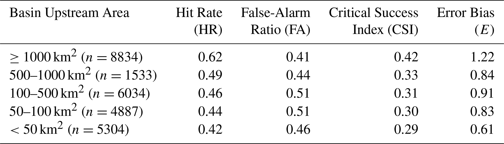
The analysis showed a clear trend of increasing model performance with increasing upstream basin area. Specifically, the average CSI rose from 0.29 in the basins with a small upstream area (<50 km²) to 0.42 in the basins with a large upstream area (≥1000 km²). This result aligned with prior studies that have either excluded basins with a small upstream area altogether or reported lower accuracy for them (e.g. Wing et al., 2017; Bernhofen et al., 2018). Three main reasons exist for this scale-dependent behaviour.

1. Firstly, smaller upstream basins often suffer from poorly defined or incomplete river networks (Fig. 3a) that result in missing discharge forcing at these locations and can introduce substantial structural errors in the flood extent simulations. For instance, global hydrography datasets like MERIT-SWORD used in this study typically include only river channels with drainage areas larger than 25 km². As a result, key hydrological pathways may be missing or truncated in basins with very small upstream areas, which leads to a significant underestimation of the inundated area. However, even upstream areas exceeding this 25 km² threshold can still contain errors or missing tributaries, which affect the accuracy of the simulated flood extents. This limitation is illustrated in Fig. 3a, where a small upstream catchment shows a river stretch with an upstream area of 40.5 km². However, a smaller contributing river upstream is absent from the dataset, which resulted in missed flooding (red pixels) despite clear observational evidence.

2. Secondly, larger upstream basins benefit from the spatial averaging of hydrological processes. As seen in Fig. 3b and c, mid-sized to large-sized upstream basins integrate runoff contributions from diverse upstream areas and multiple tributaries, which dampens localised anomalies and smooths the overall hydrological signal (Bernhofen et al., 2018; Salinas et al., 2013). These outcomes lead to more predictable and consistent flood responses, especially in models forced by coarsely resolved (∼5.5 km resolution) inputs like GloFAS (Harrigan et al., 2020).

3. Thirdly, hydrological forcing becomes more uncertain in small basins, where local rainfall-runoff processes dominate and are poorly captured by global-scale models (Smith et al., 2014). Coarse meteorological input data and simplified rainfall-runoff representations are less effective at resolving the fine-scale variability that drives flooding in these areas (Harrigan et al., 2020). Consequently, smaller upstream basins tend to show lower HRs compared to larger ones. Table 3 supports this interpretation. The model performed best in large basins (≥1000 km²), where it achieved the highest HR (0.62) and lowest FAR (0.41). In contrast, basins under 50 km² showed an HR of 0.42, a FAR of 0.46, and a CSI of just 0.29. Interestingly, these smallest basins also exhibited the lowest error bias (E=0.61), which suggests that underprediction was more common than overprediction. This underprediction can potentially be reduced by also including a pluvial setup which accounts for direct rainfall-driven flooding within these smaller basins.

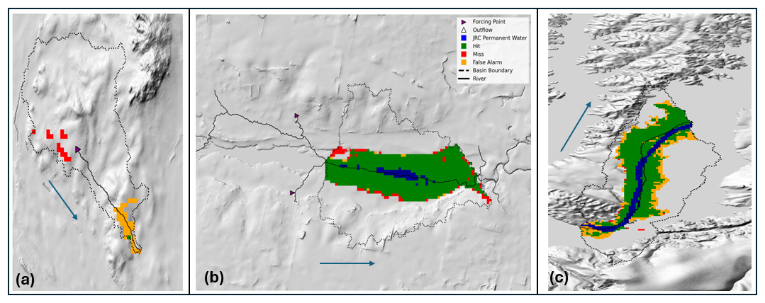
Figure 3 Some example flood events illustrating that with increasing basin sizes, the number of hits increases as well: (a) small upstream basin (40.5 km²) with a river channel (black) that does not connect to a potential flood zone in the north, which results in misses (red area); (b) mid-sized basin 500–1000 km²; (c) large-sized basin of >1000 km². Flow direction is shown with a blue arrow.

These results highlight the effect of upstream basin area in global flood modelling and the need to better understand the processes in small upstream catchments in large-scale studies. Analysing them separately rather than excluding them, as done in some previous efforts (e.g. Wing et al., 2017), can offer valuable insights into improving model performance in these challenging regions.

3.3 Model Performance in Different Climate Zones

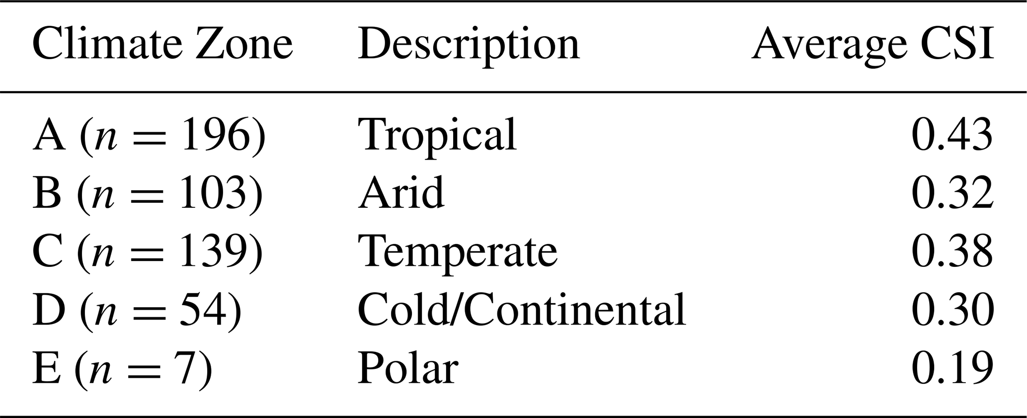
To investigate the influence of climatic variations on model performance, each basin simulation was classified according to the Köppen-Geiger climate classification (Beck et al., 2018) using the centroid of each basin. Individual climate subclasses were grouped into the main climate classes: A (Tropical), B (Arid), C (Temperate), D (Cold/Continental), and E (Polar). This analysis was conducted for individual basins instead of flood events because flood events can occur over very large spatial scales and across multiple climate zones. Thereby, individual basins are weighted equally, meaning that smaller basins contribute to the overall average CSI in the same way as larger basins. The results show clear variation in model performance across climate zones (Table 4). Performance is generally higher in tropical and temperate climates, where CSI values are 0.43 and 0.38, respectively. Lower performance is observed in arid climates with an average CSI of 0.32, while cold/continental climates show further reduced performance with an average CSI of 0.30. The lowest performance is observed in polar climates with an average CSI of 0.19. It is worth mentioning that most of the events simulated are based in Tropical (n=196) and Temperate (n=139) climate zones.

Table 4 Model performance grouped per main climate zone. The number of flood events per zone is shown in brackets.

This pattern is consistent with known limitations of both global hydrological models and satellite-derived flood observations in cold and polar regions, where snow and ice dynamics, frozen soils, and limited river gauges reduce the reliability of both the forcing data (GloFAS discharge; Harrigan et al., 2020) and the flood observations (Tellman et al., 2021). Performance of large-scale hydrological models in arid regions is usually lower compared to temperate and tropical regions (Salinas et al., 2013), as flooding in arid regions is driven by short intense rainfalls that are difficult to capture by hydrological models (Smith et al., 2014; Harrigan et al., 2020). In addition, runoff generation is highly variable due to infiltration and transmission losses in arid and semi-arid river channels, making peak flows harder to estimate (Dottori et al., 2016). Overall, these results suggest that the modelling framework performs most reliably in tropical and temperate climates, and that performance in arid and cold/polar regions is much lower

3.4 Model Performance Across Continental US Basins

Figure 4 shows the spatial distribution of CSI values across all basins within the US, where 52 flood events recorded in the Cloud to Street database were analysed. Note that in Fig. 4, each MERIT-BASIN was validated individually, as explained in Sect. 3.2. When calculating the mean CSI over the continental US, we considered all pixels of the 52 events modelled using GloFAS discharge. The results showed that the average model performance was slightly higher in the US (CSI=0.41, including the small basins <50 km²) as compared to the global average (CSI=0.39). The colour gradient signifies the range of CSI values, with red representing lower scores (CSI≤0.2), orange representing the mid-range ($\mathrm{0.2}\le \text{CSI}\le \mathrm{0.4}$), and light green ($\mathrm{0.4}\le \text{CSI}\le \mathrm{0.6}$) and dark green indicating higher scores (CSI≥0.6). Distinct spatial patterns emerged with clusters of bad-performing basins (CSI≤0.2) in two parts of the US (Fig. 4a and b).

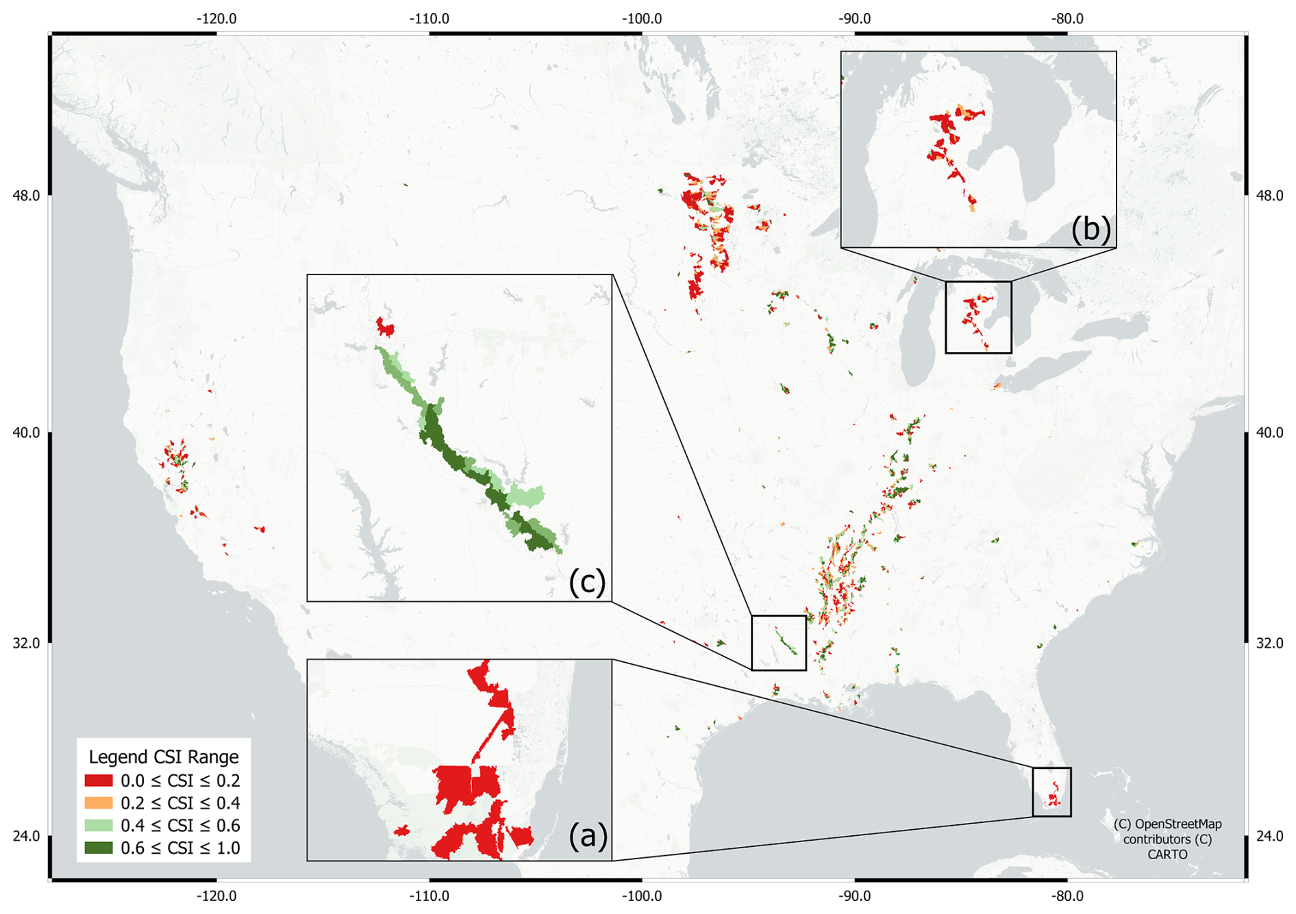
Figure 4 Spatial map with CSI performance numbers for the US. The red colours indicate clusters of low-performing basins; the light and dark green colours represent better-performing basins. The panels zoom in to the following regions: (a) Florida, (b) the Great Lakes, and (c) Mississippi. Base map © OpenStreetMap contributors, rendered with Carto, licensed under ODbL.

Firstly, we see that in Fig. 4a the region of Florida performed consistently low, with many individual basins showing CSI values below 0.2. Florida is a low-lying, flat region, which makes flood simulations particularly challenging (Hawker et al., 2022). Furthermore, we observed that all 45 individual MERIT-BASINS with poor performance corresponded to a single flood event (i.e. DFO_3544), which yielded an average CSI of 0.28 across the affected basins. Potential uncertainty also existed in the DFO_3544 flood type validation (notably, dfo_validation_type = 0, which indicated this event's primary confirmation source as undefined or missing). This means that the event, while classified under “Heavy Rain,” could also have been influenced by other flood drivers. The low scores partly resulted from both regional and event-specific limitations, such as DEM errors or challenges in detecting floods with optical remote sensing in flat, low-relief terrain (Tellman et al., 2021).

Secondly, model performance was also generally poor in the Northern Continental US near the Great Lakes (Fig. 4b), with multiple basins exhibiting CSI values below 0.3. Notably, only two events (i.e. DFO_2606 and DFO_2412) contributed to the majority of low CSI values in this region. For the dominant event in this region (i.e. DFO_2606), the HR was 0.73, while E=1.36 and FAR=0.62 indicated that the low CSI values were driven primarily by overprediction of the flood extent. Further investigation into DFO_2606 revealed that it corresponded to a severe winter storm that affected the Northeastern US between 5 and 6 January 2005. According to the National Weather Service (2005a), the storm brought heavy snow and freezing rain, followed by power outages and ice damage. Subsequent river flooding was reported in the vicinity of the Great Lakes. However, MODIS satellite data used in the Cloud to Street dataset only captured a brief cloud-free window on 9 January 2005, several days after the event's peak. The MODIS imagery, published by NASA (National Weather Service, 2005b), shows swollen rivers like the Ohio, Wabash, and White rivers. However, flooding is difficult to detect in snow-affected, cloudy, or densely vegetated areas (Tellman et al., 2021). Moreover, since MODIS flood extents reflect surface water conditions only during cloud-free acquisitions, the full flood footprint could have been underestimated or misaligned with actual peak inundation.

The third cluster represented good performance (Fig. 4c), near the Mississippi River. These basins had an average CSI of 0.43. Notably, the cluster was largely associated with a single event (i.e. DFO_4337), which could suggest this event had good agreement between the observations and simulations. Many of these basins also had large upstream contributing areas, which, as discussed in Sect. 3.2, tend to improve simulation accuracy due to more defined river networks and better-integrated hydrological processes stemming from the hydrological model.

3.5 Other Factors Influencing Performance

We identified several other factors that considerably affected model performance related to (1) resampling, (2) snapping and channel width in headwater catchments, (3) observed water bodies, and (4) coarse resolution and inflow points.

3.5.1 Resampling

Figure 5a shows that in regions with a good agreement between the SFINCS simulation and the satellite observations (Event DFO_4075; CSI=0.55), the resampling of a higher-resolution SFINCS output (30 m) to match the observations (250 m) introduced rough edges where the simulation could not match the boundaries of the observed inundation extent. These rough edges produced misses (red areas in Fig. 5a) around the boundaries, even when the true flood extent lay just inside the 250 m cell.

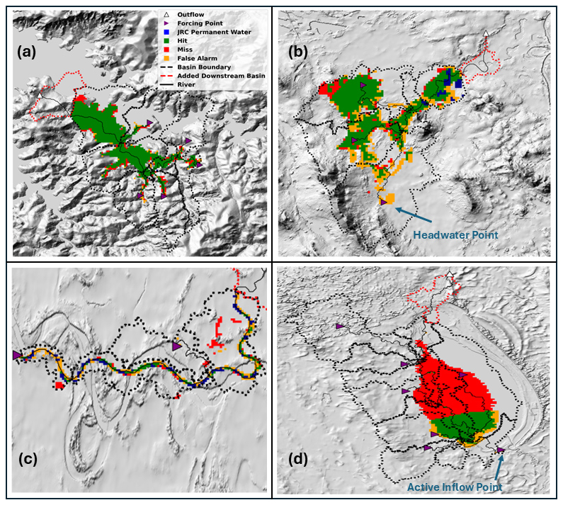
Figure 5 Model simulations across diverse regions illustrating the effect of (a) resampling with some misses on the rough edges of the simulated flood, (b) snapping and channel width, (c) missing observed water bodies, and (d) the influence of coarse resolution of discharge data on missing discharge into inflow points (Appendix A, Fig. A1).

3.5.2 Snapping and channel width in headwater catchments

Figure 5b (Event DFO_1996; CSI=0.48) showed inconsistencies (i.e. FAs) occurring in the headwater rivers. These inconsistencies could have arisen from several factors, such as the snapping procedure (Sect. 2.1.3). For example, in headwater locations, the coarse GloFAS grid (∼5 km) often misaligned with the finer SFINCS grid, so even with a 5 %–10 % snapping tolerance (see Sect. 2.1), small discharge mismatches were introduced into headwater tributaries, which in these narrow channels could produce localised FAs (yellow pixels in Fig. 5b) in areas that did not flood. Furthermore, we did not have width observations, so headwater river widths were estimated from the power-law equation (Sect. 2.2.3). This approach can sometimes under- or overestimate channel widths in smaller headwater rivers. If the equation gives too-narrow widths, conveyance capacity is underrepresented, which forces excess water onto adjacent floodplains (causing false alarms) (Dey et al., 2022). Conversely, if the equation gives too-wide widths, the simulated flood may be unrealistically confined to the channel and lead to misses.

3.5.3 Observed water bodies

Figure 5c depicts a region (Event DFO_4140; CSI=0.178) where permanent water was not well represented in the underlying observation layer of the Cloud to Street dataset (i.e. band 5). Although both the model and the satellite-derived flood extent relied on the JRC Global Surface Water dataset as a permanent water mask, the Cloud to Street product provided a 250 m resampled version (Tellman et al., 2021). When rivers meander or curve and are narrower than a MODIS pixel, the resampling process causes permanent open-water bodies to disappear. As a result, channels that are correctly simulated as inundated by SFINCS are not flagged as water in the observation layer and are instead counted as FAs during validation. This effect was particularly visible in low-order rivers where the channel was below 250 m wide. In these cases, the issue was not that the model overpredicted flooding but that the validation mask failed to represent permanent water bodies.

3.5.4 Coarse resolution and inflow points

In Fig. 5d, the region's (Event DFO_4451; CSI=0.177) lower performance was due to only one discharge point (i.e. inflow point) carrying water into the model domain. The other discharge points (i.e. headwater points) remained dry (see Appendix A, Fig. A1), which was likely caused by the coarse resolution (∼5.5 km²) of the GloFAS input discharge data. Thus, the model failed to capture peak flows in smaller upstream tributaries (Alfieri et al., 2013; Grimaldi et al., 2022), which created a significant gap in the simulated flood where the satellite observations clearly showed inundation.

3.6 Sensitivity Analysis

3.6.1 The influence of Hydrological Forcing

We conducted a two-part sensitivity analysis in two global regions (i.e. India and the US) to evaluate the role of hydrological forcing in our global flood modelling framework. We investigated (a) the differences in model performance when using two different global hydrological models (i.e. GloFAS and GEB) for 11 Events in India and (b) the influence of modelled GloFAS discharges compared to observed discharges for ten basins in the US.

(a) Comparing the influence of GloFAS discharge with GEB discharge

To compare the influence of using two different global hydrological models (GLOFAS and GEB) as input to SFINCS, we focused on the Krishna Basin in India. Here, we simulated floods for 11 discrete events with both models. Bathymetric calculations were done separately, using both GloFAS and GEB long-term discharges (>40 years) to compare all aspects of the two models. Using the GloFAS model discharge as forcing for SFINCS resulted in an average CSI of 0.34, while forcing with the GEB model led to an average CSI of 0.38.

One critical distinction between the two models lies in their spatial resolution. The GloFAS operates at a coarser grid resolution (∼5.5 km), while the GEB provides discharge data at a finer grid resolution (30^′′; ∼1 km). An example basin cluster within the Krishna basin is shown in Fig. 6 (Event 3551). The hydrographs on the right (Fig. 6) show the discharge forcings from both hydrological models at six main discharge points of the SFINCS simulation.

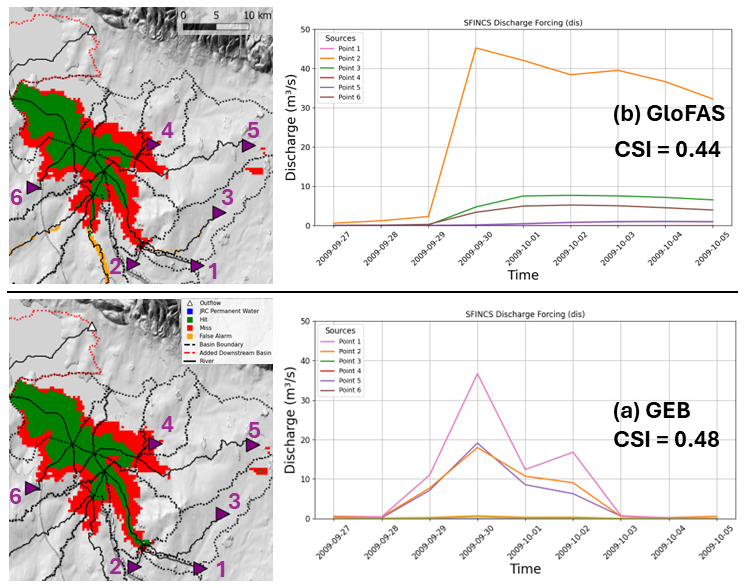
Figure 6 The sensitivity of SFINCS performance to different hydrological forcings by (a) the GEB model and (b) the GloFAS model is shown for a zoomed-in region in the Krishna Basin.

Notably, the GEB hydrographs exhibited a more complete flood hydrograph shape, especially toward the later stages of the event (Fig. 6). In contrast, the GloFAS hydrographs of some of the inflow points did not capture a high peak flow, suggesting that peak flows could be underrepresented. This issue directly affected the resulting flood maps (Fig. 6a and b, left panels), where simulations using the GEB input captured more hits than those driven by the GloFAS.

The improved performance of the GEB-SFINCS chain may be attributed to its higher spatial resolution, which allowed for a more accurate representation of smaller headwater rivers and their channel dimensions. In contrast, GloFAS lacks the ability to resolve these smaller streams directly, so bathymetric calculations relied on the nearest available grid point, which might not have aligned with the true upstream location. With the GEB, however, the finer resolution enabled matching bathymetry calculations to the correct upstream grid pixel, which resulted in more accurate low flows and a better representation of channel dimensions in smaller rivers. By resolving finer spatial scales, higher-resolution models like the GEB reduce uncertainties associated with inflow dynamics and provide more reliable input for hydrodynamic models like SFINCS. Moreover, the improved representation of human behaviour and reservoir management in the GEB can lead to more realistic streamflow estimates, which in turn enhances the accuracy of the flood simulations. This outcome underscores the importance of investing in higher-resolution global datasets to improve flood modelling accuracy in river systems.

(b) Comparing GloFAS discharge with observed discharge in the US

This section describes our assessment of the performance of our modelling setup by comparing modelled discharge from GloFAS with observed discharge data from the USGS (2023). The analysis evaluated model performance using event-based hydrographs from the GloFAS and USGS. Because this analysis could only be applied in regions with long-term discharge records (e.g. for bathymetry estimation), only ten distinct basin clusters remained suitable.

The results revealed that the model using observed USGS discharge data considerably outperformed the one using GloFAS discharge data by achieving an average CSI of 0.67 compared to the average global mean of 0.39 (Table 2). This significant difference shows the importance of accurate discharge data for enhancing model accuracy while highlighting the limitations of global hydrological models. Figure 7a and b provide insights into one such high-performing basin forced with USGS observations (CSI=0.78), while the same basin forced with GloFAS discharge yielded a lower CSI of 0.56. Nonetheless, a considerable number of misses occurred, even when observed discharge data were used. These misses can be explained by the resampling causing the rough edges. Furthermore, in the northeastern part of the basin (Fig. 7b), a side stream showed underprediction (i.e. misses), which was likely due to the absence of a river gauge in that tributary. Thus, to better represent this basin, an additional discharge input should be provided to reflect the flood extent accurately. A disadvantage of working with observational river gauges is the potential for gaps in spatial coverage, such as the side stream shown in Fig. 7b, which can limit model performance.

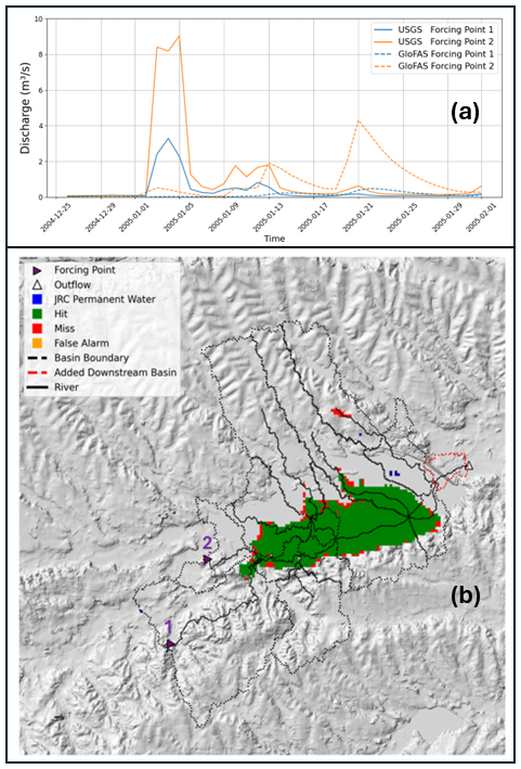
Figure 7 (a) Hydrograph analysis during the flood event. The dotted line represents the discharge from the GloFAS model, and the solid line represents the observations obtained from USGS. (b) Results from a high-performing US basin (CSI=0.78) forced with observed discharge input from the USGS. Forcing points 1 and 2 correspond to the hydrograph shown in panel (a).

Figure 7a shows the hydrograph during the flood event for both modelled (i.e. GloFAS) and observed (i.e. USGS) discharge data. The GloFAS hydrograph failed to capture the peak discharge during a flood event, which contributed to its lower performance (CSI=0.56) compared to the USGS-based forcing. The inability to capture discharge peaks decreased the precision of the simulated flood extents during high-flow conditions. Harrigan et al. (2020) showed that river discharge is negatively biased in 64 % of the basins globally in the GloFAS archive. Moreover, they reported that GloFAS-ERA5 discharge skill, measured by the Kling–Gupta efficiency (KGE), is strongly catchment-size-dependent: median KGE is only 0.21 for basins <10 000 km² (e.g. Fig. 7b basin has a catchment size of ∼500 km²), which rises to 0.56 for basins >50 000 km². This failure to capture discharge peaks in smaller basins has a more immediate and direct impact on flood extent simulations and can reduce the performance of the flood simulations.

3.6.2 Bathymetry

A fixed 2-year return period for bathymetric calculations is commonly used as a proxy for bankfull discharge, but this approach may not be universally applicable (Andreadis et al., 2013). Adjusting this parameter based on the characteristics of specific river systems could improve the accuracy of bathymetric estimates and better reflect actual flood behaviour (Roy and Sinha, 2016). Thus, this section presents our evaluation of how model performance was affected when different return periods were used to derive bankfull discharge in the SFINCS fluvial setup. We compared GloFAS-derived discharge with observed USGS river gauge data for ten US basins to assess the accuracy of bathymetry estimates.

The bankfull discharge was calculated via long-term yearly maxima peaks extracted from the GloFAS hydrological model and was evaluated against observed data from USGS river gauges. The results showed that the modelled bankfull discharge (Qbf) was consistently underestimated across all tested return periods.

Figure 8 shows the simulated Qbf (2-year RP) against USGS-derived Qbf on a logarithmic scale. All points lay below the 1:1 line, which indicated that the GloFAS-based RP were systematically lower, particularly in the lower quartile of values, where smaller bankfull discharges were more strongly biased. This pattern indicates that GloFAS underrepresents the frequency and magnitude of the low-flow discharges that influence bankfull conditions. As a result, bathymetry derived from GloFAS tends to yield narrower and shallower channels, which reduces modelled conveyance capacity and potentially produces overestimated flood extents (i.e. higher FAs). These results imply that (i) using the 2-year default alone may not capture observed bankfull behaviour in the current fluvial setup and (ii) alternative approaches (e.g. gauge-based bankfull estimates, where available) can improve bathymetric realism (Zarrabi et al., 2025; Rad et al., 2024). Appendix Figs. A3 and A4 present results for the 1.5-year and 2.5-year return periods, respectively.

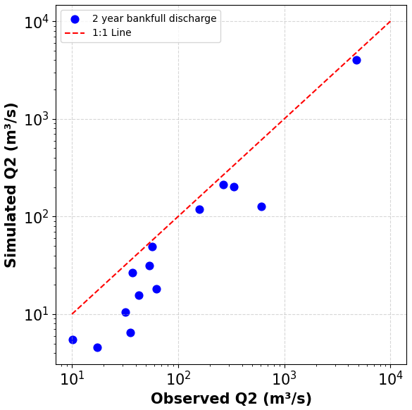
Figure 8 Observed vs. modelled 2-year Qbf, for river gauges in ten US basins. All points fall below the 1:1 line, which indicates a consistent low bias in the bathymetry.

3.6.3 The influence of the DEM input

This section explores how different DEMs were found to influence the performance of the SFINCS model in simulating flood extents. All simulations in this section are forced using GloFAS discharge, while only the DEM input is varied. We focused on two open-source DEMs with different spatial resolutions: FABDEM (30 m; Hawker et al., 2022) and 3D Elevation Program (3DEP; 1 m; USGS, 2015). The resolution of the SFINCS model was kept the same between the two different inputs, although we increased the level of detail (i.e. hypsometry levels, n=20, default 10) stored in the subgrid tables when using the 3DEP DEM. Both DEM inputs (FABDEM at 30 m and 3DEP at 1 m) are internally reprojected to the same SFINCS model grid resolution using hydromt. Therefore, the key difference lies not in the model grid resolution itself, but in the richness of the subgrid representation: higher-resolution DEMs provide more detailed elevation information within each grid cell, which is captured through the subgrid hypsometry tables. The same ten sub-basins in the United States were selected for this analysis based on the availability of 3DEP. However, vertical inconsistencies were observed in the original 3DEP dataset, where merging adjacent tiles sometimes introduced elevation differences of up to 3 metres. As a result, only six sub-basins were used in the final performance comparison. When using FABDEM, the average CSI was 0.37 across the six sub-basins. The mean CSI increased to 0.57 when using 3DEP DEM, which highlights the positive effect of higher-resolution elevation data on model accuracy. This improvement likely resulted from the finer spatial resolution of 3DEP and higher vertical accuracy. Moreover, 3DEP's 1 m LiDAR-derived DEM achieved a root mean square error of 0.53 m (USGS, 2022) compared to FABDEM's mean absolute vertical error reductions from 1.61 to 1.12 m in built-up areas and from 5.15 to 2.88 m in forests (Hawker et al., 2022).

Figure 9 illustrates the model's performance with these two DEMs in one of the six basins. Figure 9b shows the FABDEM dataset results, where the CSI was 0.46 for this particular basin. In this case, the lower-resolution DEM resulted in poorly defined river channels, especially in side streams, which prevented water from flowing accurately to downstream areas of the basin. In the upstream part of this basin, FAs were seen where water accumulated but could not reach the downstream areas. In contrast, when the 3DEP DEM was used (Fig. 9a), the model's performance improved significantly. A CSI of 0.59 showed a much better flow representation (i.e. fewer FAs in the upstream part), as the higher-resolution DEM allowed water to reach the downstream parts of the catchment. The increased detail in the terrain allowed for a more accurate representation of floodplains and channels (Jiang et al., 2022), which improved the HR while reducing the number of misses (red pixels) and FAs (yellow pixels).

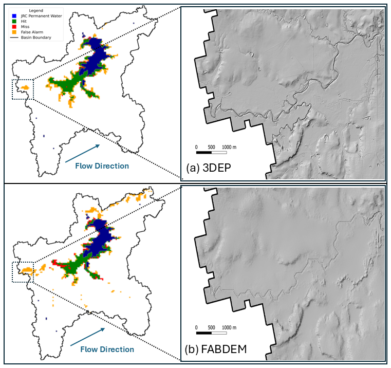
Figure 9 Influence of two DEMs on SFINCS performance: (a) 3DEP DEM of 1 m resolution and (b) FABDEM of 30 m resolution.

3.7 Cross-comparison and limitations

The global mean CSI of 0.39 of this study falls within the broad range reported by other large-scale flood modelling studies, but a clearer picture emerges when we distinguish between those studies using only modelled discharge and those incorporating observed streamflow. Studies driven exclusively by modelled discharges have tended to report lower skill. For example, in a global model intercomparison, Bernhofen et al. (2018) compared six global flood models against three historic African flood events and found mean CSI values of ∼0.4–0.7 for a 25-year flood. Likewise, Mester et al. (2021) used ten different global hydrological models to force the hydrodynamic model CAMAFlood and reported CSI values between 0.3 and 0.5 across eight historic flood events. Similarly, Dottori et al. (2022) used ERA5-driven discharges in LISFLOOD for ten flood events in Europe and obtained CSI values of 0.11–0.28 for high probability small events (<30 years) and 0.45–0.56 for large extreme events (>500 years). The SFINCS simulations using GloFAS discharge performed in this study (average CSI=0.39) align closely with these findings. In contrast, studies that make use of observed discharge data consistently achieved much higher performance. Wing et al. (2017) used the USGS National Elevation Dataset (1 arcsec or ∼30 m) and evaluated LISFLOOD against high water marks in 35 discrete US events using gauge records and reported a CSI of 0.87. Similarly, Hawker et al. (2024) combined field-measured discharges with remote-sensing extents in three Vietnamese case studies and obtained CSI values between 0.37 and 0.62. In this study, when SFINCS was forced with observed USGS discharges, the average CSI was 0.67 (HR=0.86; FAR=0.21), which shows the benefit of using accurate discharge inputs in hydrodynamic modelling. While such accuracy is currently best achieved with stream gauge observations, hydrological models capable of producing similarly accurate discharge estimates can deliver comparable results, especially given the sparse spatial coverage of gauges in many regions. Beyond discharge forcing, differences in DEM and bathymetric inputs also play an important role. The sensitivity analyses undertaken in this study show that using higher-resolution elevation data (e.g. 3DEP vs. FABDEM) and changing the bankfull return period to local conditions using observed streamflow data can significantly enhance model accuracy.

However, some differences and similarities exist in the setup and findings of our study compared to other large-scale modelling studies.

3.7.1 Number of events

Our study is unique in the high number (n=499) of events covered, which is much higher than in existing studies covering approximately 2 to 35 events (Risling et al., 2024; Wing et al., 2021; Bernhofen et al., 2018). Moreover, our study includes small upstream basins (<50 km²) to address the critical need to understand local upstream floods better. Hence, our model's performance has been assessed across a more diverse hydrological and geographical setting. Notably, we simulated multiple events with different timings and intensities in the same basin, which can be quite challenging to explain performance (Wing et al., 2021).

3.7.2 Hydrological forcing

The accuracy of hydrodynamic flood models (e.g. SFINCS) depends on the quality and characteristics of the hydrological drivers used as input. Previous studies have shown that the choice of hydrological forcing can strongly influence simulated flood extents. For example, a study by Mester et al. (2021) assessed the sensitivity of hydrodynamic models to hydrological forcings using ten different global hydrological models and eight case study areas with observed flood extent values. These basins were selected based on their relatively large size, as it was assumed that the relatively coarse hydrological models would not perform well for smaller sub-basins. Mester et al. found that the agreement between simulated and observed flood extents varied significantly across models and climate forcings. Moreover, Wing et al. (2021) found a CSI of 0.87 but used only observed hydrological forcing for their hydrodynamic model. It is well-known that global hydrological models perform poorly in smaller upstream basins due to their coarse resolution (e.g. Salinas et al., 2013; Mester et al., 2021), which could partly explain the poorer performance of the SFINCS model in these areas. We saw higher performance with SFINCS when it was supplied with observed discharges (CSI=0.67). The inability of the GloFAS hydrological model to capture the discharge peaks during a flood can significantly impact performance (Figs. 5d and 7a). This uncertainty in event discharge significantly impacts flood extent and likely explains much of the reduced CSI (0.39 globally; 0.67 when using USGS observations).

In our current setup, we saw that the bathymetry and river channel dimensions were underestimated (Sect. 3.6.2), which resulted in higher FAs because channel conveyance capacity was not represented correctly. The SWOT satellite mission provides high-accuracy measurements of water surface elevation, river width, and slope for rivers greater than 100 m in width (Neal et al., 2021; Larnier et al., 2020). Incorporating this dataset may improve flood modelling accuracy, particularly for river systems that have no data. In addition, using the “gradually varying solver” method to estimate river channel capacity, can replace the traditional Manning's equation. This method can also significantly improve bathymetry and flood inundation simulations (Wing et al., 2024). Neal et al. (2021) demonstrated the benefits of this approach in localised studies, and its application at the global scale may yield more accurate flood predictions.

3.7.3 Buffer

Another difference in our approach is the exclusion of permanent water bodies from the observed and simulated flood extent (250 m resolution), with no additional buffer applied around the rivers. This approach contrasts with methods used in other large-scale validation studies, such as Wing et al. (2017) and Dottori et al. (2022), which applied spatial buffers around the rivers to better capture floodplains and address benchmark data limitations. For example, Wing et al. (2017) applied a fixed buffer (i.e. ∼1 km around the rivers) to include areas potentially missed by benchmark data, particularly in small tributaries. Dottori et al. (2022) employed variable buffer zones (i.e. ∼5 and ∼10 km) tailored to account for diverse floodplain morphologies and the variable extent and density of the mapped river network. In our validation, we excluded permanent water using satellite-derived flood extent, so correctly simulated inundation in meandering and narrow channels (<250 m wide) was instead counted as an FA, even though these areas should be masked as permanent water. This misclassification inflated the FA ratio while decreasing the HR, which contributed to a lower average global CSI.

3.7.4 Uncertainties in validation data

As Tellman et al. (2021) noted, MODIS often fails to capture floods in rapid flash-flood events or under dense canopy cover, which leads to underestimation of true flood extents and contributes to lower CSI values. Additionally, cloud and snow cover can further obscure floodwaters, which adds to observational uncertainty. Some northern latitudes can have errors greater than 65 % in the flood detection algorithm due to the low sun angle on dark soil, which causes low reflectance that mimics water.

The comprehensive validation dataset relies on 250 m MODIS pixels, which limits the detection of narrow or small-scale inundation features and can misclassify flood zone delineation (Landwehr et al., 2024). Moreover, most binary pattern matching metrics are sensitive to the proportion of flooded area, meaning that large-scale floods are favoured while smaller-scale floods are less accurately reflected in the validation scores (Landwehr et al., 2024). Binary flood extent masks and class-based metrics (e.g. the CSI) do not account for important factors such as flood depth and its influence on impacts and model accuracy (Stephens et al., 2014). As a result, some of the poorer performance in smaller basins likely reflects limitations in the reference dataset and validation framework rather than shortcomings in the hydrodynamic model.

3.7.5 Flood protection

Although studies on global flood protection standards exist (e.g. Scussolini et al., 2016), incorporating more accurate data on flood protection standards into future global flood models should be considered. Previous research, including studies by Mester et al. (2021), has shown that flood protection can influence model performance by increasing variability, though it does not necessarily change the maximum performance scores. Further exploration into this area may provide valuable insights into how flood protection measures impact flood risk across regions.

4 Conclusions and Recommendations

Our study evaluated the performance of the SFINCS model in simulating 499 riverine floods globally. Our findings show that the model can simulate riverine flood extents globally, with a mean CSI of 0.39 using GloFAS modelled discharges as input forcing. However, performance improved considerably when using observed discharge inputs. It reached a CSI of 0.67 across ten US events, which highlights the considerable value of in-situ hydrological observations for model accuracy. Furthermore, using a higher-resolution DEM (3DEP, ∼1 m) improved the mean CSI from 0.37 (FABDEM, ∼30 m) to 0.57. Conversely, a lower-resolution DEM resulted in poorly defined river channels, especially in side streams, which prevented water from flowing accurately to downstream areas.

The model accuracy substantially improved for larger upstream basin sizes. Specifically, simulations in basins with very large upstream areas (≥1000 km²) achieved an average CSI of 0.42, whereas those with small upstream areas (<50 km²) had an average CSI of 0.29. Sensitivity analyses further showed that model accuracy was sensitive to the quality of input data. For example, the GEB hydrological model outperformed GloFAS in selected regions, likely due to its finer spatial resolution (∼1 km²) and more realistic hydrographs.

Bathymetric calculations revealed a systematic low bias in the default return period estimates used in the global analysis, which are critical for defining realistic channel geometry. This underestimation propagated into narrower and shallower channel representations that reduced conveyance capacity while likely inflating flood extents during high-flow conditions.

These findings suggest that the SFINCS model is highly suitable for modelling river floods. Nevertheless, model accuracy can be improved through targeted enhancements in both hydrological and topographic inputs. Future research can explore methods to regionalise or dynamically calibrate bankfull return periods using observed discharge records where available (e.g. USGS or GRDC) rather than applying a fixed global default. A combined approach that uses long-term gauge data with emerging global remote sensing products (e.g. the SWOT dataset) can allow for more accurate bathymetric representation while reducing systematic biases in large-scale flood simulations.

Our cross-study comparison also confirmed that methodological choices (e.g. DEM resolution), bathymetric assumptions, and masking permanent water affect accuracy and comparability. For example, our decision not to apply spatial buffers or include permanent water bodies may have contributed to more conservative performance metrics, but the choice reflected a stricter and more objective comparison with satellite-derived flood extents. Future research may build on this decision by standardising validation approaches and testing the effect of different masking strategies, such as permanent water removal from reservoirs and the bankfull width of the rivers. The dataset used for validation, 250 m resolution MODIS-based flood maps, cannot detect narrow or meandering channels, particularly in smaller basins. Future large-scale research can prioritise integrating higher-resolution observational datasets such as Sentinel-1 Synthetic Aperture Radar (∼10 m), which can capture finer floodplain dynamics and provide real-time images multiple times during the day.

While the CSI provides good insight into the model's performance, it does not capture the vertical accuracy of flood simulations. As Wing et al. (2021) emphasised, incorporating flood depth can offer a more comprehensive evaluation, particularly for identifying errors in floodplain dynamics and understanding biases in inundation extent. Additionally, the upscaling of SFINCS results from 30 to 250 m resolution (to match our observed data) caused a loss of details that further impacted model performance. The findings of this study echo research that calls for better open-source observed flood validation datasets, such as the Global Flood Monitoring System offered by Copernicus Emergency Management Service (Salamon et al., 2021; Wagner et al., 2026; Bates, 2023). We recommend the development of standardised, large-scale validation frameworks including agreed masking protocols, and using both simulated and observed discharges so that future studies can be directly compared.

Appendix A

A1 Bathymetry

Bathymetry, the measurement of the depth and width of rivers, is one of the most challenging variables to estimate on a global scale due to the lack of comprehensive, high-resolution data, particularly in remote or unsurveyed regions (Dey et al., 2019). Accurate representation of river bathymetry is critical for hydrodynamic modelling, as it directly influences the conveyance capacity of rivers and channels, which affects flood inundation predictions (Wing et al., 2024). We simulated bathymetry with the following steps.

A1.1 Step 1. Matching River Centerline and Discharge Data

The process began by clipping the river centerline vector dataset (MERIT-SWORD) to the model domain (flooded MERIT-BASINS + additional downstream basin) with a small buffer. Then, we matched the individual river segments to the global hydrological model GloFAS using upstream area data. The matching used the origin points of each river segment, which were snapped to a particular upstream area pixel in the GloFAS dataset using the HydroMT package. When snapping points to the discharge grid, this package considers a 5 % relative error tolerance and a 50 km² absolute error cap. The upstream area was a key indicator of river flow and helped to identify the centerline segments corresponding to different river sections. This step ensured that discharge calculations were correctly linked to the appropriate locations on the river. Once the river segments were matched, we extracted discharge values focused on the yearly discharge maxima from 1979 to 2024. These maxima formed the basis for our return-period analysis via the block-maxima method, which selected the single largest discharge value each year (45 years).

A1.2 Step 2. Utilising PyExtremes for Distribution Analysis of Discharge Data

Next, we used the PyExtremes Python package (https://georgebv.github.io/pyextremes/, last access: 16 January 2025) to fit the yearly discharge maxima to an appropriate distribution. PyExtremes helped to determine the best fit for the maximum discharge values, which might follow different distributions for extreme value analysis. The distribution selection was based on the characteristics of the discharge data (from GloFAS) to ensure that we accurately captured the probability of various discharge levels. Using these fitted distributions, we calculated discharge values for different return periods. We used a 2-year return period discharge, a typical proxy for bankfull discharge (e.g. Wilkerson, 2008). Bankfull discharge refers to the flow level at which the river is filled to the top of its banks without overflowing, a key indicator for estimating the river's cross-sectional shape. To compute return periods, the package ranks extreme values, calculates exceedance probabilities, and derives return periods as multiples of a specified return period size (typically one year). This systematic approach allowed it to assign empirical return periods to the extreme values extracted from our discharge data.

A1.3 Step 3. Estimating Bankfull Width and Depth

Only global river segments 30 m wide and greater are represented in the SWORD database (Altenau et al., 2021). Thus, the river centerline vector dataset MERIT-SWORD is missing river-width values for river segments smaller than 30 m (https://doi.org/10.5281/zenodo.14675925, Wade et al., 2025). To estimate the bankfull width of the rivers (<30 m), we applied a power-law relationship that linked discharge to channel width, based on empirical studies (Leopold and Maddock, 1953). The power-law formula allowed us to predict the width based on the bankfull discharge calculated earlier.

$$W=a\cdot Q^b$$

where W is the bankfull width,Q is the bankfull discharge (from the 2-year return period), a and b are empirically derived constants

Once the width was estimated, we proceeded to calculate the bankfull depth for all the river segments in the model domain. Depth was estimated by applying Manning's equation for open channel flow, which relates the river's flow velocity, roughness, and channel geometry (including slope and depth) to its discharge. Manning's equation is expressed as follows:

$$Q={\displaystyle \frac{\mathrm{1}}{\left(n\right)}}\cdot A{R}^{\left(\frac{\mathrm{2}}{\mathrm{3}}\right)}\cdot S^{\left(\frac{\mathrm{1}}{\mathrm{2}}\right)}$$

where Q is the discharge, n is the Manning's roughness coefficient, A is the cross-sectional area, R is the hydraulic radius (cross-sectional area divided by wetted perimeter), S is the slope of the river.

A2 Hydro-MT and Snakemake

A2.1 Hydro-MT (Eilander et al., 2023a)

HydroMT is an open-source Python package designed to streamline the process of building and configuring water system models (e.g. SFINCS). The framework handles various spatial data types, including gridded raster data like DEMs and vector data like shapefiles. It automates essential steps in the preprocessing, setup, and postprocessing of hydrodynamic models, so it is a versatile tool for hydrological modelling.

The HydroMT-SFINCS sub-package, specifically tailored for the SFINCS model, extends the core HydroMT functionalities to address the specific needs of SFINCS users. One key function of HydroMT-SFINCS is the configuration of boundary conditions, which includes integrating inflow and outflow boundary conditions for rivers, setting up forcing conditions (e.g. hydrographs and precipitation), and defining external water level boundaries. The sub-package also generates a mask for active and inactive cells based on the basin boundary. Thus, we ensured that our calculations were carried out only in relevant flood-prone areas while excluding regions unaffected by flooding.

HydroMT-SFINCS is also adept at handling and converting input data from various formats (e.g. NetCDF, GeoTIFF, and shapefiles) into the structure required by the model, which includes preparing static input layers (e.g. DEMs, land-use maps, and basin boundaries) in a unified format. The tool ensures spatial consistency across different datasets through automated reprojection, resampling, and cropping to minimise potential errors that can arise from manual data processing.

Regarding postprocessing, HydroMT-SFINCS automated the interpolation of SFINCS output, which was stored as NetCDF files containing water levels for each subgrid cell. For each time step, these water levels were interpolated onto the DEM data to produce water depths, which were then used to generate the maximum flood extent. By automating the pre- and postprocessing steps, HydroMT-SFINCS minimised the risk of errors and significantly accelerated the model setup and output generation process. This approach enabled the rapid testing of various model configurations and ensured reproducibility, which is especially important for large-scale and scenario-based modelling studies.

A2.2 Snakemake (Mölder et al., 2020)

Snakemake is a workflow management system designed to handle complex data analysis pipelines in a reproducible and scalable manner. It is particularly useful in scientific computing, where numerous tasks and steps must be executed in a specific order to ensure the efficient processing of large datasets. Snakemake uses a simple syntax to define rules for data processing, where each rule specifies input files, output files, and the command to execute.

In our workflow, Snakemake was used to automate and streamline the processing of all flood modelling tasks, from preprocessing to validation. By organising each task into separate rules, Snakemake enabled the reproducibility of the entire process. The flexibility of Snakemake allowed us to easily parallelise tasks, for example, by running multiple model domains (i.e. clusters) for the same event simultaneously on different computing nodes. This ability expedited the analysis while making it easier to handle large-scale simulations. Hence, the results were generated in a timely manner. For example, events were split and executed in parallel across multiple compute nodes equipped with AMD EPYC 9354P processors (64 CPU cores, 96 GB RAM per node). Based on Snakemake log files, the average wall-clock time for a single basin simulation was approximately 7 min for a ∼1000 km² domain and a typical simulated flood period of ∼30 d.

Each flood event consists of multiple basin cluster simulations (on average ∼30 per event), resulting in a large number of individual simulations across the full dataset. These simulations were executed in parallel; however, the overall workflow also includes sequential steps per event (e.g. model setup, forcing update, simulation, and post-processing), as well as I/O and scheduling overhead. As a result, the total elapsed wall-clock time for completing all simulations was approximately 44 d. By integrating Snakemake into our modelling pipeline, we ensured that each step of the analysis, from data preprocessing to final flood map and validation, was reproducible and easily adjustable for future adjustments or expansions of the study.

A3 Effect of Protection Standards on Model Performance

A key limitation of global flood modelling frameworks is the inability of global DEMs to capture flood protection structures such as embankments and levees along river channels (Dottori et al., 2022). In this study, the modelled framework makes use of FABDEM (Hawker et al., 2022) and the floodplains are simulated using the subgrid approach. While subgrid methods have been shown to improve the representation of floodplains (Reshma et al., 2024), they still rely on the underlying DEM and therefore do not specifically take into account flood protection structures. To explore the effect of the protection standards on the model performance we make use of the FLOPROS dataset (Scussolini et al., 2016), which provides regional protection levels in terms of return period. Using this dataset, we assign flood protection standards (in return period years) at sub-national administrative level. As flood events can occur over a large area, we look at each basin cluster separately and assign values from the FLOPROS database. Some events occurring predominantly in low-income regions or smaller countries could not be assigned a protection level and were excluded from this analysis. The analysis was conducted in 4 key regions (North America, Europe, Africa, and South America). The results show consistent differences between regions, and the regions with higher protection standards (Europe and North America) show relatively higher bias values (1.12 and 1.26, respectively), indicating a tendency of the model to overestimate flood extent. In contrast, less well protected regions (South America and Africa) show lower bias values (0.96 and 0.89, respectively), suggesting more balanced or slightly underpredicted flood extents.

These differences can be explained by both the absence of flood protection structures in the DEM and regional variations in hydrological forcing. In highly engineered regions such as Europe and North America, levees and embankments are not represented in global DEMs (Dottori et al., 2022), leading to overestimation of flood extent. In contrast, in less protected regions, floodplain processes are closer to natural conditions, which can reduce this source of overprediction.

In addition, differences in hydrological model performance may also contribute to the observed patterns. Alfieri et al. (2013) showed that GloFAS discharge simulations perform well in river systems such as the Amazon and Mississippi but exhibit limitations in semi-arid regions (e.g. the Niger), where processes such as evaporation and infiltration are not fully captured. This can affect the accuracy of simulated floods and may contribute to regional differences in model performance observed in this study.

Table A1 Model Performance grouped per region.

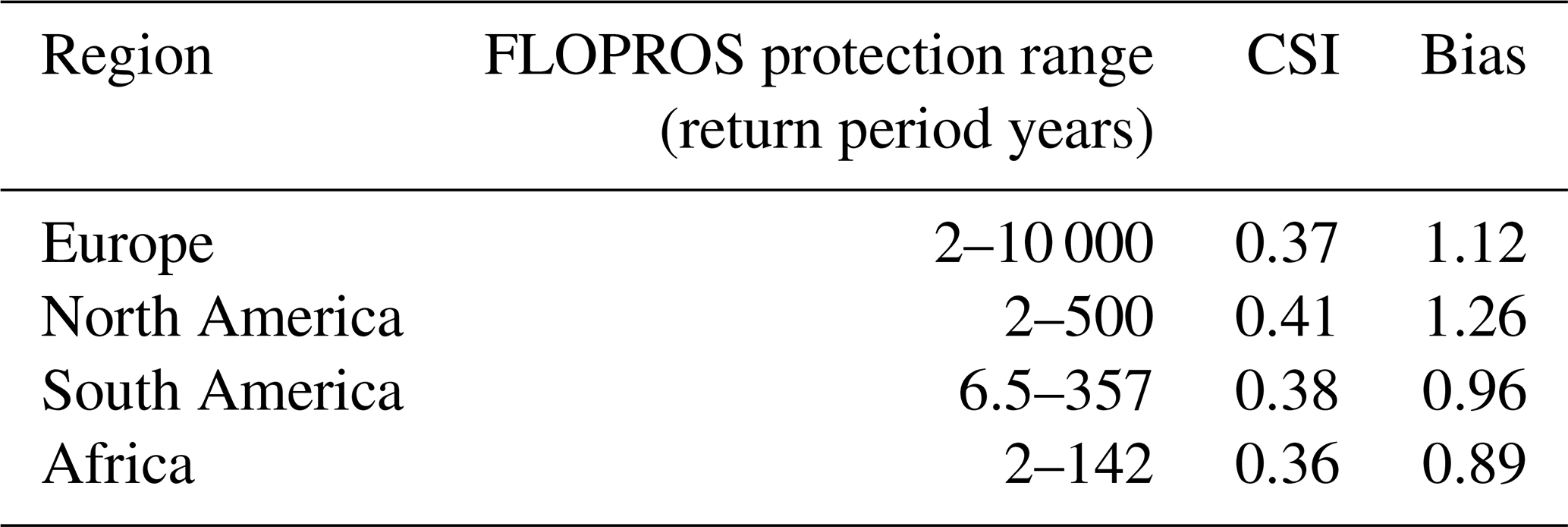
A3.1 Additional Figures

Figure A1 Section 3.1.1 Fig. 5d supporting argument figure.

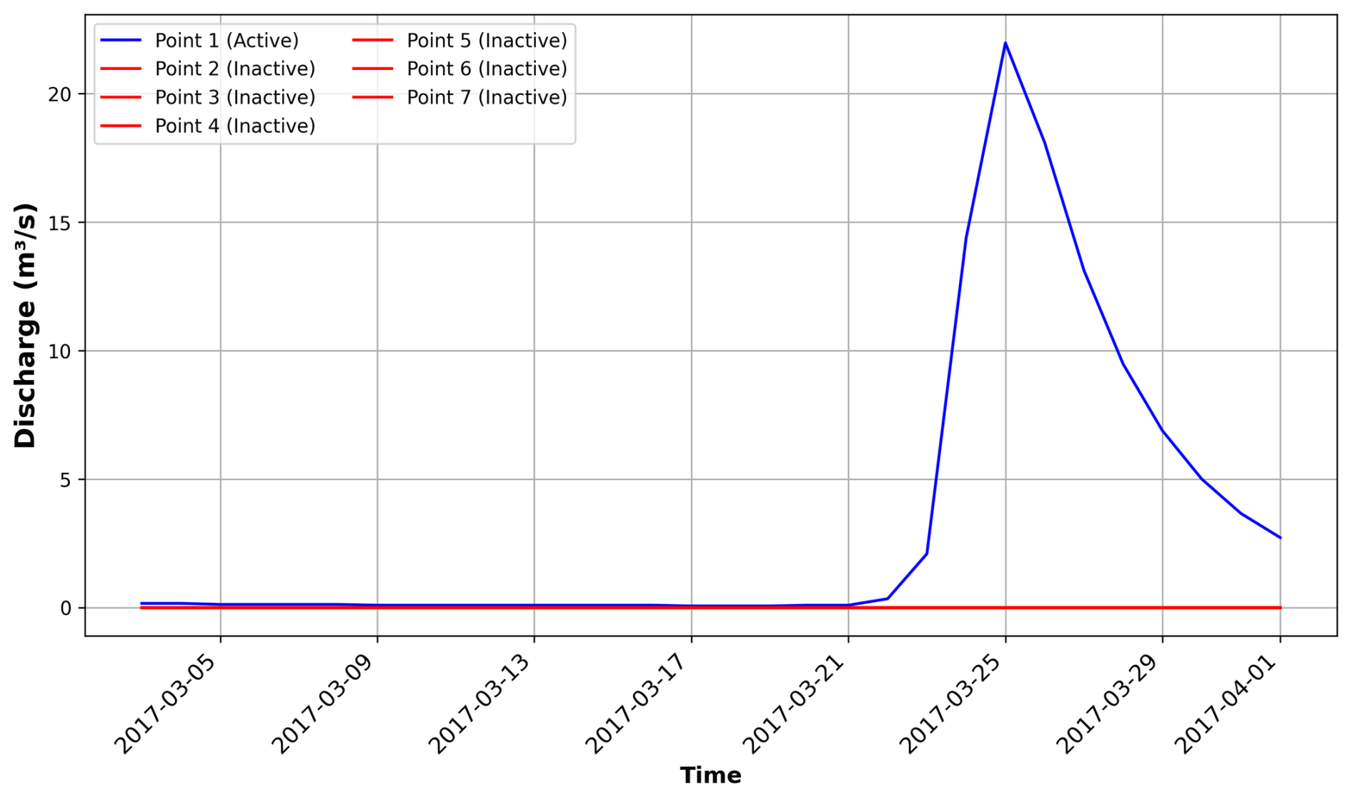
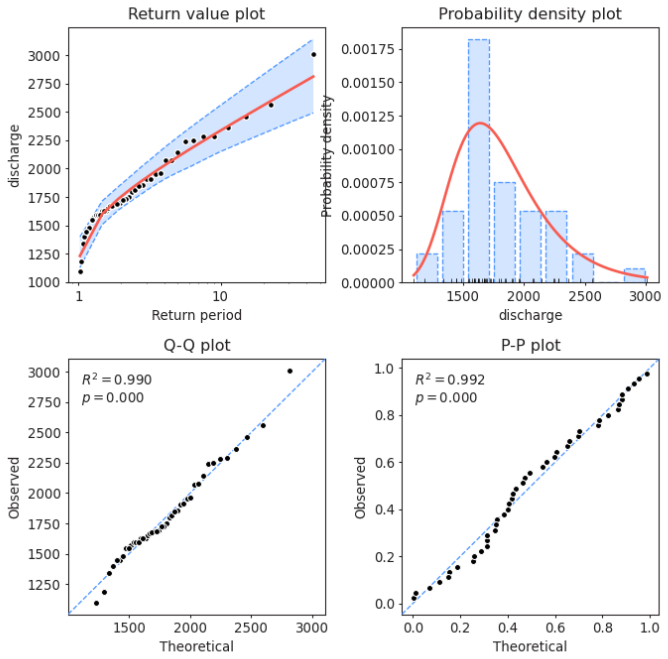
Figure A2 Example return period calculations “PyExtremes”, which were conducted for every river segment in the MERIT-BASINS dataset.

Figure A3 Observed vs. modeled 1.5-year Qbf, for river gauges in ten U.S basins.

Figure A4 Observed vs. modeled 2.5-year Qbf, for river gauges in ten U.S basins.

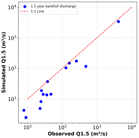
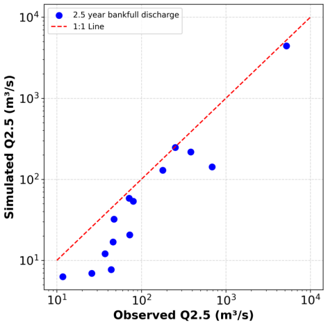
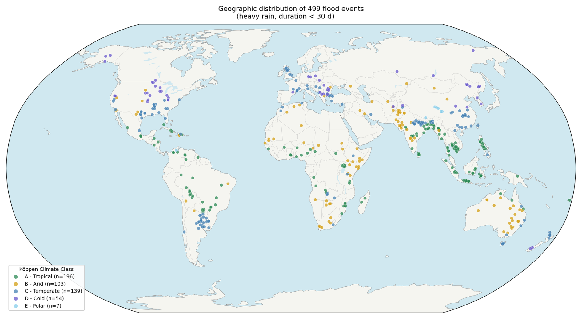
Figure A5 Modelled flood events filtered from the Global Flood Database with respect to their Koeppen Climate Zones.