Process diagnostics of snowmelt runoff in global hydrological and land surface models – Part 1: A systematic evaluation across basins of increasing complexity

Accurate simulation of snowmelt runoff (SMR) is critical for water resource management. However, despite the abundance of global hydrological models, little is known about their SMR performance. This study presents a comprehensive evaluation of SMR across 15 state-of-the-art large-scale models and runoff products by focusing on their biases in first-order indices, i.e., the total volume (Q_sum), peak flow (Q_max), and centroid timing (CTQ) of runoff in the snowmelt period. Then by introducing 1455 snow-dominated basins with diverse topography and vegetation complexities, we further proposed a novel model robustness metric to test how different models perform under increasing basin complexity, thereby allowing for a quantification on how they adapt to complex environmental conditions. Our results reveal that (1) most models exhibit underestimated Q_sum and Q_max and predict CTQ too early. These biases are particularly pronounced in regions such as the western United States, northern Europe, and northeastern China. (2) Model biases systematically increase with basin complexity, with CTQ exhibiting strong sensitivity to mean elevation and topographic variability, while Q_sum and Q_max being shaped more by mean elevation and the diversity of vegetation types in the basin. (3) The robustness assessment further shows that observation-constrained runoff products exhibit the most outstanding performance (i.e., low biases and strong adaptability to stern conditions), followed by the hydrological and land surface models. Notably, while global hydrological models generally exhibit stronger robustness in simulating Q_sum and Q_max, land surface models show a clear advantage in simulating CTQ, highlighting their structural strength in capturing melt timing rather than runoff magnitude. This study provides a large-sample benchmark for SMR evaluation and complements existing model assessment approaches by examining model performance across basin complexity gradients, offering useful insights for future model development and uncertainty reduction.

1 Introduction

Snowmelt runoff (SMR) is a critical freshwater resource supporting human society and agricultural development. Globally, SMR contributes approximately 50 % of the annual runoff for more than 26 % of the terrestrial land area, directly supplying freshwater for about one-sixth of the world's population (Qin et al., 2020). Accurate simulation of SMR is therefore essential for effective water resources management and for assessing the impacts of climate change on water resources. This need becomes increasingly urgent under future climate change scenarios, where established snow–runoff relationships are expected to shift substantially (Wieder et al., 2022), necessitating a systematic understanding of SMR dynamics.

However, although large scale hydrological models have been widely used to simulate SMR in cold region hydrology, accurately reproducing key SMR characteristics across diverse basin conditions remains challenging. This challenge is partly related to the coupled nature of SMR-related processes, including rainfall–snowfall partitioning, sublimation, canopy interception, and snowmelt dynamics, as well as to uncertainties in forcing data, parameterization (Lei et al., 2025), and model structure. Such a challenge is consistently highlighted by multi-Model Intercomparison Projects (MIPs). For example, Hou et al. (2023) reported substantially lower model skill in cold regions compared to non-cold regions. Similarly, Guo et al. (2024) revealed markedly larger runoff biases in cold regions, particularly for extreme events. However, existing model assessments have largely emphasized the overall model performance at annual or seasonal time scales (Tang et al., 2023), and comprehensive evaluations explicitly targeting SMR remain rare. These studies generally attributed errors to simplified process representations, parameter uncertainties, or model structures (Beck et al., 2017; Haddeland et al., 2011), without a direct diagnosis of the underlying processes. As a result, the critical deficiencies in SMR processes are usually entangled with errors from other hydrological processes (Chai et al., 2025), compromising our understanding of the behavior and limitations of existing models. This highlights an urgent need for a tailored diagnosis for the SMR processes to guide future model development.

One of the key factors of a systematic assessment is to identify the appropriate evaluation perspectives. Previous model evaluations have primarily focused on aggregated metrics such as the Nash–Sutcliffe Efficiency (NSE; Nash and Sutcliffe, 1970) and the Kling–Gupta Efficiency (KGE; Gupta et al., 2009). While they are useful for assessing the overall temporal dynamics, their aggregated nature makes it difficult to disentangle the specific deficiencies tied to process representations. In fact, a satisfying model should accurately capture the major characteristics of the SMR hydrograph, namely its total volume (Q_sum), peak flow (Q_max), and centroid timing (CTQ), which are the first-order metrics crucial to water resource management and utilization. However, past assessments have not been structured to explicitly quantify these dimensions, which may hide the potential trade-offs of certain models (e.g., a model excelling in timing but failing in volume).

Beyond the major characteristics of a hydrograph, a more critical perspective is to assess how well a model performs across diverse land conditions. This is particularly relevant for SMR simulation, where land surface complexity is known to challenge model accuracy. The complexity is generally related to terrain and vegetation conditions (Li et al., 2022; Fenicia et al., 2014): high-elevation environments introduce intricate rainfall–snowfall partitioning thresholds and enhanced sublimation (Schulz and De Jong, 2004; Strasser et al., 2008), while varied topography and vegetation demand sophisticated representations of canopy interception, radiation transfer, and runoff generation. Taken together, a model that performs well or maintains its skill even in the face of increasingly complex land surface conditions should be considered robust. However, past assessments have rarely been designed to test this robustness and reveal which type of models excel under varying levels of complexity. This presents another gap in benchmarking our current modeling capabilities.

To address these gaps, we gathered 15 state-of-the-art large-scale runoff models and data products across 1455 snow-dominated basins worldwide for the period 1979–2019. Based on this dataset, we systematically evaluated their SMR performance by explicitly considering the three primary characteristics of the SMR hydrograph, followed by a further test of model robustness using a novel metrics to describe the performance under varying land complexities. The models and products include six Inter-Sectoral Impact Model Intercomparison Project (ISIMIP2a) water-sector models (PCR-GLOBWB, DBH, VIC, MATSIRO, CLM40, LPJML), seven ISIMIP3a water-sector models (CWATM, H08, HYDROPY, JULES-W2, MIROC-INTEG-LAND, ORCHIDEE-MICT, WATERGAP2-2E), and two recent global river-flow data products, namely Global Reach-Level A Priori Discharge Estimates for Surface Water and Ocean Topography (GRADES; Lin et al., 2019) and Global River Discharge Reanalysis (GRDR; Feng and Gleason, 2024a). Our model selection criteria are twofold: first, it should cover a sufficiently wide spectrum of models to facilitate a discussion on the performance and process disparities of different modelling schemes (Chen et al., 2021; Guo et al., 2024; Hou et al., 2023); second, it should cover observation-constrained runoff products, allowing for an assessment of the potential performance gains from gauge or satellite data. Our analysis begins with a systematic assessment of the primary characteristics of SMR (total volume, peak flow, and centroid timing), followed by an analysis of performance stratified by basin complexity and a detailed discussion of model robustness. By combining multiple SMR characteristics with model robustness analysis across basin-complexity gradients, this study aims to provide a complementary perspective for diagnosing model deficiencies and informing future model development and uncertainty reduction.

2 Data and Methods

2.1 Data

2.1.1 ISIMIP2a/3a water sector models and global runoff products

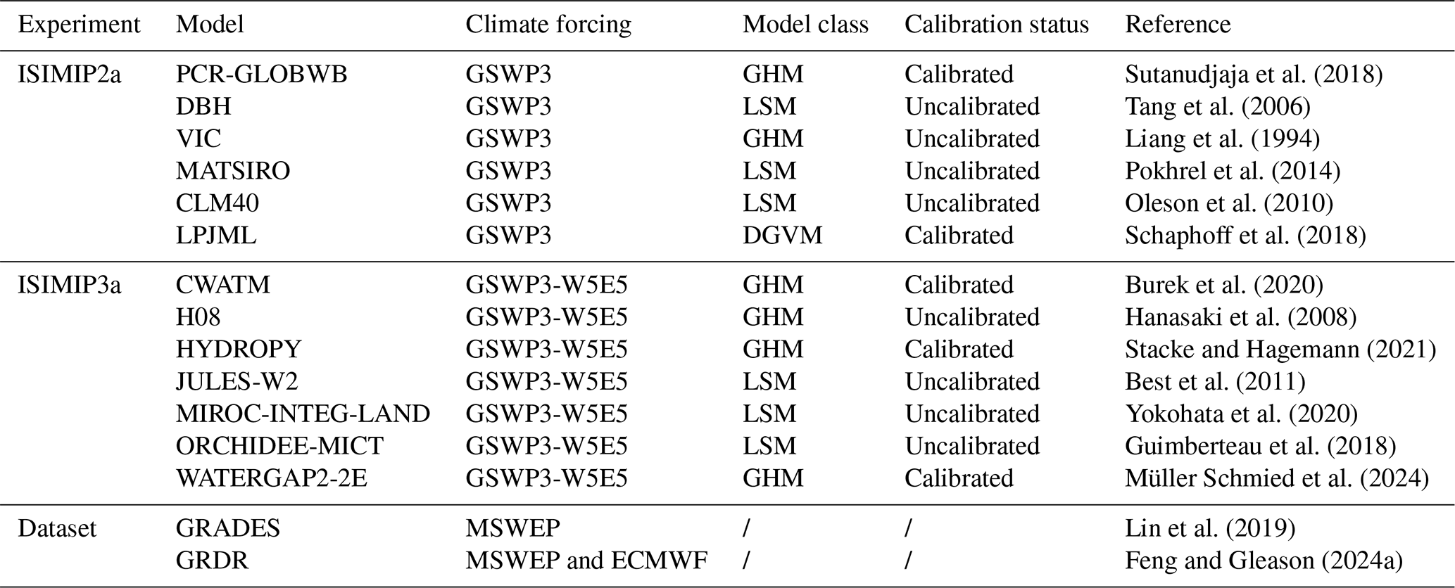
Table 1 summarizes the 13 state-of-the-art macro-scale water sector models and two data products utilized in this study. Among these, six models belong to ISIMIP2a, while seven are part of ISIMIP3a. All models were obtained from the ISIMIP water sector data repository (https://data.isimip.org/, last access: 19 November 2024). For each model, their total runoff (i.e., sum of surface and subsurface runoff) was extracted for river routing (Sect. 2.2), and the key SMR indices were subsequently calculated for evaluation (Sect. 2.3).

These models were categorized into three groups (see Table 1 and references therein): i.e., six global hydrological models (GHMs: PCR-GLOBWB, VIC, CWATM, H08, HYDROPY, and WATERGAP2-2E), six land surface models (LSMs: DBH, MATSIRO, CLM40, JULES-W2, MIROC-INTEG-LAND, and ORCHIDEE-MICT), and one dynamic global vegetation model (DGVM: LPJML). We categorized the models into these groups primarily because GHMs tend to focus on water balance representation, LSMs are generally more advanced in simulating energy-exchange processes, and DGVMs are better suited for capturing vegetation ecosystem dynamics. Thus, comparative analyses across different model categories may provide insights into their relative strengths and limitations. We also included two observation-constrained datasets for evaluation – GRADES, a global runoff product based on VIC model simulations followed by bias correction using gauge-extrapolated information, and GRDR, a recently released global runoff product that enhances accuracy by assimilating river-width data from Landsat into a model-based discharge simulation framework. Incorporating these two discharge products allows for discussions on the gains brought by observational constraints.

Because parameter calibration can influence runoff simulation, especially for runoff magnitude and peak flow, we further documented the calibration status of the evaluated models based on the available model documentation and calibration information. Five models, including PCR-GLOBWB, LPJML, HYDROPY, CWATM, and WATERGAP2-2E, were classified as calibrated models, whereas MATSIRO, DBH, CLM40, MIROC-INTEG-LAND, VIC, ORCHIDEE-MICT, JULES-W2, and H08 were grouped as uncalibrated models because no explicit calibration entry was available in the original model information.

All models were run at a spatial resolution of 0.5° with daily time steps. Models with similar meteorological forcing and simulation scenarios were purposefully chosen such that our comparisons more directly focus on process diagnostics, although other uncertainty sources such as calibration differences, forcing uncertainty, and model-specific implementation choices cannot be fully eliminated. All models and datasets were matched to the same geospatial framework (i.e., the MERIT-Basins river network; Lin et al., 2019) to ensure consistency. Further details are provided in Sect. 2.2.

Sutanudjaja et al. (2018)Tang et al. (2006)Liang et al. (1994)Pokhrel et al. (2014)Oleson et al. (2010)Schaphoff et al. (2018)Burek et al. (2020)Hanasaki et al. (2008)Stacke and Hagemann (2021)Best et al. (2011)Yokohata et al. (2020)Guimberteau et al. (2018)Müller Schmied et al. (2024)Lin et al. (2019)Feng and Gleason (2024a)

Table 1 Overview of models and data products considered in this study. Calibration status indicates whether explicit calibration information is available from the original model documentation or related model information. Models without explicit calibration information are grouped as uncalibrated in this study.

2.1.2 Routing runoff with the RAPID vector-based routing model

To ensure that all models are comparable under the same geospatial framework, we first routed the gridded runoff of all ISIMIP2a and ISIMIP3a models through the same river routing model, RAPID (the Routing Application for Parallel computatIon of Discharge; David et al., 2011). RAPID is an efficient vector-based river routing model that enables intercomparison of discharge at global scales (David et al., 2011), making it an ideal choice for routing ISIMIP runoff.

The river network used for routing is MERIT-Basins (Lin et al., 2019), a high-resolution, vector-based hydrography dataset constructed from the MERIT-Hydro DEM (Yamazaki et al., 2019). We use the area-weighted mapping technique (Lin et al., 2018) to map the gridded runoff (0.5°) onto the vectorized hydrography to determine lateral inflows, with the connectivity of the river-network topology pre-specified as input. RAPID employs the Muskingum method, which requires two parameters: a weighting factor x and the flood-wave travel time k. Since x is less sensitive in the Muskingum method, it is typically set to 0.3 globally. In contrast, k plays a key role in routing performance and is estimated using river-specific characteristics. Specifically, k is calculated for each river reach by combining channel length with flow celerity estimated from Manning's equation, as expressed in Eq. (1):

$$\begin{array}{}\text{(1)}& k={\displaystyle \frac{\mathrm{3}\ln }{\mathrm{5}\sqrt{S_{\mathrm{0}}}{\left(\frac{wd}{\mathrm{2}d+w}\right)}^{\mathrm{2}/\mathrm{3}}}}\end{array}$$

Where l is the length of the river channel, n is Manning's roughness coefficient and is typically set to 0.035 for natural rivers (Lin et al., 2019). S₀ is the channel slope, and w and d are the river width and depth estimated by multi-year average runoff using a long established power-law equation (Andreadis et al., 2013). Note that the choice of river routing model and its parameters can influence both the timing and magnitude of SMR, particularly for Q_max and CTQ, which are more sensitive to runoff concentration pathways and travel-time estimates than Q_sum. In addition, a scale mismatch exists between the 0.5° gridded runoff outputs and the finer MERIT Basins river network used for routing. Although the area weighted mapping method and the consistent RAPID routing framework improve comparability across models, they cannot fully resolve subgrid heterogeneity or the allocation of coarse grid runoff to fine river reaches. This mismatch may introduce uncertainty into the absolute evaluation of basin scale runoff characteristics. Nevertheless, because our analysis focuses primarily on long-term mean SMR characteristics and applies the same routing procedure to all models and datasets, we expect this uncertainty to have a limited influence on the relative inter-model comparison. In summary, we standardized the forcing data, geospatial framework, and routing scheme as much as possible to improve inter-model comparability and to focus the evaluation more directly on differences in land model parameterizations and process representations. Nevertheless, forcing and routing-related uncertainties may still affect the simulated SMR characteristics, particularly Q_max and CTQ, and thus should be considered when interpreting both the absolute model performance and inter-model differences.

2.2 Methods

2.2.1 Definition of key SMR characteristics

As briefly discussed in Sect. 1, diagnosing processes related to SMR can be challenging due to the many processes involved (Fig. 1a). To simplify this, we focus on three first-order characteristics–total runoff (Q_sum), peak flow (Q_max), and the centroid timing (CTQ) of runoff in the snowmelt period. Q_sum is closely linked to water availability, Q_max determines flood hazard potential, and CTQ provides essential information for water resource management. More importantly, these metrics are directly linked with snow accumulation and melt processes (Fig. 1b). Specifically, rainfall–snowfall partitioning controls the precipitation phase and the magnitude of snow accumulation, while snow interception and sublimation regulate snow redistribution and loss. Together, these processes determine the amount of meltable snow, thereby influencing both Q_sum and Q_max. In comparison, the melt process, being more closely linked to energy dynamics, governs the timing and rate of SMR and exerts a stronger control on CTQ (Fig. 1b). Compared with a full time-series analysis, our focus on these key runoff characteristics offers a more direct and physically interpretable evaluation of model performance.

To obtain these metrics, we first defined the snowmelt period using snow water equivalent (SWE) data from the fifth-generation atmospheric reanalysis of the European Centre for Medium-Range Weather Forecasts (ERA5; Hersbach et al., 2020). Specifically, the snowmelt period was defined as the interval from the date of maximum SWE to the date when SWE dropped below 1 mm (Fig. 1c). This definition was designed to identify the dominant seasonal snowmelt period in a consistent manner across all basins, rather than to capture every short-term snowmelt-related runoff event. Therefore, it may not fully represent complex melt dynamics such as multi-peak melt seasons, intermittent melt–refreeze cycles, or rain-on-snow events. Here, ERA5 SWE was used mainly to identify the timing window of the main snowmelt period rather than to evaluate SWE magnitude. We acknowledge that ERA5 SWE contains uncertainties, especially in complex terrain where snow accumulation and melt are affected by elevation gradients, slope, aspect, vegetation cover, and sub-grid snow redistribution processes. However, their influence on the extracted SMR characteristics is expected to be limited, because this study focuses on the dominant seasonal snowmelt signal rather than short-term melt events or daily SWE variability. Moreover, Q_sum, Q_max, and CTQ were derived as long-term mean characteristics across multiple years, which reduces the sensitivity of the results to occasional errors in snowmelt-period boundaries. Therefore, although ERA5 SWE uncertainty should be considered, it is unlikely to substantially alter the main runoff characteristics used in this global scale evaluation.

After this, Q_sum is defined as the total runoff in the snowmelt periods. Q_max is the maximum discharge in the snowmelt periods. CTQ refers to the calendar date on which cumulative runoff reaches 50 % of the total runoff in the snowmelt period, which measures the timing of concentrated runoff during snowmelt, reflecting both the onset and the rate of melt. These definitions are conceptually consistent with previous studies that examined annual (Han et al., 2024) or cold-season runoff (Dudley et al., 2017), but they are further restricted to the snowmelt period to increase the SMR signals. We also introduced a few filtering steps to ensure the SMR signals are the dominant ones, which will be introduced in Sect. 2.2.2.

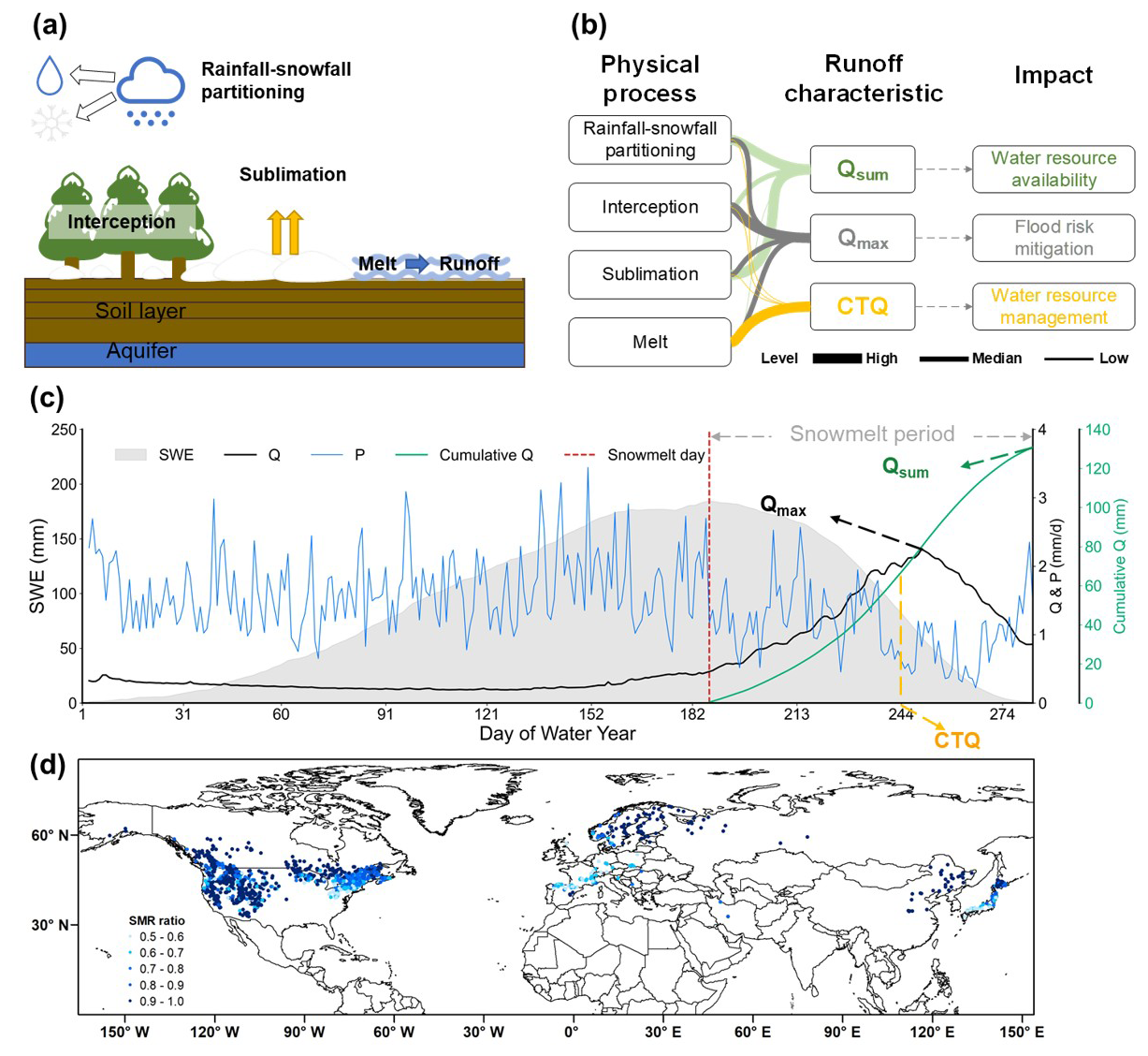
Figure 1 Major physical processes influencing snowmelt runoff (SMR), key runoff characteristics, and the study area. (a) dominant physical processes during snow accumulation and melt; (b) linkages between physical processes and key runoff characteristics; (c) definition of the snowmelt period and the three key characteristics used for model evaluation; (d) spatial distribution of hydrological stations and the ratio of snowmelt runoff.

2.2.2 Catchment selection

We obtained daily streamflow data from 1455 gauges (Fig. 1d) for evaluation. The gauge selection and associated catchment information were based on the Global Streamflow Characteristics, Hydrometeorology, and Catchment Attributes dataset (GSHA; Yin et al., 2024), which covers 21 568 gauges. We note that the public GSHA release provides annual and monthly streamflow indices, while the daily discharge time series were obtained through following the GSHA data retrieving packages, and the data were used to calculate Q_sum, Q_max, and CTQ. The gauges were then filtered to include only those above 30° N (i.e., mid- to high-latitude regions) and those with long-term snow water equivalent (SWE) ≥1 mm in at least one month of the cold season (i.e., during October to March). Additionally, to minimize the impact of other processes such as human activities, glacier melt, and permafrost thaw on runoff, we excluded basins with urban land cover >5 %, degree of regulation (DOR) >10 %, a combined fraction of urban and cropland areas >10 %, and glacier or permafrost coverage >5 %. To identify snowmelt dominated basins, we estimated the relative importance of SMR during the snowmelt period using a residual water-balance proxy (Eq. 2). Only basins with SMR_ratio>0.5 were retained, indicating that snowmelt signals are likely to dominate runoff during the defined snowmelt period.

$$\begin{array}{}\text{(2)}& {\mathrm{SMR}}_{\mathrm{ratio}}={\displaystyle \frac{\mathrm{SMR}}{Q}}\end{array}$$

where SMR was approximated using a residual water-balance approach, following Eq. (3):

$$\begin{array}{}\text{(3)}& \mathrm{SMR}=Q-P+\mathrm{ET}\end{array}$$

where Q was derived from gauge observations in GSHA (Yin et al., 2024), P from Multi-Source Weighted-Ensemble Precipitation (Beck et al., 2019), and ET from the Global Land Evaporation Amsterdam Model (Martens et al., 2017).

We note that this residual estimate is used only as a pragmatic screening proxy for identifying snowmelt dominated basins, rather than as a rigorous quantification of the exact snowmelt runoff contribution. This approach does not explicitly account for changes in catchment storage, delayed groundwater release, or rainfall–snowmelt interactions, all of which may affect the estimated SMR contribution. Therefore, SMR_ratio should be interpreted as an indicator of dominant snowmelt influence during the snowmelt period.

Above all, only basins with more than 10 years of runoff observations during 1979–2019 were included. For each year, the proportion of missing daily records had to be <10 %, and missing values were filled using linear interpolation. Via the above constraints, potential interferences on basin-scale SMR were minimized, ensuring the robustness of the SMR assessment.

As illustrated in Fig. 2, the key characteristics of snowmelt runoff exhibit pronounced spatial variations across the Northern Hemisphere. In the western coastal and mountainous regions of the United States, the northeastern United States, northern Europe, and northern Japan, SWE_max values are relatively high (Fig. 2a). This corresponds to later melt onset (Melt_start) and melt completion (Melt_end) in the season, as well as higher Q_sum and Q_max values. The CTQ date is correspondingly later (Fig. 2a–f). In comparison, the central United States, the eastern coastal United States, western Europe, and northeastern China generally exhibit lower values of these snowmelt characteristics, indicating relatively less snow, earlier melt timing, and reduced meltwater contributions.

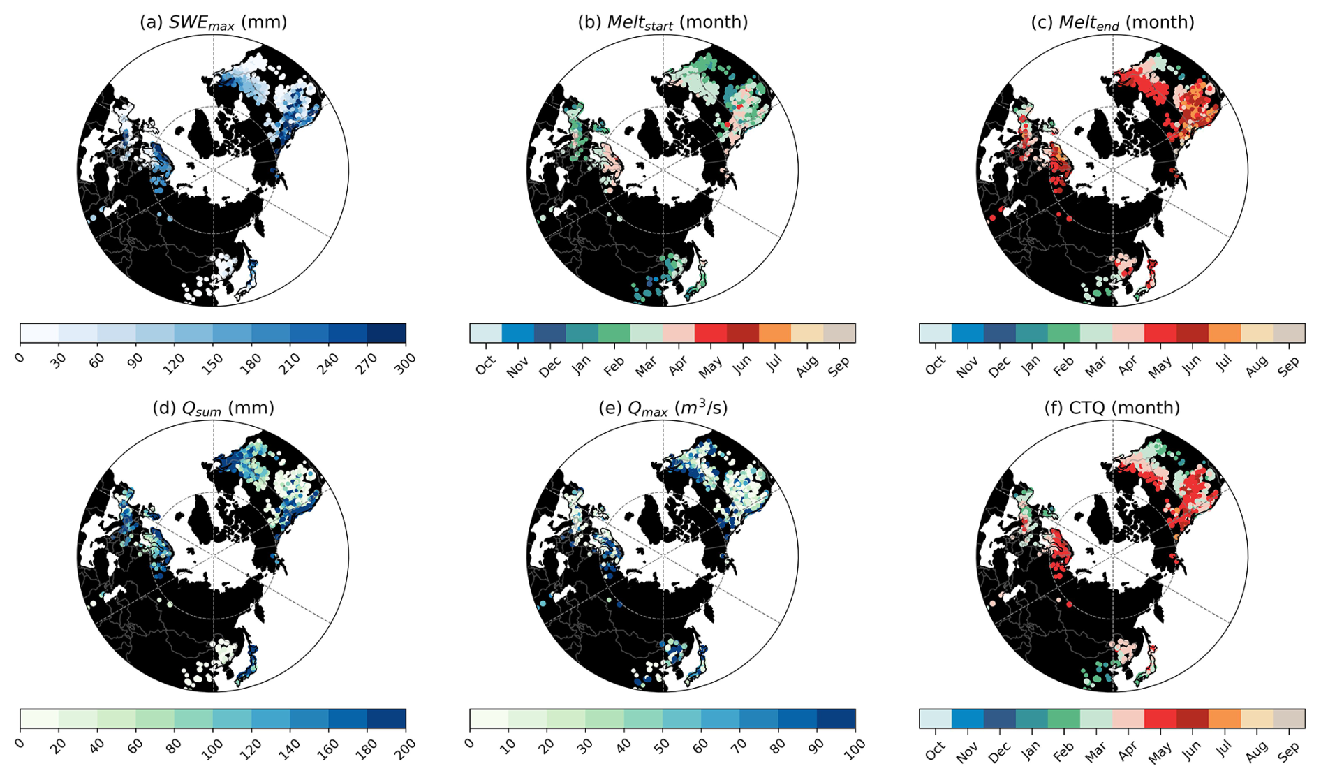
Figure 2 The spatial pattern of snow and runoff characteristics. (a) shows maximum snow water equivalent, (b) and (c) show the start and end timing of snowmelt. (d)–(e) present total runoff (Q_sum), peak flow (Q_max) and centroid timing of runoff (CTQ) during the snowmelt period, respectively. Melt_start, Melt_end, and CTQ are shown as the months instead of 'Day of Water Year' (DOY) for better interpretation of the results.

2.2.3 Quantifying the complexity of basins

To quantify the impact of land surface complexity on SMR simulation, it is essential to first identify the primary factors that may challenge model performance. Based on existing literature (Li et al., 2022; Poulter et al., 2011; Torres-Rojas et al., 2022; Harper et al., 2023), we focus on two key dimensions of basin complexity: topography and vegetation. Topographic complexity affects SMR simulation through several mechanisms. Mean elevation influences temperature, precipitation phase, snow accumulation, sublimation, and snow–radiation interactions, whereas topographic relief introduces finer-scale variations in surface energy balance, snow redistribution, melt timing, and runoff generation. Vegetation complexity also affects SMR-related processes through canopy density and vegetation composition. Higher canopy density can enhance snow interception, sublimation, and canopy shading, while greater diversity in plant functional types increases landscape heterogeneity in energy exchange and hydrological responses (Li et al., 2022).

Correspondingly, we selected four metrics to represent these two major dimensions of basin complexity: mean elevation (denoted as DEM), topographic variability (denoted as DEMstd), mean leaf area index (denoted as LAI), and the entropy of plant functional type (denoted as PFTh). Specifically, DEM represents the mean elevation background and associated climatic controls, while DEMstd reflects within-basin terrain heterogeneity. LAI represents vegetation density and its effects on canopy–snow interactions, whereas PFTh describes vegetation-type diversity and the heterogeneity of vegetation-related hydrological and energy-exchange processes. Together, these metrics form a four-dimensional vector describing the overall topographic and vegetation complexity of a basin, where higher values generally denote more challenging conditions for SMR simulation.

To synthesize this multi-faceted complexity, we introduced a basin Complexity Index (CI) by summing the normalized values of these four metrics (Eq. 4). This index is designed to provide a simple and physically interpretable representation of the major topographic and vegetation controls on SMR simulation difficulty:

$$\begin{array}{}\text{(4)}& \mathrm{CI}={\mathrm{DEM}}_{\mathrm{norm}}+{\mathrm{DEMstd}}_{\mathrm{norm}}+{\mathrm{LAI}}_{\mathrm{norm}}+{\mathrm{PFTh}}_{\mathrm{norm}}.\end{array}$$

We acknowledge that these four components may not contribute equally to hydrological complexity and that dependencies may exist among them. Therefore, we further examined the correlations among the CI components (Appendix Fig. A1). This additional analysis shows that, although some dependence exists among the components, especially between DEM and DEMstd, the four variables capture complementary topographic and vegetation controls on SMR simulation.

To further clarify the physical meaning of CI, we examined the spatial distributions of both the individual components and the integrated CI (Fig. 3). The four components show distinct but complementary spatial patterns, indicating that basin complexity is jointly shaped by elevation background, topographic variability, vegetation density, and vegetation-type heterogeneity. The integrated CI highlights several regions with relatively high basin complexity, including the western United States, western Europe, Japan, and northeastern China, where complex terrain and/or vegetation conditions may pose greater challenges for SMR simulation. These spatial patterns support the use of CI as a synthetic descriptor of basin complexity and provide a basis for interpreting subsequent model-performance changes along the CI gradient.

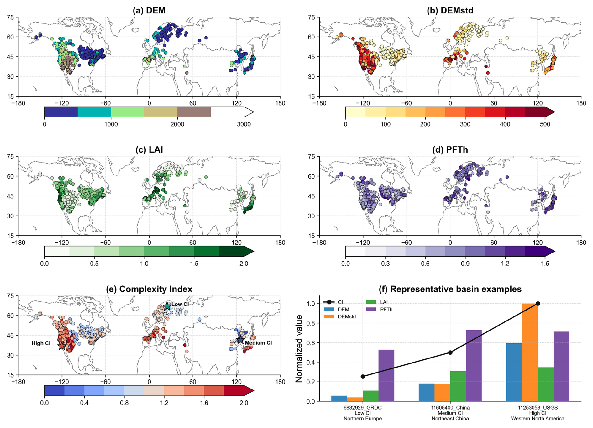
Figure 3 Spatial distribution of basin complexity components and representative examples of the integrated Complexity Index. Panels show (a) DEM, (b) DEMstd, (c) LAI, (d) PFTh, and (e) the integrated Complexity Index (CI) across the study basins. The three starred basins in panel (e) are representative examples of Low CI, Medium CI, and High CI conditions. Panel (f) compares the normalized values of DEM, DEMstd, LAI, PFTh, and CI for these three representative basins.

Consequently, we consider a model to be robust in representing SMR processes if it not only performs well in basins with low basin complexity, but also maintains its accuracy as basin complexity increases. Our analysis therefore examines model performance against each complexity factor individually, and then assesses model performance along the integrated CI gradient.

2.2.4 Measuring robustness of models

As described above, a robust model should accurately simulate SMR across diverse land-surface conditions. In this study, robustness is assessed by examining how model bias changes along the basin complexity gradient. Specifically, we developed a Robustness Index (RI) from two complementary perspectives: (1) the overall magnitude of model bias across all basin-complexity levels, hereafter referred to as performance stability; and (2) the rate at which model bias changes as basin complexity increases, hereafter referred to as adaptability.

Before calculating RI, all basins were ranked according to their integrated CI and divided into ten equal-sized groups along the CI gradient. Each group therefore represents one basin complexity level, from the least complex to the most complex basins. For each group, the representative CI value was defined as the median CI of all basins within that group, and the model bias was summarized using the median bias across basins in the same group. This grouping strategy reduces the influence of uneven basin distributions along the CI gradient and allows model performance to be evaluated consistently across different environmental complexity levels.

First, to quantify the overall bias magnitude, we calculated the Stratified Mean Absolute Bias (SMAB). SMAB represents the average absolute bias across the full CI gradient and is used here as a measure of performance stability. Compared with a direct average over all basins, this stratified calculation avoids potential distortion caused by uneven basin distributions along the complexity gradient and provides a more balanced estimate of model performance across different basin complexity levels. SMAB is calculated as follows (Eq. 5):

$$\begin{array}{}\text{(5)}& \mathrm{SMAB}={\displaystyle \frac{\mathrm{1}}{{\mathrm{CI}}_n}}\sum _{i=\mathrm{1}}^{n-\mathrm{1}}{\displaystyle \frac{\left|{\mathrm{Bias}}_i\right|+\left|{\mathrm{Bias}}_{i+\mathrm{1}}\right|}{\mathrm{2}}}\left({\mathrm{CI}}_{i+\mathrm{1}}-{\mathrm{CI}}_i\right)\end{array}$$

where i denotes the index of the complexity groups, ranging from 1 to n−1, Bias_i represents the median model bias within the ith complexity group, and CI_i indicates the representative CI value of that group.

Second, to quantify the sensitivity of model performance to increasing basin complexity, we regressed the absolute bias against CI using simple linear regression. The regression slope S was adopted as a measure of adaptability. A larger positive slope indicates that model bias increases more rapidly with basin complexity, implying stronger performance degradation and weaker adaptability under complex land-surface conditions. The regression is expressed as follows (Eq. 6):

$$\begin{array}{}\text{(6)}& \left|{\mathrm{Bias}}_i\right|=S\times {\mathrm{CI}}_i+b\end{array}$$

where S is the slope of the absolute bias along the CI gradient, and b is the intercept.

For comparison across all models, both SMAB and S were normalized to a [0,1] scale. The two normalized metrics describe complementary aspects of model robustness. Specifically, SMAB_norm reflects the overall magnitude of model bias across the full basin complexity gradient and therefore represents performance stability. S_norm reflects the rate of bias increase with basin complexity and therefore represents adaptability to complex basin conditions. A robust model should have both low SMAB_norm and low S_norm, indicating low overall bias and weak performance degradation as basin complexity increases.

Together, these two components form a two-dimensional metric space, represented by the vector (SMAB_norm,S_norm). In this space, the origin point (0,0) represents an ideal model with zero average bias and no degradation trend along the CI gradient. Following previous studies that use distance-based approaches to integrate multiple performance dimensions (Kay et al., 2007; Oudin et al., 2010; Hu et al., 2022), we adopted the Euclidean distance from this ideal point to define RI. A larger distance indicates a greater deviation from the ideal condition and therefore lower robustness. The final RI is calculated as one minus this distance (Eq. 7):

$$\begin{array}{}\text{(7)}& \mathrm{RI}=\mathrm{1}-\sqrt{{\mathrm{SMAB}}_{\mathrm{norm}}^{\mathrm{2}}+S_{\mathrm{norm}}^{\mathrm{2}}}\end{array}$$

A higher RI value indicates that a model is closer to the ideal origin point, reflecting both lower overall bias and stronger adaptability to increasing basin complexity. In this formulation, models with large overall bias are penalized through SMAB_norm, whereas models whose errors increase rapidly along the CI gradient are penalized through S_norm. Therefore, RI provides an integrated measure of model robustness by jointly accounting for performance stability and adaptability. We note that RI is used here primarily as a relative robustness metric for inter-model comparison, rather than as an absolute measure of model performance.

To clarify the interpretation of RI, we added a conceptual illustration in the Appendix Fig. A2. The schematic shows that a model with low SMAB and low slope corresponds to high robustness, whereas a model with either large overall bias or strong bias increase along the CI gradient receives a lower RI. Meanwhile, to further examine whether the RI-based model ranking is strongly affected by the specific aggregation method, we conducted a set of sensitivity experiments using alternative RI formulations (Table A1 and Fig. A3). These experiments included weighted Euclidean-distance formulations and weighted linear formulations with different relative weights assigned to SMAB_norm and S_norm. The results show that most models exhibit limited changes in both RI magnitude and relative ranking across the sensitivity experiments. In particular, models with consistently high or low robustness remain generally stable, indicating that the identification of robust and non-robust models is not strongly affected by the specific weighting scheme. Based on these sensitivity results, and considering that Euclidean-distance-based metrics have been widely used in previous studies to integrate multiple performance dimensions (Kay et al., 2007; Oudin et al., 2010; Hu et al., 2022), we retained the equal-weight Euclidean-distance formulation as the baseline RI calculation. This formulation provides a simple and physically interpretable way to jointly represent performance stability and adaptability, while avoiding the need to impose subjective preference on either component. Therefore, RI is used here as a relative and integrated measure of model robustness for inter-model comparison.

3 Results

3.1 The performance of 15 models and datasets

We first present the distribution of model biases in three key SMR characteristics (Q_sum, Q_max, and CTQ) across multiple models and datasets (Fig. 4). It is evident from Fig. 4 that most models and datasets exhibit notable biases in simulating SMR characteristics. Specifically, 10 out of 15 tend to underestimate Q_sum and Q_max, while CTQ is generally predicted earlier than observed (14 out of 15). Although a few models perform consistently well, considerable variability exists across metrics. The following sections provide a detailed assessment of Q_sum, Q_max, and CTQ, respectively. Fig. 4a shows that the highest accuracy of Q_sum is achieved by discharge datasets (i.e., GRDR and GRADES), followed by GHMs (blue bars) and LSMs (yellow bars). GRDR and GRADES have 42.4 % and 40.1 % of basins, respectively, that lie within the ±20 % threshold, and with a median bias of −10.3 % and 0.7 %. Among models, WATERGAP2-2E performs the best (30.1 %, −1.8 %), while VIC, MATSIRO, and MIROC-INTEG-LAND show the poorest performance, each with median biases exceeding −50 %. These results highlight persistent underestimation in many physically based models, while underscoring the advantage of observation-constrained datasets. Details of each model's performance are shown in Appendix Fig. A4.

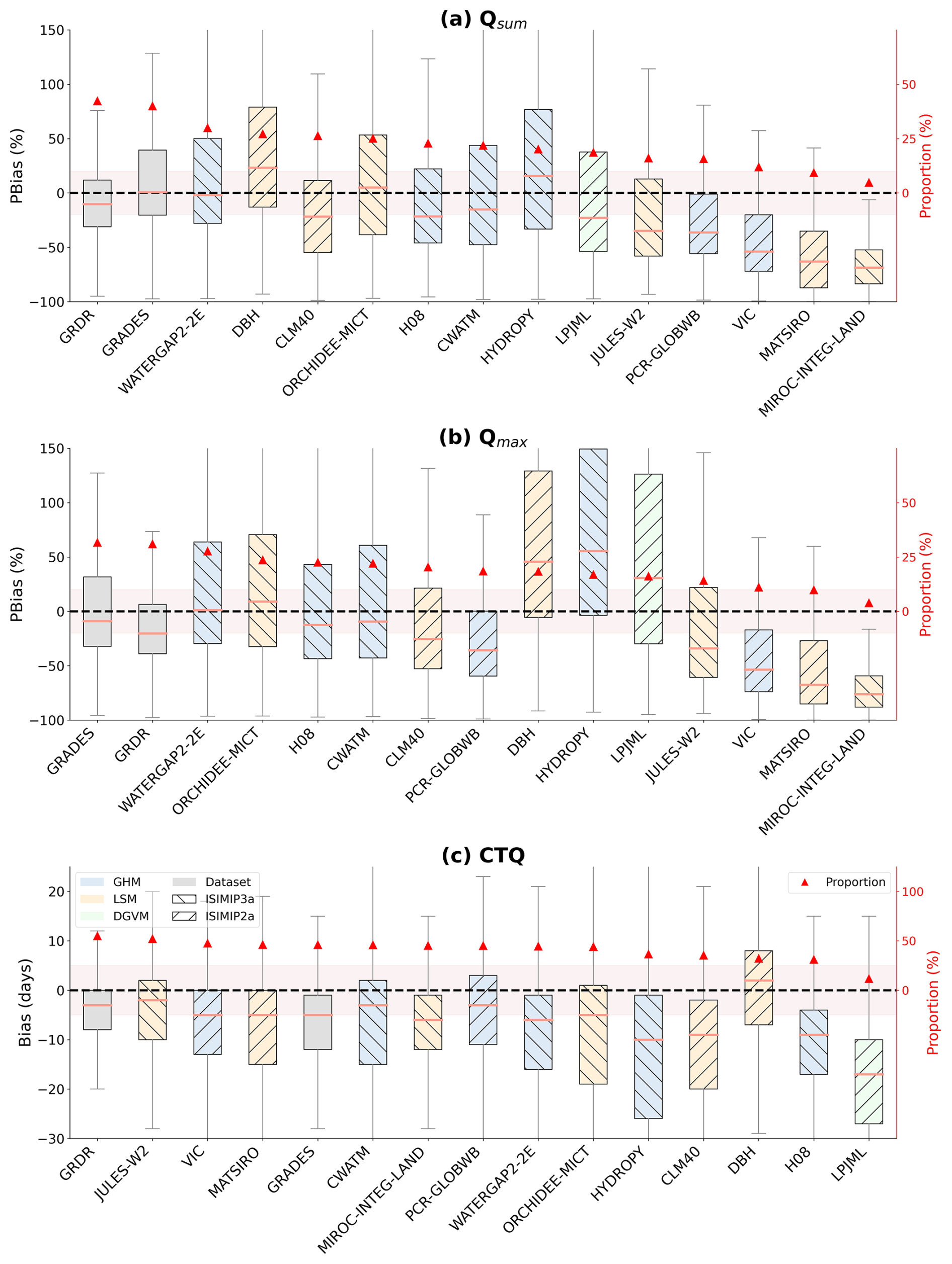
Figure 4 Evaluation of key SMR characteristics (averaged over 1979–2019) simulated by 15 models/datasets across 1455 basins. (a)–(c) present total runoff (Q_sum), peak flow (Q_max), and centroid timing of runoff (CTQ) of the SMR, respectively. The black dashed line denotes zero bias, and the red shading denotes the acceptable ranges (±20 % for Q_sum and Q_max, ±5 d for CTQ). Model rankings are determined by the proportion of basins falling within these ranges (e.g., red triangle). Model categories (e.g., GHMs, LSMs, DGVM, and Datasets) and ISIMIP phases are distinguished by background color and hatch patterns.

Figure 4b presents results for Q_max, which largely resemble Q_sum but exhibit generally worse performance. The same three models (i.e., GRADES, GRDR, and WATERGAP2-2E) again lead in performance (with 31.8 %, 31.1 %, and 27.8 % of basins, respectively, lying within the acceptable range). The weakest performers remain unchanged (VIC, MATSIRO, MIROC-INTEG-LAND), but with lower proportions in the acceptable range (11.2 %, 10.0 %, and 4.0 %). HYDROPY achieves 20.3 % basin with bias within ±20 % for Q_sum (median bias: 23.3 %), but only 17.0 % for Q_max (55.5 %). On average, models tend to simulate Q_sum with higher fidelity than Q_max (22.2 % vs. 19.3 %), reflecting greater challenges in capturing peak flows, which are more sensitive to melt rate and timing.

Model performance for CTQ (Fig. 4c) displays a distinct pattern. GRDR remains the best, with 55.2 % of basins within ±5 d and a median bias of −3 d. However, rankings among models diverge substantially from those for Q_sum and Q_max. Notably, VIC, MATSIRO, and JULES-W2 – previously among the least accurate for Q_sum and Q_max – rank among the top performers for CTQ. Conversely, models such as DBH, which ranked fourth for Q_sum, perform poorly for CTQ. These contrasts reflect fundamental differences in how models represent the timing versus magnitude of snowmelt, and emphasize the importance of snowpack energy balance and melt onset processes in simulating runoff timing.

In addition, we compared the performance of different model categories and ISIMIP phase (Fig. 5). The results show that GRDR and GRADES consistently outperform models, underscoring the importance of observational constraints. Among models, GHMs generally outperform LSMs in simulating Q_sum and Q_max, whereas LSMs show better performance for CTQ (Fig. 5e).

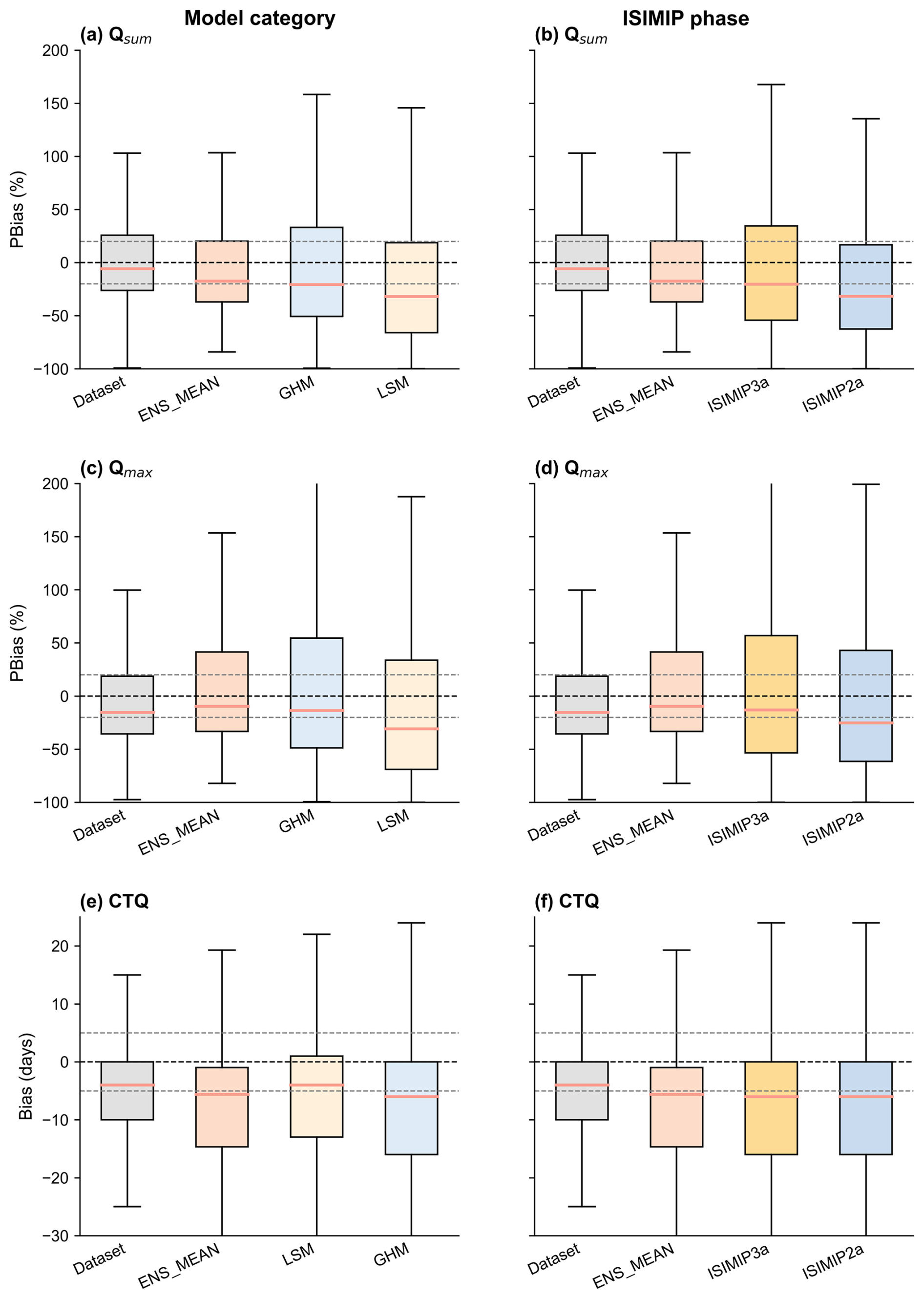
Figure 5 Evaluation of simulated runoff over 1979–2019 across 1455 catchments grouped by model category and ISIMIP phase. Panels (a), (c), (e) show the bias distributions grouped by model category, including global hydrological models (GHMs), land surface models (LSMs), observation-constrained runoff datasets (Dataset), and the ensemble mean of all individual models (ENS_MEAN). Panels (b), (d), (f) show the corresponding results grouped by ISIMIP phase. Rows represent the three snowmelt runoff characteristics: total runoff (Q_sum; a–b), peak flow (Q_max; c–d), and centroid timing of runoff (CTQ; e–f). The black dashed line indicates zero bias, and the gray dashed lines denote the acceptable ranges (±20 % for Q_sum and Q_max, and ±5 d for CTQ). Groups are ordered according to the proportion of basins falling within these acceptable ranges, with category-level rankings calculated from the average performance of individual models within each group.

This contrast likely reflects the distinct physical controls underlying the three runoff characteristics. Q_sum and Q_max are more closely related to runoff magnitude and water-balance closure during the snowmelt period, and therefore may benefit from runoff-generation parameterizations and streamflow-oriented calibration strategies that are commonly emphasized in GHMs. In contrast, CTQ mainly reflects the timing and rate of snowmelt release, which are more directly controlled by energy-exchange processes and snowpack evolution. This interpretation is also consistent with the process complexity analysis in Part 2 (Lei et al., 2026), which shows that LSMs generally include more detailed energy-related process representations, such as energy-balance snowmelt schemes, canopy radiative transfer parameterizations. These features are particularly important for capturing melt timing and may partly explain why LSMs show relative advantages in CTQ simulation. Notably, two of the three models for CTQ are LSMs (Fig. 4c), further suggesting that physically based energy-related process representations can improve the simulation of runoff timing. However, the differences between GHMs and LSMs should not be attributed solely to model category or process representation. Calibration status, forcing datasets, model resolution, and implementation strategies may also contribute to the observed patterns. For example, several GHMs in our ensemble have explicit calibration information, whereas most LSMs are grouped as uncalibrated models, which may partly contribute to the stronger GHM performance for Q_sum and Q_max. In addition, models from ISIMIP3a outperform those from ISIMIP2a (Fig. 5). This improvement may reflect a combination of updated model structures, differences in forcing datasets, and model-specific calibration or implementation strategies, rather than model generation alone. Therefore, the category-level differences reported here should be interpreted as the combined effect of runoff-characteristic sensitivities, process representation, calibration status, and forcing data differences.

We further evaluate the spatial performance of the models (Fig. 6), which shows the overall biases, inter-model differences, and the best-performing model at each site. Figure 6a–c highlights the spatial patterns of ensemble mean simulation bias. Widespread underestimation and earlier runoff timing are observed across several regions, including the western coastal and mountainous areas of the United States, western and northern Europe, northeastern China, and Japan. In more than 50 % of the basins within these regions, Q_sum and Q_max exhibit negative biases ranging from 0 % to −60 %, while CTQ occurs up to 15 d earlier than observed. Meanwhile, significant overestimations are found in the central United States and northern China. Across all basins, the proportion meeting the predefined performance thresholds, i.e., bias within ±20 % for Q_sum and Q_max, and within −5 d for CTQ, is 27.9 %, 29.4 %, and 45.0 %, respectively. These basins are mainly located along the eastern coast of the United States. Detailed spatial maps of each model's performance are shown in Appendix Figs. A5–A7.

We also assess inter-model consistency in Fig. 6d–f, which shows the largest inter-model discrepancies occur in the central United States, northern Europe, and northeastern China, where CV for Q_sum and Q_max exceeds 0.8 and the CTQ range exceeds 30 d. Basins with relatively low variability, defined as CV < 0.4 or CTQ range < 20 d, occupy 20.7 %, 15.2 %, and 24.6 % of all basins for Q_sum, Q_max, and CTQ, respectively. These basins are primarily located in mid- to low-latitude regions of the United States and western Europe.

Figure 6g–i identifies the best-performing model in each basin, with the top two models highlighted in pie charts to examine whether any model demonstrates broad applicability. The results suggest that, no single model or dataset consistently outperforms others across all basins. For the SMR magnitude (i.e., Q_sum and Q_max), GRDR and GRADES emerge as the best ones, each being the best-performing model in over 10 % of basins. The remaining 70 % of basins are distributed among several other models, each contributing approximately 5 % on average. For the SMR timing (i.e., CTQ), DBH and PCR-GLOBWB are the most frequently selected, accounting for 14.1 % and 13.3 % of basins, respectively. These findings underscore the inconsistency in optimal model selection across different runoff characteristics.

Overall, basins exhibiting larger simulation biases tend to also display greater inter-model variability, indicating the persistent SMR challenges within these regions. This may be attributed to: (1) the complex land conditions, which makes it difficult for models to accurately represent relevant physical processes, and (2) differing model complexities, where simpler and more complex models diverge more significantly under such land conditions. These jointly determine the increased biases and reduced consistency there. Furthermore, model performance varies across basins–strong performance in one basin does not guarantee similar performance elsewhere. This highlights that no single model is universally applicable, and that model selection should consider both complexity of the basin and the model's ability to represent key physical processes.

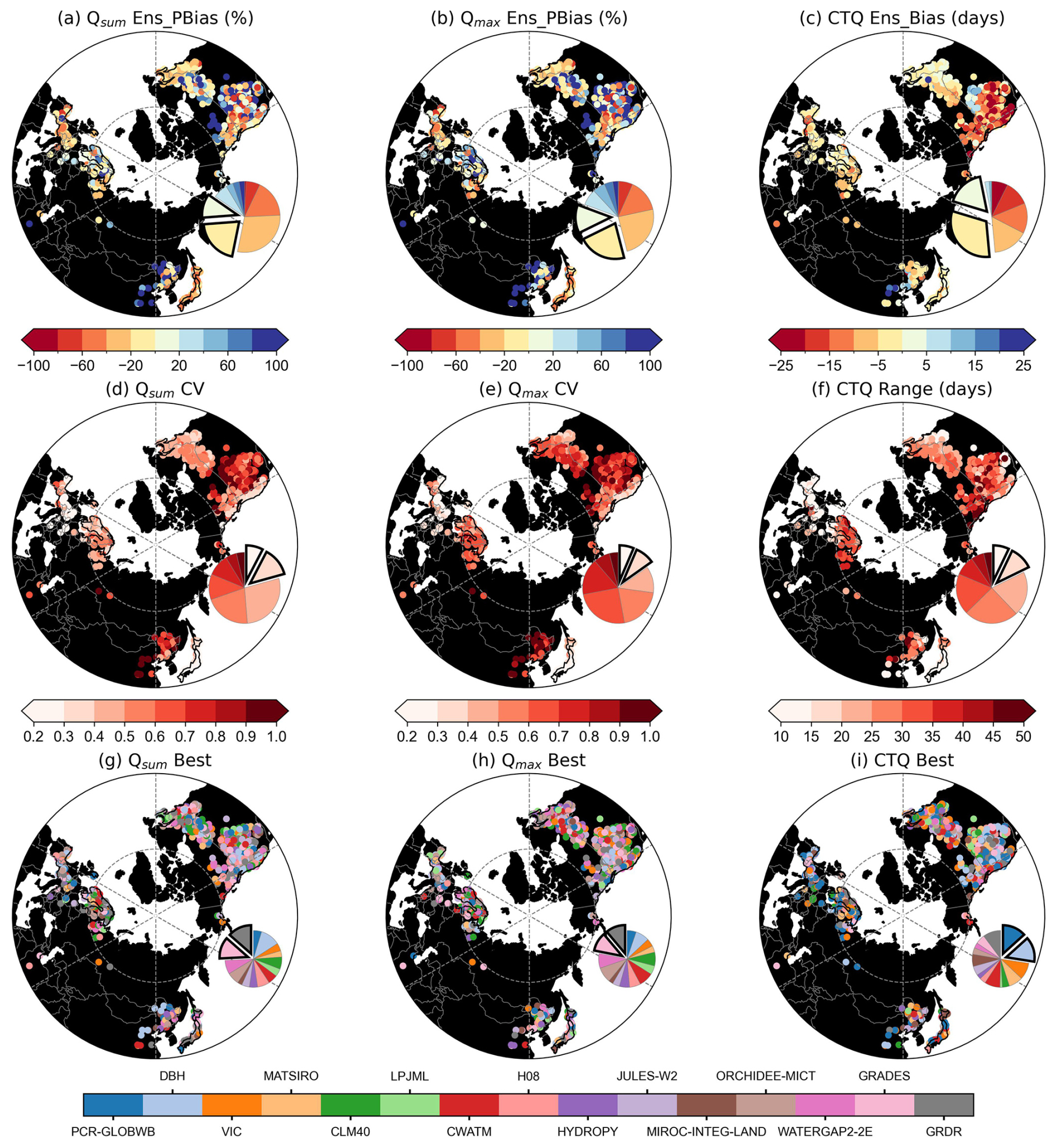
Figure 6 Bias, variability, and the best model for simulated SMR characteristics across different basins. (a)–(c) show the percent bias of Q_sum (%), percent bias of Q_max (%), and bias of CTQ (days), respectively, in the simulated SMR. (d)–(f) show inter-model variability represented by the coefficient of variation (CV) for Q_sum and Q_max, and inter-model range of CTQ (days). (g)–(i) show the model with the smallest bias in each basin for Q_sum, Q_max, and CTQ, respectively. The pie charts provide a summary of these patterns, with bold black outlines highlighting the proportion within ±20 % bias in (a)–(c), the two lowest variability levels in (d)–(f), and the top two models with the highest proportions in (g)–(i).

3.2 Impacts of land surface complexity on model performance

To understand how land surface complexity influences model performance, we next analyze the results to identify general patterns, dissect the effects of different complexity sources, and compare the behaviors of models with varying structures. The most pervasive pattern is that model performance deteriorates as basin complexity increases (Fig. 7a–c). For the majority of models, biases in simulating Q_sum, Q_max, and CTQ grow as the land surface becomes more complex, confirming the hypothesis that many models have a limited ability to capture intricate land surface processes in such environments. Among the three characteristics, the bias in CTQ increases most markedly with basin complexity, followed by Q_max and Q_sum. Moreover, this fragility in CTQ is particularly evident beyond a certain complexity threshold (Fig. 7c), where performance deteriorates sharply for nearly all models, suggesting a potential breakdown in their ability to handle compounded, non-linear landscape effects. For Q_sum and Q_max, two distinct groups of models can be identified: those with consistently low bias (e.g., GRDR and GRADES) and those with consistently high bias (e.g., VIC). Notably, GRADES is based on VIC runoff simulations constrained by observations, while GRDR further assimilates remotely sensed river width information. The result provides an initial assessment of the gain from data assimilation as a strategy for correcting inherent model. Detailed relationships between each factor and the model performance can be found in the Appendix Figs. A8–A10.

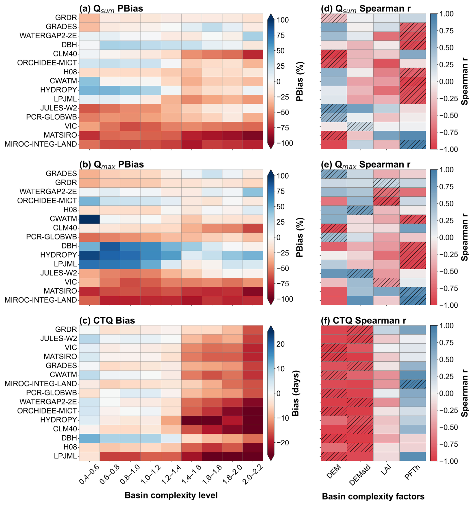
Figure 7 Influence of basin complexity on model simulations of key runoff characteristics. (a)–(c) show the variation in model performance as basin complexity increases, and (d)–(f) represent the Spearman correlation between model performance and individual basin complexity factors. A positive correlation indicates that model bias increases with increasing basin complexity, whereas a negative correlation indicates that model bias decreases as basin complexity increases. Shading indicates the basin complexity factor with the highest absolute Spearman correlation among the four factors.

A deep dive into specific model comparisons offers interesting insights into how different model structures handle complexity. A noteworthy and counterintuitive observation is the improved performance of certain physically complex models in more challenging land surface. For example, models like JULES-W2 and PCR-GLOBWB exhibit an unexpected trend where their simulation bias for Q_sum decreases as basin complexity increases (Fig. 7a). This suggests that the advanced process representations within these models, which might be less critical in simple, homogeneous basins, become advantageous in complex terrain. For instance, JULES-W2’s sophisticated schemes for canopy interception, sublimation, and radiation transfer are explicitly designed to handle the fine-scale variability introduced by complex topography conditions (Fig. 7d). However, we would like to note that while the result points to the potential of sophisticated physics to enhance model robustness, further diagnostic analysis is essential to confirm whether this improved performance reflects a genuinely better process representation.

The analysis also reveals significant structural trade-offs in how different models respond to complexity, particularly when comparing the simulation of Q_sum and Q_max. This is exemplified by the opposing responses of DBH and LPJML: in complex basins, DBH improves its Q_max (Fig. 7b) simulation while degrading its Q_sum (Fig. 7a) simulation, whereas LPJML exhibits the inverse pattern. These contrasting responses may reflect differences in how the two models simulate runoff generation for different flow characteristics. A model like DBH may have a structure that better represents the fast, event-based runoff pathways critical for capturing flood peaks, while LPJML might be better structured to simulate the slow, integrated processes that determine the long-term water balance. These findings imply that no single model structure currently excels at both functions in complex environments, highlighting the need to select models based on the specific scientific question at hand.

When the overall complexity is decomposed into its constituent components, a clear hierarchy of influence emerges (Fig. 7d–f). The bias in simulated Q_sum is primarily driven by variations in DEM and PFTh (Fig. 7d). This likely reflects the strong link between DEM and processes such as rainfall–snowfall partitioning and sublimation, while PFTh affects the accuracy of interception representation. These processes jointly determine the accuracy of Q_sum simulation. In comparison, the bias in simulated Q_max is more strongly influenced by vegetation cover (e.g., LAI) and vegetation type diversity (e.g., PFTh) (Fig. 7e). Both LAI and PFTh affect the amount of energy and water reaching the ground surface; during the snowmelt period, the extent to which liquid precipitation interception is properly represented can substantially impact Q_max. The timing metric CTQ is mainly controlled by topographic factors (Fig. 7f), particularly DEM and its variability (DEMstd), likely because CTQ is more sensitive to energy-related processes, and both DEM and DEMstd are key determinants of surface energy balance. Overall, topography remains the dominant driver of model bias, underscoring its critical role in shaping runoff dynamics, while vegetation exerts a comparatively secondary influence. Their combined interactions ultimately govern the magnitude and structure of the overall model bias.

3.3 Assessment of Model Robustness

We further evaluate the aforementioned model's robustness by analyzing performance across the defined complexity groups (Fig. 8). By focusing on two aspects of our robustness metric, we aim to identify significant performance differences among the models or model groups and explore the underlying reasons for these variations. Models with lower stability and lower adaptability are considered higher robust in reproducing runoff characteristics (Fig. 8a).

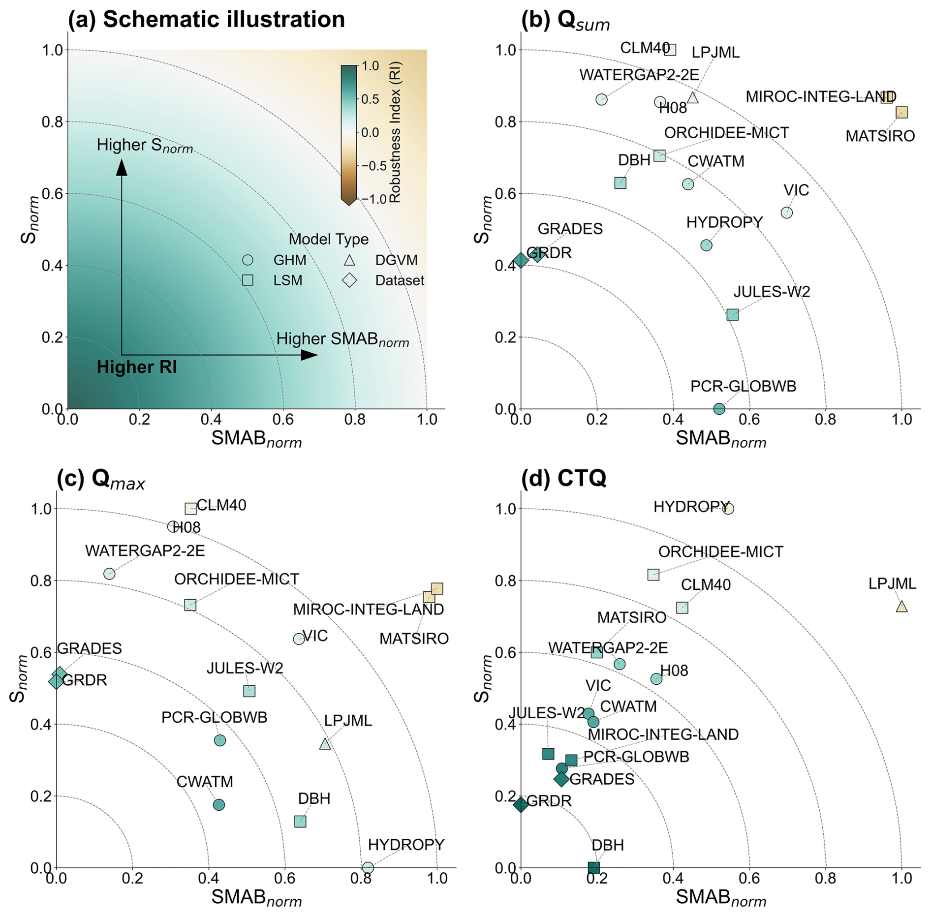
Figure 8 Assessment of model robustness in key SMR characteristics. (a) Schematic illustration. (b–d) Results for Q_sum, Q_max, and CTQ, respectively. Circles denote global hydrological models (GHMs), squares denote land surface models (LSMs), triangles denote dynamic global vegetation models (DGVMs), and diamonds denote data products. SMAB_norm denotes the normalized stratified mean absolute bias, and S_norm denotes the normalized regression slope of absolute bias. Detailed calculation procedures are provided in Sect. 2.2.4.

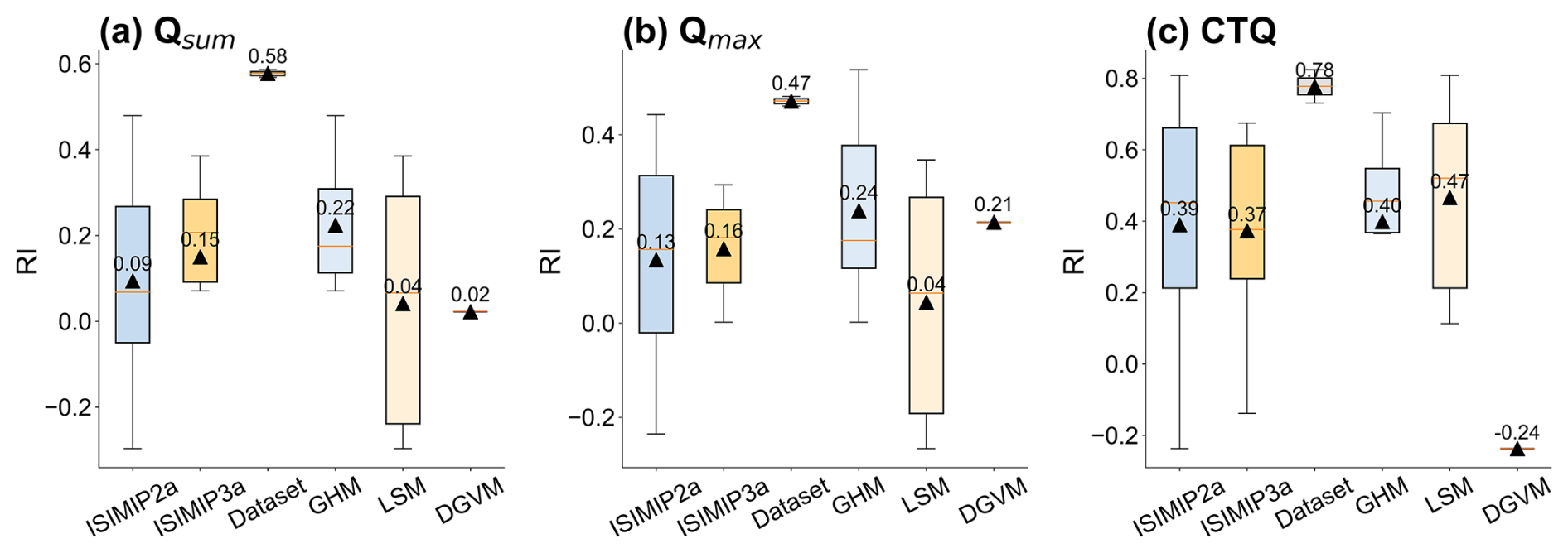
Figure 9 Assessment of model robustness in key SMR characteristics grouped by model categories and ISIMIP phase. (a)–(c) show results for Q_sum, Q_max, and CTQ, respectively. The orange line denotes the median, the black triangle indicates the mean, and the classifications of model types and ISIMIP phases follow Sect. 2.1.1.

Overall, the models with the highest robustness for Q_sum are GRDR, GRADES, and PCR-GLOBWB (Fig. 8b). These models exhibit both low average bias and minimal performance degradation as land surface complexity increases. In contrast, models like CLM40, MATSIRO, and MIROC-INTEG-LAND rank the lowest, primarily due to their large simulation biases. The robustness rankings for Q_max are generally consistent, with GRDR, GRADES again performing well (Fig. 8c). However, a key difference is that several models, such as CWATM and HYDROPY, exhibit significant improvements in simulating Q_max in more complex basins, hinting at structural differences in how they handle event-based runoff.

The results for CTQ reveal a more critical pattern (Fig. 8d). While the overall bias is comparable across many models, the performance of nearly all models degrades sharply with increasing complexity. This indicates that runoff timing is the characteristic most sensitive to the challenges posed by complex land surfaces, as indicated in Sect. 3.2. This S_norm arises largely because timing is influenced by coupled processes that are difficult to simulate accurately in complex environments. For example, topography modulates surface radiation and alters runoff convergence, while dense and diverse vegetation complicates canopy interception and energy transfer. The inability of current models to resolve these intricate interactions leads to the sharp decline in performance for accurately predicting the timing of the snowmelt.

A deep dive into the two components of the robustness score provides more insights in model behavior. For Q_sum, some models present a clear conflict between these two metrics (Fig. 8b). Models like LPJML and CLM40 may appear accurate in simple basins, but their performance degrades rapidly in more complex environments (Fig. 7a), resulting in a higher slope and consequently greater instability in performance. Conversely, although PCR-GLOBWB exhibits a relatively large overall bias, its performance improves with increasing basin complexity (Fig. 7a), thereby achieving a high robustness ranking. This seemingly counterintuitive result may reflect a trade-off inherent in physically complex models, as their sophisticated process representations provide advantages for simulating the intricate dynamics in challenging basins but may introduce unnecessary structural uncertainty in simpler environments at the same time. Such a pattern is even more pronounced for Q_max (see Fig. 8c), where a larger set of models, including DBH and HYDROPY, exhibit a low slope. This suggests their internal structures may be better suited to capturing the dynamics of peak discharge in highly complex terrain conditions.

We further aggregate the results by model group to identify systematic differences in performance (Fig. 9). Overall, ISIMIP3a outperforms ISIMIP2a in simulating Q_sum and Q_max. Moreover, observation-constrained datasets (GRADES and GRDR) exhibit the highest robustness, followed by GHMs and LSMs. These GHMs advantage is particularly pronounced for Q_sum and Q_max (Fig. 9a–b). For CTQ (Fig. 9c), however, LSMs exhibit a clear relative improvement compared with their performance for Q_sum and Q_max, with MIROC-INTEG-LAND notably rising from the lowest tier to a leading position (Fig. 8d). This improvement likely reflects the more advanced treatment of radiative transfer and surface energy balance in LSMs, which plays a greater role in capturing melt timing than in reproducing total runoff or peak flow.

4 Conclusions and Discussions

This study provides a systematic large-sample evaluation of the ability of 15 hydrological models and runoff products to capture key runoff characteristics during the snowmelt period across 1455 basins worldwide. In addition to conventional performance assessment, we use a RI to quantify how model skill changes along basin complexity gradients. This analysis complements existing model evaluation approaches by integrating established SMR characteristics with basin complexity information, thereby providing additional insights into the stability and adaptability of model performance under diverse environmental conditions. Our primary findings are summarized as follows:

• Most models exhibit systematic biases in simulating key runoff characteristics during the snowmelt period. In particular, they tend to underestimate Q_sum and Q_max while predicting CTQ too early. These biases are especially pronounced in regions such as the western United States, northern Europe, and northeastern China, where both the magnitude of deviations and the inter-model discrepancies are substantial. GRDR and GRADES generally outperform most process-based models in reproducing SMR characteristics, highlighting the value of observational constraints. Among them, GHMs generally perform better than LSMs in simulating runoff magnitude characteristics, including Q_sum and Q_max, whereas LSMs show a clear advantage over GHMs in simulating CTQ. This contrast suggests that GHMs are more effective in reproducing snowmelt runoff magnitude, while LSMs are better suited to capturing energy-controlled melt timing. The ISIMIP3a models also show consistently higher accuracy compared to ISIMIP2a, and ensemble means typically provide more robust results than individual models.

• Model biases are substantially increased under high basin complexity, with stronger underestimation of Q_sum and Q_max and earlier estimation of CTQ. The underestimation is generally more severe for Q_max than for Q_sum. Notably, model skill in simulating CTQ declines sharply as basin complexity increases, highlighting the limited capacity of current models to capture complex snow–vegetation–topography interactions under highly heterogeneous conditions. Models show divergent responses to increasing basin complexity: GRDR and GRADES remain relatively robust, some models (e.g., JULES-W2, PCR-GLOBWB) show partial adaptability, while many others exhibit increasing biases.

• By applying the newly developed robustness metric, we find that GRDR and GRADES consistently rank at the top, with PCR-GLOBWB, JULES-W2, and DBH also performing well. By contrast, CLM40, MATSIRO, and MIROC-INTEG-LAND show low robustness for Q_sum and Q_max but improve markedly in CTQ. Overall, GHMs demonstrate higher robustness in simulating runoff magnitude characteristics, particularly Q_sum and Q_max, whereas LSMs show higher robustness in simulating CTQ. This contrast likely reflects fundamental differences in model structure: GHMs are generally more effective in maintaining stable water-balance and runoff-generation performance, while LSMs benefit from more detailed energy-balance and snowpack representations that improve the robustness of melt-timing simulation under heterogeneous conditions.

These findings advance the understanding of SMR modeling under complex land surface conditions, establishing a benchmark framework for future model development. Several limitations are worthy of further discussion for future research.

• First, it is noteworthy that ISIMIP2a and ISIMIP3a exhibit differences beyond their mechanistic descriptions of the snow accumulation and snowmelt processes. These variations include differences in forcing, simulation scenarios, and whether model calibration is applied. In our data selection process, we have minimized these discrepancies to enhance direct comparisons that emphasize process differences. However, further scrutiny may be necessary to fully delineate these differences.

• Second, the evaluation metrics of models could be further improved. While this study primarily focused on biases and robustness in simulating key SMR characteristics, it did not assess the models’ capability in reproducing the temporal dynamics of SMR. Future research should therefore focus on evaluating how well models capture the temporal dynamics of SMR.

• Third, the relationship between model performance and the completeness of physical process representation requires further investigation. Current analyses are largely conducted at the level of model categories or intercomparison projects, providing only a broad perspective on the link between model structure and performance. Future work should therefore focus on developing a unified framework to quantify model process complexity, which would allow a more rigorous evaluation of how physical process differences translate into performance disparities.

Appendix A

Table A1 Sensitivity experiments used to test the robustness of the RI formulation. Formula A: $\mathrm{RI}=\mathrm{1}-\sqrt{w\cdot {\mathrm{SMAB}}_{\mathrm{norm}}^{\mathrm{2}}+(\mathrm{1}-w)\cdot S_{\mathrm{norm}}^{\mathrm{2}}}$. Formula B: $\mathrm{RI}=\mathrm{1}-\left(w\cdot {\mathrm{SMAB}}_{\mathrm{norm}}+(\mathrm{1}-w)\cdot S_{\mathrm{norm}}\right)$.

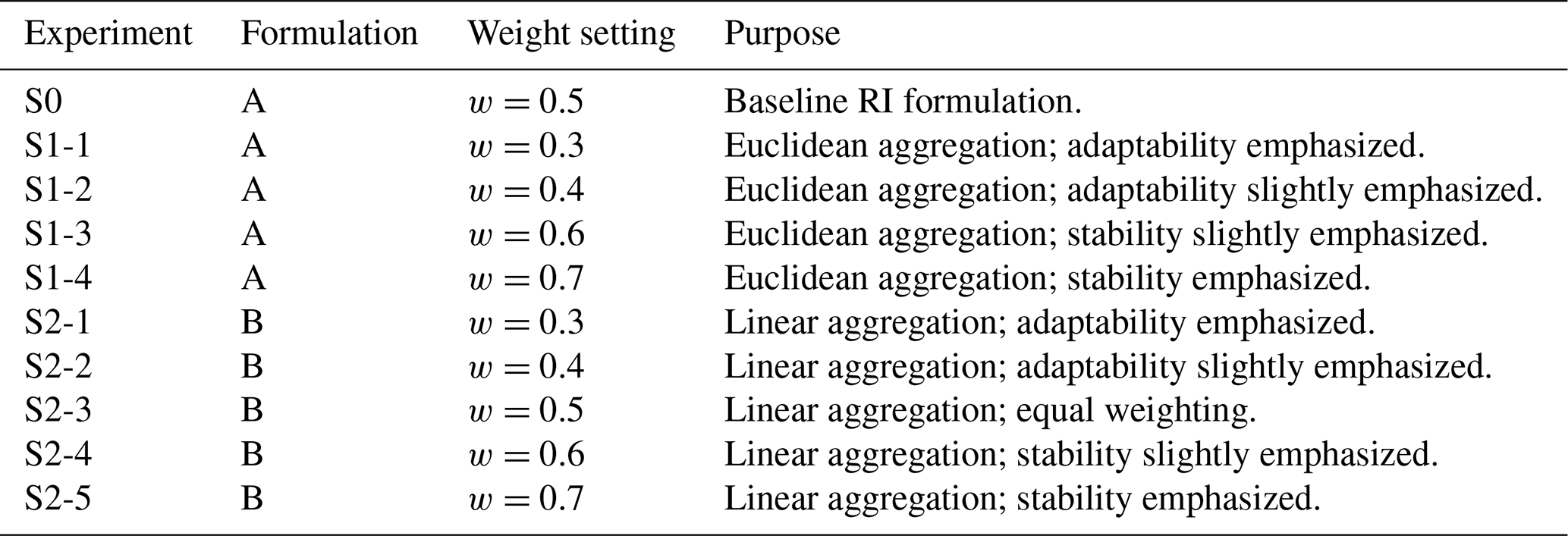
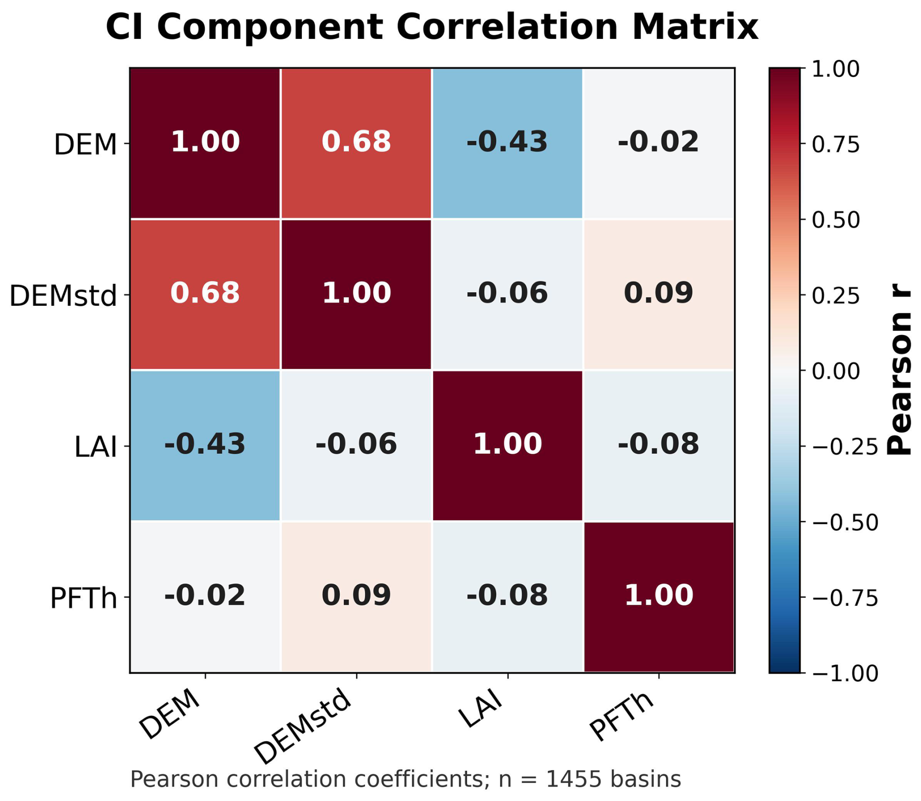
Figure A1 Pearson correlation matrix among the four components used to construct the basin complexity index. The value of each grid represents the Pearson correlation coefficients among teh DEM, DEMstd, LAI, and PFTh.

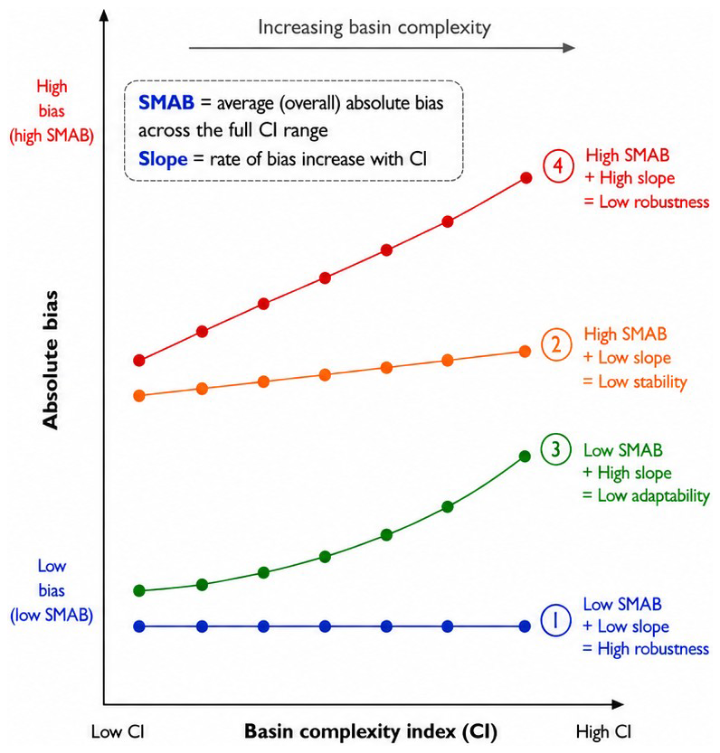
Figure A2 Conceptual illustration of the Robustness Index (RI). The stratified mean absolute bias (SMAB) represents the overall magnitude of model bias across the full basin complexity index (CI) gradient, whereas the slope represents the rate at which model bias changes with increasing CI.

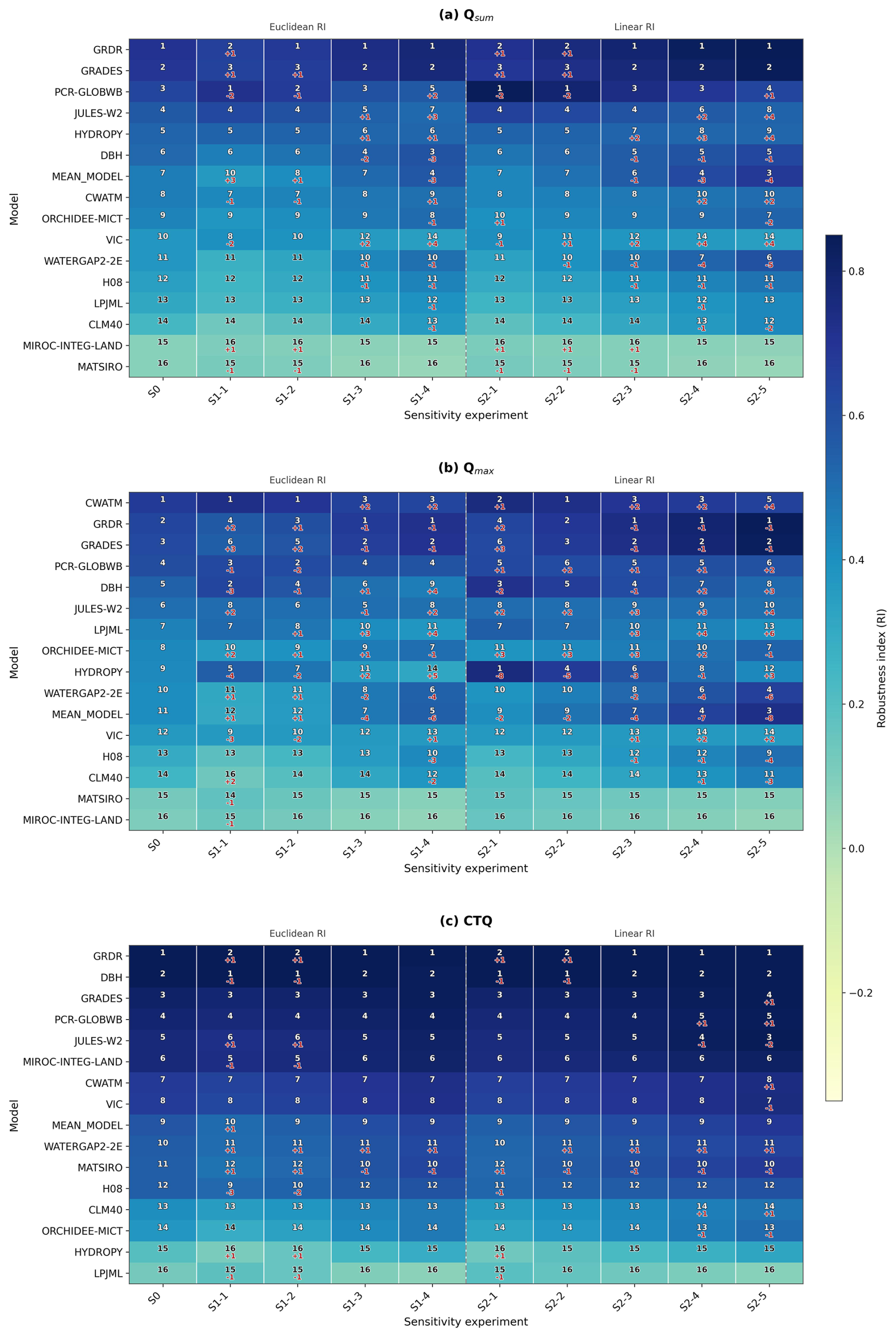
Figure A3 Sensitivity analysis of the Robustness Index (RI) formulation. Panels (a)–(c) present the sensitivity of model robustness rankings for Q_sum, Q_max, and CTQ, respectively. The sensitivity experiments include the baseline Euclidean-distance-based RI (S0), weighted Euclidean formulations (S1-1 to S1-4), and weighted linear formulations (S2-1 to S2-5). The color shading represents the RI value, and the number in each cell denotes the model rank under the corresponding experiment. Red numbers indicate rank changes relative to the baseline RI formulation.

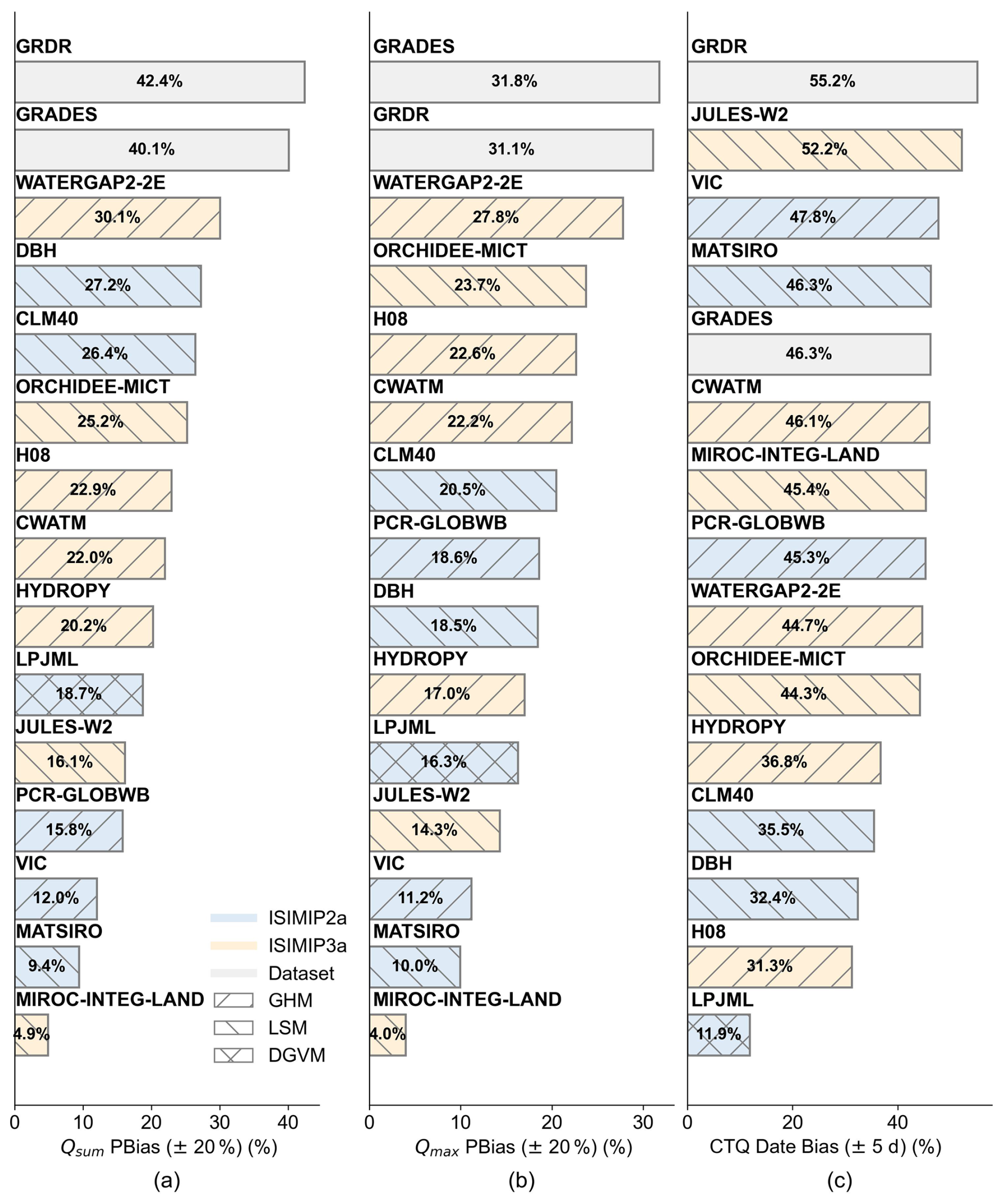
Figure A4 Percentage of gauges (%) with well-simulated snowmelt runoff indices for each model. (a) shows the percentage of gauges with good simulated CTQ (within ±5 d of the observed) as ranked by their performance. (b) and (c) show that with well-simulated Q_sum (PBias within ±20 %) and that with well-simulated Q_max (PBias within ±20 %) in the snowmelt period.

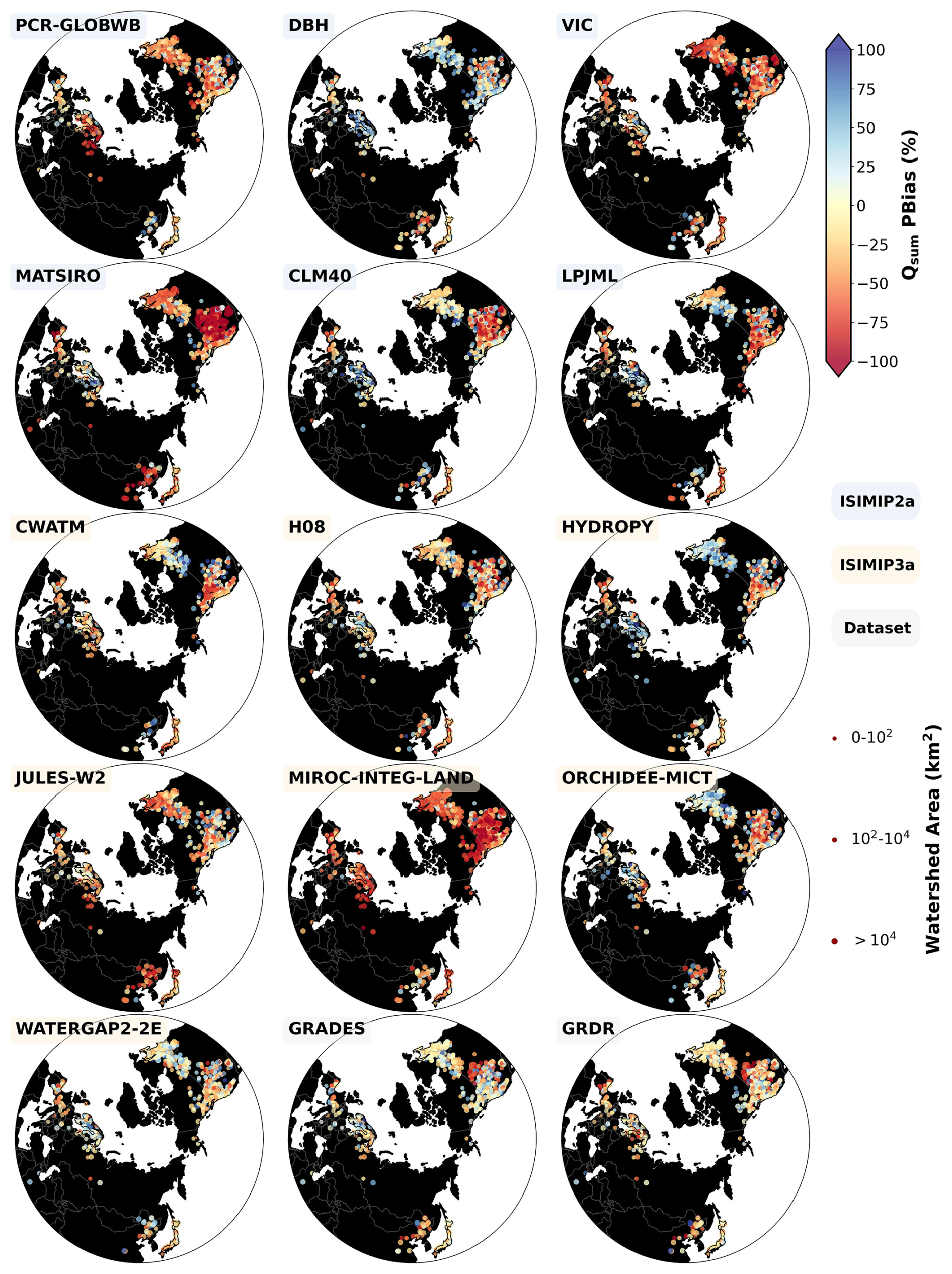
Figure A5 The percentage bias of total runoff (Q_sum) during the snowmelt period (unit: %). Colors indicate the degree of bias compared to observations: red represents underestimation, blue indicates overestimation, and yellow signifies well-matched total runoff. The point size is adjusted based on station density for better visualization and does not have physical significance. Colored boxes around model/dataset names denote three categories of data.

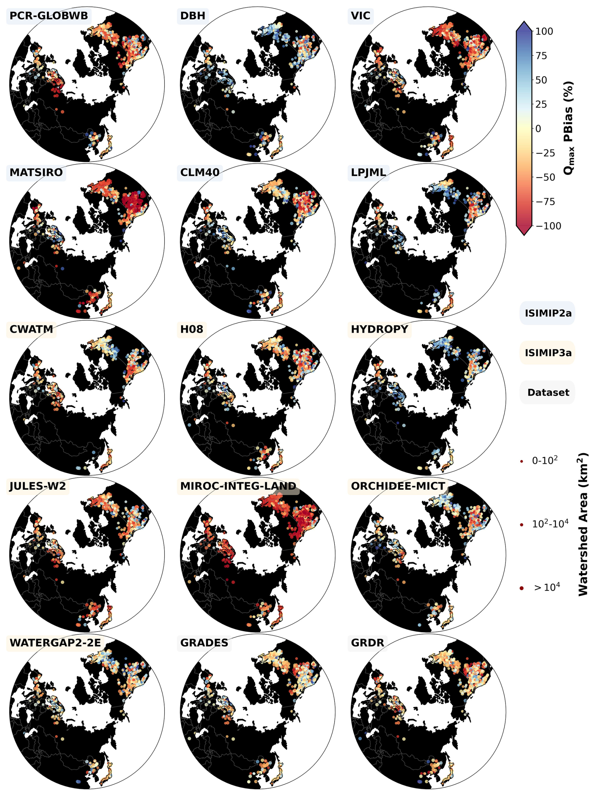
Figure A6 The percentage bias of peak flow (Q_max) during the snowmelt period (unit: %). Colors indicate the degree of bias compared to observations: red represents underestimation, blue indicates overestimation, and yellow signifies well-matched total runoff. The point size is adjusted based on station density for better visualization and does not have physical significance. Colored boxes around model/dataset names denote three categories of analysis data.

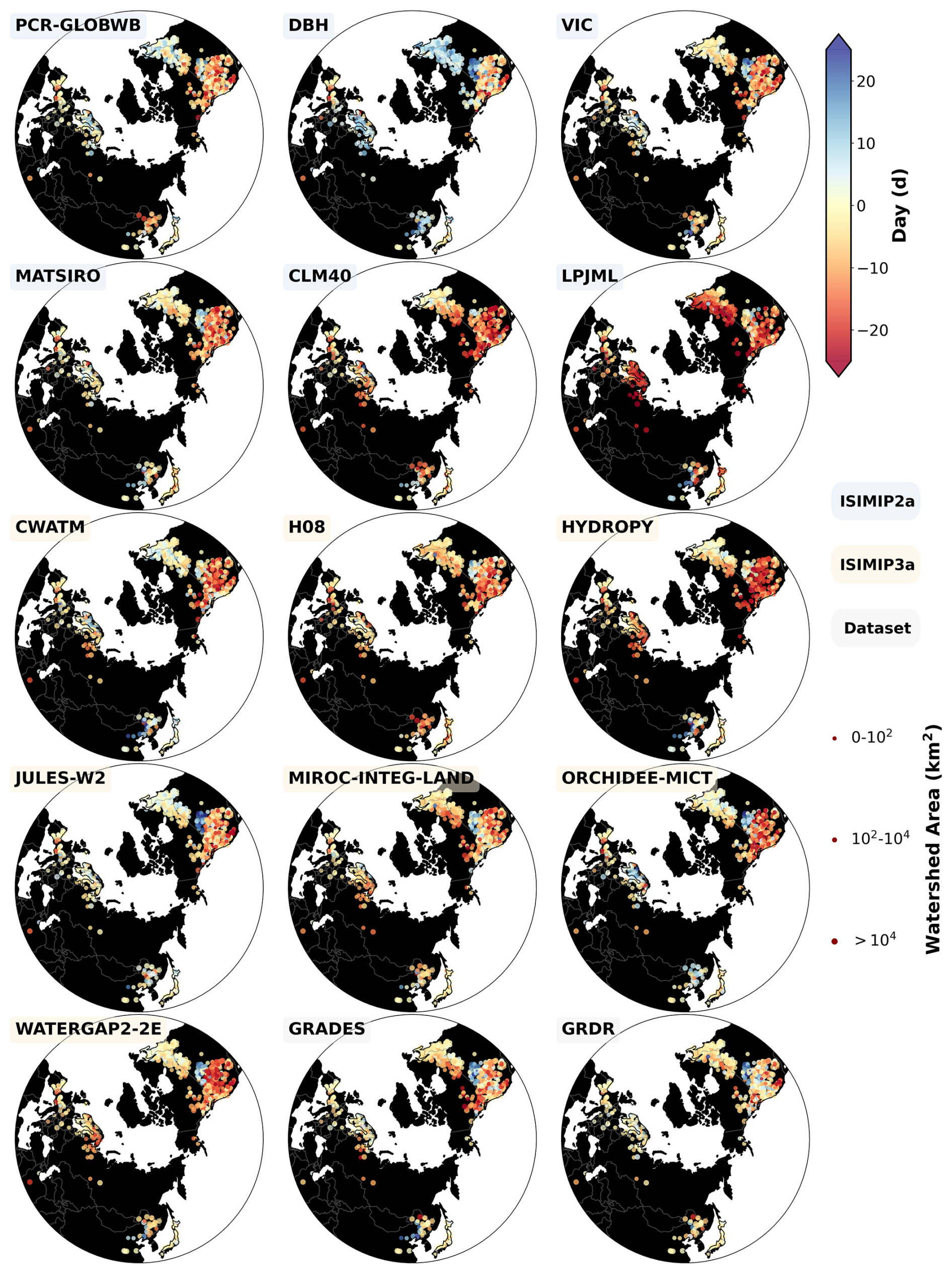
Figure A7 The bias in snowmelt timing, represented by the centroid time of runoff (CTQ) during the snowmelt period (unit: day) Colors indicate the extent of bias compared to observations: red represents earlier snowmelt, blue indicates later snowmelt, and yellow signifies well-matched snowmelt timing. The point size is adjusted based on station density for better visualization and does not have physical significance. Colored boxes around model/dataset names denote three categories of analysis data.

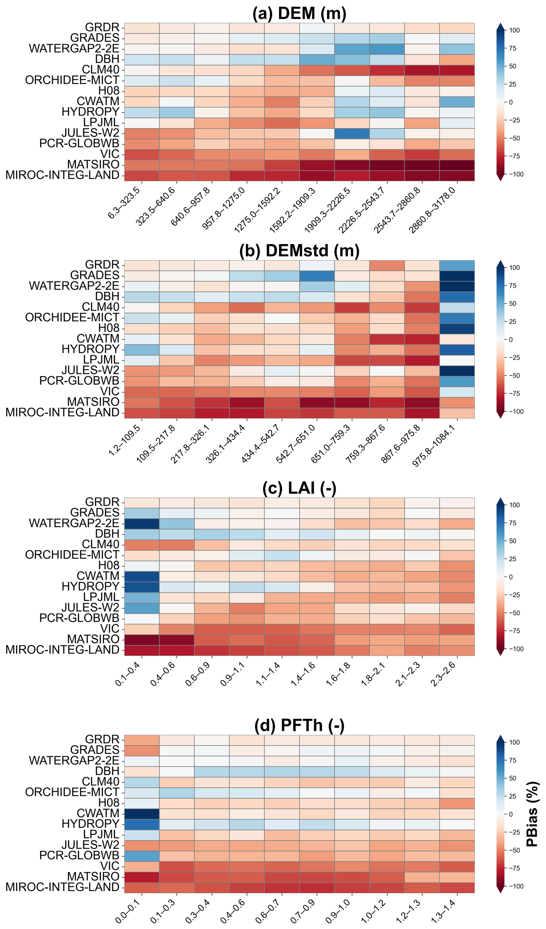
Figure A8 The bias in total runoff (Q_sum) in the snowmelt period as a function of basin complexity factors. The value of each grid represents the median bias (color shading) within the corresponding range of DEM, DEMstd, LAI, and PFTh. The figures are ordered from top to bottom based on the proportion of biases within ±20 %.

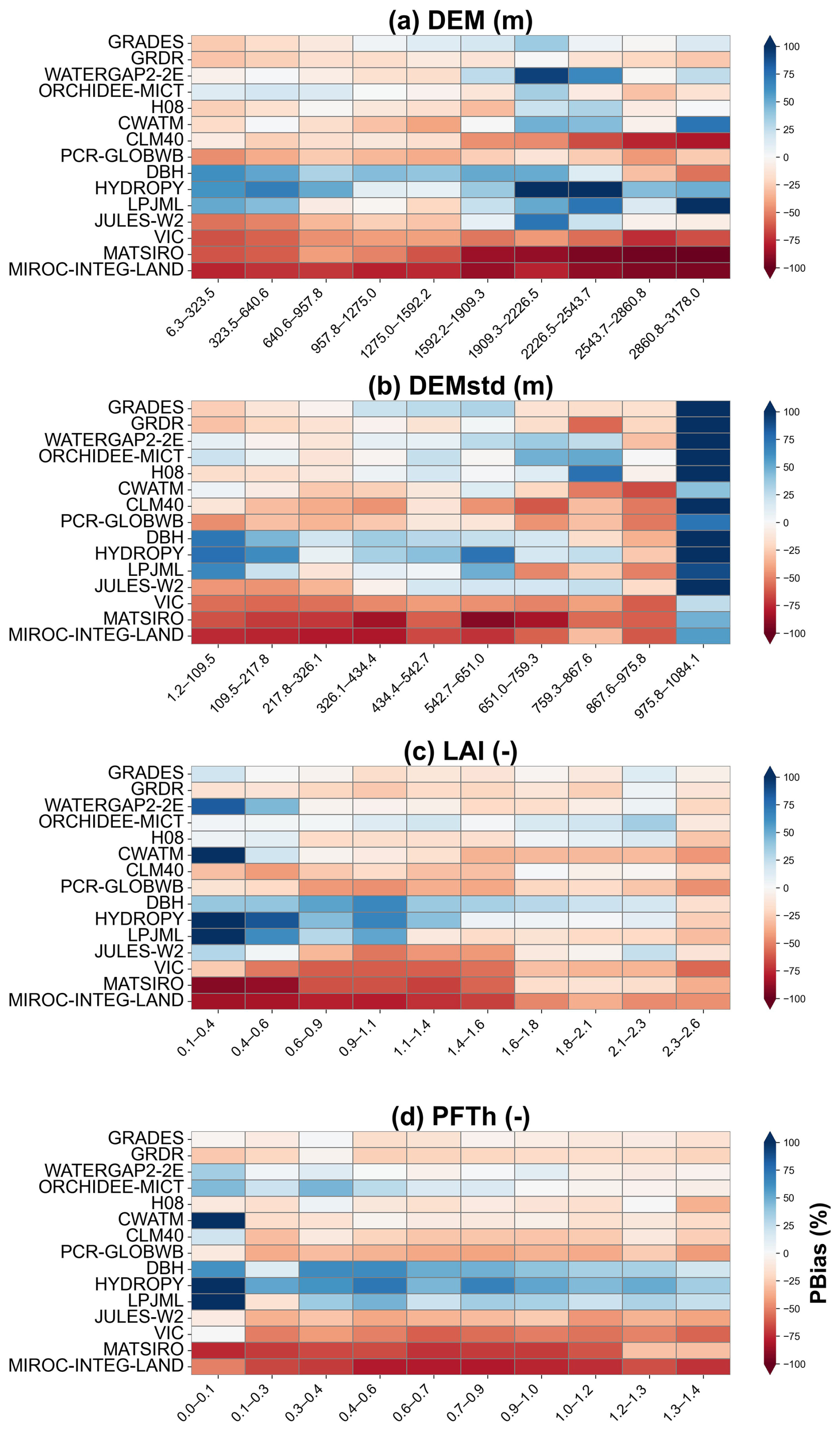
Figure A9 The bias in peak flow (Q_max) in the snowmelt period as a function of basin complexity factors. The value of each grid represents the median bias (color shading) within the corresponding range of DEM, DEMstd, LAI, and PFTh. The figures are ordered from top to bottom based on the proportion of biases within ±20 %.

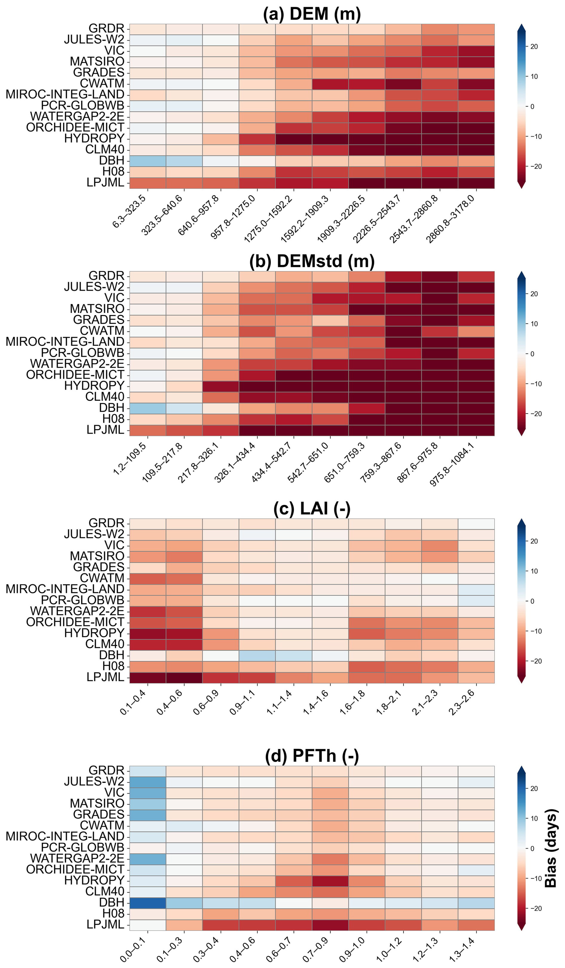
Figure A10 The bias in centroid timing of runoff (CTQ) during in the snowmelt period as a function of basin complexity factors. The value of each grid represents the median bias (color shading) within the corresponding range of DEM, DEMstd, LAI, and PFTh. The figures are ordered from top to bottom based on the proportion of biases within ±5 d.