Retrieving root-zone soil moisture from land surface modelling and GRACE/-FO and validating its dynamics with in-situ data over West Africa

Rainfall variability in West Africa, driven by the West African Monsoon, poses significant challenges to agricultural productivity and livelihoods. In this context, understanding root-zone soil moisture (RZSM) dynamics is crucial since it serves as the primary water source for crops. While surface soil moisture (SSM) has been widely studied, research on RZSM remains limited. This study investigates RZSM dynamics across West Africa from 2003 to 2019 using multiple satellite-derived and model-based datasets, including ESA CCI v0.81, GLWS2.0, WaterGAP, CLM5.0, and in-situ observations. Results indicate that ESA CCI exhibits the strongest temporal and spatial alignment with ground measurements, whereas CLM5.0 and GLWS2.0 effectively capture latitudinal soil moisture (SM) gradients associated with climatic zones. A novel application of an analytical solution to Richards' equation was employed to translate surface moisture signals to deeper soil layers, demonstrating GLWS2.0's superior ability to reproduce seasonal patterns at various depths, notably in Benin and Niger. Despite challenges posed by sparse in-situ data and vegetation-induced signal attenuation, the study highlights the significant benefits of GRACE/-FO data assimilation in enhancing model accuracy. The proposed depth-projection methodology improves the vertical representation of SM, offering new insights into the dynamics of surface and subsurface water storage. These findings have important implications for agricultural forecasting, sustainable water resource management, and climate adaptation strategies in regions where accurate SM data are essential for resilience planning.

1 Introduction

Rainfall in West Africa is largely driven by the West African Monsoon (WAM), characterized by significant spatial and temporal variability (Diatta and Fink, 2014). This variability, often sporadic and unpredictable, increases the region's vulnerability to droughts and floods, severely impacting agricultural productivity and leading to crop failures in rainfed systems (Sonwa et al., 2017; Galle et al., 2018; Myeni et al., 2019). As a result, smallholder farmers, reliant on rainfed agriculture and constrained by financial limitations, face heightened risks to their livelihoods (IPCC, 2023). These challenges significantly hinder economic development and exacerbate poverty in this already vulnerable region, which relies on agriculture for the livelihoods of around 70 % of its estimated 420 million people, with a rapidly growing population at an annual rate of 2.2 %–2.8 % (United Nations Department of Economic and Social Affairs, 2020). RZSM which refers to the amount of water stored in the soil within the root zone of vegetation, typically the top 1–2 m serve as the primary water source for crops (Helman et al., 2019). RZSM directly influences plant growth, agricultural productivity, and water availability for ecosystems (Pegram et al., 2010; Seneviratne et al., 2010; Chartzoulakis and Bertaki, 2015; Helman et al., 2019). Unlike SSM, which can quickly change due to weather conditions, RZSM represents the longer-term water storage available to plants, playing a key role in determining drought resilience and crop yields (Chartzoulakis and Bertaki, 2015). Given that approximately 75 % of the total crop area harvested globally consists of non-irrigated crops (Portmann et al., 2010; Grillakis et al., 2021), the importance of RZSM in global food production and food security becomes even more pronounced. Monitoring RZSM is essential for understanding the water balance (Koster et al., 2004), drought and flood warning (Gavahi et al., 2020; Watson et al., 2022), managing irrigation (Rodríguez-Iturbe and Porporato, 2007; Brocca et al., 2017), and modeling climate impacts on agriculture and natural vegetation (Ruichen et al., 2023). It potentially enhances forecasts and climate projections, guides water resources management, and supports precision agriculture by optimizing water usage.

Currently, SM products (SSM or RZSM) can be generated using three different key approaches: in situ observations, remote sensing, and modelling (Brocca et al., 2017). In situ observations involve ground-based sensors that measure SM directly at specific points using gravimetric, tensiometric and nuclear methods (Myeni et al., 2019). These measurements are reasonably accurate and can capture SM at different depths. However, while in situ observations offer precision, they are labor-intensive and expensive to maintain, and their limited spatial coverage makes them difficult to scale across large regions (Dorigo et al., 2013). This poses challenges in using them for extensive, long-term monitoring over large areas. Nevertheless, the point-scale ground observations are often used as a benchmark for calibrating and validating SM estimates from remote sensing and model simulations (Su et al., 2014; Brocca et al., 2017; Myeni et al., 2019). In recent years, significant efforts have been made to establish in situ SM monitoring networks across Africa, particularly exemplified by the AMMA-CATCH (African Monsoon Multi-disciplinary Analysis–Couplage de l'Atmosphère Tropicale et du Cycle Hydrologique) observatory (Galle et al., 2018). Some of the data collected from these networks have been integrated into the International Soil Moisture Network (ISMN; https://www.ismn.geo.tuwien.ac.at/, last access: 7 June 2026) (Dorigo et al., 2013). These sparse in situ monitoring networks have played a crucial role in validating remotely sensed and simulated SM estimates over extended periods in various African regions (Jung et al., 2019). Remote sensing utilizes various methods, such as microwave, optical, and thermal satellite sensors, to estimate SSM across large areas (Brocca et al., 2017; Myeni et al., 2019). It is an effective technique for detecting the dynamic patterns of SM on regional and global scales. Various satellite instruments, including the Soil Moisture Active Passive (SMAP), Soil Moisture and Ocean Salinity (SMOS), METOP-A/B Advanced Scatterometer (ASCAT), Advanced Microwave Scanning Radiometer–EOS (AMSR-E), and products from the European Space Agency's Climate Change Initiative (ESA CCI), have been successfully utilized to retrieve SSM at a global scale with a temporal resolution of 2 to 3 d (Njoku et al., 2003; Bartalis et al., 2007; Kerr et al., 2012; Entekhabi et al., 2010; Dorigo et al., 2017; Montzka et al., 2017; Chen et al., 2018). While the remote sensing approach offers broad spatial coverage and frequent updates, it primarily measures SM in the uppermost few centimeters (0–5 cm), often missing the deeper root zone dynamics. Additionally, its accuracy can be impacted by factors such as vegetation, weather conditions, radio frequency interference (RFI), and topography, which can reduce measurement reliability. In contrast, the GRACE (Gravity Recovery and Climate Experiment) mission captures changes in total water storage by mapping variations in Earth's gravity field (Tapley et al., 2004). It has been demonstrated that GRACE-observed Total Water Storage Anomalies (TWSA) can be translated into SSM or RZSM using a physically based approach (Grippa et al., 2011; Sadeghi et al., 2020). Although GRACE-based SM data have lower spatial resolution ∼3° vs. 40 km for microwave data and less frequent temporal sampling (monthly vs. daily), data assimilation and downscaling algorithms can be applied to make these two approaches comparable (Gerdener et al., 2023a). Additionally, GRACE data are not affected at all by vegetation density and RFI. This study incorporates this advantage by combining GRACE-based observations with a modelled data approach. The modelled data approach uses simulations that integrate climatic, soil, and vegetation information to estimate both SSM and RZSM across various spatial and temporal scales. Whether based on hydrological or land surface models, both approaches rely on similar equations to simulate SM according a water balance approach (Famiglietti and Wood, 1994). Modelling allows for SM estimates to be generated at high spatial and temporal resolution, offering detailed insights into SM dynamics. However, while models provide comprehensive coverage and long-term predictions, their accuracy is highly dependent on the quality of meteorological input data and the assumptions made in parameterization, which can introduce significant uncertainties. As a result, each modelling approach has its strengths and limitations, and combining multiple methods can provide a more robust and reliable understanding of SM dynamics. While numerous studies have focused on monitoring remotely sensed and modeled SSM data over West Africa (Pellarin et al., 2009a; Pellarin et al., 2009b; Gruhier et al., 2010; Baup et al., 2011; Fatras et al., 2012; Louvet et al., 2015; Faridani et al., 2017) using in situ data, there has been little to no research, to our knowledge, specifically examining RZSM in this region. Furthermore, while the remote sensing products monitored in this area primarily involve AMSR-E satellite data (Pellarin et al., 2009a; Pellarin et al., 2009b; Gruhier et al., 2010), the SMOS satellite mission (Louvet et al., 2015; Jung et al., 2019), and ASCAT satellite data (Jung et al., 2019), SM products based on ESA CCI, CLM5.0, and GRACE/-FO assimilated data have not been comprehensively validated in this region. However, while many physically-based land surface models (e.g., CLM5.0) simulate the SM patterns at different depths by numerically solving Richard's equation, this remains a challenge for conceptual hydrological models. This study aims to retrieve the RZSM from a conceptual model, WaterGAP, as well as the GRACE/-FO-based global assimilation model GLWS2.0 which is based on WaterGAP. The dynamics of these estimates will be validated against in-situ measurements, while additional SM products, including ESA CCI and CLM5.0, will be used for comparative analysis across the West Africa region. This is the first study, to our knowledge, that uses Richard's equation to consistently compare WaterGAP and GLWS2.0 (i.e., GRACE-derived RZSM) to in-situ data sampled at different depths.

Our main research questions addressed in this study are: What is the correlation between the SM from the GRACE/-FO-based global assimilation model (GLWS2.0) and ESA CCI, in-situ data, and other land surface models in the region? How can the water content in the single SM reservoir from the conceptual hydrological models be translated to a SM vertical profile? How does the RZSM changes at each retrieval depth over 2003–2019 in this region? and What is the correlation of its dynamics with the physically-based model (CLM5.0), ESA CCI products, and in-situ data?

The analytical solution of Richards' equation (Sadeghi et al., 2020) will be used to translate water content from the single SM reservoir in GLWS2.0 and WaterGAP to different depths. Our approach offers a distinct advantage over that of Sadeghi et al. (2020), who assumes that GRACE TWSA data have minimal contributions from sources such as groundwater, surface water, or lateral groundwater flow. In their case, any TWSA variation not physically attributable to SM and incompatible with their model is classified as error. By contrast, we work directly with the SM anomaly derived from GLWS2.0 (or WaterGAP), where non-SM components have already been filtered out, offering a cleaner signal for analysis. However, it is important to note that complete separation of these additional hydrological signals from SM may still be imperfect within the assimilation or WaterGAP model. WaterGAP (and thus GLWS2.0) represents SM via a single layer that extends to the root zone. The model simulates varying surface water storages (lakes, wetlands, rivers, and reservoirs) and includes a conceptual groundwater representation. Human water use, i.e. surface and groundwater abstractions, are included in WaterGAP. This approach provides a promising solution to not only expand the shallow vertical support of the microwave satellites with good spatial resolution but also to better isolate the groundwater storage dynamics from the GRACE/-FO-based assimilated signal. This is particularly relevant in West Africa, where SM has been shown to be the dominant component of Total Water Storage (TWS) (Getirana et al., 2017; Jung et al., 2019; Jensen et al., 2024).

2 Study area, datasets and models

2.1 Study area

The study area encompasses West Africa, spanning from 17° W to 17° E and 2° N to 21° N (Fig. 1). The terrain in this region is predominantly low and flat (Tappan et al., 2016). The area is characterized by a latitudinal gradient that includes three bioclimatic regions, progressing from north to south: the Sahelian, Sudanian, and Guinean zones (Galle et al., 2018). This gradient results in varying vegetation patterns (Fig. 2), with the arid north experiencing a single rainy season and sparse vegetation, while the south has two rainy seasons and dense vegetation (Fink et al., 2010). Three meso-scale sites located at different latitudes in Benin, Niger, and Senegal, where AMMA SM observations have undergone advanced quality control procedures by the ISMN, have been selected for analysis in this study (Fig. 1). The Benin site, situated in the Sudanian climate zone, features sandy clay loam soils, woody savanna vegetation, and gently undulating topography (630–225 m above sea level), with about 1200 mm of annual rainfall concentrated in a single rainy season from April to October (Galle et al., 2018). Both the Niger and Senegal sites are located in the Sahel region characterized by a single rainy season between June and October. The Niger site experiences a semi-arid tropical climate, characterized by a long dry season from October to May, with an average yearly temperature of 29.2 °C and 520 mm of annual rainfall (1990–2007) (Galle et al., 2018). The landscape features flat lateritic plateaus and sandy valleys within the Iullemmeden sedimentary basin, which has endorheic hydrology and a continental terminal aquifer. Soils are sandy and weakly structured, contributing to erosion. Additionally, the original woody savannah has transformed into a mosaic of rainfed millet fields and shrubby savannah, mixed with degraded tiger bush vegetation (Cappelaere et al., 2009). The Senegal site, situated in the Dahra region (15.432° W–15.403° N), has a Sahelian climate with a mean yearly temperature of 29 °C, peaking in May, and an annual precipitation of approximately 420 mm. The area features herbaceous vegetation dominated by annual grasses and a tree cover of about 3 %, with most water bodies being temporary, except for a few permanent ponds (Soti et al., 2010; Guilloteau et al., 2014).

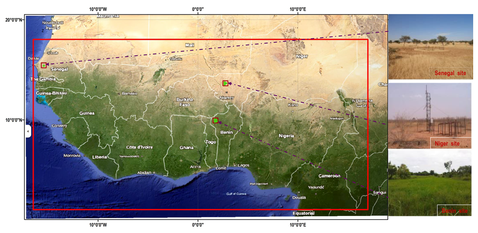
Figure 1 Location of the three meso-scale study sites in West Africa where in situ SM stations from the ISMN are installed: Benin, Niger, and Senegal. Green dots indicate the locations of the individual SM stations (four in Benin, three in Niger, and one in Senegal). Red squares represent the 0.25° satellite grid cells used to compare satellite and model SM products with the in situ observations. The red rectangle delineates the regional domain used for the gridded validation between ESA CCI SM and the land surface models (CLM5.0, GLWS2.0, and WaterGAP). Figure is created by the authors. ISMN data courtesy of ISMN. ESA CCI SM data courtesy of ESA. CLM5.0 data courtesy of NCAR/UCAR. GLWS2.0 data courtesy of the GLWS team. WaterGAP data courtesy of the WaterGAP project. Photos used are adapted from Louvet et al. (2015).

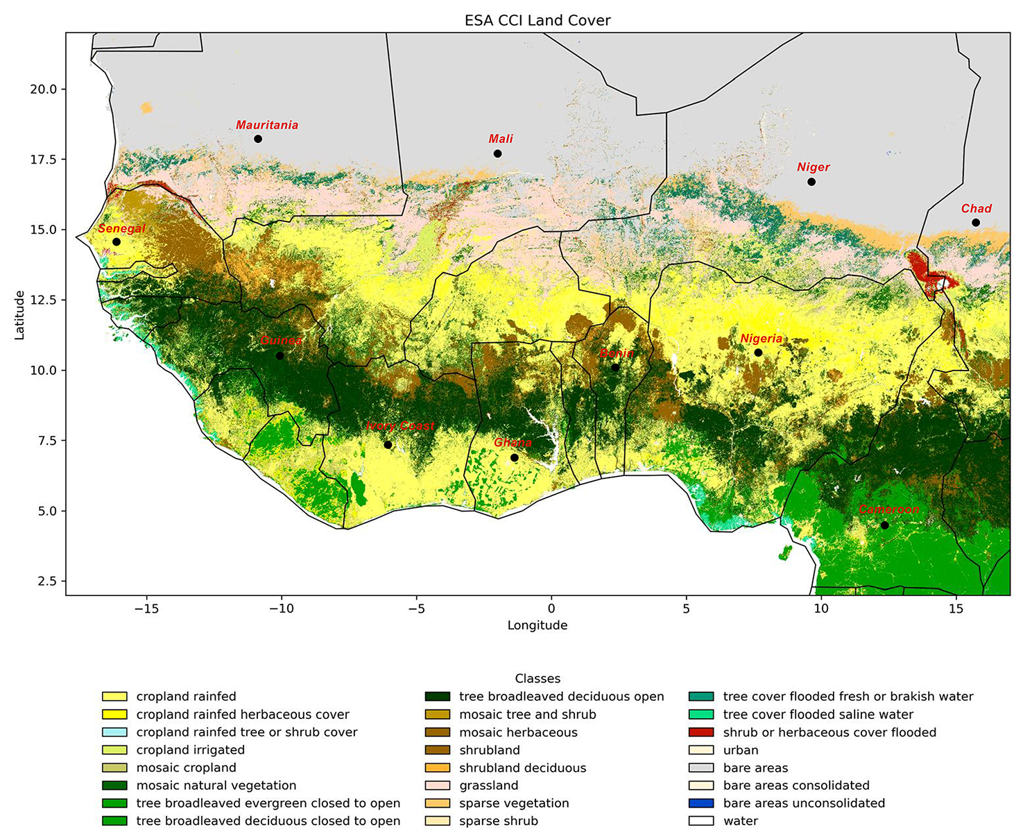
Figure 2 Land cover map over the study area.

2.2 Datasets and models

This section describes the hydrological and land surface models used in this study, and the observational datasets employed for evaluation. Model simulations are forced with homogenized atmospheric reanalysis datasets, including GSWP3-W5E5, CRUNCEP (CRU (Climate Research unit Time Series) (Harris, 2013) and National Centre for Environmental Protection (NCEP) reanalysis (Kalnay et al., 1996), and WFDE5 (WATCH: WATer and global CHange; Forcing Data methodology applied to ERA5 reanalysis data). These datasets offer more spatially sufficient information than direct measurements which are often sparse in Africa.

2.2.1 Hydrological models: WaterGAP and GLWS2.0

This study utilizes version 2.2e of the WaterGAP global hydrology model (Müller Schmied et al., 2021), which simulates daily water fluxes and storage on a 0.5° grid by solving water balance equations across ten water compartments. These compartments represent different storage components within the hydrological cycle, including surface water (rivers, lakes, reservoirs, wetlands), SM, groundwater, snow, glaciers, canopy water, and river floodplains. The model's vertical water balance includes components such as the canopy, snow, and SM, while the lateral water balance accounts for storage in groundwater, lakes, artificial reservoirs, wetlands, and rivers. The vertical water balance is expressed in terms of water height (measured in millimeters), whereas the lateral water balance is calculated using volumetric units (in m³; Müller Schmied et al., 2021). Unlike many land surface models, WaterGAP incorporates human water use for various purposes, including irrigation, livestock, industry, domestic consumption, and cooling of thermal power plants, and is calibrated against long-term annual river discharge. A significant update in this version is the enhanced algorithm for surface and groundwater abstraction. The model employs forcing data from the homogenized GSWP3-W5E5 reanalysis dataset, which includes precipitation, temperature, long-wave radiation, and shortwave radiation (Lange et al., 2022), as well as information on the characteristics of surface water bodies (lakes, reservoirs, and wetlands), land cover, soil type, topography, and irrigated areas. Since its inception in 1996, WaterGAP has been instrumental in assessing the dynamic development of the human-water system, both historically and into the future, particularly in the context of climate change. The model has significantly improved our understanding of changes in continental water storage, with a particular emphasis on the overuse and depletion of water resources (Müller Schmied et al., 2021). GLWS 2.0, or the Global Land Water Storage dataset version 2.0, is developed by assimilating monthly TWSA maps from GRACE and GRACE-FO into the WaterGAP global hydrological model. The Ensemble Kalman Filter (EnKF; Evensen, 2003) was used for assimilation, which is implemented through the Parallel Data Assimilation Framework (PDAF; Nerger and Hiller, 2013). The assimilation process includes vertical disaggregation to optimally combine GRACE/GRACE-FO data with inputs from the hydrological model, resulting in ten distinct water compartments. GLWS 2.0 covers global land areas, excluding Greenland and Antarctica, with a spatial resolution of 0.5° and spans the period from 2003 to 2019, ensuring no gaps in the data. It also incorporates monthly uncertainty quantification at the grid cell level. Key improvements in GLWS 2.0 compared to its predecessor, GLWS 1.0, include the integration of the updated WaterGAP version 2.2e and minor bug fixes in the assimilation process. Comprehensive details about the development of GLWS 2.0 can be found in Gerdener et al. (2023a).

2.2.2 Land Surface Model: CLM5.0

In this study, we use CLM5.0, the latest version of the Community Land Model (CLM), which operates in land-only mode over the Coordinated Regional Climate Downscaling Experiment (CORDEX) Africa domain (Bayat et al., 2023; Oloruntoba et al., 2025). This configuration uses atmospheric reanalysis datasets including GSWP3-W5E5, CRUNCEP, and WFDE5 as external forcings rather than coupling CLM5.0 with an atmospheric model. CLM5.0 simulates key biophysical and biogeochemical processes, such as the interaction between incoming radiation and the canopy/soil, and the exchange of sensible heat, latent heat, and carbon with the atmosphere (Lawrence et al., 2019). Additionally, the model incorporates snow accumulation and melting, along with water and energy transport in the soil. It captures processes such as infiltration, surface runoff, deep percolation, stomatal physiology, and photosynthesis. To account for land surface variability, CLM5.0 divides each grid cell into multiple land units with unique soil or snow columns and plant functional types (PFTs), allowing for a more nuanced representation of surface heterogeneity (Lawrence et al., 2019). Compared to earlier versions like CLM4.5, CLM5.0 provides enhanced accuracy in simulating hydrological and ecological processes and introduces a more explicit representation of human land management, making it a powerful tool for analyzing land-atmosphere interactions and land-use impacts (Lawrence et al., 2019). The model relies on a comprehensive set of atmospheric forcing data, including precipitation, air temperature, shortwave and longwave radiation, specific humidity, surface air pressure, and wind speed. This data is available at different temporal resolutions: every 6 h for CRUNCEP, every 3 h for GSWP, and hourly for WFDE5. It operates at a high horizontal resolution of approximately 0.027° (around 3 km) with a 30 min time step, and output data are further aggregated to a monthly scale for the analysis. SM in CLM5.0 is expressed in volumetric units (cm³ cm⁻³) for each soil layer, structured through a 25-layer soil model extending to a depth of 42 m. Of these, 20 layers are hydrologically and biogeochemically active, providing the simulation of vertical soil water movement through the numerical solution of the Richards equation (Zeng and Decker, 2009). This layered approach improves the model's capacity to capture the vertical distribution of water in the soil, critical for understanding root-zone hydrological processes. For further details on CLM5.0's methods for simulating processes, surface characterization, and vertical soil discretization, refer to Lawrence et al. (2019) and Oloruntoba et al. (2025).

2.2.3 In-situ SM data

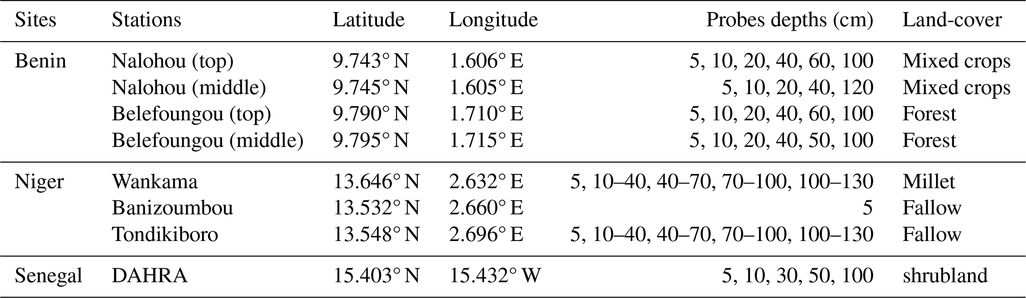
SM observations from three meso-scale sites in Benin, Niger, and Senegal (Fig. 1) spanning from 2003 to 2019 were sourced from the ISMN (Dorigo et al., 2011) to evaluate the accuracy of model-simulated SM in both SSM and RZSM. Table 1 details the geographical coordinates of the SM stations, land-cover types, and the depths of the available SM probes. The locations of the SM stations within the 0.25° satellite pixels are illustrated in Fig. 1. Specifically, there are four stations in Benin (Belefoungou-top, Belefoungou-middle, Nalohou-top, and Nalohou-middle), three stations in Niger (Banizoumbou, Tondikiboro, and Wankama), and one station in Senegal (Dahra). The stations in Benin and Niger are part of the AMMA-CATCH observatory, which monitors land–atmosphere interactions in West Africa (Cappelaere et al., 2009), while the Dahra station in Senegal belongs to the Dahra super-site monitoring ecosystem dynamics in the Sahel (Tagesson et al., 2014). Each SM dataset includes hourly observations in volumetric units (cm³ cm⁻³) at various depths, as outlined in Table 1. Only observations that have undergone rigorous quality control procedures and were flagged as “Good” by the ISMN, were selected for analysis (Dorigo et al., 2013). This ensures that the in-situ data used is of the highest reliability, having passed through stringent checks for accuracy, consistency, and completeness. Additional information regarding the instruments used and the data quality control procedures for the observations can be found in the network reports and the associated references, which are accessible at https://www.ismn.geo.tuwien.ac.at (last access: 7 June 2024). While additional ISMN sites exist in the region (e.g., in Ghana, Nigeria, and Côte d'Ivoire), many were installed relatively recently, primarily within the framework of the Trans-African Hydro-Meteorological Observatory (TAHMO), with most deployments occurring from 2019 onwards. Consequently, these stations do not provide sufficient temporal overlap with our analysis period (2003–2019) and do not meet the temporal coverage and quality requirements for inclusion in this study. By focusing exclusively on the high-quality observations, we aim to minimize errors and uncertainties in the results, leading to more robust and credible findings.

Table 1 Geographic coordinates, stations grouped by site, probe depths, and land-cover types where the probes are installed.

2.2.4 ESA-CCI SM

The ESA-CCI is a global satellite-observed SM dataset developed under the European Space Agency's Climate Change Initiative (CCI). The ESA-CCI SM v0.81 is the latest version data used in this study, providing daily estimates of global SSM, covering the top 2–5 cm of soil, over a long term (1978–2022) at a spatial resolution of 0.25°. The ESA-CCI SSM v0.81 dataset is generated by merging SM data from 12 single-sensor active and 5 passive microwave sensors. For detailed information on the key features of these active and passive microwave sensors, please refer to Gruber et al. (2020). Despite some limitations associated with the chosen merging algorithm and the quality of individual data sources, the v0.81 version has shown significant promise for assessing model performance (Hirschi et al., 2025; Palagiri et al., 2024). In this study, the combined product, which integrates SM retrievals from both active and passive microwave sensors, is selected, as it benefits from the strengths of both types of observations and generally outperforms products that rely solely on single-sensor input (Gruber et al., 2020; Hirschi et al., 2025). The dataset is available free of charge from the ESA website and other platforms, provided in volumetric units (cm³ cm⁻³) and in NetCDF format, making it accessible for long-term climate and hydrological studies. A detailed description of the ESA-CCI SSM product can be found at: http://www.esa-soilmoisture-cci.org/node/139 (last access: 31 August 2024).

2.2.5 Land cover

The land cover data used in this study is sourced from versions v2.0.7cds and v2.1.1 of the ESA CCI Land Cover (LC) dataset, accessed from https://www.esa-landcover-cci.org (last access: 31 August 2024). Version v2.0.7cds covers the period 1992–2015, while v2.1.1 provides data for 2016–2019. However, for this research, the version v2.0.7cds is used for the period 2003–2015, and v2.1.1 for 2016–2019.

The ESA CCI-LC dataset offers global annual land cover maps at a 300 m spatial resolution in NetCDF format, spanning 1992 to 2019. These maps are produced by integrating observations from multiple satellite sensors (e.g., MERIS, SPOT-VGT, PROBA-V) using time-series analysis and supervised machine learning classification based on the Land Cover Classification System (LCCS) (Defourny et al., 2023). The dataset's accuracy has been validated by several studies (Defourny et al., 2023; Chisanga et al., 2024). The land cover map for this study (Fig. 2) was generated by processing NetCDF files, clipping the data to the West Africa region, and calculating the dominant land cover class per pixel for the period 2007–2019, with key land cover types including cropland, tree cover, shrubland, grassland, urban areas, and bare areas.

3 Methods

The methods are organized into four main steps. The detailed procedure for retrieving RZSM from conceptual models (GLWS2.0 and WaterGap) is outlined in Sect. 3.1, while the approach for assessing spatial footprint is discussed in Sect. 3.2. Data pre-processing procedure is covered in Sect. 3.3, and the performance validation approach is presented in Sect. 3.4.

3.1 Projecting RZSM to specific depth

An approach based on the analytical solution of Richards' equation is used to translate the water content from the single SM reservoir in the conceptual hydrological models to different depths. Equation (1) below was applied to retrieve the SM signal at any given depth, following the procedure outlined in (Sadeghi et al., 2020) :

$$\begin{array}{}\text{(1)}& {\displaystyle \frac{\partial \mathit{\theta }}{\partial t}}=D{\displaystyle \frac{{\partial }^{\mathrm{2}}\mathit{\theta }}{\partial z^{\mathrm{2}}}}-k{\displaystyle \frac{\partial \mathit{\theta }}{\partial z}}\end{array}$$

Where θ is the volumetric SM content (cm³ cm⁻³), t is the time (month), z is the soil depth (positive downward; cm), and D is the effective soil water diffusivity (an average value over the entire saturation range; cm² month⁻¹). k represents the average slope of the soil hydraulic conductivity function, which describes the relationship between unsaturated hydraulic conductivity K (cm² month⁻¹) and volumetric SM θ. The soil hydraulic parameters D and K vary with soil type and are calibrated at each site according to the methodology outlined in Sadeghi et al. (2020). Equation (1) illustrates how the SM content, represented by prescribed boundary conditions, changes over time and depth due to soil water diffusion and conductivity. The closed-form solution for determining SM at any arbitrary depth during the Nth time step with time intervals of ΔT (as shown in Eq. 2) is derived by utilizing Warrick (1975) approach to solve Eq. (1). This solution is developed while following the boundary and initial conditions specified in Sadeghi et al. (2020). Eq. (2) is given by:

$$\begin{array}{}\text{(2a)}& {\mathit{\theta }}_N\left(Z\right)=\left\{\begin{array}{l}\begin{array}{rl}& \exp \left(-\mathrm{0.5}Z+\mathrm{0.25}T\right)\\ & F_{\mathrm{1}}U(Z,T)& \text{for}N=\mathrm{1}\end{array}\\ \begin{array}{rl}& \exp \left(-\mathrm{0.5}Z+\mathrm{0.25}T\right)\\ & \mathit{\left\{}{F}_{\mathrm{1}}U\right(Z,T)+{\sum }_{i=\mathrm{2}}^N\\ & \left(F_i-F_{i-\mathrm{1}}\right)U\\ & (Z,\left[N-i+\mathrm{1}\right]\mathrm{\Delta }T)\mathit{\}}& \text{for}N>\mathrm{1}\end{array}\end{array}\right.\end{array}$$

$$\begin{array}{}\text{(2b)}& \begin{array}{rl}U(Z,T)=-\mathrm{0.5}& \exp \left(Z\right)\left(Z+T+\mathrm{1}\right)\\ & \mathrm{erfc}\left[\mathrm{0.5}\left({\displaystyle \frac{Z}{\sqrt{T}}}+\sqrt{T}\right)\right]+\sqrt{{\displaystyle \frac{T}{\mathit{\pi }}}}\\ & \exp \left(-{\left[\mathrm{0.5}\left({\displaystyle \frac{Z}{\sqrt{T}}}-\sqrt{T}\right)\right]}^{\mathrm{2}}\right)\\ +\mathrm{0.5}& \mathrm{erfc}\left[\mathrm{0.5}\left({\displaystyle \frac{Z}{\sqrt{T}}}-\sqrt{T}\right)\right]\end{array}\end{array}$$

where erfc is the complementary error function, N is the total number of discrete time steps, and T, Z and F are dimensionless representations of time t, soil depth z, and net water flux f given by:

$$\begin{array}{}\text{(3)}& \begin{array}{rl}Z& ={\displaystyle \frac{z\cdot k}{D}},\\ T& ={\displaystyle \frac{t\cdot k^{\mathrm{2}}}{D}},\\ F& ={\displaystyle \frac{\left(f-k\cdot {\mathit{\theta }}_{\mathrm{\infty }}\right)}{\left(k\cdot {\mathit{\theta }}_{\mathrm{\infty }}\right)}}.\end{array}\end{array}$$

A closed-form solution is obtained by assuming a stepwise surface flux input F defined as follows:

$$\begin{array}{}\text{(4)}& F\left(T\right)=\left\{\begin{array}{ll}{F}_{\mathrm{1}}& \text{for}\mathrm{0}<T<\mathrm{\Delta }T\\ F_{\mathrm{2}}& \text{for}\mathrm{\Delta }T<T<\mathrm{2}\mathrm{\Delta }T\\ \mathrm{⋮}& \\ F_{\mathrm{N}}& \text{for}\left(N-\mathrm{1}\right)\mathrm{\Delta }T<T<N\mathrm{\Delta }T\end{array}\right.\end{array}$$

θ_∞ as defined in F, represents the long-term temporal mean of relative SM at a given site. The implementation of this approach in our research assumes that the time derivative of the SM component, derived from either the GLWS 2.0 or WaterGAP models, approximates the net water flux f as shown in Eq. (3). Central differencing is employed to avoid introducing a phase lag. This approximation yields the dimensionless flux F, which is used in Eq. (2a). The model is subsequently executed as a sequential computational workflow: first, the monthly single-layer SM time series from GLWS2.0 or WaterGAP is used to compute temporal variations and derive f; second, f is transformed into F (Eq. 3), representing the normalized forcing driving vertical moisture redistribution; third, the analytical solution in Eq. (2) is evaluated for each grid cell, time step, and predefined soil depth to propagate surface moisture variability into deeper layers; finally, the resulting depth-resolved SM profiles are used to compute RZSM by integrating over the corresponding soil layers. The analytical formulation of Eq. (2) enables the computation of the SM profile from GLWS 2.0 or WaterGAP at monthly intervals, eliminating the risk of “truncation error” that can arise in numerical solutions of Richards' equation (Zeng and Decker, 2009). Using this formulation, depth-resolved SM can be derived iteratively for any layer of interest, starting from the surface and proceeding downward through the root zone. Representative values for the soil hydraulic parameters D (diffusion coefficient) and K (slope of the hydraulic conductivity function) are initially assumed, while θ_∞ is set as the long-term average of SSM. These parameters can later be calibrated against in situ observations, using the observed minimum and maximum SM to constrain physically realistic values (Sadeghi et al., 2020). This approach provides a robust and computationally efficient method to translate single-layer SM estimates into full root-zone profiles, facilitating comparison across models, satellite products, and in situ measurements. The SM profile at any desired depth, aligned with the node depths of CLM5 for subsequent comparison, is calculated using Eq. (2).

3.2 Spatial footprint

Spatial footprint, or spatial representativeness, refers to the area surrounding a SM station within which temporal SM dynamics closely align with those observed in nearby regions, as captured in model outputs or remote sensing data. This metric is critical for evaluating a model's ability to accurately reflect local SM dynamics around each station, thereby supporting robust model validation. To understand spatial patterns of SM dynamics in the study area, an insightful approach based on the spatial representativeness is used (Nicolai-Shaw et al., 2015; Orlowsky and Seneviratne, 2014; Molero et al., 2018). This approach quantifies the area surrounding a SM station of interest for which its temporal dynamics are representative, i.e., its spatial footprint. This area is determined by first calculating Spearman's rank-based correlation coefficient between the time-series of the station under investigation and the surrounding pixels of the studied models and then iteratively removing the furthest pixels away from the station of interest, focusing on keeping only those pixels that have a correlation above a predefined threshold (denoted as rcut). The spatial representativeness is ultimately defined by the area covered by the convex hull surrounding these stations that exhibit a correlation above rcut threshold (Molero et al., 2018). A convex hull is the smallest polygon that can enclose all the stations that meet the correlation criteria.

3.3 Pre-processing and performance validation approach of SM products

The SM products used in this study vary in spatial and temporal resolution, layer depths, and units. Consequently, these datasets undergo preprocessing to standardize their specifications for effective comparison through the following steps:

3.3.1 Scaling

To ensure consistency across the different SM products used in this study, a few scaling procedures are applied. First, the SM products have varying spatial resolutions, such as 0.5° for WaterGAP and GLWS2.0, 0.25° for ESA CCI, and 0.2° for CLM5.0. To enable consistent analysis, the outputs from CLM5.0 and ESA CCI are aggregated to match the 0.5° spatial resolution of WaterGAP and GLWS2.0. In addition to this spatial scaling, all datasets are also aggregated to a monthly temporal resolution to align with the standard resolution of GLWS2.0. Second, SM is known to exhibit significant spatial variability, which poses challenges when using single station measurements to accurately represent model simulations across an entire 0.5° SM grid. Direct comparisons between grid-based simulations and point-based observations can introduce substantial errors (Bi et al., 2016). To mitigate this, the study utilizes multiple in situ measurements at each site, which are grouped within the 0.5° × 0.5° model pixel resolution area, covering three sites (Benin, Niger, and Senegal). The average of all SM measurements within each site is computed to provide the best possible approximation of the SM at ground level. This approach, adopted by many authors such as Louvet et al. (2015), Bi et al. (2016), and Zhang et al. (2024), ensures a more reliable comparison. To further refine the process, model values are interpolated to the corresponding in situ points using the nearest neighbor method. Third, another challenge in the validation process is the mismatch in depths between the model-based SM estimates and the SM observations. The ESA CCI captures only near-SSM, whereas CLM5.0 and in situ data provide SM measurements at various depths, including those within the root zone. In contrast, WaterGAP and GLWS2.0 represent the water content within a single SM reservoir spanning the entire root zone. Consequently, these products are not directly comparable in terms of magnitude (Koster et al., 2009). This issue is addressed in Sect. 3.3.2 (Normalization)

3.3.2 Normalization

The soil water simulated by the GLWS2.0 and WaterGAP models, expressed as water depth (in mm), cannot be directly compared to in-situ measurements, ESA CCI data, or CLM5.0 outputs, which are reported in volumetric fraction. For validation purposes, numerous previous studies have used a range of normalization techniques to address the inconsistencies among SM estimates derived from global hydrological models, satellite-based retrievals, and in situ observations (Jung et al., 2019; Tian et al., 2019). Common methods include percentile-based normalization, moving-window anomalies, and statistical rescaling to standardize datasets, improving alignment across diverse sources and enhancing the accuracy of validation analyses. In this study, we employed a percentile-based normalization method using the 2nd and 98th percentiles (Eq. 5).

$$\begin{array}{}\text{(5)}& w_{\mathrm{t}}={\displaystyle \frac{{\mathit{\theta }}_{\mathrm{t}}-{\mathit{\theta }}_{\mathrm{wt}}}{{\mathit{\theta }}_{\mathrm{fc}}-{\mathit{\theta }}_{\mathrm{wt}}}}\end{array}$$

In this approach, each data point in the time series θ_t is normalized by subtracting the 2nd percentile of the entire time series from individual monthly values (θ_wt), followed by dividing the resulting series by the difference between the 98th (θ_fc) and 2nd percentiles of the original time series (θ_wt). θ_wt and θ_fc denote the SM at the wilting point (dry conditions) and at field capacity (wet conditions), respectively. w_t commonly referred to as the Soil Wetness Index (SWI), is widely used in land surface modeling and drought analysis (Noilhan and Planton, 1989; Barbu et al., 2011; Hahn et al., 2026). Its primary purpose is to highlight relative moisture anomalies and drought signals, rather than to represent absolute SM values controlled by soil texture. Values of w_t close to 0 indicating SM conditions approaching the wilting point (dry state) and values close to 1 indicating conditions near field capacity (wet state). This method, commonly referred to as “relative wetness” by Tian et al. (2019) and applied in recent studies (e.g., Tian et al., 2019; Hahn et al., 2026, and references therein), is robust and less sensitive to outliers, making it particularly suitable for our analysis. By normalizing in this way, the approach eliminates information about the original scale, enabling comparisons to focus exclusively on the relative seasonal patterns within each dataset. This avoids biases introduced by absolute magnitudes or imposed statistical alignments, as seen in methods like Raoult et al. (2018), ensuring meaningful comparisons across datasets.

3.3.3 Performance validation approach for SM products

After converting SM simulated in the model and derived from satellites into relative wetness, quantitative evaluations were performed on the refined datasets. The seasonality of different SSM time series is analyzed by applying a 12-month rolling boxcar filter. A boxcar filter is an unweighted moving average filter with a fixed-width temporal window, used to smooth time series by suppressing short-term variability while preserving long-term signals. This approach smooths out short-term fluctuations, effectively isolating long-term variations with periods longer than one year defined here as the seasonal component. Subtracting this smoothed, long-term component from the original time series reveals the residual signal, which captures the episodic variations, defined as short-term SM fluctuations and event-scale anomalies (wet and dry events) occurring on timescales shorter than 1 year.

For the validation of SSM and the ESA CCI grid, only SM probes located at depths ≤ 5 cm were considered to ensure consistency. It was assumed that the microwave retrievals from ESA CCI represent moisture content within the top 0–5 cm of the soil column. Three performance metrics were applied in this study: the Pearson correlation coefficient (R), bias, and root-mean-square error (RMSE) for validating with the in situ data, as well as R and RMSE for grid-based validation using the ESA CCI SM data. R is a key statistical metric in this study, as it assesses how well the temporal variability of in situ and SM product time series align. It remains unaffected by differences in mean or variance, which can arise from varying soil properties or scale discrepancies between in situ data and model or satellite footprints (Koster et al., 2009; Gruber et al., 2020; Beck et al., 2021).

4 Results and Discussion

4.1 Performance validation of SSM products

In this study, we employed two validation approaches. First, we validated SSM products specifically, ESA CCI, GLWS2.0, WaterGAP, and CLM5.0 by comparing model-SM with in situ measurements taken at a depth of 5 cm across different study sites in Benin, Niger, and Senegal. Our analysis emphasized the temporal correspondence between the datasets (e.g., time/phase lags, dry and wet spell event periods) rather than the magnitudes. Dry and wet spells are defined as persistent periods of anomalous SM conditions, corresponding to sequences of consecutive time steps with SM values persistently below or above a defined threshold, respectively. This definition is conceptually consistent with the classical climatological definition of spells as continuous sequences of days with rainfall below or above a given threshold. Additionally, deseasonalized and episodic time series were compared with the corresponding in situ time series to further assess consistency and alignment. Second, we compared the GLWS2.0, WaterGAP, and CLM5 models against the ESA CCI gridded SM data.

4.1.1 In situ-based data validation of different SSM products

The normalized SM time series from ESA CCI, GLWS2.0, WaterGAP, and CLM5.0, along with the in situ time series at each study site are overlaid and presented in Fig. 3. The ESA CCI, GLWS2.0 and CLM5.0 SM products effectively replicate the seasonal dynamics of monthly SSM observed in ground-based measurements across different sites, demonstrating their robustness in capturing the effects of varying land cover and climate conditions in the region. The seasonal changes in SM at a depth of 5 cm show marked variability, likely driven by the influence of the monsoon across the West African region. In situ observations in Niger and Senegal reveal a typical Sahelian seasonal cycle, marked by a distinct wet season from June to October, while the Benin site, located in the Sudanian climate zone, experiences a rainy season extending from April to October, along with a longer monsoon period. More broadly, the dominant role of monsoon systems in controlling seasonal SM dynamics is not unique to West Africa. Similar large-scale monsoon-driven SM cycles have been documented in other monsoon regions, such as the Tibetan Plateau, where SM variability is strongly shaped by the South Asian summer monsoon (Bi et al., 2016). This underscores the importance of regional monsoon systems in determining SM fluctuations across distinct climatic zones. The statistics from the normalized SSM signals, as presented in Table 2, highlight the performance of various datasets in terms of synchronization and correlation with in-situ measurements. In Benin, ESA, GLWS2.0, and WaterGap generally exhibit strong synchronization, with time lags close to 0 months. These datasets also demonstrate high correlations (ESA: 0.894, WaterGap: 0.856, GLWS2.0: 0.752). In Senegal, these same datasets show minimal time lag (ranging from 0 to 1 month), though the correlations are somewhat weaker (ESA: 0.646, WaterGap: 0.637, GLWS2.0: 0.574). In Niger, ESA remains well-aligned with in-situ measurements (0-month lag and a 0.864 correlation), while both GLWS2.0 and WaterGap experience slight delays (1-month lag), accompanied by weaker correlations (0.655 and 0.515, respectively).

Table 2 Statistics from the normalized SSM time series.

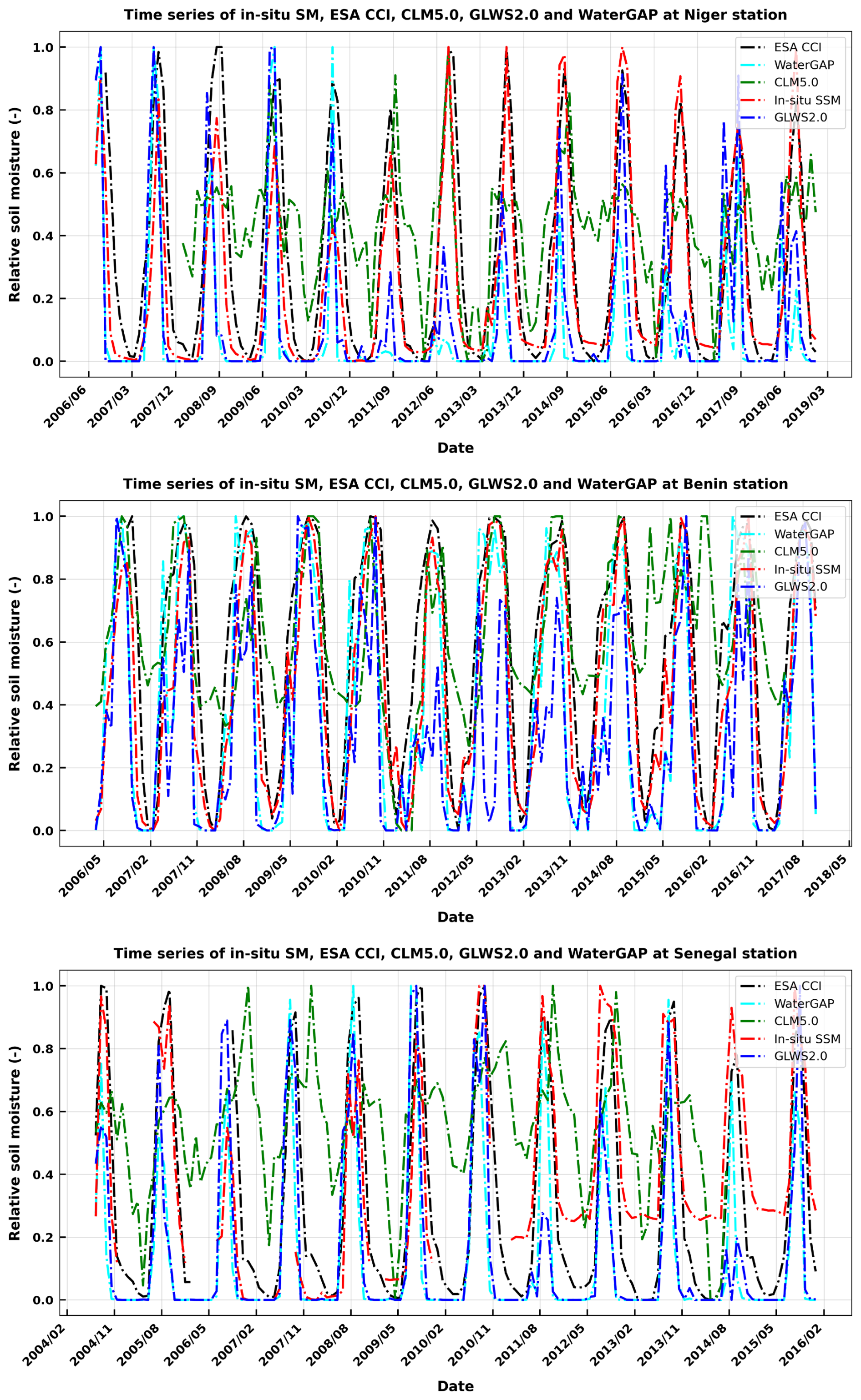
Figure 3 Normalized SM time series for in situ measurements, ESA CCI, GLWS2.0, WaterGAP, and CLM5.0 at three distinct study sites at a depth of 5 cm.

4.1.2 SSM seasonality

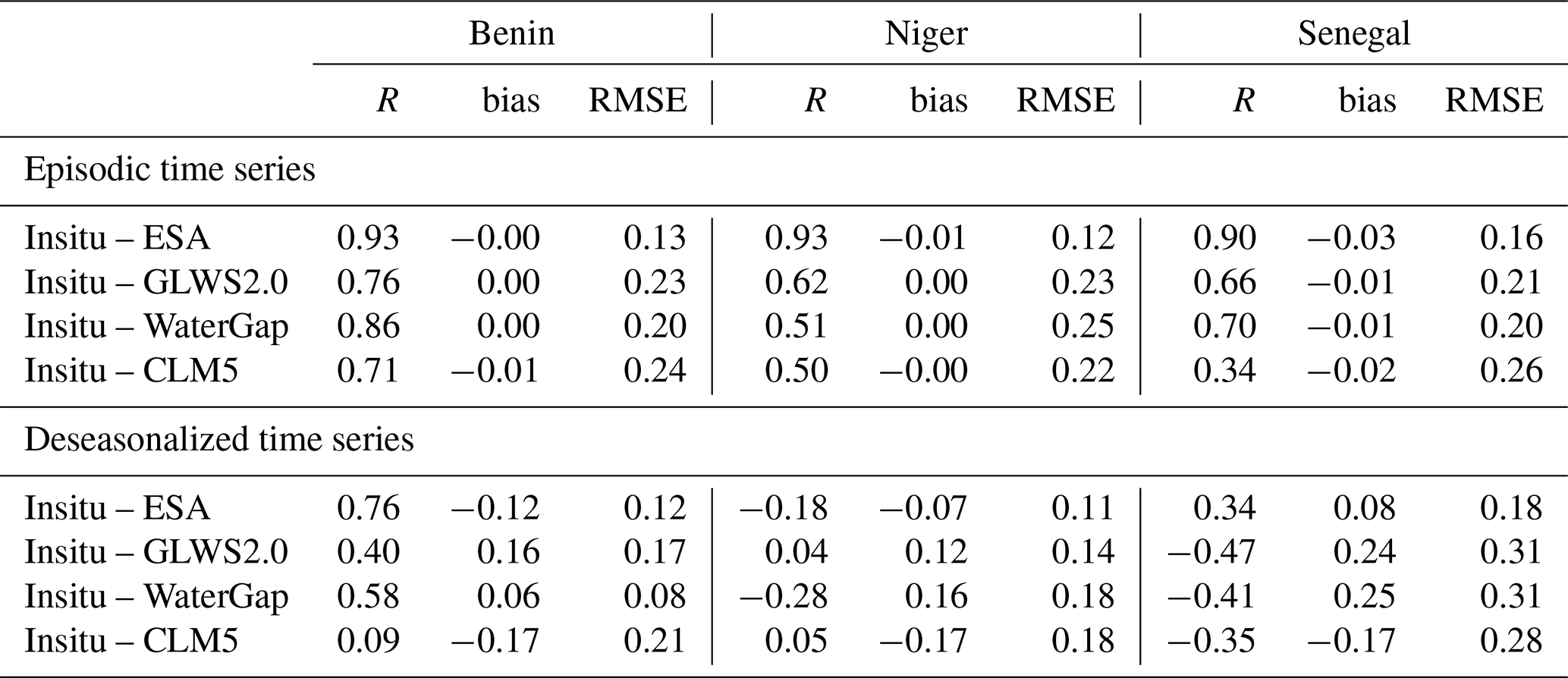
To better highlight events in the time series, a deseasonalization method is applied. The seasonal maps derived from this process are presented in Fig. 4. The statistical characteristics of the episodic and deseasonalized components of the normalized SM time series are summarized in Table 3, providing insights into the magnitude and variability of seasonal patterns and anomalies across the three study sites. The analysis of episodic and deseasonalized time series for SM across Senegal, Niger, and Benin reveals distinct regional patterns influenced by the West African Monsoon (WAM). In the Sahelian zones of Niger and Senegal, typical seasonal cycles show sharp increases in SM during the monsoon (June to October) and declines in the dry season (November to May). Deseasonalized data highlight anomalies, such as unseasonal rainfall or dry spells, which suggest shifts in the timing or intensity of the monsoon and potential impacts of climate variability, such as droughts or flooding.

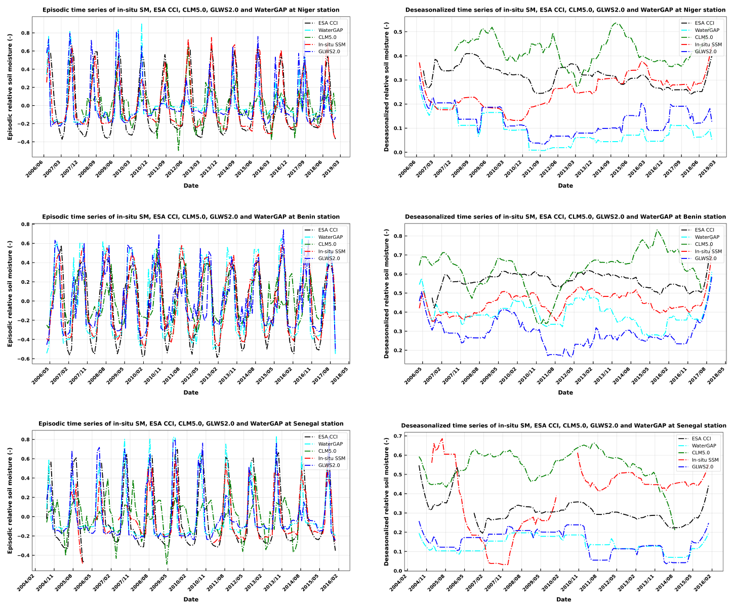
Figure 4 Episodic and deseasonalized SM time series for the three study sites (Niger, Benin, and Senegal).

In Benin, located in the Sudanian climate zone, a longer rainy season (April to October) leads to a more extended period of increased SM, with anomalous events like flooding or unexpected dry spells reflecting changes in rainfall distribution. Overall, deseasonalizing the time series reveals how SM is sensitive to shifts in the monsoon, with delayed rains in the Sahel potentially causing droughts, while early or heavy rains in Benin could lead to flooding or soil saturation. The correlation between the seasonality of the ESA CCI product and the in situ data is generally high, exceeding 0.9 for episodic time series across all sites. At the Benin site, ESA CCI demonstrates the strongest performance, followed by the assimilation-based model GLWS2.0. Meanwhile, at the Niger and Senegal sites, WaterGAP also performs well, ranking closely behind ESA CCI.

Table 3 Statistics of the episodic and deseasonalized components of the normalized SM time series across the Senegal, Niger, and Benin study sites.

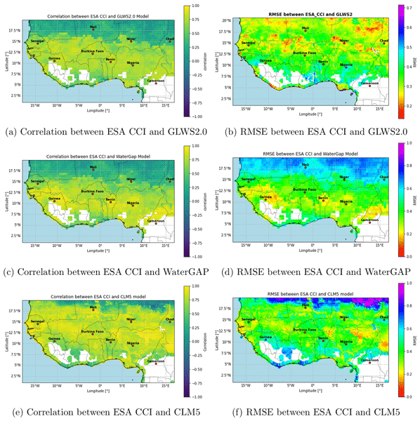
4.1.3 ESA CCI grid based evaluation of the different models

To evaluate the accuracy and performance of the global models used in this study (GLWS2.0, WaterGAP, and CLM5.0) a grid-based comparison was conducted using remotely sensed SSM data from ESA CCI. Figure 5 displays the Pearson correlation coefficient (R) and root-mean-square error (RMSE) metrics, providing insights into how well the GLWS2.0, WaterGAP, and CLM5.0 models perform relative to the ESA CCI grid. In this figure, gaps in the data particularly noticeable in forested and densely vegetated areas (shown as white regions near the coastline) highlight areas where SM estimates are challenging. This data masking in the ESA CCI SSM datasets occurs because microwave-based observations typically exclude areas with moderate to dense vegetation due to the strong attenuation of soil signals by the vegetation canopy (Dorigo et al., 2017).

Figure 5 also reveals that the patterns in RMSE and correlation metrics vary with land cover type, demonstrating that land cover exerts a clear influence on the performance of these models. GLWS2.0 shows a notably lower RMSE than the other models across the region and exhibits strong spatial consistency across various land cover types. The lowest RMSE values for GLWS2.0 are observed in the semi-arid Sahel regions, likely due to its effective assimilation process that better captures SM dynamics in these environments.

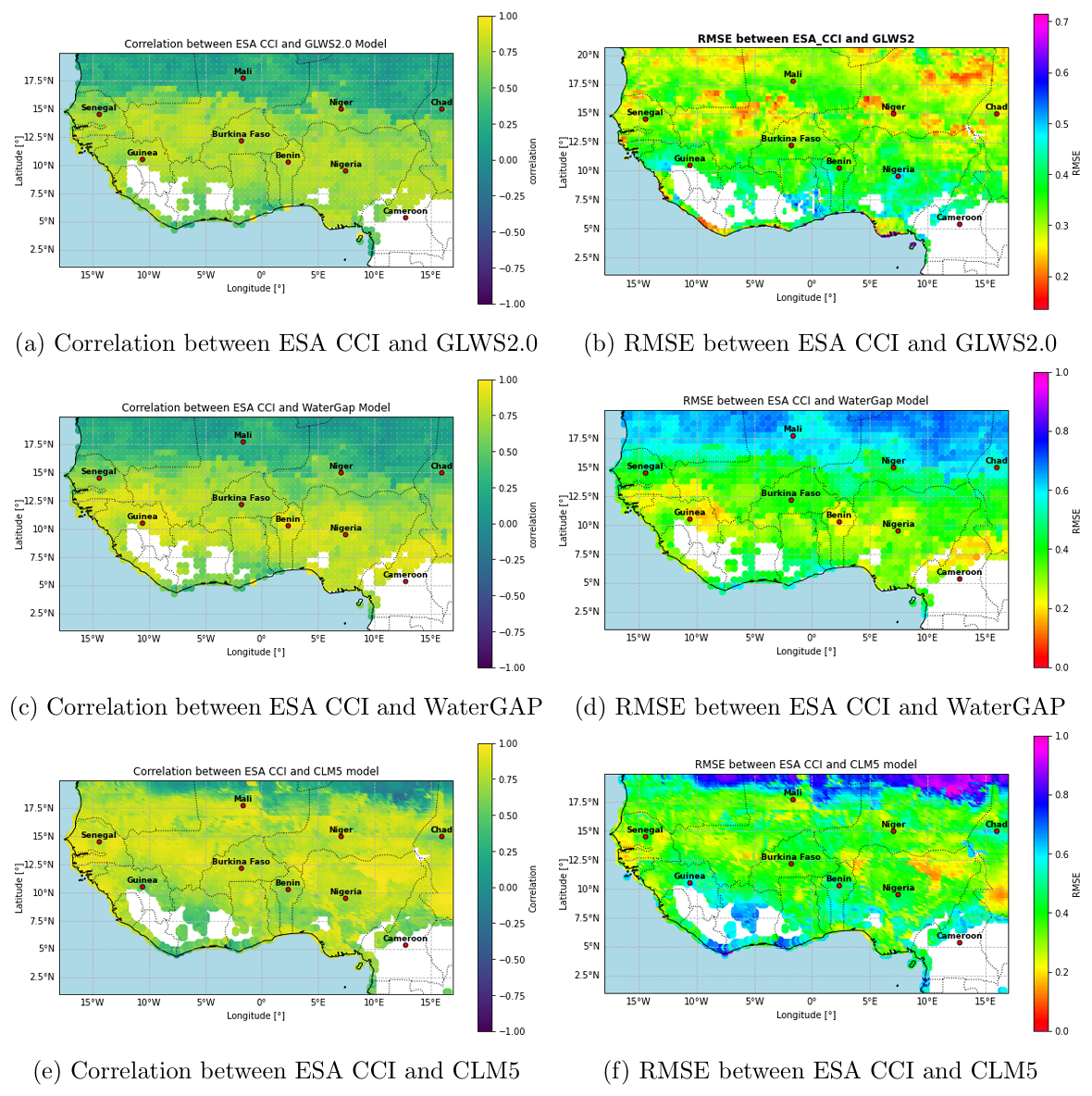
Figure 5 Pearson correlation coefficient (R) and RMSE metrics illustrating the performance of GLWS2.0, WaterGAP, and CLM5 models relative to the ESA CCI grid. Figure created by the authors using datasets described in the manuscript.

The figure underscores the complexities of SM modeling across the diverse climates and land covers of the West African region, where model performance and error metrics vary significantly. While GLWS2.0 demonstrates spatial consistency across different land-cover types with relatively low RMSE values, this consistency is not as evident in other models. RMSE values are generally lower in the northern part of West Africa but higher in the southern regions. This variation may be attributed to the sporadic nature of SM in these areas, where conditions are highly dependent on occasional rainfall events. In these regions, SM levels can shift rapidly, with dry conditions prevailing and only brief, intense increases in moisture following rainfall. Both the satellite data (ESA CCI) and the hydrological models encounter challenges in accurately capturing these short-lived, extreme moisture events. However, because arid and semi-arid regions experience prolonged dry spells, the overall RMSE between model predictions and satellite observations remains relatively low, despite the missed short-term fluctuations. This pattern underscores the inherent challenges of modeling SM in arid and semi-arid regions, where infrequent but intense moisture changes add complexity to the dynamics. Additionally, the figures show that GLWS2.0 demonstrates a stronger correlation with ESA CCI data compared to the WaterGAP model, which does not exhibit a clear dependency on land-cover types. Although the correlation between ESA CCI and CLM5.0 appears to be the strongest overall, the RMSE values for GLWS2.0 are slightly more favorable in arid and semi-arid regions. This correlation is generally higher in southern West Africa and weaker in the north, where low SM values make it difficult to discern clear patterns. In the southern regions, more frequent and consistent rainfall leads to stable SM levels, allowing moisture dynamics to be easier to predict. Consequently, the spatial correlation pattern between GLWS2.0 and ESA CCI SM data reveals a clear latitudinal gradient aligned with annual rainfall and climate zones. This pattern is particularly evident in semi-arid regions that serve as transition zones between wet and dry climates, where the highest correlation values are observed (i.e. area between 9.5 and 15° N). Such transitional regions, including the Indian subcontinent, the North American Great Plains, and southeastern Brazil, also exhibit increased correlation values due to pronounced seasonal and inter-annual variability in SM measurements (Al-Yaari et al., 2014). Similar findings were reported by Jung et al. (2019) over West Africa, where an evaluation of spatial correlations between GRACE-based assimilation, SSM simulations and satellite-derived SSM products (ASCAT, SMOS, and SMAP) indicated strong correlation patterns in transitional zones. This consistency suggests that SM measurements in these regions are particularly sensitive to seasonal dynamics and the distinct cycles of wet and dry phases. Moreover, GLWS2.0 effectively captures the general pattern of SM in the south, where soils retain moisture better and vegetation moderates fluctuations.

4.2 Spatial Representativeness

Figure 6 illustrates the Spatial Representativeness (SR) of ESA CCI, GLWS2.0, WaterGAP, and CLM5.0 using a cutoff Spearman correlation of 0.6, which effectively highlights how well each SM product reflects observed SM dynamics at each study site. This similarity threshold distinguishes between datasets that demonstrate moderate to strong agreement with in situ observations, categorizing them as performing well (correlation > 0.6) or less effectively (correlation ≤ 0.6) in capturing real-world variations. Notably, only ESA CCI and GLWS2.0 exhibit Spearman correlations greater than 0.6 with in situ data, indicating that these datasets accurately capture the spatial and temporal dynamics of SM within their respective spatial footprints. This alignment suggests that their SM estimates correlate quite well with the observed time series. Furthermore, the efficacy of the GLWS2.0 assimilation process likely enhances its ability to reflect real-world SM conditions, particularly in arid and semi-arid regions characterized by sporadic moisture changes. In contrast, the lower correlations observed for WaterGAP and CLM5.0 point to limitations in these models' capacity to represent SM variability at finer spatial scales. Overall, these findings underscore the importance of integrating observational data to enhance model accuracy in representing high-resolution SM dynamics, suggesting that ESA CCI and GLWS2.0 are better suited for regional applications requiring high spatial sensitivity. Although the SR approach has not previously been applied to the satellite/model SM products examined in this study, it has proven effective for validating other SM products across various regions worldwide. For example, in the Little Washita watershed in the United States and the Yanco area in Australia, spatial representativeness has been used to explore the connections between SM spatial scales and timescales within the  50 km satellite footprint of SMOS, AMSR2, and ECMWF SM products (Molero et al., 2018). These authors demonstrate that the spatial representativeness of SSM increases with longer timescales, but with greater variability in these regions. Nicolai-Shaw et al. (2015) showcased the robustness and effectiveness of this approach for selecting appropriate SM products. By applying it to analyze the temporal dynamics of absolute SM across North America, they compared in situ observations with the European Space Agency's ECV-SM and ERA-Land datasets. Orlowsky and Seneviratne (2014) demonstrating the robustness of this parameter-free method in climatology to quantify the spatial footprint of weather stations across Europe. Their findings show that temperature data generally exhibit greater representativeness than precipitation, with significant seasonal changes influenced by atmospheric circulation patterns, particularly in boreal winter.

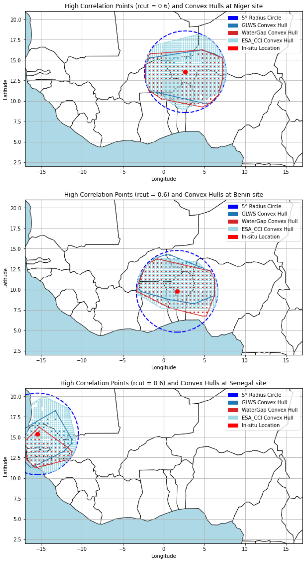
Figure 6 Spatial footprint of SM products represented by a blue circle with a radius of 5° around each site, indicated in red. The convex hulls in light and dark blue represent the areas for which ESA CCI and GLWS2.0 exceed the specified cutoff threshold of 0.6, respectively. Figure created by the authors using datasets described in the manuscript. ESA CCI data courtesy of ESA. GLWS2.0 data courtesy of the GLWS team. WaterGAP data courtesy of the WaterGAP project. CLM5 data courtesy of NCAR/UCAR.

4.3 Retrieving the RZSM from GLWS2.0 and WaterGap and validating its dynamics using in-situ and CLM5

An analytical solution to Richards' equation is used to convert water content from GLWS2.0 and WaterGAP to different depths, enabling comparison of model-derived RZSM with in-situ observations across depths (Figs. 7 to 9).

At shallow depth (5 cm), GLWS2.0, which incorporates GRACE/FO data, demonstrates superior performance than WaterGAP and yields results comparable to those of CLM5.0 in capturing the monthly RZSM dynamics at the Niger and Benin sites (Fig. 7). However, the temporal dynamics at the Senegal site are less consistent, particularly during the initial 2 years (2004–2006) of the in situ observation system. This discrepancy can be partially attributed to the Senegal site being represented by a single station, unlike Niger and Benin, which have at least three stations at different locations. The limited data from a single station poses challenges in accurately representing model simulations over a broader 0.5° SM grid study (Louvet et al., 2015). Furthermore, the WaterGAP model struggles to capture long-term (2006–2018) seasonal dynamics at all sites as recorded by in situ sensors. At this depth, a comparison of model performances in capturing seasonal SM dynamics shows that the ESA CCI model aligns most closely with in situ measurements. ESA CCI achieves the lowest RMSE and the highest R² values across all study sites: Benin (RMSE = 0.19, R²= 0.71), Niger (RMSE= 0.17, R²= 0.66), and Senegal (RMSE = 0.21, R²= 0.53). The GLWS2.0 assimilation-based model ranks second in accuracy, with corresponding values in Benin (RMSE = 0.33, R²= 0.22), Niger (RMSE = 0.32, R²= −0.03), and Senegal (RMSE = 0.31, R²= 0.40). CLM5.0 provides performance metrics similar to those of GLWS2.0, with values in Benin (RMSE = 0.34, R²= 0.24), Niger (RMSE = 0.34, R²= −0.35), and Senegal (RMSE = 0.386, R²= 0.26). These results indicate that ESA CCI demonstrates the highest accuracy in reflecting seasonal SM patterns, while GLWS2.0 and CLM5.0 show comparable but lower precision in fitting observed in situ measurements across all sites.

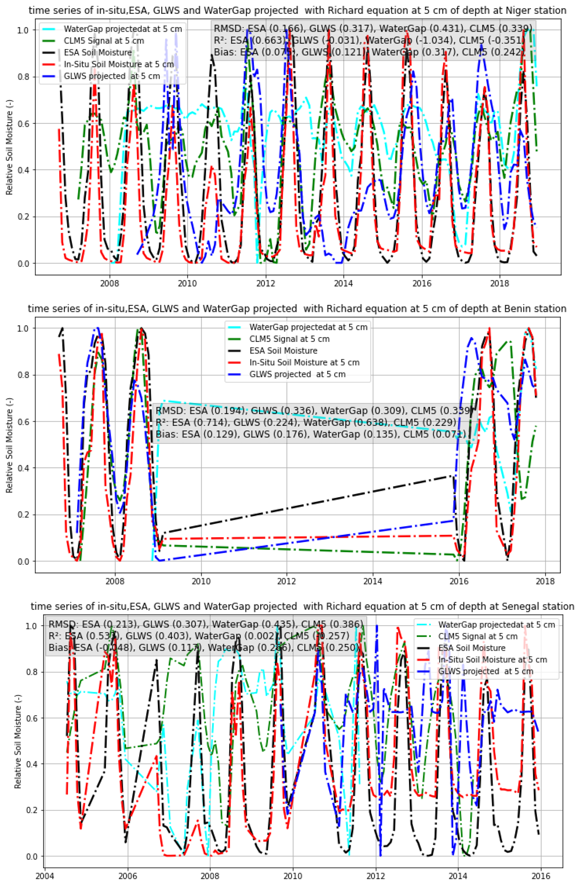
Figure 7 SM time series for in situ measurements, ESA CCI, GLWS2.0, WaterGAP, and CLM5.0 at three distinct study sites, projected at a depth of 5 cm. ESA CCI data courtesy of ESA. GLWS2.0 data courtesy of the GLWS team. WaterGAP data courtesy of the WaterGAP project.

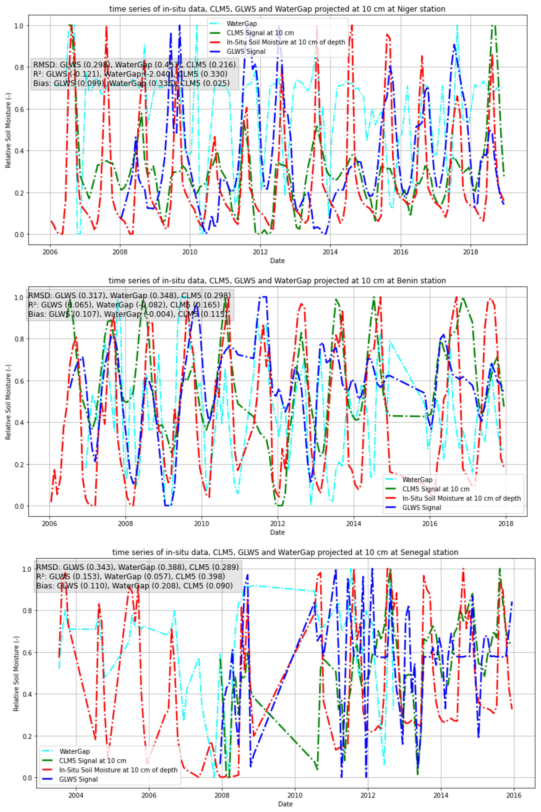
Figure 8 SM time series for in situ measurements, ESA CCI, GLWS2.0, WaterGAP, and CLM5.0 at three distinct study sites, projected at a depth of 10 cm.

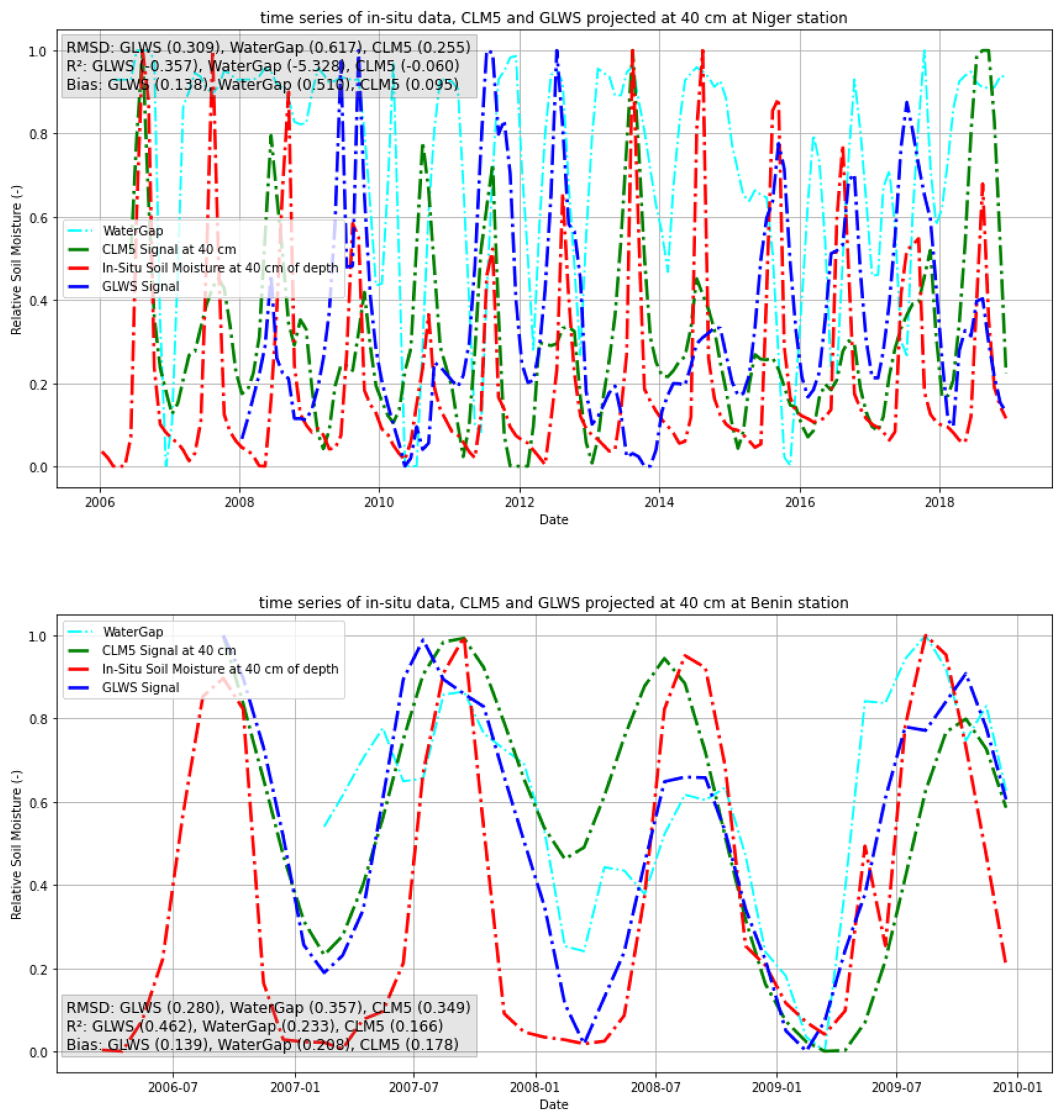
Figure 9 SM time series for in situ measurements, ESA CCI, GLWS2.0, WaterGAP, and CLM5.0 at different study sites, projected at a depth of 40 cm.

Extending the analysis to deeper layers (10, 40, and 100 cm) as illustrated in Figs. 8, 9, and 10, which represent RZSM at these depths, both GLWS2.0 and CLM5.0 capture reasonably the seasonal dynamics of SM at the Niger and Benin sites. These models show good alignment with in situ measurements across different depths, demonstrating their ability to reflect seasonal moisture changes as recorded by the local sensors. However, the WaterGAP model does not reflect this seasonality effectively. At the Senegal site, these seasonal patterns are notably absent, likely due to previously mentioned issues with the limited data from a single station, which may not fully represent local SM variability at the model's grid scale (0.5° resolution).

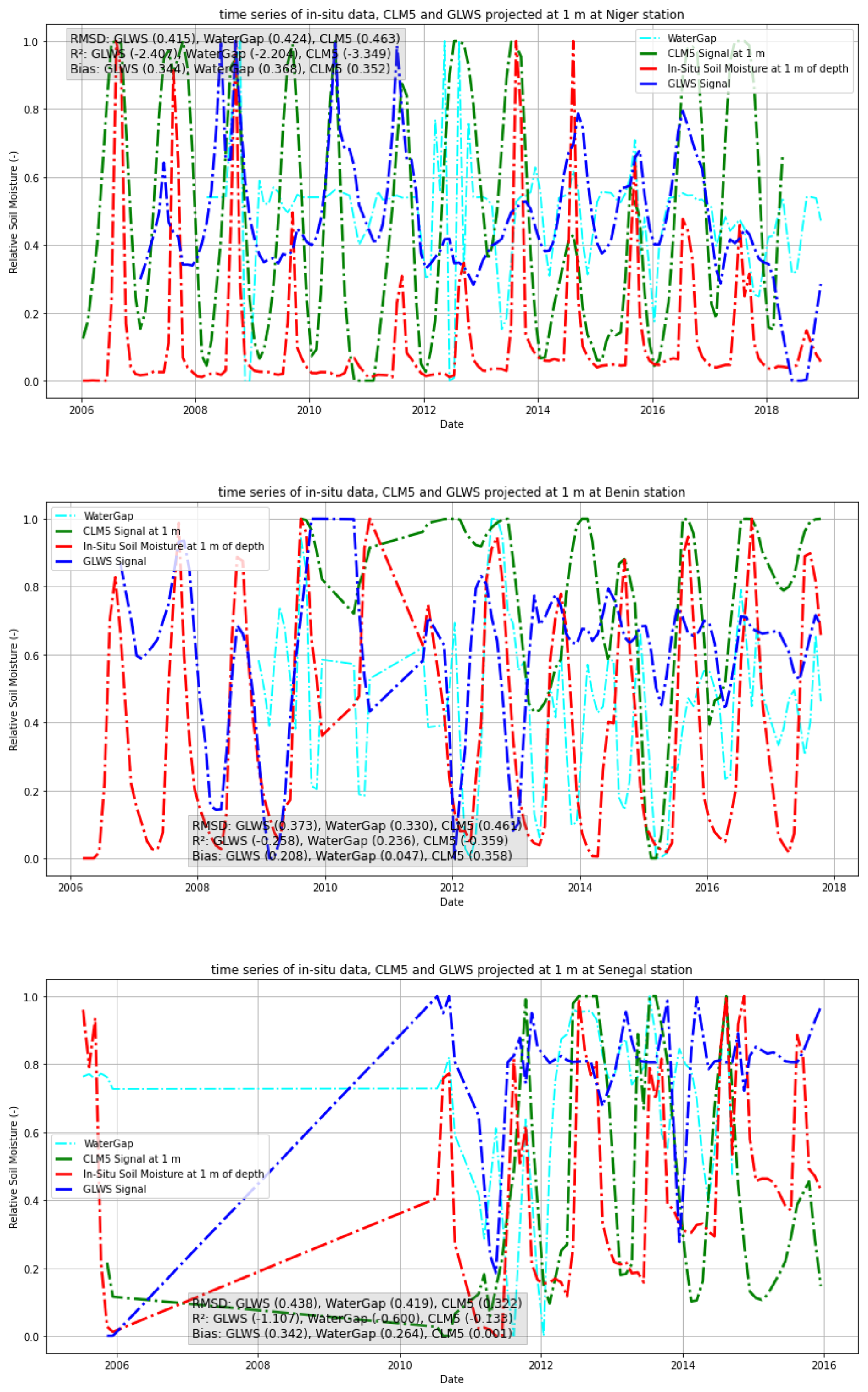
Figure 10 SM time series for in situ measurements, ESA CCI, GLWS2.0, WaterGAP, and CLM5.0 at three distinct study sites, projected at a depth of 100 cm.

Furthermore, seasonal consistency in GLWS2.0 projections across depths is less reliable at the Senegal site, situated near the coastline. This discrepancy could stem from coastal regions' unique characteristics, such as tidal influences and potential signal interference from the nearby ocean, which may impact the accuracy of GRACE/-FO-based observations used in the model's assimilation process. In comparing RZSM estimates retrieved from GLWS2.0 and WaterGAP to in situ observations and the physically based model CLM5.0 at depths of 10 and 40 cm, CLM5.0 demonstrates slightly better performance. This is reflected in CLM5.0's smaller RMSE and higher R² values across the study sites, indicating a closer alignment with observed moisture dynamics. However, at a depth of 100 cm, GLWS2.0 performs marginally better than CLM5.0, with slightly lower RMSE and higher R² metrics, suggesting a potential advantage of GLWS2.0 in capturing RZSM dynamics at this depth. Overall, while GLWS2.0 exhibits solid performance, particularly in comparison to WaterGAP, WaterGAP's RZSM estimates show more significant discrepancies from both in situ measurements and the results provided by CLM5.0, especially at all depths observed. In addition, CLM5.0 performed quite poor at 5 cm, but relatively good at greater depths. This might be related to inclusion of measurement data by ESA CCI at 5 cm, while CLM5.0 did not have data assimilation at this depth. The influence of 5 cm SM measurements diminishes at greater depths, while apparently the model for vertical SM transport scheme that CLM5.0 uses is better than for the other models. GLWS2.0, on the other hand, benefits from GRACE-based data assimilation at depth, which likely explains its comparatively stronger performance at 100 cm.

5 Conclusions and implications

This study assessed RZSM dynamics across West Africa (2003–2019) using GLWS2.0, WaterGAP, CLM5.0, ESA CCI v0.81, and in-situ measurements. Overall, ESA CCI shows the strongest temporal agreement with in situ data, characterized by near-zero time lags and consistently high correlations across all regions. CLM5.0 and GLWS2.0 show moderate to good performance, whereas WaterGAP performs less reliably. A grid-based validation reveals that CLM5.0 and GLWS2.0 correlate more strongly with ESA CCI across West Africa, displaying a distinct latitudinal gradient aligned with annual rainfall and climate zones. This gradient is particularly strong in the transition zones between wet and dry climates (9.5 to 15° N). In contrast, WaterGAP lacks this dependency on land-cover types, suggesting its limitations in capturing regional SM variations. To evaluate how well each product captures spatially coherent SM dynamics, a Spearman correlation threshold of 0.6 was applied. The results show that ESA CCI, GLWS2.0, and CLM5.0 consistently meet this threshold around the studied sites, indicating that these models accurately capture the spatial and temporal dynamics of SM within their respective spatial footprints. However, it is important to acknowledge several limitations that may affect both the in-situ and grid-based validation, as well as the spatial footprint analysis. First, the limited number of in-situ probes at each study site may not adequately capture the local variability in SM, especially when compared to the coarser 0.5° spatial resolution of the models. Additionally, the availability of ESA CCI data is often restricted in forested and densely vegetated regions due to the strong attenuation of microwave signals by vegetation canopies, as noted by Dorigo et al. (2017). Another source of uncertainty lies in the mismatch between the spatial representativeness of point-based observations and the model grid size, which can introduce discrepancies in the validation process. Moreover, the normalization applied to the datasets, while useful for comparative purposes, may have masked true differences in SM magnitudes across products. Finally, temporal gaps in data coverage whether in in-situ records or satellite-derived products can affect the consistency and reliability of the validation outcomes.

The analytical solution of Richards' equation used to translate water content from a single SM reservoir to various depths provides additional insights into vertical SM dynamics. GLWS2.0 performs better than WaterGAP at depth, largely due to GRACE/-FO data assimilation, while CLM5.0 also shows robust performance despite not assimilating GRACE/-FO data. The novel application of this depth-translation approach, based on analytical solutions of Richards' equation, enabled the projection of water content from a single SM reservoir to various depths across West Africa, providing insights that go beyond traditional SM analysis in the region. This methodology not only extends the shallow vertical range typically captured by microwave satellite sensors, but it also offers a way to differentiate surface and groundwater storage variations within the GRACE/-FO data, potentially expanding our understanding of water storage dynamics in complex hydrological settings. We acknowledge that the analytical solution of the Richards' equation represents a simplification of reality. Implementing a more refined (numerical) version, together with more detailed representations of soil types, plant root water uptake, and soil hydraulics, would actually require taking steps towards assimilating GRACE data into more refined land surface hydrology models. We believe this should be explored in future studies (Springer et al., 2026). By enhancing the representation of SM across different depths, this framework can improve agricultural forecasting and deepen our understanding of water cycle interactions across diverse landscapes, especially in regions where accurate SM data are essential for sustainable water management.