Technical note: Temperature dependence of precipitation tail heaviness in the TENAX model

Climate change is causing the magnitudes of extreme sub-daily precipitation events to increase. The ability to predict changes to these precipitation extremes is crucial for disaster preparedness. The TENAX model was proposed to predict return levels of sub-daily extreme precipitation under climate change based on the projected temperature shifts. It combines a Weibull distribution with an exponential temperature dependence in the scale parameter, accounting for the Clausius–Clapeyron relation, with an explicit representation of the temperatures during precipitation events. The Weibull distribution's shape parameter could also have a temperature dependence, which would mean that the tail heaviness changes with temperature. This implies that the rarest events may increase at faster rates. However, implementing this dependence increases the number of parameters to be estimated, affecting the model's accuracy. Here, we use hourly data from thousands of rain gauges in Germany, Japan, the UK, and the USA to assess the dependence of the Weibull shape parameter on temperature, exploring how it should be implemented in the TENAX model. We find that there is a significant dependence in many stations and that the magnitude and sign of the dependence have regional patterns. In the majority of stations, the sign is negative, implying that rarer events intensify with temperature at a higher rate. However, Monte Carlo simulations show that including this dependence without careful consideration may lead to overestimation of precipitation return levels and increase the model uncertainty. The dependence should therefore be introduced with caution, in the context of surrounding stations.

1 Introduction

Extreme sub-daily precipitation leads to natural hazards such as urban floods, debris flows, and flash flooding. For example, in July 2025, Texas experienced a severe precipitation event, with 130 to 280 mm of rainfall recorded in under 12 h, resulting in flash floods that claimed the lives of over 130 people (Adams, 2025). Record-breaking intermittent heavy rainfall on the southern Japanese island Kyushu caused floods and landslides, resulting in over 60 deaths (Digital Archives of Kumamoto Disasters, 2021). The southern UK town of Boscastle saw a damaging but non-fatal flood in 2004 caused by extreme localised rainfall. In one location, 86 mm of rain was recorded in 1 h (Burt, 2005). Extreme events such as these are often discussed in relation to anthropogenic climate change (Pall et al., 2011; Faranda et al., 2025; Kawase et al., 2020). It is difficult to attribute individual extreme events directly to climate change, but they are rarely seen in the historical record and are expected to increase in frequency and magnitude in the future (Fowler et al., 2021; Ebers et al., 2024; O'Gorman, 2015).

The intensification of extreme short-duration precipitation with temperature is assumed to follow the increase of atmospheric water vapour, which follows the Clausius-Clapeyron relationship, pointing to a potential intensification of 7 % °C⁻¹ in ideal atmospheric conditions (Trenberth et al., 2003). However, observational studies have found that extreme precipitation may scale with temperature differently than this theoretical value in various parts of the world (Guerreiro et al., 2024; Ali et al., 2021). Ali et al. (2021) found that scaling rates over the ocean are larger than over the land, and scaling rates are especially low or negative in tropical and dry regions. Dynamic factors, such as orography, changes in the location of the intertropical convergence zone, and large-scale moisture transport mechanisms also impact the scaling rates (Pfahl et al., 2017).

Few methods are currently available that incorporate these rainfall-temperature scaling rates into predictions of rare precipitation return levels (e.g., Ebers et al., 2024). Among these is the TEmperature-dependent Non-Asymptotic model for eXtreme return levels (TENAX) proposed by Marra et al. (2024), which requires only rainfall and temperature data and has minimal parameters. Assuming that thermodynamics is the main factor enhancing rainfall convection at short-duration (Fowler et al., 2021), near-surface air temperature can be used as the primary covariate that explains intensification of rainfall extremes (Lenderink and van Meijgaard, 2008). Hence, assuming that the relation between temperature and precipitation does not change with climate change (i.e., it is a physical invariant, Held and Soden, 2006), changes in return levels of extreme precipitation can be predicted based on the temperatures at which precipitation events occur, which can be defined according to the predictions of different climate change scenarios. So far, this framework has been tested in the Alps (Peleg et al., 2025a), Switzerland (Marra et al., 2024; Peleg et al., 2024, 2025b), and Germany (Laux et al., 2025). Its predictions were validated using hindcasts, which showed good performance in the majority of the stations.

Practically, TENAX relates the exceedance probability of high magnitudes of precipitation to the temperatures during precipitation using a non-stationary Weibull distribution (as motivated by Wilson and Toumi, 2005). This distribution is described by a scale parameter and by a shape parameter that determines the tail heaviness of the distribution. The tail heaviness impacts the likelihood of extremes within the distribution. For example, Fig. 1 shows the application of TENAX to rainfall data at a station in Japan. Allowing the shape parameter to depend on temperature results in the blue line, with larger return levels (Fig. 1a), while the percentiles in Fig. 1b show that this dependence causes rainfall rates at higher extreme percentiles to increase faster than those at lower percentiles. So far, the temperature dependence was only included in the scale parameter using an exponential dependence that approximates the Clausius-Clapeyron equation. However, observational studies have suggested that the scaling rate may vary between different percentiles of extremes, which would imply a temperature dependence in the shape parameter of the distribution (Lenderink and van Meijgaard, 2008; Hardwick Jones et al., 2010). For example, Hardwick Jones et al. (2010) found that scaling increased from approximately 5 % °C⁻¹ at the 75th percentile to 7.5 % °C⁻¹ at the 99th percentile. The implications of this dependence are substantial, as it affects the rate of increase with temperature of the rarest and most extreme events. Marra et al. (2024), Peleg et al. (2025b), and Peleg et al. (2025a) tested a linear dependence on temperature in the shape parameter and found that there was no statistically significant dependence at the stations in the Alps. Conversely, Andria et al. (2025) used a similar framework in the United States to find that an exponential relation well approximates the temperature dependence of the shape parameter. Temperature scaling in the shape parameter has also been tested in a generalised extreme value model, with Jayaweera et al. (2025) finding that the model is a better fit for rainfall extremes when the shape parameter can vary, but the inclusion of this variation also increases uncertainty.

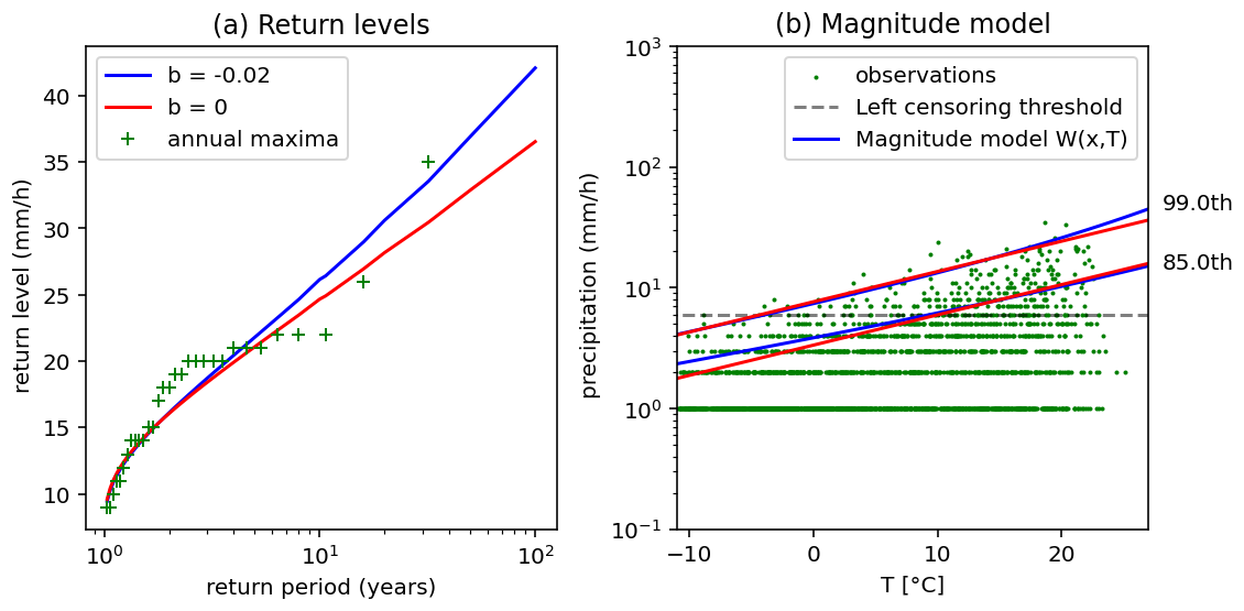
Figure 1 Example to show the impact the shape parameter has on tail heaviness and the resulting return levels from a station in north Japan (45.25, 141.85). Panel (a) shows the return levels, with shape parameter dependence on temperature in blue. No dependence on temperature in the shape parameter is in red. Panel (b) shows the magnitude model, i.e. the relationship between temperature and extreme precipitation.

These contrasting results lead to the question of whether a dependence of the shape parameter on temperature should be included when using this type of model. If there is a dependence, there are three main options for dealing with the parameter that defines the dependence: it can be allowed to vary freely at a particular station, it can be set to a reasonable value based on prior knowledge of the climatology of the region, or it can be neglected (although it exists).

Here, we investigate how the temperature dependence can be estimated from observed records without introducing large errors and uncertainty. Specifically, we answer the following questions: (i) does the shape parameter exhibit a significant dependence on temperature in different regions of the world? If there is a dependence, how does its direction and magnitude vary in space?; (ii) how much of the observed variation in such dependence can be attributed to spatial variability rather than sampling uncertainty?; (iii) does including this dependence influence the time-invariance assumption behind these approaches?; and (iv) does this dependence affect the estimates of return levels? How is this affected by the length of the data record? We conclude by giving some practical recommendations for when and if a dependence of the shape parameter of the Weibull magnitude model should be included in the TENAX-like frameworks.

2 The TENAX model

A full description of TENAX can be found in Marra et al. (2024). Here, we summarise the basics necessary for this paper. First, independent precipitation events are identified. These are defined as the peak precipitation intensities observed over the duration of interest, in our case, 1 h, during an independent storm. To ensure independence, storms are required to be separated by a minimum of 24 dry hours. The temperature value T assigned to an event is the temperature averaged in the 24 h preceding the event. TENAX includes a temperature model g(T), which quantifies the probability of having a precipitation event at a given temperature, and a magnitude model W(x;T), which quantifies the exceedance probability of heavy precipitation magnitudes for events at a given temperature.

For the temperature model, we use a generalised normal distribution with shape parameter β=4:

$$\begin{array}{}\text{(1)}& g\left(T\right)={\displaystyle \frac{\mathrm{2}}{\mathit{\sigma }\mathrm{\Gamma }\left(\frac{\mathrm{1}}{\mathit{\beta }}\right)}}\exp \left[-{\left({\displaystyle \frac{T-\mathit{\mu }}{\mathit{\sigma }}}\right)}^{\mathit{\beta }}\right].\end{array}$$

The location parameter μ and the scale parameter σ are estimated using the maximum likelihood method.

TENAX's magnitude model is a non-stationary Weibull distribution, with temperature as the covariate. A Weibull distribution was chosen because this should approximate the tail of heavy precipitation based on atmospheric physics arguments (Wilson and Toumi, 2005). It is given by:

$$\begin{array}{}\text{(2)}& W(x;T)=\mathrm{1}-\exp \left(-{\left[{\displaystyle \frac{x}{\mathit{\lambda }\left(T\right)}}\right]}^{\mathit{\kappa }\left(T\right)}\right),\end{array}$$

where λ(T) is the scale parameter and κ(T) is the shape parameter. Since extreme precipitation is expected to scale exponentially with temperature following the Clausius-Clapeyron relationship (Fowler et al., 2021), an exponential dependence on temperature T is used in the scale parameter: λ(T)=λ₀e^aT. The shape parameter affects the tail-heaviness of the Weibull distribution, and previous observational studies have suggested that this might also have a dependence on temperature (Lenderink and van Meijgaard, 2008; Hardwick Jones et al., 2010). We investigate both a linear and exponential dependence in the shape parameter, namely $\mathit{\kappa }\left(T\right)={\mathit{\kappa }}_{\mathrm{0}}+bT$ or $\mathit{\kappa }\left(T\right)={\mathit{\kappa }}_{\mathrm{0}}{e}^{b_{\exp }T}$. In principle, the linear dependence raises the possibility of a negative shape parameter if temperatures change considerably. However, our analyses showed that temperature changes are not large enough for this to become an issue in real cases. More in general, the exponential dependence prevents this from happening. The parameters in the magnitude model are estimated by left-censoring the values below the 90th percentile of the events, meaning that the values below this threshold are retained for the estimation and treated as non-exceedances (see Marra et al., 2020), using a maximum likelihood estimator.

The combination of the magnitude model W(x;T) and the temperature model g(T) using the total probability theorem gives the cumulative distribution function of the event magnitudes:

$$\begin{array}{}\text{(3)}& F\left(x\right)=\underset{\mathrm{0}}{\overset{\mathrm{\infty }}{\int }}W(x;T)\cdot g\left(T\right)\mathrm{d}T.\end{array}$$

The cumulative distribution function of the annual maxima emerging from independent samples is then given by G(x)=F(x)ⁿ, where n is the average number of events per year (Marra et al., 2020). Since this integral doesn't have a practical closed-form solution, we use a Monte Carlo approximation with $N=\mathrm{2}\times {\mathrm{10}}^{\mathrm{5}}$ iterations to approximate Eq. (3). Hence,

$$\begin{array}{}\text{(4)}& G_{\mathrm{TENAX}}\left(x\right)={\left({\displaystyle \frac{\mathrm{1}}{N}}\sum _{i=\mathrm{1}}^{N}W(x;T_i)\right)}^n,\end{array}$$

where T_i are temperatures sampled from g(T). Return levels are calculated by inverting Eq. (4) numerically.

3 Precipitation and temperature data

Hourly precipitation data were taken from the global sub-daily rainfall (GSDR) dataset (Lewis et al., 2019a). The data lengths vary greatly. For our initial spatial analysis (see Sect. 4), we used stations with at least 10 years of complete data, where a complete year is defined as one with less than 10 % missing data. When investigating hindcasts, we only used stations with at least 20 complete years. We focused our analysis on the four countries with the highest number of stations meeting the 10-year completeness criterion: the UK (913 stations), the USA (1365), Germany (696), and Japan (1207).

Hourly temperature data were obtained from the ERA5-land reanalysis dataset (Muñoz-Sabater et al., 2021). The ERA5-land grid cell closest to the coordinates of each station was chosen. The majority (94 %) of stations had temperature data within the same grid cell. A few stations, such as those on small islands or very close to the coast were not directly within a land grid cell. The average distance between the coordinates of a station and the ERA5-land cell was 4 km. If there were no grid cells with data within 0.5° distance of a station, the station was not used in our analysis.

4 Analysis

First, we calculated the parameters of the TENAX model at each station with more than 10 years of complete data using maximum likelihood estimation and a likelihood ratio test to check whether b was significantly different from 0 at the 5 % significance level. The parameters were estimated three times: for both the linear and exponential formulation of the model (“free b”) and for the case when b was set to zero (“b=0”).

The parameters of the TENAX model are estimated from a finite set of events, and as such, there is a stochastic uncertainty caused by the limited sample size. To investigate the stochastic uncertainty and its relation to b, we performed Monte Carlo simulations. For each station in a country, we simulated precipitation and temperature events equal to the number of observed events at that station. We used the average observed parameters over the country and repeated this with b=0 and with b allowed to vary. From these simulated events, we recalculated the parameters, repeating this process five times to reduce sampling uncertainty and obtain robust distributions. Five is an arbitrary number which was chosen as a balance between computation time and stability of the results. The distribution of these parameters represents the expected stochastic spread due to sampling uncertainty. For a summary of the values used to produce the Monte Carlo simulations, see Table S1 in the Supplement. To directly compare the spread of the generated and observed parameters, we calculated the ratio of the interquartile ranges.

As per TENAX's assumptions, the parameters of the magnitude model are required to be time-invariant. This is motivated by the idea that the magnitude model represents the physical relationship between temperature and extreme precipitation which is not expected to change with climate change. We investigated the effects of b on this time invariance in a hindcast setup. We split the time series at each station in half and computed the parameters of the magnitude model in each half separately. To compare each parameter between the two time periods, we calculated the root mean square difference and the Pearson's correlation coefficient in space. We also compare the magnitude model as a whole by using a likelihood ratio test to see if the model is significantly different between the two periods (see Marra et al., 2024, Sect. 3.2, for more details on this test).

Finally, we used Monte Carlo simulations to understand the impact of b on the accuracy of the estimated return levels. We did this by choosing three representative values of b: −0.015, 0, and 0.015 °C⁻¹, and typical values for the other parameters: a=0.07 °C⁻¹, λ₀=1 mm h⁻¹, κ₀=1.1, μ=10 °C, and σ=13 °C. We created synthetic data sets of precipitation and temperature events, assuming 80 events per year for 10-, 20-, and 30-year record lengths. From the synthetic data, we estimated the parameters with three different techniques: letting b be fitted (“free”), and setting b to the value used to generate (“set”), therefore mimicking a situation in which b is known (for example, in virtue of the local climatology), and setting b=0. We then compared the return levels resulting from these different estimates with the “true” return levels obtained from the original generating parameters. This is repeated 1000 times to get a range of the possible return levels a single distribution can generate using different techniques. We calculated the “multiplicative bias in return levels” as the ratio of the recalculated return levels to the expected return levels.

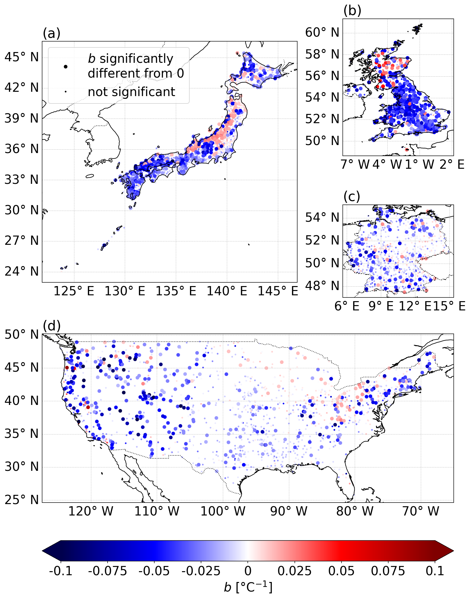
Figure 2 The values of the temperature coefficient in the shape parameter b calculated at stations in (a) Japan, (b) the UK, (c) Germany, and (d) the USA. Larger points are the stations where b is significantly different from zero at 5 % significance.

5 Results

5.1 Significant dependence on temperature in the tail heaviness

The significant dependence of the shape parameter on temperature across different regions of the world is presented in Fig. 2 for the linear formulation of b. Results for the exponential formulation, which show similar patterns, are provided in Fig. S1 in the Supplement and are not discussed. The b parameter is significantly different from zero (p value of 5 %) in 36 % of stations in Japan, 44 % of stations in the UK, 14 % of stations in Germany, and 28 % of stations in the USA. The majority of significant b values, as well as their average value, are negative in all regions, meaning that the temperature-precipitation scaling of rarer extremes tends to be higher than that of milder extremes. We should note that these statistics are not completely reliable since the stations are unlikely to be completely independent which brings issues of multiple hypothesis testing.

In Germany, the locations of stations with significant b are randomly distributed, as is the magnitude of b (Fig. 2c). Despite the random distribution of b in Germany, a one-sample Student's t test shows that the average value of b is significantly different from zero at 1 % significance level, pointing to an average value (standard deviation) of −0.012 °C⁻¹ (0.017 °C⁻¹) for the country. In contrast, Japan, the USA, and the UK show a spatial pattern in the size and magnitude of b. In Japan (Fig. 2a), significant negative values are clustered mainly in the southern half of the country, along the central ridge, and in the northernmost part of the country. Significant positive b values are clustered in north-central Japan. The average value of b throughout all Japan is −0.013°C⁻¹ (0.022 °C⁻¹). In the central and south USA (Fig. 2d), between approximately 105W and 95° W, b in the majority of stations (85 %) is not significantly different from zero. However, further west of 105° W, only 51 % of the b values are not significant. Of the significant values in that region, 94 % are negative. In the north-west, there is a mixture of positive and negative significant b values. Focussing on the region east of 95° W and north of 38° N, we find that 74 % of stations here have non-significant b. Of those that are significant, 62.5 % are negative, a lower value than in other regions. The average of all b values in the USA is −0.015 °C⁻¹ (0.024 °C⁻¹). In the UK (Fig. 2b), positive values of b are more likely to be found north of 55° N. However, the average in this region is still negative: −0.012 °C⁻¹ (0.032 °C⁻¹). South of here, the majority of values are negative, with an average value of −0.027 °C⁻¹ (0.022 °C⁻¹). The average value of b in the entire UK is −0.024 °C⁻¹ (0.025 °C⁻¹). Overall, b is significantly different from zero in many locations, and exhibits some regional dependence. It seems to be linked to a range of factors, including latitude, elevation, climatic conditions, and prevalent synoptic forcing.

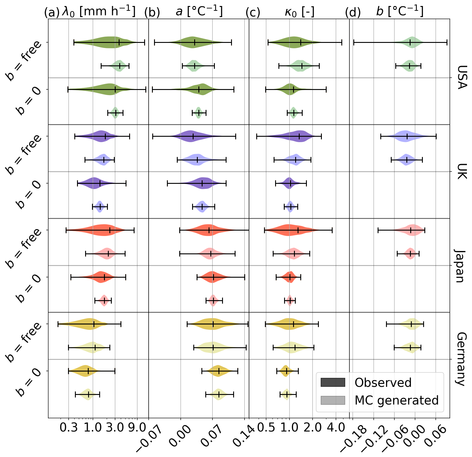
Figure 3 Distribution of parameters of the magnitude model in the USA (green), UK (blue), Japan (red), and Germany (yellow). The darker plots are the observed values, and the lighter plots are the Monte Carlo generated values. In each country, the upper two plots are the parameters when b is fitted freely, and the lower two plots are the parameters when b=0. Vertical lines are the minima, mean, and maxima.

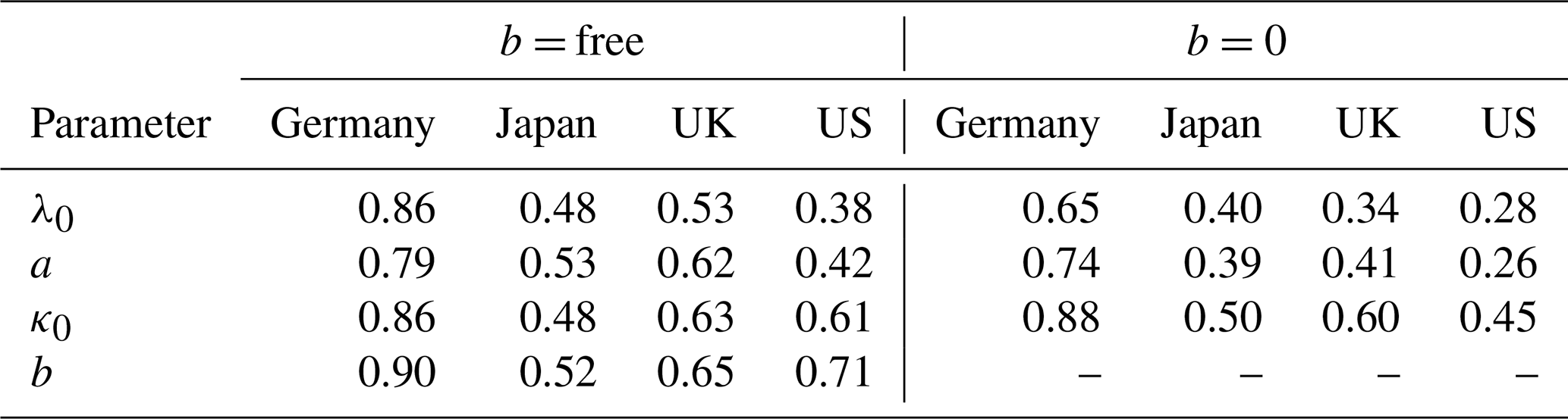
Table 1 The ratio of the interquartile range of the generated parameters to the interquartile range of the observed parameters in each country.

5.2 Disentangling stochastic uncertainty and spatial variability

Violin plots of the parameter estimates for both the observed and Monte Carlo generated parameters are presented in Fig. 3 for the linear b formulation (and in Fig. S2 for the exponential formulation). All four regions and all parameters have a smaller spread in the generated parameters than in the observed ones, so not all the variation in the observations can be explained by stochastic uncertainty alone. Table 1 shows the ratios of the interquartile range between the generated and observed values (Table S2 presents the ratios for the exponential case). A larger value means a greater proportion of the spread can be explained stochastically. For b, the country with the most spatial variation is Japan. Germany has the least spatial variation, as expected from the number of significant values discussed in Sect. 5.1. The other parameters, λ₀, a, and κ₀, also present a larger range of values than expected from stochastic variability alone in all the regions. In general, there is not much consistency between the countries in which the parameter has the largest amount of variation.

Note that there are 5 times as many simulated parameters as observed parameters. This does not affect the interquartile ranges, but does mean we are more likely to see very large or small values. Hence, some of the simulated violin plots in Fig. 3 appear to have a greater range than the observed ones. The increase in outliers shows that the number of events at a station affects the uncertainty in estimating the parameters. For experiments run without these 5 repeats, see Figs. S3 and S4 and Tables S3 and S4.

Comparing the free b with the b set to zero scenarios (Fig. 3), we spot a reduction in the spread in the values both in the observations and in the Monte Carlo generated samples. When b=0, the parameter a is the scaling rate between extreme hourly precipitation and temperature, expected to be close to 0.07 °C⁻¹. On average, this is approximately the case for Japan and Germany. When b is introduced (i.e., non-zero), the average values of a shift to lower values (which means weaker scaling rates) to accommodate the negative b (which means stronger scaling at rarer probabilities). For example, in Japan, the average value of a is reduced from 0.072 °C⁻¹ in the case of b equal to zero to 0.062 °C⁻¹ when b is free.

When b=0, the ratio is reduced for almost all parameters and locations (Table 1). This means that a larger amount of the variability is due to genuine variation, rather than stochasticity. This is because including the additional parameter b inflates the parameter estimation uncertainty, while the spatial variability changes less. Overall, the distribution of b in Germany can largely be attributed to stochasticity, while in other countries there is a large amount of spatial variability. Including b as an unknown parameter which needs to be estimated, however, largely increases the stochastic spread of the other parameters.

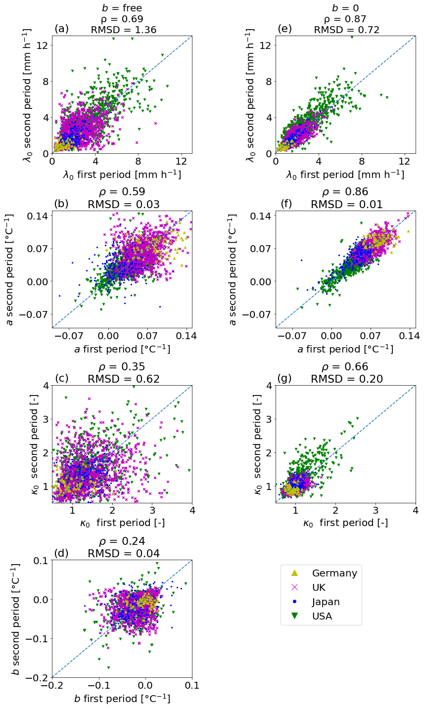
Figure 4 Scatter plots of the parameters in the magnitude model when the time series is split in half (hindcast mode). Left column (a–d) is for b = free and right column (e–g) is for b=0. Colours represent the country the station is in, and the one-to-one line is plotted in blue dashes.

5.3 Time-invariance of the magnitude model

Figure 4 presents scatter plots of the parameters of the magnitude model W(x;T) in hindcast mode, i.e., by splitting the data for each station into two periods. In general, all parameters follow the one-to-one line with some outliers. When b=0, all the parameters follow the line more closely and the correlations increase, especially for the parameter κ₀, which is strongly influenced by b.

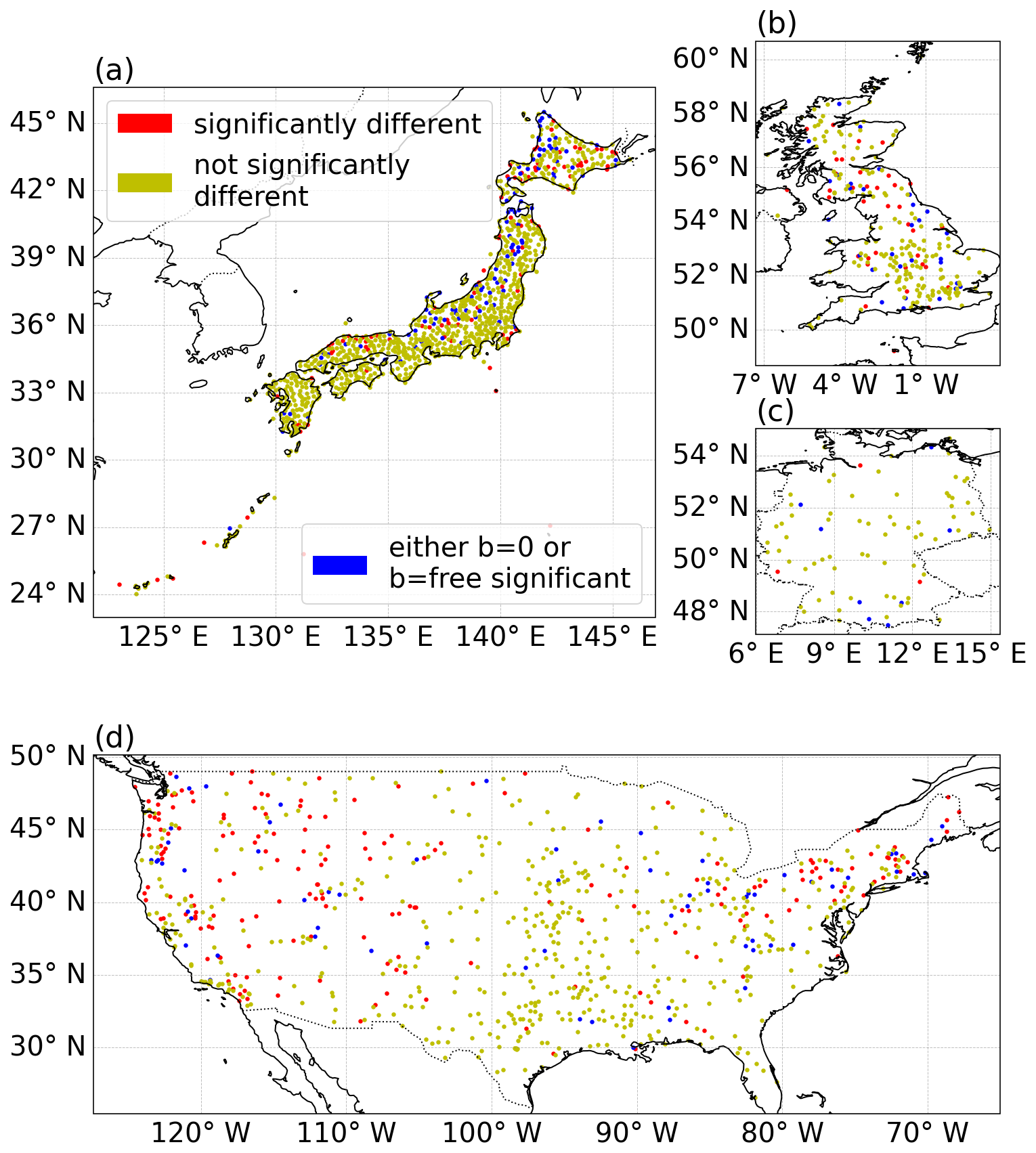
Figure 5 Maps showing where differences in the magnitude models are significant (red) or not significant (yellow), regardless of whether b is fixed to zero or allowed to vary freely. Blue points are locations where the magnitude model for all parameters is significantly different between the two time periods either for b=0 OR b= free (but not both).

The time invariance of the magnitude model as a whole can be assessed by testing if the model produces significantly different results when applied to the two periods separately compared with the entire time series. We do this with a likelihood ratio test. We look at two cases: b set to zero and b allowed to vary. Figure 5 shows which stations have significantly different magnitude models at 5 % significance when b is included or set to zero. In all countries, the majority of stations do not display significant differences in both cases (66 % to 86 % of stations). The USA has the largest proportion of stations that have significantly different magnitude models. Of these, 75 % are significant regardless of whether b is included. Slightly more stations (4.4 %) are significant when b is included than not (4.2 %). Germany is also inconclusive, with the same number of stations being significant in one case as in the other. However, in the UK and Japan, the number of stations that have significant differences when b is included but not when b=0 was over double the amount in the opposite case. It is therefore difficult to understand the extent to which including b affects the hindcast significance. However, the scatter plots and correlation coefficients show that freely estimating b from the observations largely increases the variability in the other parameters between the two time periods, as a consequence of the increased stochastic uncertainty.

Using the exponential instead of the linear dependence in the shape parameter produces similar correlations for λ₀, a, and b_exp but reduces the correlation in κ₀ by a substantial amount (Fig. S5). This is in part due to the presence of large outliers. In fact, the exponential dependence has a dampening effect on the potential magnitude of precipitation. It appears that in some cases, this causes the parameters to over-compensate in the model, leading to unreasonable values.

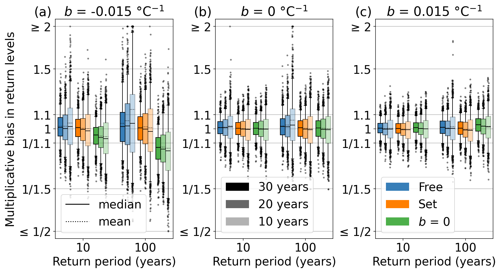
Figure 6 The bias in synthetic return levels for different values of b. The whiskers of the box plots are the 5th–95th percentiles. Bar colours represent b setup as allowed to vary (blue), set to its actual value (orange), or set to 0 (green). Bars' opacity represents the record length generated by the model (30-, 20-, and 10-year).

5.4 Impact on return level estimates

To assess the potential influence of b on the estimates of rainfall return levels, we present the ratio between return levels derived using the model in different setups and the “true” return levels obtained from the known synthetic parameters (Fig. 6). Note that these are completely synthetic. We chose λ₀, a, κ₀, b, μ, σ and n to be representative of the typical observed values. When b is negative (Fig. 6a), the variation in return levels is the highest. Allowing b to be fitted and setting b to the known value produce results that are, on average and as expected, the closest to the actual return level, while setting b to zero underestimates the return levels, especially at higher return periods. This, along with the fact that our observed values of b are usually negative, show that ignoring trends in the shape parameter risks underestimating return levels. When shorter record lengths are used to estimate b, however, the error increases vastly, especially for higher return periods, and fitting b results in unrealistically large return levels. The mean values of the estimated return levels when b is fitted are larger than the median, implying positive skew. The linear and exponential treatments of b have similar patterns, but the variation in the exponential distributions is smaller, and there are fewer large outliers leading to overestimation of return levels (Fig. S6).

When generating a scenario in which b is zero (Fig. 6b), letting b vary in the model (blue) leads to overestimation of return levels. This is more pronounced at higher return periods and with shorter data lengths. In this case, “Set” and “b=0” are equivalent. All methods produce an average value that is close to the expected return level, but fitting b produces more outliers, especially ones that overestimate the return levels.

When b is positive (Fig. 6c), the variation in estimated return levels is smaller, likely because the return levels themselves are lower. Still, letting b be free results in larger outliers than the other methods, especially with shorter record lengths and at high return periods. Using b=0 in this case leads to overestimation of return levels, but not to the same extent as the underestimation for negative b. Since the observed values of b are more commonly negative than positive, the main concern should be with the potential of underestimation if b=0 than this overestimation.

6 Discussion

We find that the shape parameter in TENAX shows a statistically significant dependence on temperature in many locations. The typical value of this dependence (negative b parameter, Fig. 1) indicates that the temperature-precipitation scaling of rarer extremes tends to be higher than that of milder extremes. Including this negative b will lead to larger estimated return levels, especially at longer return periods (Fig. 6). It would be beneficial for future work to further explore in detail the physical reasons for the spatial variability of the b parameter. It could be linked to, for example, orography, elevation, or large-scale dynamical drivers. A Bayesian framework for calculating b, and the parameters of TENAX more generally, would also help to understand and reduce uncertainty.

Andria et al. (2025) suggest that this dependence should be exponential. We find that the difference between exponential and linear dependence is small, although the exponential dependence seems to cause larger uncertainties in the other parameters of the model. In this concern, it should be noted that Andria et al. (2025) use a different statistical setup, in which temperature bins are identified and several parameter sets are estimated without resorting to left censoring. The dependence of the shape parameter on temperature is then assessed ex post. Hardwick Jones et al. (2010) found that the observed scaling in east Australia increased by about 50 % between the 75th and the 99th percentile. For the average values of the parameters in Japan, we find an increase of about 20 % between these two percentiles. In the USA, the scaling rates are smaller, but with the average values, we also find an increase of 50 % between the 75th and 99th percentile.

The apparent dependence of b on location and orography implies that it is accounting in some way for the dynamical changes associated with temperature changes. For example, in some locations, climate change is associated with more intense circulation patterns in convective precipitation and shifts from stratiform to convective regimes, and super Clausius–Clapeyron scaling is observed (Da Silva and Haerter, 2025). Hence, using only the b parameter to represent a vast array of precipitation mechanisms in some locations may be an oversimplification.

We note that some stations in the GSDR dataset had a change in the sampling resolution of precipitation during the observation period. For example, the resolution of some records changed from 2.54 to 0.254 mm h⁻¹. This may affect the calculations of the parameters and the hindcasts. We re-run our analyses excluding all these stations, but no differences in the results could be noticed. Removing stations with less than 20 years of available observations from the hindcasts was more effective in reducing the presence of extreme outliers. This seems to indicate that the data length is more important to the quality of the results than consistency in resolution.

To match temperature values to precipitation, we used a reanalysis dataset. This may not align with the actual near-surface air temperature that one would measure using ground observations, especially on the scale of individual stations. Mistry et al. (2022) found that there was a high correlation between the observed daily temperatures at stations and the temperatures produced by ERA5-land, especially in the countries we investigate. Although Sheridan et al. (2020) found that ERA5 was better than ERA5-land at representing extreme heat events, we chose to use ERA5-land for its finer resolution. Other products, such as regional ones, may give more accurate temperatures, but would not allow us to compare study areas across the globe. In any case, temperatures are averaged over the 24 h preceding each event, limiting the potential impact of misrepresenting the location of small-scale weather events in ERA5-land. When producing the stochastic simulations of the parameters, we used the temperature model given in Eq. (1). In some locations, this may not give an accurate range of temperature values. Given infinite events, the magnitude model and temperature model are independent, so the temperature model used would not affect the parameters of the magnitude model. However, within a finite sample, the limited temperature values may affect the magnitude model.

Practical recommendations

While the spatial variability observed in b cannot be attributed solely to stochastic uncertainty, the stochastic component is of the same order of magnitude as the spatial variability (Fig. 2). This contrasting behaviour brings the fundamental question of whether the dependence should be allowed in practical applications.

When producing models for extreme rainfall with temperature as a covariate, we recommend checking if there is a temperature dependence in the shape parameter and investigating its behaviour when using an exponential and linear dependence. Excluding b will often lead to underestimation of the return levels, especially at longer return periods. In contrast, leaving b to be freely estimated from the (usually limited) observations is associated with large uncertainty, leading to noisy estimates and, often, to unrealistic estimates of the return levels. Developing some prior knowledge about b in a region of interest can largely improve our estimates. In particular, setting b to a chosen, realistic non-zero value seems a good compromise. If there are enough stations with sufficiently long measurements in a region of interest, b can be set to the average calculated value of b in the region, following methods such as in Kjeldsen and Prosdocimi (2021) or Renard et al. (2006). If this is not possible, setting b=0 remains the recommended option, with the awareness that larger return levels might be underestimated.

7 Conclusions

We investigated the dependence of heavy hourly precipitation tail heaviness on temperature using the framework provided by the TENAX model (Marra et al., 2024) for multiple stations worldwide. We found that in many of the stations the shape parameter of the distribution exhibits a significant dependence on temperature (b≠0). The sign and size of this dependence present a spatial pattern and appear to be linked to latitude, elevation, climatic conditions, and large-scale drivers. Future work could investigate these influences specifically. Monte Carlo simulations show that, aside from Germany, the variation within the countries investigated is not attributable to stochastic uncertainty alone. Including b in the magnitude model increases the variability in the other parameters of the magnitude model, but does not make a large difference to whether the magnitude model is invariant in time when performing hindcasts. Calculating b from data at a single station may lead to a large over-estimation of return levels, especially for stations with shorter record lengths. Using an exponential dependence rather than a linear one somewhat mitigates against this, but yields larger uncertainties in the remaining model parameters.

With these conclusions in mind, we recommend the following. If only short record lengths are available (between 10 and 20 years), b should not be estimated from the individual stations alone, since the uncertainty introduced may severely bias the estimation of the return levels and of the other parameters in the magnitude model, leading to inconsistent projections. At the same time, b should not be neglected completely, since it is certainly non-zero in many regions, and its exclusion leads to an underestimation of return levels. Having prior knowledge about this dependence would largely improve the estimates. In ideal conditions, b should be estimated in the context of surrounding stations, with care to ensure the values are physically reasonable. Setting b to a reasonable, well-supported, non-zero value, such as the average value within an adequately identified region, would be a viable option to reduce these uncertainties while retaining the physical meaning of this parameter. When no prior information on b is available, setting it to zero remains the recommended option.