Metrics that matter: objective functions and their impact on signature representation in conceptual hydrological models

Although objective functions (OFs) are widely discussed in the literature, many modelling studies still default to a few common metrics, without much consideration of their relative strengths and weaknesses. This paper systematically investigates the impact of OF choice on the representation of various streamflow characteristics across 47 conceptual models and 10 hydro-climatically diverse catchments selected from the CARAVAN dataset. We use eight different OFs for calibration, including the Kling–Gupta efficiency (KGE), Nash–Sutcliffe efficiency (NSE), a variant of each that uses a streamflow transformation, and four more recently proposed metrics. We further account for parameter uncertainty by retaining the top 500 parameter sets for each combination of model, basin and OF. We evaluate the representation of 15 hydrological signatures that capture a relevant selection of streamflow characteristics to determine generalisable strengths and weaknesses of individual OFs across different models and hydroclimatic conditions. A random forest importance analysis showed that OF choice is often more influential than model structure choice in determining signature representation, with catchment characteristics remaining the dominant control. While certain signatures, particularly those related to flow variability, are relatively insensitive to OF choice, other signatures exhibit large performance shifts across different OFs. As other studies have already noted, no single OF performs best across all signatures. Our consistent multi-model and multi-catchment experiment now provides generalisable guidance on which OF best reproduces which aspect of streamflow behaviour. This helps to better select objective functions most appropriate for a specific modelling purpose and provides insights into which metric combinations can cover a broader range of flow characteristics.

1 Introduction

Setting up and running a hydrological model requires modellers to make many decisions. These may include the choice of a suitable model (structure), sensible parameter boundaries, an appropriate calibration period, and which method to use for forcing data interpolation. Selecting which performance metric(s) to employ as the objective function during model calibration is another critical decision where research has shown that different performance metrics can lead to substantially different model outcomes. Mai (2023), for example, tested six alternative calibration metrics and found marked differences in the resulting hydrographs. Garcia et al. (2017) compared variants of the KGE metric for low-flow simulation, observing large differences in annual runoff estimates. Studies such as Pool et al. (2017) and Vis et al. (2015) further demonstrated that the choice of performance metric for calibration influences how well the model reproduces key hydrological signatures (i.e., streamflow characteristics). Similarly, Mendoza et al. (2016) and Seiller et al. (2017) show the impact calibration choices can have on the portrayal of climate change impacts.

The choice of calibration metric, therefore, plays a crucial role among the various decisions involved in model calibration, evaluation, and diagnostic analysis. It directly determines how model parameters are optimized and, consequently, how well the resulting simulations reproduce both observed data and underlying hydrological processes. Despite the well-established influence of objective function selection, and an extensive body of research discussing the individual strengths and weaknesses of various performance metrics (e.g. Thirel et al., 2024; Althoff and Rodrigues, 2021; Cinkus et al., 2023; Knoben et al., 2019b; Mizukami et al., 2019; Bennett et al., 2013; Gupta et al., 2009; Krause et al., 2005), Jackson et al. (2019) conclude that: “in most hydrologic modelling studies error metrics are chosen based on familiarity, [and] without consideration of the relative strengths and weaknesses” in their review of more than 60 different performance metrics. And indeed, a quick and informal review of 60 modelling studies in the existing literature library of the authors supports this claim by showing that most studies provide little to no reasoning for their choice of objective function (Fig. 1; details on review in the Supplement). The papers that gave reasoning mainly referred to general characteristics and perceptions of their metric of choice. Reasons we documented (see Supplement) can roughly be classified into various forms of “the KGE is a more balanced metric than the NSE”, “NSE is a common metric for high flows”, “logNSE/logKGE focus on low flows”, “NSE/KGE are widely used metrics” or “we use this metric because it is comparable with previous studies”.

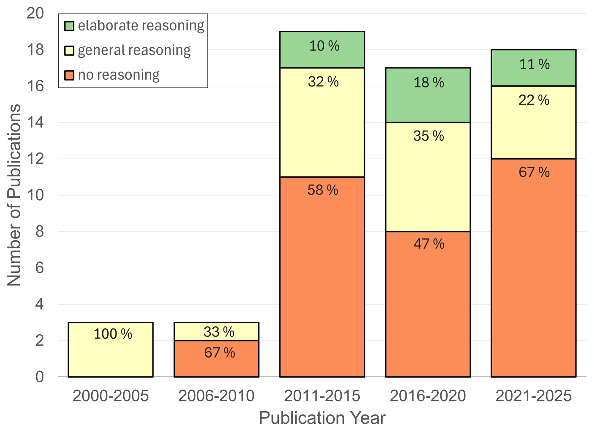
Figure 1 Number of analysed studies published during different five-year periods and the percentage of these studies that give no – general – or elaborate reasoning on their choice of objective function. This data stems from an informal/non-exhaustive literature review of 60 studies taken from the authors' literature database. Details regarding the review are given in Supplement.

We believe that part of the prevailing tendency to define objective functions in an often ad-hoc manner is the broad but scattered and often site- and/or model-specific research on the impacts of different performance metrics used as objective functions. Most good modelling practice guidelines (e.g. van Waveren et al., 1999; Jakeman et al., 2006, 2018) simply advise to select an appropriate objective function that aligns with the purpose of the modelling study, but do not provide guidance on how to do so. The question of how to connect the choice for a suitable calibration metric to a specific modelling purpose thus remains unclear (Jacobs et al., 2024). While several studies have investigated connections between objective function choice and how the calibrated models represent certain streamflow characteristics, they are often limited in the number of models they use (1 model in e.g. Hallouin et al., 2020; Melsen et al., 2019; Pool et al., 2017; Vis et al., 2015) or signatures they consider (less than 5 in e.g. Araya et al., 2023; Mizukami et al., 2019; Seiller et al., 2017). As Table 1 highlights, studies with a similar focus to our study also mostly consider catchments of only one specific region or country and no study the authors are aware of tested more than 12 models while also considering several metrics and signatures.

Althoff and Rodrigues (2021)Araya et al. (2023)Hallouin et al. (2020)Hernandez-Suarez et al. (2018)Melsen et al. (2019)Mendoza et al. (2016)Mizukami et al. (2019)Pool et al. (2017)Seiller et al. (2017)Vis et al. (2015)

Table 1 Summary of similar studies that investigate the impact of objective function choice on the representation of hydrological signatures. We compare the number of investigated models, catchments, metrics and signatures to this study. Note that studies with an ^* asterisk also tested combinations of different metrics (i.e. composite criteria or multi-metric objective functions) in addition to individual calibration metrics.

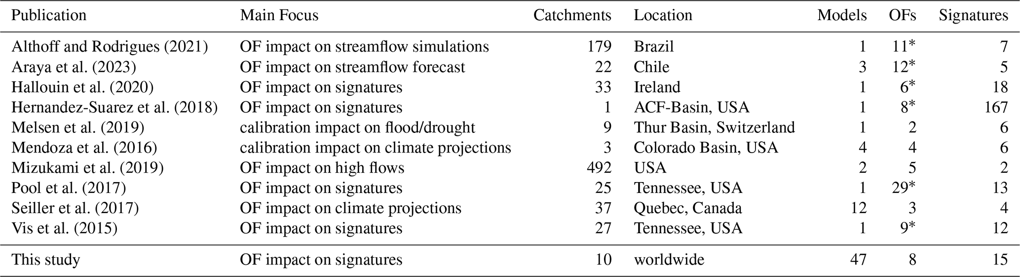
Some of the existing studies show recurring tendencies across regions and models. For instance, Pool et al. (2017) and Hallouin et al. (2020) found that traditional objective functions such as NSE or KGE can perform as well or better than tailored signature-based metrics for predicting flow characteristics not explicitly included in calibration. Mizukami et al. (2019) similarly noted that application-specific metrics may excel at their target but can degrade performance on other metrics. Generally, most studies can identify a preferred metric or metric combination. However, that selection is strongly conditioned to the modelling purpose, the flow conditions of interest, and the hydroclimatic setting of the individual study (e.g. seasonal forecasting in snow-influenced catchments for Araya et al. (2023) or tropical low-flow applications for Althoff and Rodrigues (2021)). A robust transfer of findings to new contexts is therefore difficult and further complicated by inconsistent experimental designs across studies (differing catchment sets, model selections, and signature choices), which prevent a straightforward synthesis on how metric choices influence signature representation.

To address this problem, this study aims to develop a more generalised understanding of how the choice of performance metric used for model calibration influences the representation of the hydrological behaviour. We focus on single-objective calibration because it remains the calibration standard and can provide insights into metric combinations that might serve as complementary multi-objective calibration targets. By systematically analysing catchments that span a broad range of climatic conditions and employing a large set of conceptual model structures, we seek to identify general benefits and limitations associated with different calibration metrics across diverse hydrological contexts. The selected set of catchments, though limited in number, was chosen based on differing climate indices (moisture, seasonality, and fraction of snow), to ensure a representative spread of hydroclimatic conditions. This enables us to examine how models calibrated with different performance metrics behave under varying hydrological regimes while also balancing depth with breadth of analysis (Gupta et al., 2014). We evaluate how 47 conceptual model structures, each calibrated using alternative performance metrics and an ensemble of high-performing parameter sets to account for parameter uncertainty, reproduce 15 selected hydrological signatures that describe distinct aspects of the flow regime, such as flow variability, baseflow contribution, and runoff dynamics. This multi-dimensional setup contributes to identifying generalisable strengths and weaknesses of individual performance metrics that extend beyond their known sensitivities to particular flow conditions, offering new insights into how calibration choices influence process realism in conceptual hydrological modelling. The following sections will introduce the catchments, models and signatures we used (Sect. 2), present the results (Sect. 3) and provide an overarching discussion of the implications metric choice can have on the representation of the hydrological behaviour as well as limitations and future steps (Sect. 4). Conclusions are presented in Sect. 5.

2 Methodology

Figure 2 gives an overview of the methodology used in this study. We calibrate 47 conceptual hydrological models from the Modular Assessment of Rainfall–Runoff Models Toolbox (MARRMoT) (Knoben et al., 2019a; Trotter et al., 2022) using eight different calibration metrics. The models and metrics used are introduced in Sect. 2.1.1 and 2.1.2 respectively. We calibrate all of these models (as described in Sect. 2.2) for a subset of 10 hydro-climatically differing catchments from the CARAVAN dataset (Kratzert et al., 2023) as introduced in Sect. 2.1.3. For each calibration run, we retain the top 500 parameter sets for further investigation. After selecting only the well-performing model structures according to a benchmark procedure (Sect. 2.3) we use the simulated discharge timeseries to calculate 15 selected signatures that represent varying aspects of the hydrological behaviour (as introduced in Sect. 2.4). Through a comparison of the simulated and observed signature values we are able to identify the strengths and weaknesses of the tested metrics in representing the hydrological regime over a broad range of hydro-climatic conditions and different model complexities.

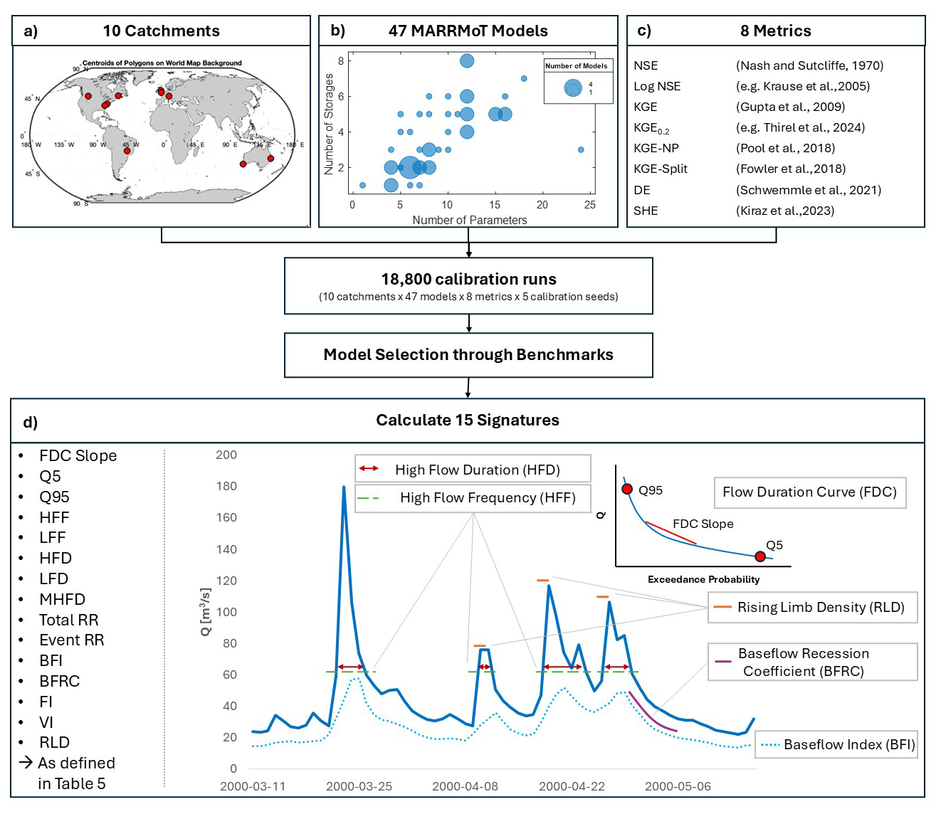
Figure 2 Overview of the experiment design of this study. (a) Shows the geographical location of the study catchments. (b) Visualizes the different complexities (number of storages vs number of parameters) of the investigated MARRMoT Models. (c) Lists the eight objective functions used for calibration. (d) Lists the 15 hydrological signatures investigated and shows a schematic visualization of some of them.

2.1 Experiment Components

2.1.1 Models

We obtained the 47 models used in this study from the MARRMoT toolbox (Knoben et al., 2019a; Trotter and Knoben, 2022), because the toolbox allows easy and consistent use of the different models. These models are based on the scientific literature and mimic some widely used and well-known models such as HBV, GR4J, TOPMODEL, VIC and HYMOD. A full list of all models included in this analysis can be found in the Supplement. Of note, only 12 of the 47 models possess a snow module. Details of these modules vary depending on the model under consideration. Figure 2b shows how the model structures differ in their number of considered stores (i.e., state variables) and parameters and therefore gives an idea of the different models' complexity. The number of parameters ranges from one to 24 and the number of considered stores ranges from one to eight. The simplest model has one store and one parameter, whereas the most complex models have eight stores and 12 parameters, or three stores and 24 parameters. By using such a wide range of different complexities in model structures, we ensure that the strengths and weaknesses identified generalise across different model structures.

2.1.2 Objective Functions

We calibrate the 47 hydrological models with eight objective functions, each based on a different performance metric, and analyse how well the calibrated models simulate 15 streamflow signatures. We differentiate between model accuracy, expressed by the objective function value, and model adequacy, expressed by signature representation. This selection of eight metrics is necessarily non-exhaustive, many further metrics and transformations exist, but was chosen to span widely used and recently proposed formulations while keeping the analysis tractable. In general, performance metrics are numerical measures used to quantify model performance, whereas objective functions refer to the use of such metrics as optimization targets during model calibration. We therefore use “objective function” or “OF” when referring to their role in calibration, and “metric” when referring to their mathematical formulation or diagnostic properties. To describe them, we introduce the following set of common symbols: Q and P denote streamflow and precipitation respectively. σ and r are standard deviation and correlation. Subscripts are used to indicate the specifics of all mentioned variables, e.g. Q_s and Q_o show simulated and observed streamflow respectively. Subscript t refers to individual time steps. For correlation, the subscripts r_pe and r_sp are used for Pearson and Spearman correlation. Overlines are used to indicate temporal means. In sums, the letter n is used to indicate the total length of the time series.

Table 2 Equations of the eight performance metrics used as objective functions in this study. Numbers (1–8) correspond to metric references in the text.

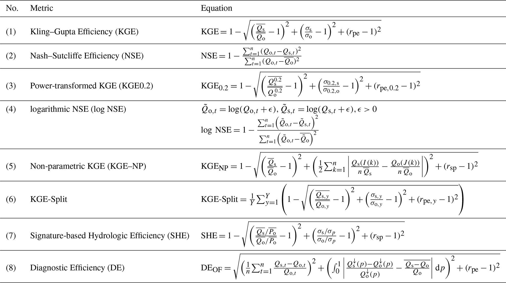
The first two metrics are likely the most common objective functions used in hydrology (Melsen et al., 2025). That is, (1) the Kling-Gupta-Efficiency (KGE; Gupta et al., 2009) and (2) the Nash-Sutcliffe-Efficiency (NSE; Nash and Sutcliffe, 1970) as defined in Table 2. Additionally, we use transformations of the first two metrics that aim to improve the representation of low flows. For KGE, we selected (3) a power transformation because of the known issues with logarithmic transformations (Thirel et al., 2024; Santos et al., 2018). For NSE we selected (4) the logarithmic version because of its long-standing use (Krause et al., 2005); here ϵ is a small positive offset added to streamflow to avoid undefined logarithms at zero flow. In addition, we include four recently developed metrics that intend to improve certain aspects of NSE or KGE or diagnose hydrological model behaviour.

First, this is (5) the non-parametric version of the KGE (KGE-NP; Pool et al., 2018). The major difference with the standard KGE is that the variability component is no longer based on the ratio of variances, but instead replaced by a flow-duration curve-based term. Additionally, the correlation term uses the Spearman rank correlation instead of the Pearson correlation. Pool et al. (2018) argue that the resulting benefit of their proposed metric is an overall better agreement between observations and simulations, except for high flows. Their reasoning is that more information is contained within the metric because the FDC is more complex than the standard deviation and the Spearman rank correlation leads to improvements for low flows. In the equation of (5) I(k) and J(k) indicate time steps in which the kth largest flow occurs in the simulated and observed time series respectively.

Second, another adaption of the KGE, (6) the KGE-Split (Fowler et al., 2018) is evaluated. It is calculated like the regular KGE, but instead of calculating one value for the entire time series, a value for each year is calculated, and the mean over these values becomes the actual objective function value. Fowler et al. (2018) developed it to put more emphasis on dry years, since the typically used “least squares” methods give more attention to high flows rather than low flows. The variables are identical to those used in the KGE, with y indicating the evaluated year and Y the total number of years as shown in Eq. (6).

Third, the (7) signature-based hydrologic efficiency (SHE; Kiraz et al., 2023) normalizes both the bias and the variance term by the mean and variance of the precipitation. Like the KGE-NP, it also uses the Spearman description for the correlation term to improve on the low flow representations. The SHE as used in Kiraz et al. (2023) is defined in Eq. (7).

Fourth, we analyse (8) the Diagnostic Efficiency (DE; Schwemmle et al., 2021) where the bias term is replaced with a mean relative error and the variance term is the integral over all residuals of the relative error based on the flow duration curve. As the name suggests, this metric is designed as a diagnostic tool but will be applied here as an objective function. The general structure, with three parts for bias, variance, and timing, is similar to the KGE, but particularly the variance term proposes an interesting alternative to the KGE. To convert it into a similar objective function as the other candidates we use: DE${}_{\mathrm{OF}}=\mathrm{1}-$ DE, the only metric for which we mark this calibration/analysis distinction in the notation since its two forms differ in formulation rather than in role alone. In Eq. (8), p denotes the exceedance probability and Q^↓(p) the streamflow sorted along the flow-duration curve.

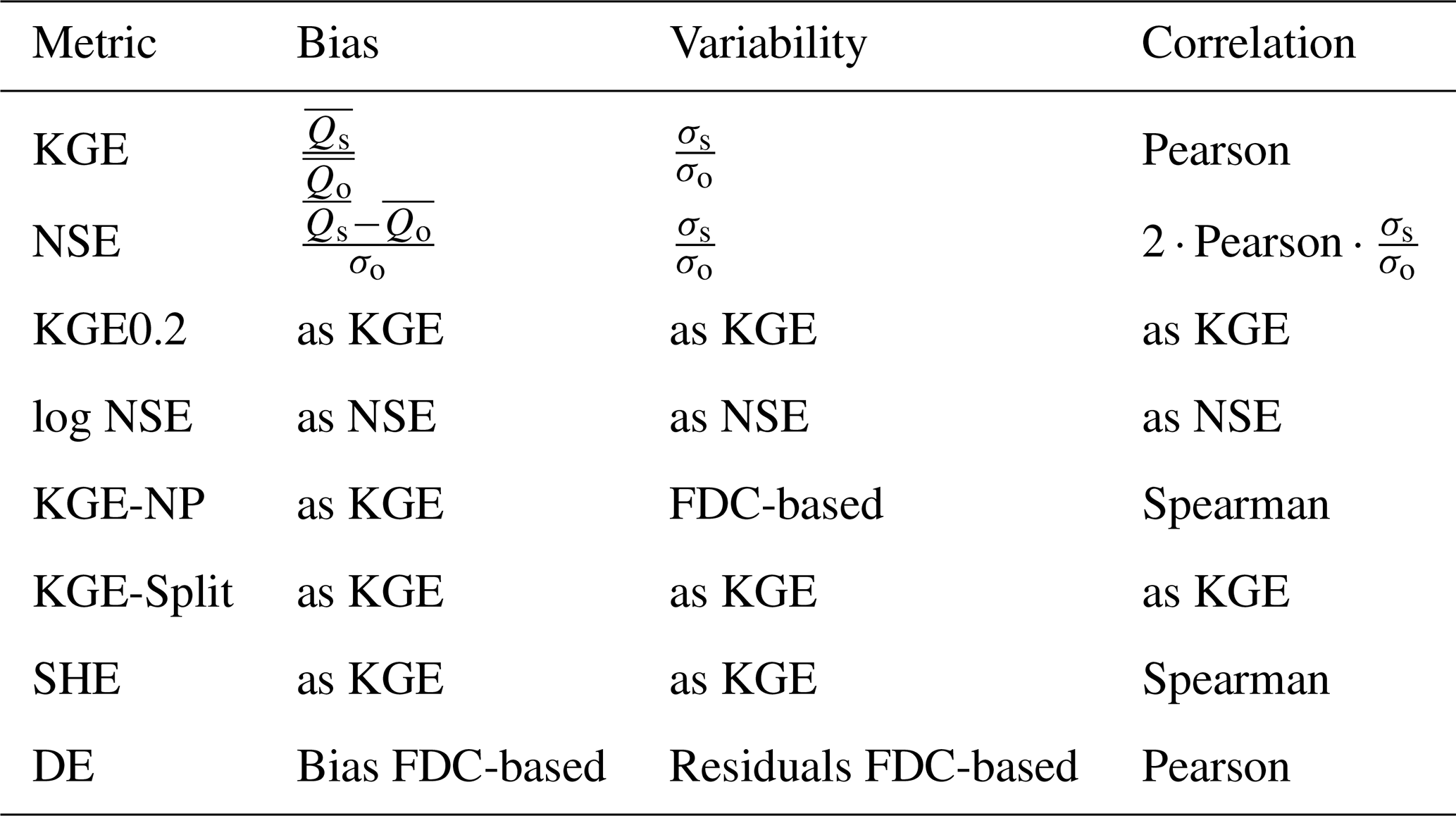
All of the eight used metrics can be disaggregated into three components representing bias, variability and correlation. For an easier overview of the differences between the individual metrics we summarized how they represent each component in Table 3.

Table 3 Overview of the three components of the eight metrics.

2.1.3 Study Catchments

This study uses catchments from the CARAVAN database (Kratzert et al., 2023) which combines several large-sample datasets, include many CAMELS (Catchment Attributes and Meteorology for Large-sample Studies) versions of different countries or regions in a standardized way. While the latest update to CARAVAN now includes more than 20 000 different catchments (Färber et al., 2025) from many existing large-sample hydrology datasets, at the beginning of this study CARAVAN included 2901 catchments. At the time, CARAVAN included catchments in the United States (Addor et al., 2017), Great Britain (Coxon et al., 2020), Brazil (Chagas et al., 2020), Chile (Alvarez-Garreton et al., 2018) and Australia (Fowler et al., 2021) from their respective CAMELS datasets, as well as the LamaH-CE (Central Europe, Klingler et al., 2021) and HYSETS (North America, Arsenault et al., 2020) datasets. CARAVAN provides standardized meteorological forcing, streamflow data, and static catchment attributes (e.g., geophysical, sociological, climatological) with a median data length of 31 years. Our primary goal is to investigate the sensitivity of a large number of different model structures to objective function choice. To keep the analysis manageable (i.e., to “balance depth with breadth” (Gupta et al., 2014), we defined a subset of ten hydro-climatically differing catchments for our analysis. To determine these catchments, we used the climate classification procedure outlined in Knoben et al. (2018) to quantify the aridity, seasonality and fraction snow in each of the CARAVAN basins. We then used a k-means clustering algorithm to divide the catchments into 10 clusters, and selected the catchment closest to each cluster centroid for use in this work. The location of the selected catchments is shown in Fig. 2a and a brief description of some catchment properties is given in Table 4. We also applied a threshold for maximum catchment area of 1000 km² to ensure a more direct influence between discharge, signatures and metrics, because for signatures like the Flashiness Index there might be a dampening effect in larger catchments. The full clustering procedure is described in more detail in Sect. S2.2.

Table 4 Overview of catchment properties for the selected 10 CARAVAN basins. Details in Sect. S2.2.

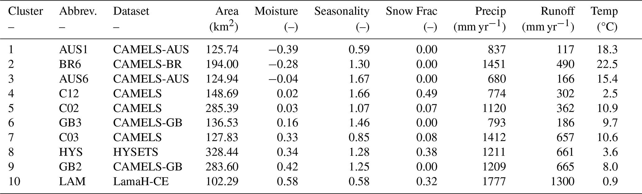
The 10 selected catchments span a wide range of climatic and hydrological settings. They differ substantially in aridity and mean temperature, ranging from humid, cool basins such as LAM and HYS (moisture index ≈0.3–0.6, mean temperatures near 0–4 °C) to warm catchments like AUS1 and BR6 (negative moisture indices indicating high aridity, mean temperature > 18 °C). Snow fraction varies substantially, from snow‐free catchments in Australia and Brazil to snow‐influenced basins such as C12 and LAM. Precipitation and runoff also contrast strongly, with wetter, high‐runoff regions (e.g. LAM, GB2) versus more arid, low‐runoff sites (AUS1, BR6), illustrating the climatic and geographic diversity captured by the dataset and clustering approach. To avoid known issues with the ERA5-based potential evapotranspiration (PET) estimation from CARAVAN (Clerc-Schwarzenbach et al., 2024), we are using the provided alternative based on Penman-Monteith. We have compared the CARAVAN data for precipitation, potential evapotranspiration and temperature against the native forcing data provided by each catchment's source dataset (e.g. CAMELS, CAMELS-AUS, CAMELS-BR, CAMELS-GB, HYSETS, or LamaH-CE) and found no systematic bias, confirming the CARAVAN forcing was of sufficient quality for consistent use across all catchments (details in Figs. S3–S12 in the Supplement).

2.2 Model Calibration Procedure

All models were run on daily time step and calibrated with the Covariance Matrix Adaptation Evolution Strategy (CMA-ES) algorithm by Hansen et al. (2003) as implemented in the MARRMoT Toolbox. We used a 10-year time period from 2004 to 2014 for calibration and a 10-year time period from 1993 to 2003 for evaluation with a one-year warm-up period each. The evaluation period of the catchment AUS6 had to be shortened to eight years (1981–1988) because of data gaps; the calibration period covers 1990–1999. We conducted 18 800 ($\mathrm{5}\times \mathrm{47}\times \mathrm{8}\times \mathrm{10}$) calibration runs to calibrate each of the 47 models on all eight metrics in each of the ten catchments. To consider parameter uncertainty we calibrated each combination on five different seeds and retained the best 500 parameter sets across all seeds.

For all analysis, we focus on the calibration period only, because it provides the closest connection between objective function choice and resulting model behaviour. If objective functions cannot produce accurate signatures during calibration, it is unlikely that they will systematically do so during evaluation. We provide additional plots showing model and signature performance during the evaluation period in the Supplement (Figs. S13/S14).

2.3 Model Benchmarking

We establish a baseline performance benchmark to remove poorly performing models from further analysis. Based on earlier arguments and examples (Seibert, 2001; Schaefli and Gupta, 2007; Knoben et al., 2020; Knoben, 2024), we use an ensemble of benchmark models that can be used to establish the minimum performance a model should exceed. The HydroBM package (Knoben, 2024), provides 22 benchmark models that can easily be used. They cover three broad categories: benchmarks derived from streamflow data, such as the daily mean flow timeseries, which accounts for seasonality; benchmarks derived from rainfall-runoff ratios; and very simple empirical models that approximate aggregated catchment behaviour. For each catchment, we compute the performance of the timeseries these benchmark models create by comparing it to the observed discharge data in the calibration period. By calculating all eight performance metrics we can identify which benchmark model yields the highest performance for each metric and catchment. This performance will be used as the benchmark to beat. Model runs that fail to outperform this highest benchmark are excluded from further analysis, ensuring that only sufficiently reliable models are carried forward to the analysis of signature performance. For catchments with a snow fraction larger than 30 % we additionally remove all models without a snow module from the analysis should they manage to beat the benchmark.

2.4 Signature Selection

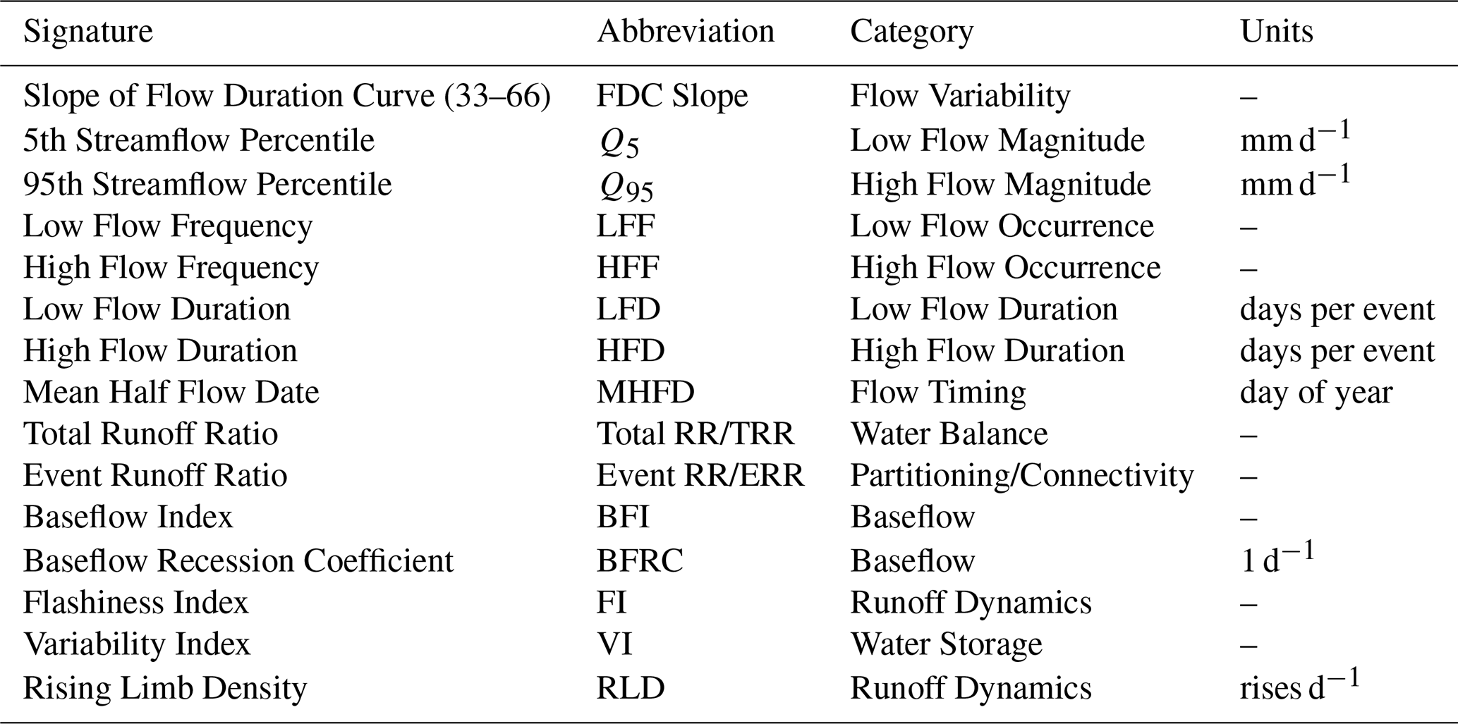
We selected 15 streamflow signatures to investigate the extent to which objective function choice influences a model's ability to replicate streamflow signatures. Our goal with this selection is to cover different aspects of the flow regime, as well as a range of hydrological processes (McMillan, 2020). The selected signatures are shown in Table 5 and were all calculated using the TOSSH toolbox (Gnann et al., 2021), a more detailed description of each signature can be found in Sect. S2.5. Most of the considered signatures describe streamflow properties such as the slope of the flow duration curve (FDC Slope, 33rd–66th exceedance percentiles), the 5th and 95th streamflow percentiles (Q₅ and Q₉₅), the high and low flow duration (HFD & LFD) and frequency (HFF & LFF) as well as the mean half flow date (MHFD). The slope of the FDC describes the variability of the streamflow regime, indicating how quickly a river responds to rainfall events and how sustained the flows are during dry periods. Representing it correctly therefore indicates a good representation of in-catchment storage and flashiness behaviour. The 5th and 95th streamflow percentile describe the magnitude of low and high flows. Representing these signatures well indicates a good representation of extreme flow behaviour, while representing the high and low flow duration and frequency well ensures that also these important characteristics of extreme flow can be met. The MHFD helps to determine if the general timing and seasonality of streamflow is represented well. Additionally, we evaluate the impact of the objective function on the total runoff ratio (Total RR), event runoff ratio (Event RR), baseflow index (BFI), baseflow recession coefficient (BFRC), flashiness index (FI), variability index (VI) and rising limb density (RLD). These are intended to deliver information on the different catchment processes such as the general water balance (Total RR), individual storm responses (Event RR), the baseflow processes (BFI, BFRC) or general water storage behaviour and runoff dynamics (flashiness index, variability index, rising limb density).

Table 5 Overview of selected signatures.

2.5 Analysis of Objective Function Influence

2.5.1 Signature Error Metric

As most signature values have individual ranges and can differ substantially between catchments, we analyse normalized signature errors for better comparison. We first define the error at the level of individual retained runs, then aggregate it (additional details are provided in Sect. S2.6).

For a single retained run (one catchment, one model, one objective function, one parameter set), the signature error is the deviation of the simulated signature from the observation,

$$\begin{array}{}\text{(9)}& e_{ijkr}=S_{ijkr}-y_j,\end{array}$$

where S_ijkr is the simulated signature value for model i, catchment j, objective function k, and retained run r, and y_j is the observed signature value for catchment j.

To place signatures of different magnitudes on a comparable axis, errors are normalized on a per-catchment basis. The normalization denominator D_j is the largest absolute typical error across objective functions for that catchment,

$$\begin{array}{}\text{(10)}& D_j=\underset{k}{max}\left(\left|{\stackrel{\mathrm{‾}}{e}}_{jk}\right|\right),\end{array}$$

where ${\stackrel{\mathrm{‾}}{e}}_{jk}$ is the typical (median) error of the retained ensemble, obtained by first taking the median over the retained runs of each model and then the median across models,

$$\begin{array}{}\text{(11)}& {\stackrel{\mathrm{‾}}{e}}_{jk}=\begin{array}{c}\mathrm{med}\\ i\end{array}\left(\begin{array}{c}\mathrm{med}\\ r\end{array}\left(e_{ijkr}\right)\right).\end{array}$$

The sequential median ensures that each model contributes equally to the typical error, independent of how many of its retained runs pass the benchmark.

The run-level normalized error is then

$$\begin{array}{}\text{(12)}& e{m}_{ijkr}={\displaystyle \frac{e_{ijkr}}{D_j}}={\displaystyle \frac{S_{ijkr}-y_j}{\begin{array}{c}max\\ {}_k\end{array}\left(\left|\begin{array}{c}\mathrm{med}\\ {}_i\end{array}\left(\begin{array}{c}\mathrm{med}\\ {}_r\end{array}\left(S_{ijkr}-y_j\right)\right)\right|\right)}}.\end{array}$$

Positive values indicate overestimation and negative values underestimation of the observed signature. The normalization is performed catchment by catchment, so that an objective function that is the most biased in all catchments would reach ±1 at the median level. Because D_j is set by the typical (median) error while individual runs may deviate further, run-level values can exceed $[-\mathrm{1},\mathrm{1}]$.

Aggregating over the retained ensemble gives a catchment- and objective-specific error metric. Since D_j is independent of model and run, the median passes through the normalization,

$$\begin{array}{}\text{(13)}& {\mathrm{EM}}_{jk}=\begin{array}{c}\mathrm{med}\\ i\end{array}\left(\begin{array}{c}\mathrm{med}\\ r\end{array}\left({\mathrm{em}}_{ijkr}\right)\right)={\displaystyle \frac{{\stackrel{\mathrm{‾}}{e}}_{jk}}{D_j}},\end{array}$$

which by construction lies in $[-\mathrm{1},\mathrm{1}]$, with 0 indicating that the observed value is matched exactly.

Finally, aggregating across catchments yields a single value per signature and objective function, which is used to identify the objective function that best represents each signature,

$$\begin{array}{}\text{(14)}& {\mathrm{EM}}_{k,\mathrm{abs}}=\begin{array}{c}\mathrm{med}\\ j\end{array}\left(\left|{\mathrm{EM}}_{jk}\right|\right).\end{array}$$

2.5.2 Statistical Testing of Objective Function Influence

To better understand which signatures are most affected by the objective function choice, we conducted a paired sample t-test: a pairwise comparison for two objective functions at a time by testing their median value of signature values across catchments. The null hypothesis for the t-test used here is H₀: The mean values of the distributions are equal to each other. With 8 objective functions this leads to $\left(\begin{array}{c}\mathrm{8}\\ \mathrm{2}\end{array}\right)=\frac{\mathrm{8}\cdot \mathrm{7}}{\mathrm{2}}=\mathrm{28}$ pairwise comparisons for each signature. The signature value entering each comparison is the per catchment median error EM_jk (Eq. 13), in which model and parameter-set variability have already been collapsed through the sequential median (Sect. 2.5.1); the test thus pairs the two objective functions catchment by catchment across the ten catchments, and the retained top-500 runs are not treated as independent samples.

This analysis highlights which signatures are most strongly influenced by the choice of objective function. We report the resulting p-values for each pairwise comparison and consider differences statistically significant at α=0.05. Not all distributions are expected to differ significantly, as some objective functions are likely to produce similar results. Based on these outcomes, we restrict subsequent analyses to signatures that are commonly significantly impacted by the choice of objective function, which we define as 40 % of the p-values being lower than 0.05.

2.5.3 Random Forest for Attribute Importance

We apply random forest (RF) regression to assess the relative importance of catchment, objective function (OF), and model choice. We consider two complementary configurations. In the first, the response is the median simulated signature value across the retained ensemble per (model, catchment, OF) combination; in the second, the response is the corresponding median signature error against the observation (taken from Sect. 2.5.1). In both cases the predictors are the categorical factor indices for model (i), OF (k), and catchment (j).

We used the TreeBagger implementation in MATLAB with 500 trees and regression mode, extracting out-of-bag permuted predictor importance scores. Negative importance values, which indicate no predictive contribution, were set to zero. For each signature and configuration, importance values were normalized to sum to one, providing a direct measure of the relative influence of the three factors.

3 Results

The following sections will cover the outcomes of the benchmarking procedure (Sect. 3.1). Based on this, the general distribution of signature representation (Sect. 3.2) for (i) the detailed example of Total Runoff Ratio and (ii) all signatures (aggregated over the models) are shown. Afterwards, we will use the error metric (Eq. 13 from Sect. 2.5.1) to highlight the skills and shortcomings of each objective function in Sect. 3.3. Further analysis is then used to test the statistical significance of objective function influence (Sect. 3.4) and assess the relative predictive importance of objective function choice (Sect. 3.5). Lastly, we use the aggregated error metric (Eq. 14 from Sect. 2.5.1) to find the best performing objective functions regarding signature representation.

3.1 Benchmarking the Models

Figure 3 shows the performance of all 47 calibrated models with their 500 best parameter sets (violins) compared to the highest calculated benchmark (red dash) as described in Sect. 2.3.

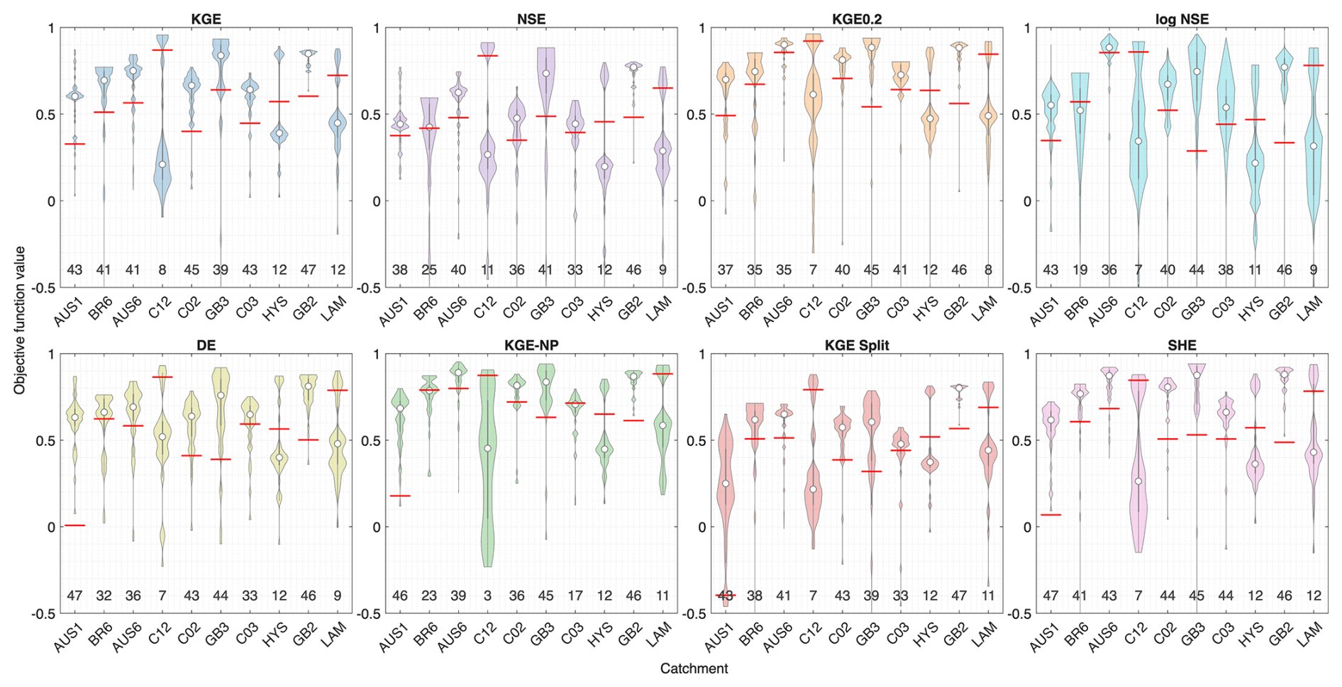
Figure 3 Benchmark Performance (driest catchment on left to wettest catchment on right). The distribution shows the objective function values across the top 500 parameter sets (across all calibrated seeds) for all 47 models and the red line shows the highest benchmark score of the objective function. The numbers below each violin indicate the number of models that outperform the benchmark with at least one of their parameter sets. The white circles indicate the median of the data in the violin.

The number of models that beat the benchmark varies considerably across catchments and objective functions (number shown below each violin). In three catchments (C12, HYS, LAM) the number of models is comparatively low. The explanation is a strong snow influence, which produces seasonality that only the 12 of the 47 MARRMoT models that include a snow module can accurately reproduce. In other catchments, most models beat the benchmark, and the models that fail may be missing important process controls (e.g., groundwater representation) though this is more difficult to diagnose than the snow cases. In a handful of cases all models can beat the benchmark (e.g. GB2 for the KGE objective function), and for every combination of catchment and OF, there are at least 3 models exceeding the benchmark ensemble. As may be expected, more complex models (more parameters and stores), tend to outperform the benchmark more often and were retained more frequently (result not shown).

3.2 How accurate are the signature representations when different objective functions are used?

To begin the analysis of how objective functions affect hydrological adequacy, we compare the simulated signature values with the observed signature values for all eight objective functions. Figure 4 shows the distribution of absolute errors (y-axis) over all catchments (x-axis) for each metric (subplots) for one of the 15 signatures, the Total Runoff Ratio. The plots for all other signatures can be found in Sect. S2.9 (Figs. S16 through S29).

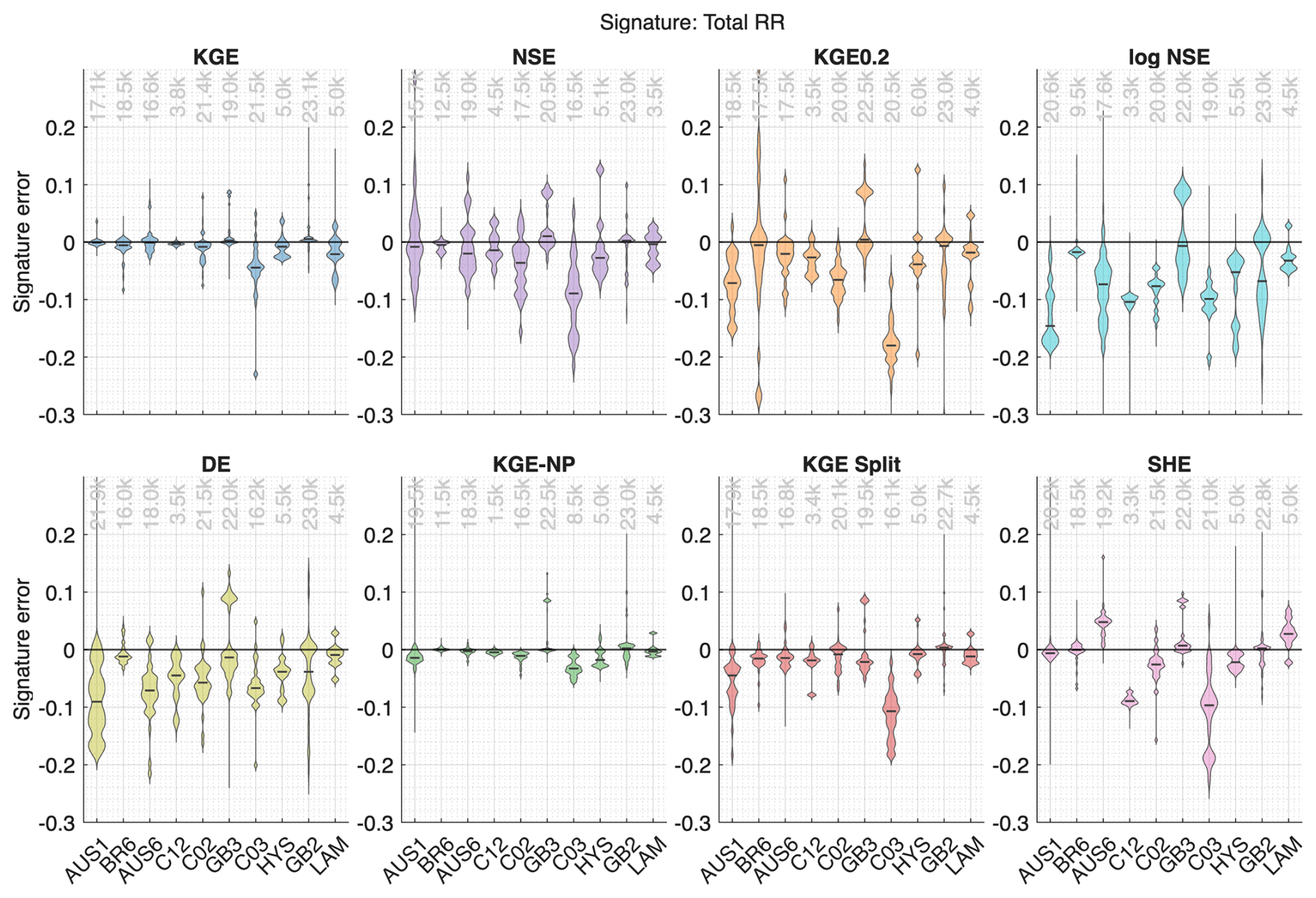
Figure 4 Signature error (simulated – observed) on Total RR values for all objective functions. The shown distributions include all models and their 500 best parameter sets that passed the benchmark. The numbers above the violins indicate the number of runs (model × parameter set) shown within each violin. A number of 23 500 would indicate all models and parameter sets were retained.

In Fig. 4, there are three things of note. First, the location of the violin plots shows whether the signature values are underestimated (negative values), overestimated (positive values) or relatively unbiased (centered around zero). Second, the size of the violins indicates whether the signature predictions are well-constrained (short violin) or not (long violin). Third, the catchments are ordered from driest (left) to wettest (right) indicating if signature error correlates with climate.

There is no clear pattern in Runoff Ratio errors related to the catchments' aridity values. Instead, there appear to be two categories of results: objective functions that return mostly unbiased models in all catchments (KGE and KGE-NP), and objective functions where the signature representation of the resulting models varies strongly per catchment (e.g. NSE: relatively unbiased in some basins, large variability in signature errors in others). The KGE-NP constrains the variability within the models much better and is therefore assessed as the best available objective function for the general water balance as represented through the Total RR signature. For the remaining six objective functions, the Runoff Ratio tends to be underestimated and positive errors are relatively rare. This means that generally the models tend to put too much water into storage and/or evaporation or other sink terms, which may become relevant when modelling climate change impacts.

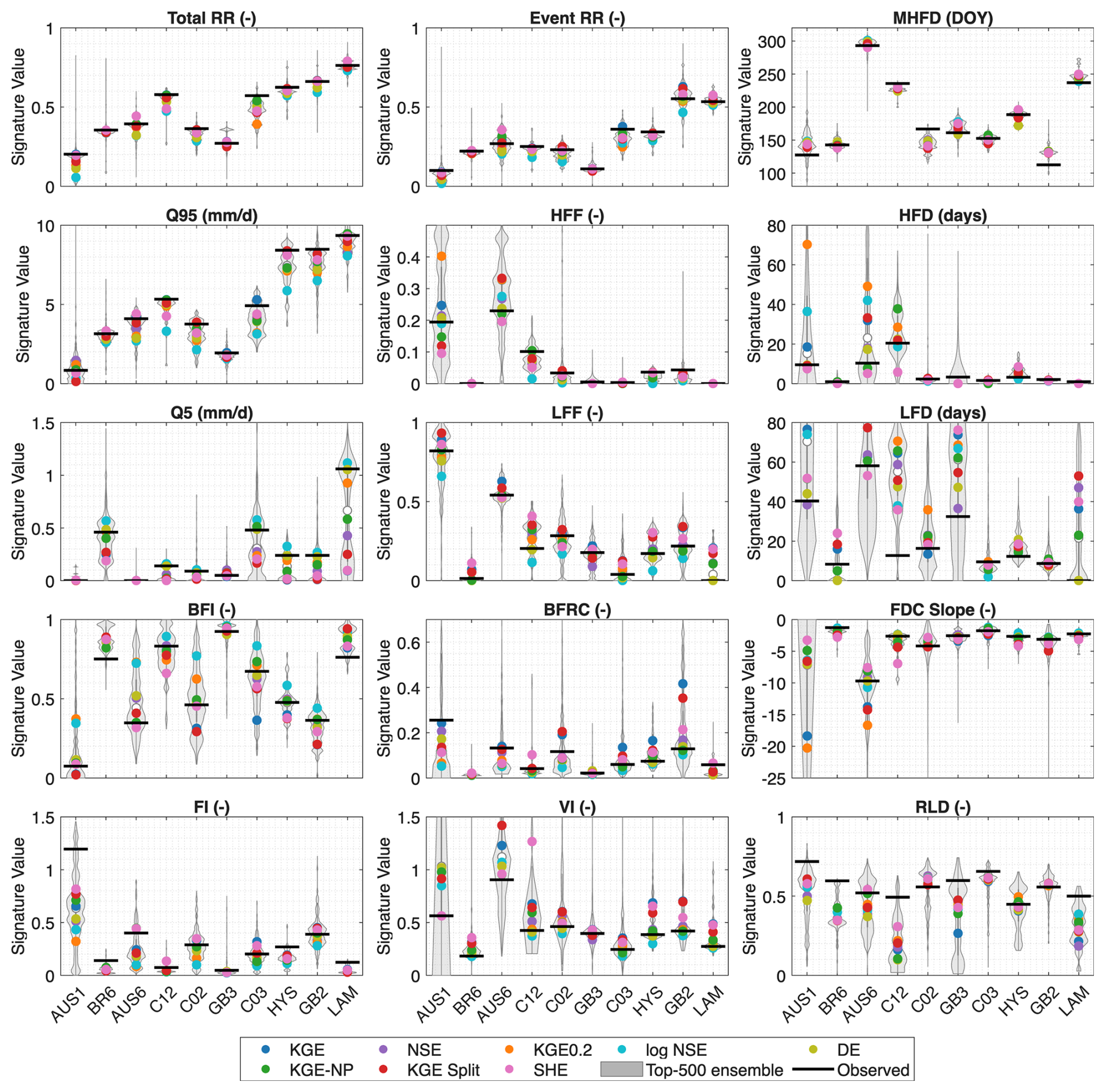
Figure 5 Comparison of signature representation capabilities across the different objective functions. The coloured points represent the median signature (across all retained models calibrated with a specific OF). The black dashes indicate the observed signature values. The grey violins represent the variability of the modelled signature values across the retained models with their top 500 parameter sets. In catchment AUS1, the observed value for the FDC slope is NaN, because the observed flow is 0 mm d⁻¹ for more than 66 % of the time steps in calibration period.

To show the results for more signatures in an aggregated way, Fig. 5 shows the median simulated signature value over all models above the benchmark (underlying data can be seen in Figs. S16–S29). The median was chosen to achieve the most representable summary of the model ensemble, which is not susceptible to outliers. This gives an overall impression on the capability of the different models to represent the hydrological signatures of interest. It also allows a first impression of the impact different objective functions have on signature representation. In Fig. 5, the coloured dots indicate the median modelled signature value for each objective function, while the black line shows the signature values calculated from observations. The grey violins indicate the variability in the modelled signature value if all individual model results with their 500 best parameter sets are considered (every model that beats the benchmark for any objective function). The plot therefore allows insights on how well a signature value can generally be represented through the different tested models and gives a first impression on the influence the objective function has on these representations. The x-axis denotes the 10 selected catchments and the y-axis gives the signature value in its native unit (see Table 5).

Initially, we can use this plot to compare the violin ranges to the observed values of signatures. For the vast majority of cases, the observed value is always within the boundaries of the model ensemble, which indicates that the tested conceptual models are able to capture the hydrologic variability across diverse catchments. The spread of the coloured dots around the observed values indicates different degrees of accuracy in the signature representation depending on the calibration metric used. For some signatures, the range of signature values is notably smaller (e.g. Total RR) than for others (e.g. Rising Limb Density). There are signatures (e.g. Q₉₅, BFI) where the objective functions differ strongly from each other and signatures where different objective functions lead to similar modelled values (e.g. MHFD, HFD). To move beyond these very broad conclusions, the next section will use the previously introduced error metric (Eq. 13 from Sect. 2.5.1) to assess the relative skill of each objective function in more detail.

3.3 Which objective functions show strengths or weaknesses for a specific hydrological signature?

In this section we use Eq. (13) to normalize the signature errors using the observed signature value. Figure 6 shows the normalized error in signature representation for all objective functions. Generally, we can see that the performance varies largely depending both on the signature (each violin in a plot) and catchments/models (within the violins).

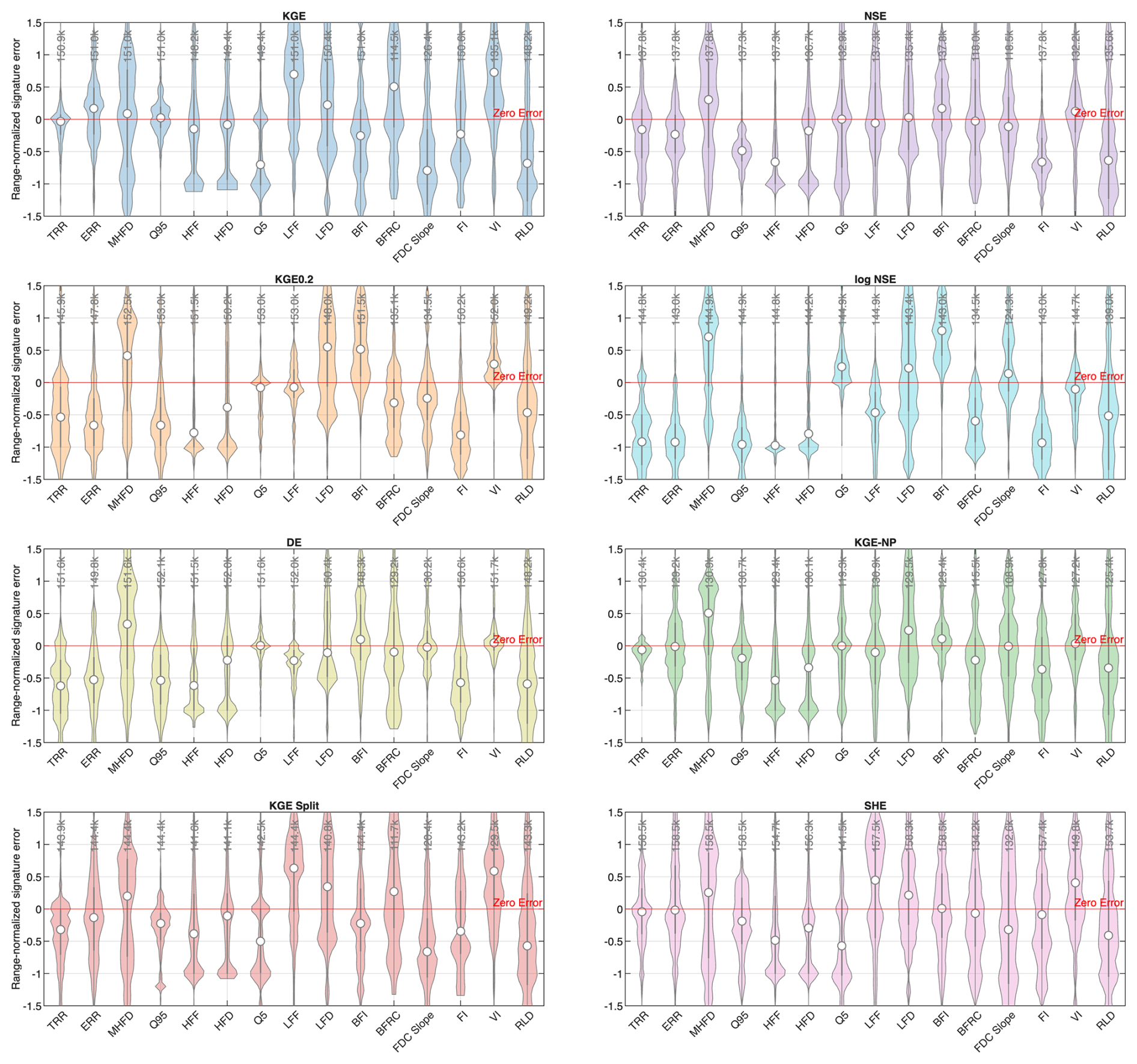
Figure 6 Error Metric as given in Eq. (13) for all Objective Functions. The error metric is calculated for each objective function (subplot) per signature (x-axis) and catchment (data in violin). A value of 0 indicates no error in signature representation. A value of −1 or +1 would indicate a performance equal to the most extreme over/underestimation for the median across models and runs. As we are showing the top 500 runs for all benchmark-exceeding models explicitly, the values can exceed these boundaries. A number of 235 000 would indicate all models and parameter sets were retained.

The KGE in Fig. 6 has good performance for the Total Runoff Ratio and the high flow percentile Q₉₅ (violin has a smaller spread around the zero error line). This does not only apply to the median performance (white dot in the violin) but also has a high consistency among catchments and parameter sets (violin spread). However, particularly for the low flow percentile Q₅, LFF, FDC slope, and Variability Index the representation obtained from calibrating to KGE relative to the other objective functions is often worse.

The NSE performs mediocre on almost all of the evaluated signatures: the range within catchments and runs (spread of each violin) is often large. This indicates that the suitability of the NSE metric can be very catchment- and model-dependent. HFF, FI, RLD and Q₉₅ are usually underestimated by models calibrated on the NSE. Compared to the KGE, the performance on Q₅, and FDC slope is typically better.

For KGE0.2 and log NSE, we see similar patterns in signature error. Both (KGE0.2 and log NSE) underestimate the runoff generation and high flows as well as the reactivity of the catchment (Flashiness Index). The log NSE is often the worst objective function among the eight investigated, indicated by high or low values. Both metrics show improvements compared to the KGE for FDC Slope and Q₅, but not necessarily for low flow duration (LFD) and frequency (LFF). It is important to notice that the FDC Slope can also be met well if the runoff is systematically biased, which is the case with underestimation here. In many of the evaluated 15 signatures, the KGE0.2 shows a better performance than the log NSE (violin closer to 0).

The diagnostic efficiency generally performs similarly to the KGE0.2. It mainly improves representation of the BFI but has comparable issues for Total RR and Q₉₅. Compared to the KGE, the errors are constrained better across catchments (smaller violins). In conclusion, the diagnostic efficiency proves to be a viable alternative for low-flow calibration, while offering benefits on additional signatures (such as BFI and VI).

The non-parametric version of the KGE performs worse than the KGE on high flows, but improves other signatures strongly, such as the BFI, FDC Slope, Q₅ and LFF. The KGE-NP is among the objective functions that perform best overall. The expectations (general improvement due to more information being included) for KGE-NP are thus largely met, with the main benefit being better incorporation of flow variability for a larger fraction of flow percentiles.

KGE-Split performs similar to the regular KGE, though shows a tendency towards larger errors. Like the NSE, it has no signature that is represented both more accurately and consistently than alternative objective functions. Compared to the regular KGE, there are slight improvements on selected signatures (FDC Slope, BFI, Variability Index).

Lastly, the SHE is one of the objective functions with the largest range in signature representation. The general patterns are similar to the KGE (as expected due to their similar formulation), except for selected signatures like FDC Slope. This indicates that a change from value-based correlation to rank-based can be influential for signature representation.

The violin plots also show that some signatures are affected very little by the choice of objective function such as the Rising Limb Density and the Mean Half Flow Date, which is indicated by a similar distribution among objective functions. This suggests that either the models or the catchment mainly influence the results. As the signature value cannot be simulated well from any of the models, this shows the limits of objective function influence.

The Supplement (Figs. S30 and S31) includes plots on the analysis with 25 and 100 parameter sets in comparison to the 500 used here. Since the results remain comparable, we assume that parameter uncertainty plays only a minor role here. Additionally, the SM also provides an example of the error metric collapsed to one value per catchment as it is being used in the assessment of overall skill (Fig. S32), which emphasizes the differences more, but does not account for model- and run-level uncertainty.

3.4 Does the objective function choice significantly affect signature representation?

This previous section showed the skills and shortcomings of the individual objective functions regarding signature representation. However, it is not easy to assess whether the observed influences that were described can be considered significant for the process representation. To investigate this, we apply statistical testing in this section. Figure 7 shows the distributions of p-values when testing the significance of signature values calculated with different OFs against each other.

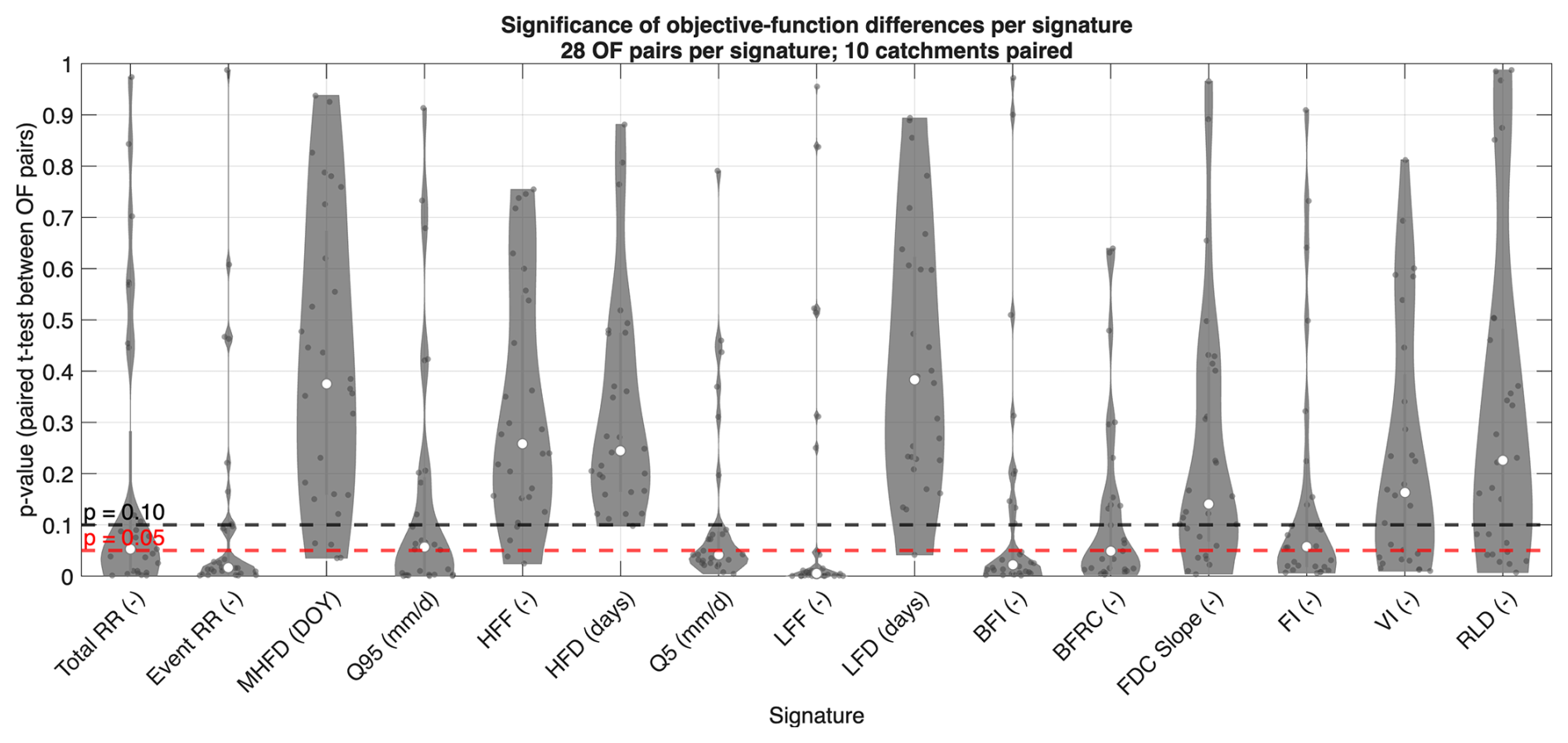
Figure 7 Significance Test between signature representations of the different objective functions. The red (p=0.05) and black (p=0.1) lines indicate commonly used significance thresholds. Every signature that is below these values can be considered to have a statistically significant difference between the paired samples of signature value distributions (in other words, the two objective functions in the pair lead to statistically different values for the signature across all included models).

All signatures show a large range in p-values, which implies that there are both objective functions which have similar and different representation for each signature. Some OFs typically behave similar, e.g. the distributions of KGE0.2 and log NSE are often comparable for low flow signatures. Figure 7 shows that the choice of objective function strongly affects the following signatures: the Total RR, Event RR, Q₅, Q₉₅, LFF, BFI, BFRC, and the Flashiness Index. For the remaining 7 signatures (Low and High Flow Duration, HFF, Mean Half Flow Date, FDC Slope, Variability Index, Rising Limb Density) a change of objective function does not lead to a clear shift in signature representation for most of the combinations of objective functions. Table S3, Sect. S2.11 shows the frequency of objective function pairs reaching p-values of below 0.10 or 0.05 respectively.

By comparing Fig. 7 to Fig. 5 we can conclude that there can be considerable spread in the representation of the signatures that do not show a significant difference. This is because the spread for signatures like Low Flow Duration, Variability Index, or Rising Limb Density is often not consistent, meaning that when comparing the distribution of signature values of two objective functions with each other, there is variation as to which one has higher or lower values. Therefore, the significance often shows no significant impact because the signal is not clear. The significance test indicates that the variation is not driven by the objective function and we speculate that in these cases other influences such as catchment characteristics or models drive the spread seen in the signature representation.

3.5 What controls simulated signature values?

Figure 8 shows the random forest feature importance for catchment, model, and OF (parameter-set variability is considered as a median value across the 500 parameter ensemble).

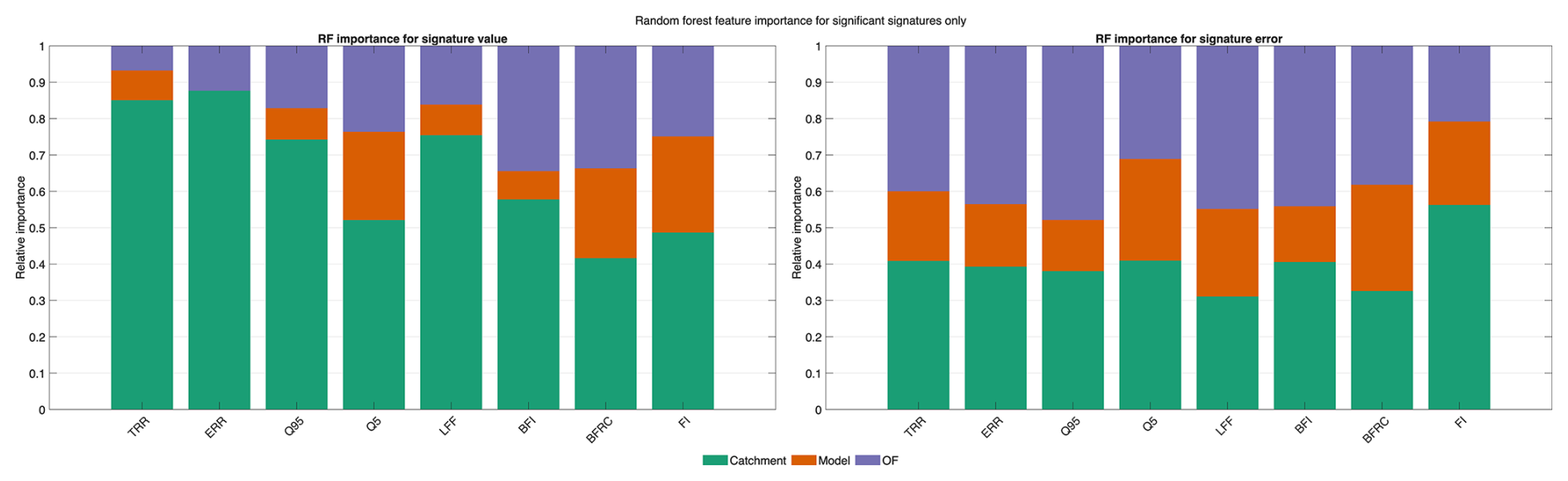
Figure 8 Random Forest Feature Importance based on predicting the simulated signature value (left) and signature error (right) using the median over the top 500 performing runs.

Reading the value and error panels together clarifies the role of each factor. Catchment dominates the absolute signature values which is expected, since the basins were deliberately chosen to be hydroclimatically diverse. However, its importance for the signature error is markedly lower and roughly equal across the eight signatures. Objective function has comparatively limited control over the value, yet its importance rises for the error, most strongly for Total RR, Event RR and Q₉₅, and typically exceeds that of model choice. Model structure contributes throughout and gains relevance for low-flow and baseflow signatures (BFI, BFRC, Q₅), where together with OF choice it challenges the catchment as the leading predictor. The pattern is consistent across signatures: the catchment largely controls the order of magnitude of the simulated signatures, but the choice of objective function and model structure play a large role in how closely those magnitudes match the observations.

3.6 Overall Skill of Signature Representation

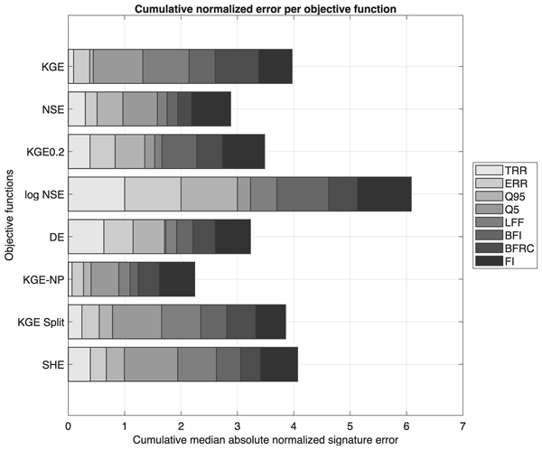
Our results suggest that all objective functions can represent some signatures well while having shortcomings in others. This implies that, when selecting an objective function, there is not a single choice that will ensure realistic values across the spectrum of streamflow signatures we investigated. Yet, we can identify objective functions that generally have good process representation across several signatures by investigating the accumulated errors of all significantly influenced signatures as shown in Fig. 7. For this, we use Eq. (14) to get one median error value per signature and objective function. Figure 9 shows this accumulated error for the eight tested objective functions.

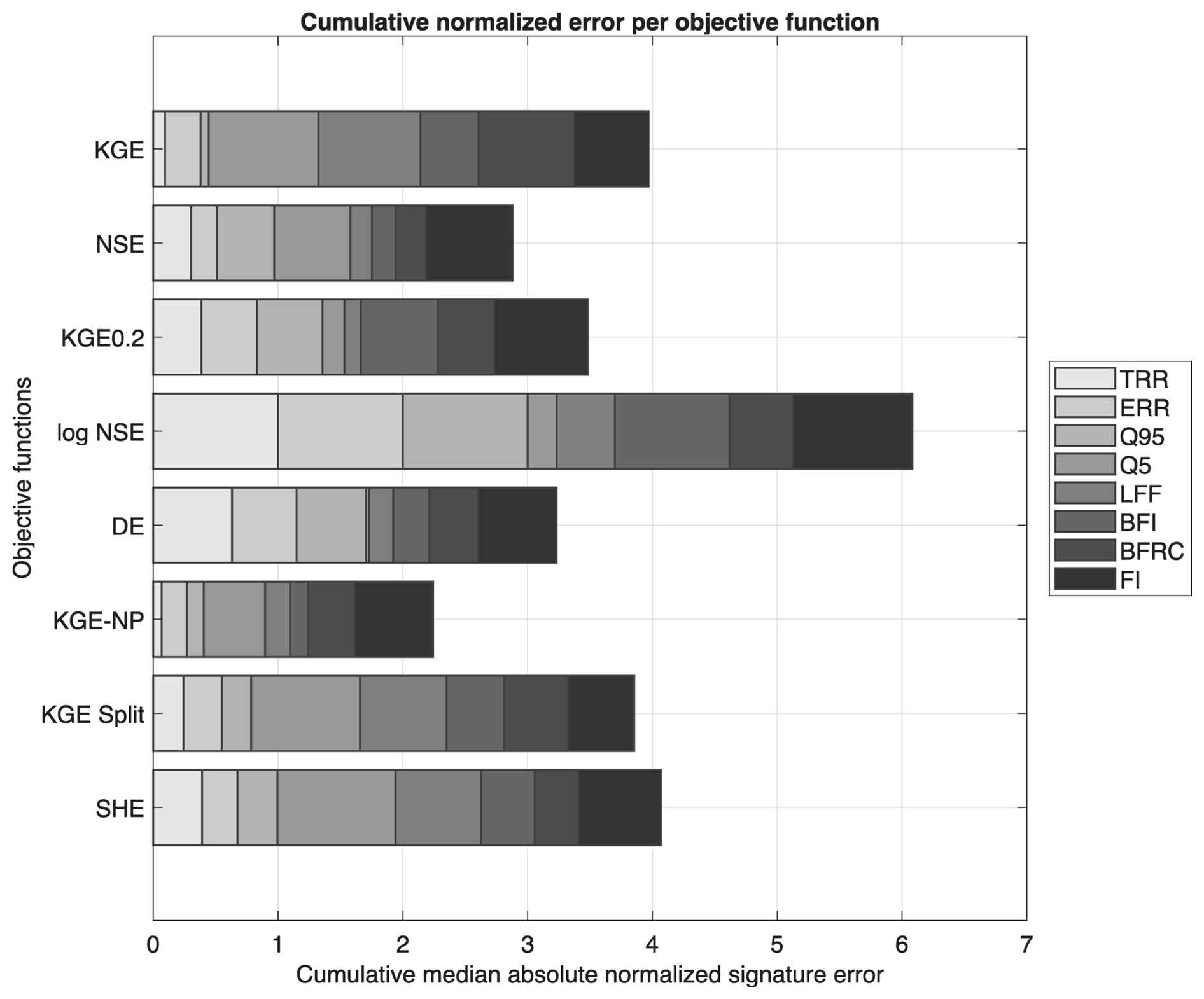
Figure 9 Cumulative error in significantly influenced signatures per tested objective function. This was calculated using the median across the top 500 parameter sets per model.

The modeled overall error in signature representation varies strongly depending on the objective function chosen. Considering the entire set of signatures with significant metric influence, the KGE-NP, NSE, and DE show the best overall performance. Conversely, this study identifies the log NSE as having the overall largest errors. This, however, does not immediately imply that certain OFs should not be used as each has its strengths and weaknesses. As shown before, the KGE is the best metric for high flow conditions (small errors for Q₉₅) and works well for Total RR, while it has considerable weaknesses for low flow representation (e.g. BFI, BFRC and Q₅). And while the log NSE performs decently on low flow conditions (Q₅) it is considerably worse for most other significant signatures. Similarly, despite the KGE-NP showing the best overall performance, it still comes with weaknesses in Q₅ and FI representation.

As a robustness check, we repeated the central signature-error and objective-function ranking analysis for the evaluation period. The evaluation-period results broadly confirm the calibration-period patterns. As expected, signature errors generally increase during evaluation, but the relative strengths and weaknesses of the objective functions remain largely similar. In particular, the ranking of objective functions for the OF-sensitive signatures is comparable between calibration and evaluation, suggesting that the main conclusions are not an artefact of calibration-period performance alone. Detailed evaluation period results are provided in the Supplement (Fig. S33).

4 Discussion

We structured our discussion into three parts. First, we synthesize the main takeaways for signature representation across models, catchments, and objective functions. We condense our findings into some practical recommendations. Second, we discuss the correlation between different signatures and how they relate to the identified impact of objective function choice. Third, we outline the limitations of our study and potential future work.

4.1 Main Takeaways and Practical Recommendations

Across 47 model structures and 10 hydro-climatically diverse basins, OF choice exerts a systematic but selective influence on simulated streamflow signatures. A paired significance test indicated that 8 of 15 signatures vary significantly with OF choice (Fig. 7), whereas timing descriptors such as MHFD and RLD are largely OF-insensitive. This may in part be due to the selection of OFs, as objective functions that specifically target time offset (e.g Mean Absolute Peak Time Error; MAPTE) are less frequently used (Ehret and Zehe, 2011) than the OFs we did select. Generally, no single OF excels at all tested signatures. Considering the cumulative error across OF-sensitive signatures (Fig. 9), KGE-NP yields the lowest overall error, with NSE and DE performing competitively in some basins but less consistently across signatures. The DE and the selected transformed OFs (log NSE, KGE0.2) reproduce low flow metrics better (Q₅, LFF), but particularly the latter come with considerable tradeoffs in the representation of other signatures such as Total RR, baseflow related signatures, or HF signatures.

Our analysis hence contributes to the available information of specific strengths and weaknesses of individual OFs. KGE, for example, most reliably reproduces Q95 (Mizukami et al., 2019), and KGE-NP is one of the best OFs for total runoff ratio and for the baseflow index (BFI), while sharing the best representation of baseflow recession (BFRC) with DE. Log NSE, in comparison, showed few strengths for representing hydrological signatures in our experiments, performing well only on Q₅. However, DE reproduces Q₅ comparably while carrying a smaller overall error, which is why we recommend DE for that signature and DE or KGE0.2 for low-flow frequency rather than the transformed NSE. The KGE-Split, NSE, and SHE show a balanced error field with individual differences in cumulative errors (Fig. 9); within this group, NSE is the most reliable for Event RR, where it ranks alongside KGE-NP, and KGE-Split is otherwise unremarkable but reproduces the Flashiness Index best of all tested OFs.

We also compared the influence of OF choice on signature representation with other influencing factors such as catchment characteristics or model structure choice. Our random-forest analysis showed that catchment characteristics are the dominant control of signature representation, with OF choice typically more influential than model choice (Fig. 8). Model choice does, however, gain relevance for signatures connected to low flow or baseflow representation, while OF choice seemed especially relevant for baseflow related signatures.

When reducing the impact of the conducted catchment selection by training the random forest on signature errors instead of signature values, the importance of the objective functions and model selection increased considerably for most signatures. This indicates the importance of appropriate objective function and model choice across hydro-climatic differences, which may be an overlooked aspect in large sample studies, potentially indicating a path for more detailed evaluation using signatures and their deviations. The broader analysis also contextualizes for which characteristics objective function choice can be influential, while others are predefined by catchment (MHFD) or a combination of catchment and model (RLD), which is shown in Fig. S34. In summary, our results support the argument for a purpose-based model calibration, that considers specific aspects of the flow regime, rather than defaulting to a familiar single metric (Mai, 2023; Jackson et al., 2019).

Table 6 Recommendations for objective functions that can represent the 15 considered signatures well according to our study results. Where a signature was not significantly affected by OF choice, we report “not significant”.

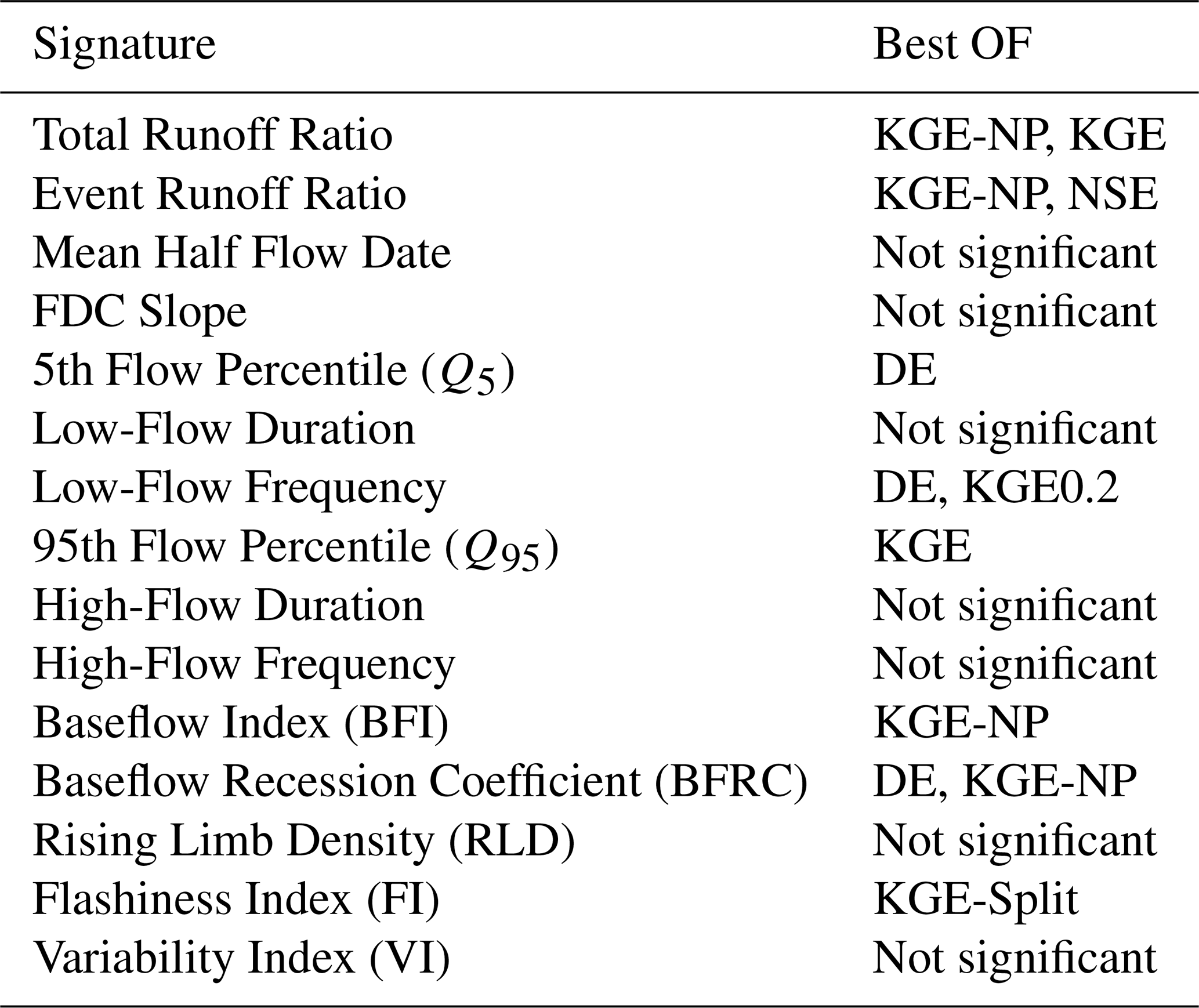
For the signatures that were found to be significantly impacted by OF choice, we used our results to develop guidelines for which OF will perform well in reproducing a given signature as shown in Table 6. We can conclude that most OF lead to the best representation for at least one signature, highlighting the need for appropriate selection. However, if the goal is a balanced representation of the water-balance and variability across hydrologic regimes, KGE-NP is a strong option. If low flows are central (ecological flows, drought assessment), preference should be given to DE or KGE0.2. If peak flows are the priority (flood risk, infrastructure design), KGE generally performs best for Q₉₅ and related high-flow signatures. Reflecting back on our review of metric choice justification (Fig. 1), we strongly recommend to document the trade-offs one is willing to accept explicitly (e.g., low-flow degradation under KGE) and, where possible, to verify unaffected signatures (e.g., MHFD, RLD) since OF changes have limited influence there.

4.2 Impact of Signature Correlations

Signatures are not independent from each other. When investigating correlations among observed signatures (Fig. 10) we noticed three clusters with similar patterns. First, a runoff/high-flow cluster (Total RR, Event RR, and Q₉₅) shows strong positive association, linking long-term water partitioning to the reaction to events. This aligns with aridity being a primary control on mean runoff (Berghuijs et al., 2017). Second, a baseflow/storage cluster, including BFI, BFRC and FI, exhibits tight coupling (higher BFI ↔ lower BFRC and FI) and a strong relationship to low-flow frequency, reflecting how sustained baseflow suppresses low-flow events. Similar to the first cluster, this group was also sensitive to objective-function (OF) choice. Third, a variability/threshold cluster (FDC slope, HFF/LFF, low-flow duration, VI) captures distributional shape and threshold exceedance. These signatures, derived from the hydrograph, partly encode duplicate information and were mostly OF-insensitive. Several other signatures showed weak or inconsistent ties to these clusters, such as High-Flow Duration, Mean Half-Flow Date, Rising Limb Density.

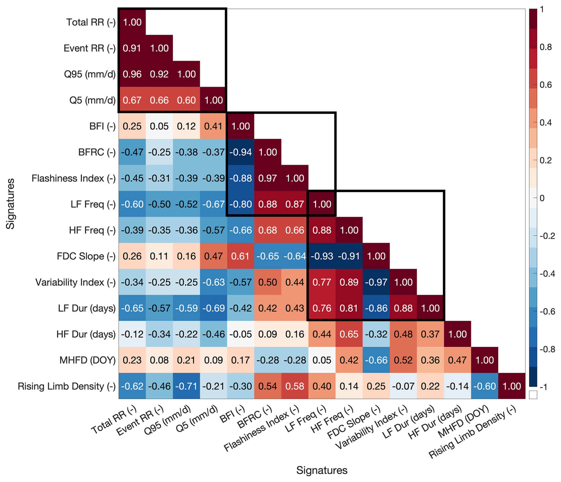
Figure 10 Correlation test between signatures based on Observations. Please note that the signatures have been reorganized in this plot to highlight the emerging patterns. Section S2.14, Fig. S35 provides a similar plot for the comparing the observed correlations to the modelled ones.

These clusters help explain why improving one signature typically also improves the other signatures in the cluster, yet they do not imply that different OFs are needed for each cluster. For example, KGE-NP performed best for many signatures in the first two clusters (e.g., Total/Event RR, BFI).

We identified some overlap between signatures that are strongly/weakly affected by OF choice and those that were identified as more/less predictable from hydrologic drivers by Addor et al. (2018): some signatures (e.g., FDC slope, durations) tend to be OF-insensitive with low spatial predictability, whereas water-balance and high-flow signatures were more OF-sensitive and spatially predictable. A notable exception is Mean Half-Flow Date, which was well predicted in Addor et al. (2018) but showed little OF sensitivity in our study suggesting a stronger climatic control.

If we consider the structural differences among OFs some of these patterns become clearer. For bias/mean terms, KGE's mean component directly constrains volumes, explaining its systematic advantage for Total RR and Q₉₅. OFs that deviate from this approach (NSE, DE, log NSE; Table 3) typically perform worse for these metrics (Gupta et al., 2009; Mizukami et al., 2019). Across objective functions, Total RR tends to be underestimated (Fig. 4), reflecting systematic water-balance biases related to excessive storage or evapotranspiration. This pattern underscores the importance of bias terms in objective functions, which directly constrain mean flow and promote a more realistic overall water balance (Mizukami et al., 2019). This underestimation is strongest for low-flow-focused objectives, as also noted by Vis et al. (2015). Our results do not support the claim that KGE resolves NSE's low-flow insensitivity or performs well simultaneously for high and low flows (Althoff and Rodrigues, 2021); note, however, that Althoff and Rodrigues (2021) investigate more basins (albeit in a specific biome), while we test a larger number of models.

For variability terms, replacing variance ratios with FDC-based components (as done for the KGE-NP) or integrating relative errors along the FDC (as done for the DE) re-targets calibration toward distributional shape and mid/low flows, improving BFI, Q₅, and Event RR in our results (Fig. 6).

For correlation terms, moving from Pearson to Spearman (KGE-NP, SHE) reduces sensitivity to extremes and stabilizes correlation. A direct comparison of KGE and SHE, where the dependence component is the only structural change, suggests improved representation for FDC slope, VI, and baseflow metrics, with similar or slightly worse performance for high-flow signatures (Kiraz et al., 2023). Annual weighting using the KGE-Split yielded mixed, context-dependent benefits and no systematic improvement of low-flow characteristics over baseline KGE in our experiments (Fig. 9; Fowler et al., 2018).

Overall, each objective function emphasizes the hydrograph component it encodes, and no single OF performs best across all signatures. Within this picture, the variability term emerges as a particularly influential lever: changes to it propagated to more signatures than changes to the correlation term, an effect most pronounced for low- and mid-flow signatures, while bias terms remain essential for water-balance and event signatures. This component-specific behaviour is consistent with evidence that signature performance depends strongly on which aspect of the hydrograph a metric targets (Mizukami et al., 2019; Melsen et al., 2019), and reinforces that OF selection should be guided by the signatures of interest rather than by a search for a universally optimal metric.

Streamflow transformations act as a further handle on signature representation, operating not on a single component but on the flow values entering all three. By compressing the dynamic range, the power and log transformations (KGE0.2, log NSE) shift calibration emphasis toward low and mid flows, which is reflected in their improved Q₅ and LFF representation at the expense of high-flow and water-balance signatures (Fig. 6). The choice and strength of transformation is therefore itself a design decision shaping which signatures a calibration favours, complementing the component-level differences discussed above (Thirel et al., 2024).

4.3 Limitations and Further Research

Our study aimed to fill a specific research gap in the current understanding of the impact of objective function choice on signature representation; using a larger number of models across diverse hydrological regimes (in comparison to Table 1). To enable a thorough investigation of the results we necessarily had to impose certain limits in other parts of the experimental design (i.e., having to “balance depth with breadth”, Gupta et al. (2014)).

First, compared to most studies in Table 1 we use a limited number of catchments. This keeps computational cost manageable and allows more detailed analysis into individual modelling results than would otherwise be possible. We selected these basins to ensure a hydro-climatic spread, as is common practice in these scenarios (see for example the 12 MOPEX basins that have been used for a large number of studies (e.g. Duan et al., 2006; van Werkhoven et al., 2008; Carrillo et al., 2011). Compared to existing studies, our selected number of objective functions and signatures is fairly typical, while our number of models is clearly higher. The presented study found relevant differences in signature representation depending on the model structure, which might indicate a limitation in generalising signature influence from single-model studies. Conversely, our broader model sample implies that conclusions drawn from the many-basin, single-model studies in Table 1 may themselves be difficult to transfer to other model structures, given that we find model choice to be a non-negligible, signature-dependent control.

Second, we focus on single-objective calibration because of its prevalence in the current literature. When multiple aspects of the flow regime matter simultaneously, multi-objective calibration has been shown to provide considerable benefits (Hernandez-Suarez et al., 2018; Nemri and Kinnard, 2020). Multi-objective formulations can expose the trade-offs explicitly via a Pareto front and allow practitioners to choose solutions that best satisfy competing goals (Yapo et al., 1998; Efstratiadis and Koutsoyiannis, 2010; Mai, 2023). If a single composite metric must be used, a transparent weighting that reflects decision priorities can be helpful. Vis et al. (2015), for instance, argue for directly incorporating multiple ecological-flow characteristics in the OF to improve the relevance of the model for management applications. Similarly, signature values have directly been used in calibration, either as additional objectives or as constraints, to target process realism (Gupta et al., 2008; Yilmaz et al., 2008; Wagener and Montanari, 2011; Euser et al., 2013; Pool et al., 2017), and our component-level insights into individual metric strengths and weaknesses can help identify which signatures or complementary metrics to add when a particular aspect of the flow regime is the target. This can potentially improve baseflow behaviour, low-flow frequency, or water-balance partitioning when those aspects are central. However, incorporating signatures does not guarantee a better hindcast/forecast skill in all settings, and can even degrade time-series fit if misapplied (Araya et al., 2023).

Third, we note the following three methodological limitations in our study design: (1) The application of the median to calculate representative values within the error metric is an important choice, as this does not capture information on the spread of the signature representation. We accounted for that by visually inspecting the underlying violins, but did not explicitly quantify the spread within the applied metrics. (2) The random-forest importance scores should be read as a relative diagnostic within this specific design rather than a universal attribution of variance. The three predictors differ in cardinality (47 models, 10 catchments, 8 objective functions), which can affect permutation-based importance, and benchmark filtering removes poorly performing combinations beforehand. The scores therefore reflect experiment-specific influence rather than general rankings of hydrological controls. (3) Finally, we did not perform any sensitivity analysis before calibrating the models, and simply calibrated all model parameters. Across all calibration runs, approximately 10 % of parameters reached one of their bounds. We found no indication that these boundary hits were systematically concentrated in a specific catchment, model, or objective function. Still, boundary hits can indicate parameter insensitivity, missing processes, data issues, or overly restrictive parameter ranges. They are therefore difficult to interpret in large multi-model calibration experiments and should be considered as an additional diagnostic of calibration reliability in future benchmarking studies.

Going forward, we see four priorities to build on the individual strengths of existing work (Table 1). First, broaden external validity with a larger, stratified basin sample (including ephemeral and groundwater-dominated systems) and potentially a wider model palette spanning physically-based and machine-learning models. Second, test cluster-aware multi-objective calibration that deliberately pairs complementary OFs, e.g., a water-balance/high-flow metric (KGE or KGE-NP) with a low-flow/storage metric (DE or KGE0.2), optionally adding signature-based components. Third, make component-level experiments less ambiguous by swapping KGE-type components one-by-one in a controlled setup, and test weighted KGE-type variants. Finally, propagate forcing/observation and signature-method uncertainty (e.g., baseflow separation) and explore information-rich objectives that go beyond the bias-variability-correlation trio, such as distributional divergences along the flow-duration curve to link calibration more directly to hydrologic processes (Kirchner, 2006). Designs like KGE-NP already go in this direction and offer a principled path to retain low-flow sensitivity without relying solely on log transforms.

5 Conclusions

We calibrated 47 conceptual model structures across 10 hydro-climatically diverse basins using 8 objective functions and evaluated how well the top-500 parameter sets for each model simulate 15 streamflow signatures. Three results stand out. First, OF choice exerts a selective influence: 8 of 15 tested signatures are OF-sensitive, while others (e.g. mean half-flow date and rising-limb density, and often event durations) change only marginally with OF choice. Second, no single OF performs best across all signatures; aggregated across OF-sensitive signatures, KGE-NP yields the smallest overall error across signatures. Third, differences are interpretable from OF design: metrics emphasizing mean volumes favour water balance and high flows; FDC-based and rank-based terms improve storage/low-flow behaviour. These patterns translate into simple steps for guiding OF choice. For accurate water balance and high-flow magnitude, KGE (or KGE-NP if distributional shape matters) is effective. When low flows and storage-related signatures are central, DE or KGE0.2 should be preferred.

While catchment differences dominate the signature values produced, it is the analysis of signature errors that matters for our purpose, since it is unsurprising that geography largely sets observed signature values. When attributing the error in reproducing each signature, the choice of objective function and model structure rise in importance, typically with OF more influential than model structure. Model structure nonetheless exerts a non-negligible, signature-dependent control on this error, particularly for low-flow and baseflow signatures, implying that findings from single-model studies cannot be assumed to generalise easily. Our findings are still bounded by the selected basins, conceptual structures, signatures, and calibration procedure but our use of 47 different models reduces that ambiguity. Priorities for future work include more systematic testing and/or multi-objective formulations, as well as broader regime and model structure coverage.

Multiple studies have indicated that OF choice is important for representing hydrologic signatures. Although process-oriented calibration may ultimately benefit most from multi-objective formulations, current practice still often relies on single-metric objective functions. For guidance on process-based modelling efforts, our study provides insights on the impact and limitations of objective function choice in a diverse selection of catchments, conceptual models and selected signatures. This is both useful as a validation approach for existing studies and guidance for further endeavours. Understanding the trade-offs in metric selection offers a practical path to models that reproduce the signatures that matter for the question at hand.