Enhancing runoff-infiltration partitioning in the SVS land surface model improves streamflow simulations under frozen soil conditions

Soil freezing is a major cold region process that influences hydrological response of northern catchments, in particular during winter rainfall and snowmelt events. In land surface models, frozen soil infiltration is difficult to represent because soil structure and hydropedological processes vary at scales finer than the model grid. This is particularly true in operational modeling, where physical process integration must balance performance improvements against computational efficiency and complexity. In this study, we propose a new configuration of the Soil, Vegetation, and Snow (SVS) model used within the operational prediction systems of Environment and Climate Change Canada (ECCC) that enhances frozen soil infiltration by reducing both surface runoff and sub-surface lateral flow. We assessed the effects of this new configuration (Fr-Inf) on streamflow simulations at more than 580 hydrometric stations located in the Great-Lakes and Saint-Lawrence domain over a five-year period. Fr-Inf significantly improves the Kling-Gupta Efficiency (KGE) compared to the default soil freezing configuration (Fr; ΔKGE = 0.28) but slightly underperforms the configuration of SVS without frozen soil (noFr; ΔKGE = −0.07). Strong degradations relative to the no freezing configuration (ΔKGE < −0.5) are observed only at 4 stations with Fr-Inf (< 1 %) as opposed to 172 stations under the Fr configuration (33 %), highlighting the robustness of the approach. To ensure that the proposed change is also acceptable in the context of operational numerical weather prediction, an evaluation of its impact on soil freezing depth as well as screen-level temperature and dew point temperature predictions is performed against in-situ observations. These results support the potential operational implementation of soil freezing at ECCC for numerical weather and streamflow prediction.

1 Introduction

Roughly half of the land surfaces in the Northern Hemisphere are underlain by permanent or seasonally frozen ground (Zhang et al., 2003). Soil freezing and thawing are major processes in cold regions that are expected to intensify under climate change (Henry, 2008), resulting in significant environmental impacts. Freeze-thaw cycles release greenhouse gases into the atmosphere, amplifying global warming through a positive climate feedback loop (Liu et al., 2024; Wang et al., 2025). Soil freezing and thawing also degrades nutrient cycling by increasing carbon and nitrogen leaching (Campbell et al., 2014; Patel et al., 2018). In terms of hydrology, several floods in cold regions occurred during snowmelt under frozen soil conditions (Barredo, 2007; Neri et al., 2019; Perry, 2000). However, the extent to which soil freezing influences a catchment response to snowmelt and rainfall remains unclear (Ala-Aho et al., 2021; Swenson et al., 2012).

At the soil sample scale, the presence of ground ice prior to snowmelt reduces soil permeability, which limits connectivity between surface and subsurface water, thereby reducing infiltration (Appels et al., 2018; Covino, 2017; Gray et al., 1985). However, this does not necessarily result in a greater runoff at larger scales. According to Wei et al. (2019), the number of freeze-thaw cycles only increases runoff when the initial soil moisture content is low, as demonstrated through a plot-scale experiment in the central US. Shanley and Chalmers (1999) conducted field experiments in northeastern US and observed a correlation between runoff and soil freezing only in a small agricultural plot (< 1 km²) but not in a larger catchment (> 100 km²). Based on multiple-year experiments in a forested catchment smaller than 20 km² located in northern Sweden, Lindström et al. (2002) found that soil freezing has no significant influence on runoff, noting that snowmelt mostly occurred after the ground had already thawed. Similarly, Stähli (2017) found no significant relationship between soil freezing and winter runoff in small Swiss subalpine catchments (< 20 km²). Although that study did not explicitly identify the underlying mechanisms, the author suggested that shallow frost depths and small-scale spatial variability in topography, vegetation, snow, and soil provide permeable areas where liquid water can infiltrate frozen ground. Studies dedicated to understanding these processes suggested that small-scale heterogeneity in soil structure along with a high initial soil moisture promote rapid infiltration into frozen soil (Stähli et al., 1999; Demand et al., 2019; Bauer et al., 2026). However, most hydrological models neglect subgrid hydropedological processes and solely rely on a single-domain matrix flow regime to represent frozen ground infiltration, which often leads to inaccurate simulations (Mohammed et al., 2018, 2021).

Typically, water flow in frozen soil is simulated by combining a water transport model, usually the Richards equation, with a heat transfer model (Dall'Amico et al., 2011; Flerchinger and Saxton, 1989; Koren et al., 1999; Zhao and Gray, 1997). The Clapeyron equation is often used to derive a soil freezing curve from a soil moisture curve (Kurylyk and Watanabe, 2013). This is done by assuming that the residual liquid water content decreases with increasing negative temperature in the same way that soil moisture decreases with increasing negative pressure (Miller, 1980). However, this method is computationally intensive because it requires solving coupled nonlinear systems. Simpler models estimate phase change using linear heat conduction algorithms between adjacent soil layers (Hayashi et al., 2007; Mohammed et al., 2013) or include a simplified solution of Stefan's equation (Changwei and Gough, 2013; Krogh et al., 2017; Krogh and Pomeroy, 2021). Still, these methods ignore convective heat exchanges and do not consider the freezing point depression caused by high negative pore pressure (Zhang et al., 2022).

To account for the formation of ice in the porous space and the resulting decrease in soil hydraulic conductivity (Burt and Williams, 1976; Harlan, 1973), numerous models use an empirical impedance factor when ice partially occupies pore space (Ganji et al., 2017; Hansson et al., 2005; Lundin, 1990; Mao et al., 2007; Smirnova et al., 2000; Taylor and Luthin, 1978). In most of these models, flow impedance increases with ice content following a power law function (Jame and Norum, 1980), which strongly limits frozen zone permeability and infiltration capacity (Kurylyk and Watanabe, 2013; Watanabe, 2008). Several models have successfully accounted for frozen ground infiltration by simulating soil water transport through a dual approach of varying complexity: a high-flow regime (preferential flow) and a low-flow regime (matrix flow) (Agnihotri et al., 2023; Larsbo et al., 2005; Šimůnek et al., 2003; Stähli et al., 1996; Weigert and Schmidt, 2005). However, integrating such approaches into land surface schemes (LSS) is often impractical due to the inherent challenges of upscaling subgrid processes, like infiltration, to a large regional scale (Vereecken et al., 2019).

This is especially true for real-time hydro-meteorological forecasting where one must generally make tradeoffs on model complexity to achieve improvements in forecast skill while meeting constraints on computing resources cost and timeliness of the forecasts. In this context, Environment and Climate Change Canada (ECCC) adheres to the same principles as the European Centre for Medium-range Weather Forecasts (ECMWF): only add complexity if there is a route to successfully initialize and verify that the forecasts are timely, skillful, relevant to users and impactful (Boussetta et al., 2021). The Soil, Vegetation and Snow (SVS; Alavi et al., 2016; Husain et al., 2016; Leonardini et al., 2020, 2021) LSS developed at ECCC and designed for operational weather and water forecasting thus falls into a category of intermediate complexity. SVS relies on simple, yet physically-based, parameterizations of surface physical processes, with the capacity to be integrated in both numerical weather prediction and hydrologic forecasting systems.

SVS simulates vertical flow between soil layers using a single domain approach, assuming that unsaturated Darcian flow is the only mechanism by which water is conveyed (Soulis et al., 2000, Alavi et al., 2016). The soil freezing scheme from the Versatile Soil Budget Model (VSBM; Mohammed et al., 2013) based on the simple heat-conduction algorithm from Hayashi et al. (2007) has recently been implemented into SVS to represent phase changes in the soil column (Amani et al., 2025). The soil freezing module of SVS accounts for the reduction of the porous space due to ice and invokes the same impedance factor as computed in the CLASS LSS to limit infiltration when soil ice is simulated (Ganji et al., 2017). However, at the time of writing, soil freezing and thawing in SVS is not yet activated in ECCC's operational forecasting systems as it generally leads to unrealistic predictions of spring freshets, as mentioned in Gaborit et al. (2025).

The main objective of this work is to improve streamflow prediction under frozen soil conditions by adjusting the existing soil infiltration configuration of the SVS LSS. The hydrological impact of this proposed configuration is assessed against the default SVS infiltration configuration, with and without soil freezing enabled, through a multi-year evaluation over a large domain that encompasses watersheds in the eastern US and Canada. Improving frozen soil infiltration in SVS would allow the activation of soil freezing and thawing processes within the operational framework of ECCC.

2 Material and methods

2.1 Code description

2.1.1 Soil water balance in SVS

ECCC uses the GEM-Hydro hydrometeorological modelling platform (Gaborit et al., 2017; Vionnet et al., 2020) within the National Surface and River Prediction System (NSRPS). The NSRPS aims to provide the most accurate real-time surface and hydrologic analyses and forecasts for Canadian and Canada/US transboundary watersheds while maintaining the quality of surface weather forecasts (Durnford et al., 2021). GEM-Hydro combines two main components: GEM-Surf, which simulates processes at the surface (Bernier et al., 2011) and Watroute for river routing (Kouwen, 2010).

GEM-surf divides each continental surface grid cell into multiple tiles and relies on SVS to represent vegetated areas and bare ground within each grid cell (Alavi et al., 2016; Husain et al., 2016; Leonardini et al., 2021). In SVS, the energy budget between the surface and the atmosphere is computed independently for four types of land surfaces: snow-free bare ground; snow-free low and high vegetation; snow over bare ground and low vegetation; and snow below high vegetation. The evolution of snow, vegetation, and bare ground surface temperatures is estimated using respective force-restore schemes (Husain et al., 2016; Leonardini et al., 2021). SVS also simulates soil hydrology as a single column of multiple layers solving 1-D Richards equations for unsaturated Darcian flow (Alavi et al., 2016).

Precipitation and snowmelt that reach the ground surface can exit the grid cell as surface runoff or infiltrate into the upper soil layer. Surface runoff (ROF; in m s⁻¹) occurs when the vertical influx rate (VI; in m s⁻¹) exceeds the vertical hydraulic conductivity of the upper soil layer ($K_{\mathrm{sat},\mathrm{v},\mathrm{1}};$ in m s⁻¹), or when a portion of this layer becomes saturated:

$$\begin{array}{}\text{(1)}& \mathrm{ROF}=\left(\mathrm{1}-{\mathrm{sat}}_{\mathrm{sfc}}\right)\max \left(\mathrm{VI}-K_{\mathrm{sat},\mathrm{v},\mathrm{1}},\mathrm{0.0}\right)+{\mathrm{sat}}_{\mathrm{sfc}}\mathrm{VI}\end{array}$$

where sat_sfc is the saturated fraction of the surface which exceeds 0 only when the soil moisture (W; unitless) of the surface layer exceeds saturation. This subgrid-scale variable is dependent on the pore size distribution and bulk saturation of the first layer (Alavi et al., 2016; Soulis et al., 2011). Water that infiltrates into the soil column can be conveyed to the layers below using a finite difference solution of the one-dimensional Richards equation, or it can exit the column as lateral flow based on the interflow calculation described in Soulis et al. (2011). This approach relies on the exceedance of the field capacity (W_fc; unitless) of any i soil layer:

$$\begin{array}{}\text{(2)}& W_{\mathrm{fc},i}={\displaystyle \frac{W_{\mathrm{sat},i}}{b-\mathrm{1}}}{\left(-{\displaystyle \frac{{\mathit{\psi }}_{\mathrm{sat},i}b}{\mathrm{2}{D}_{\mathrm{d}}s}}\right)}^{\mathrm{1}/b}\left({\left(\mathrm{3}b+\mathrm{2}\right)}^{(b-\mathrm{1})/b}-{\left(\mathrm{2}b+\mathrm{2}\right)}^{(b-\mathrm{1})/b}\right)\end{array}$$

where the saturated water content, W_sat (unitless), the saturated soil matric potential, ψ_sat (m), and the slope of the water retention curve from Clapp and Hornberger (1978), b (unitless), are all soil texture-dependent parameters:

$$\begin{array}{}\text{(3)}& {\displaystyle }{W}_{\mathrm{sat}}=-\mathrm{0.00126}{X}_{\mathrm{sand}}+\mathrm{0.489}\text{(4)}& {\displaystyle }{\mathit{\psi }}_{\mathrm{sat}}={\displaystyle \frac{{\mathrm{10}}^{\left(-\mathrm{0.0131}{X}_{\mathrm{sand}}+\mathrm{1.88}\right)}}{\mathrm{100}}}\text{(5)}& {\displaystyle }b=\mathrm{0.137}{X}_{\mathrm{clay}}+\mathrm{3.501}\end{array}$$

with X_sand and X_clay being the sand and clay percentages (between 0 and 100) of any soil layer, respectively. In Eq. (2), 2D_ds corresponds to the tile slope-to-length ratio with D_d and s being the drainage density (in m m⁻²) and the slope (in m m⁻¹) of the tile, respectively. The slope-to-length ratio is then applied to the horizontal hydraulic conductivity (K_sat,h; in m s⁻¹) to modulate the interflow. Additionally, K_sat,h depends on K_sat,v and decays with depth, favoring lateral flow for layers near the surface:

$$\begin{array}{}\text{(6)}& K_{\mathrm{sat},\mathrm{h}}=a{K}_{\mathrm{sat},\mathrm{v}}\exp \left[c{\displaystyle \frac{D-d}{D}}\right]\end{array}$$

where D (m) is the depth of the whole soil column while d (m) is the depth of the soil layer, and a and c are anisotropic constants (a = 10 and c = 5). Lateral flow also occurs when there is insufficient space in the underlying layer to receive the excess water of a given i soil layer:

$$\begin{array}{}\text{(7)}& \begin{array}{rl}\mathrm{LAT}& =\max \left(\right(W_i-W_{\mathrm{sat},i})\mathrm{\Delta }{d}_i\\ & -(W_{i+\mathrm{1}}-W_{\mathrm{sat},i+\mathrm{1}})\mathrm{\Delta }{d}_{i+\mathrm{1}},\mathrm{0.0})\end{array}\end{array}$$

where LAT is the lateral flow (m) and Δd (m) corresponds the thickness of each layer. LAT is cumulated over each calculation timestep and converted in m s⁻¹. By configuration, this mechanism does not generate lateral flow in the last soil layer. Instead, water that reaches the deepest soil layer (denoted N) leaves the soil column as drainage when the field capacity of this layer is exceeded. The field capacity of the deepest soil layer is computed using Eq. (2) adjusted to account for total soil depth (Soulis et al., 2011):

$$\begin{array}{}\text{(8)}& W_{\mathrm{fc},N}={\displaystyle \frac{W_{\mathrm{sat},N}}{b-\mathrm{1}}}{\left({\displaystyle \frac{{\mathit{\psi }}_{\mathrm{sat},N}b}{D}}\right)}^{\mathrm{1}/b}\left({\left(\mathrm{3}b+\mathrm{2}\right)}^{(b-\mathrm{1})/b}-{\left(\mathrm{2}b+\mathrm{2}\right)}^{(b-\mathrm{1})/b}\right).\end{array}$$

Within GEM-Surf, SVS includes an optional, non-explicit representation of the effects of tile drains and ploughing in agricultural areas (Gaborit et al., 2025). For simulating the effect of tile drains, a multiplicative coefficient, m_h, is applied to the K_sat,h of the fifth soil layer (between 40 and 100 cm deep), which is further weighted by the fraction of agricultural cover in the land tile of the grid-cell. This results in an increase in lateral flow. Similarly, the effect of ploughing is modeled by applying a multiplicative factor, m_v, to the vertical hydraulic conductivity K_sat,v of the first three soil layers (between the surface and 20 cm deep), which increases vertical water transport near the surface. In our study, the multiplicative factors for the effect of tile drains and ploughing were set to 500 for m_h and 10 for m_v. These values are based on the calibration work performed by Gaborit et al. (2025) and allow to promote greater lateral flow in agricultural catchments. Figure 1a provides a conceptual overview of the soil water fluxes in the default version of SVS without soil freezing.

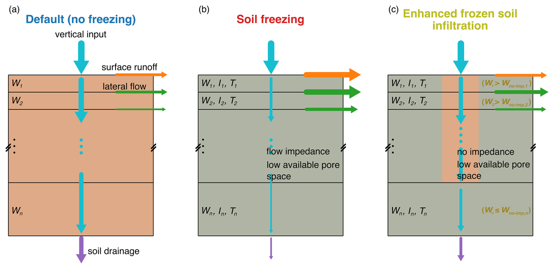
Figure 1 Conceptual scheme of the soil water balance in SVS (evapotranspiration is not shown here) for (a) the default configuration without soil freezing, (b) the soil freezing configuration and (c) the configuration of enhanced frozen ground infiltration. W denotes the water content of layer i while I and T denote the ice fraction and the temperature of layer i, respectively, on (b) and (c). Vertical downward water flux through the soil column is shown by blue arrows while orange, green and purple arrows correspond to surface runoff, lateral flow and soil drainage, respectively. The relative size of the arrows represents the relative magnitude of the fluxes in each configuration.

Watroute (Kouwen, 2010) is a gridded routing scheme that conveys water through a network of rivers and lakes to simulate streamflow and water levels. The version used at ECCC can explicitly represent diversions, lakes and reservoirs, using the dynamically zoned target release model for the latter (Gaborit et al., 2022; Yassin et al., 2019). Surface runoff and lateral flow from GEM-Surf contribute directly to the surface network in Watroute. In contrast, soil drainage is added to the lower zone storage of Watroute, which is a conceptual reservoir used to represent aquifers and simulate baseflow, which is then also provided to the surface network in Watroute.

2.1.2 Soil freezing module

The version of SVS used in GEM-Surf includes an optional representation of soil freeze/thaw processes which is described in Amani et al. (2025). The following section provides a summary of the soil freezing module in SVS, emphasizing new additions to the module.

The soil freezing module relies on a simple heat-conduction algorithm (Hayashi et al., 2007) described in the VSBM model (Mohammed et al., 2013). This approach estimates the temperature and phase changes for each soil layer and uses the upper boundary condition provided by force-restore schemes. Compared to the iterative solutions of coupled nonlinear equations, this approach is less computationally intensive and suits the level of complexity of the force-restore schemes used for the surface energy balance in SVS.

The heat conduction algorithm in SVS assumes that the change in net heat flux for any given layer corresponds to the change in stored latent and sensible heat and is calculated sequentially from top to bottom within the soil column. This simple approach ignores the freezing-point depression and water in soil pores is assumed to freeze at T_ref = 273.15 K (Kurylyk and Watanabe, 2013). However, liquid water can remain at sub-zero temperatures and coexist with ice. When the soil layer temperature is not equal to T_ref (i.e. when the layer is completely thawed or frozen), the change in net heat flux converts into sensible heat until the soil layer temperature reaches T_ref. When the soil layer temperature equals T_ref, the change in net heat flux is first used for melting or freezing all available water above the residual unfrozen water content, converting any residual energy into sensible heat.

The residual unfrozen water content depends on soil texture and saturated water content based on Niu and Yang (2006). Their model allows to derive the maximum unfrozen water content as a function of soil texture and temperature. However, since SVS assumes that phase change only occurs at 273.15 K, a unique residual unfrozen water content is associated to any given soil texture, regardless of soil temperature under frozen conditions. It corresponds to the average of the values obtained from Eq. (3) of Niu and Yang (2006) for soil temperatures (T_i) from 263.15 to 275.15 K by increments of 2 K:

$$\begin{array}{}\text{(9)}& W_{\mathrm{res}}={\displaystyle \frac{W_{\mathrm{sat}}{\sum }_{i=\mathrm{1}}^{n=\mathrm{5}}{\left[\frac{{\mathrm{10}}^{\mathrm{3}}{L}_{\mathrm{f}}\left(T_i-T_{\mathrm{ref}}\right)}{g{T}_i{\mathit{\psi }}_{\mathrm{sat}}}\right]}^{-\mathrm{1}/b}}{n}}\end{array}$$

where L_f and g are the latent heat of fusion (334 J kg⁻¹) and the gravitational constant (9.81 m s⁻²), respectively.

For phase change computation, we apply an efficiency factor based on the soil water content of each layer similar to that used in the ISBA model (Boone et al., 2000):

$$\begin{array}{}\text{(10a)}& {\displaystyle }{\mathit{\chi }}_{\mathrm{fr}}=\left(W-W_{\mathrm{res}}\right)/W_{\mathrm{sat}}\text{(10b)}& {\displaystyle }{\mathit{\chi }}_{\mathrm{th}}=I/\left(W_{\mathrm{sat}}-W_{\mathrm{res}}\right)\end{array}$$

where χ_fr and χ_th are respectively the efficiency factors for freezing and thawing (unitless), W is the soil moisture and I is the volumetric ice fraction, both unitless. This approach implies that a given soil layer with high soil moisture (ice) content freezes (thaws) more rapidly than when it contains less liquid water (ice)(Pitman et al., 1991). The minimal value that χ_fr and χ_th can take was set to 0.6.

The lower boundary condition for temperature is set at a depth of 2.5 times the total thickness of the soil column. For a typical SVS soil configuration of a 3 m depth, this corresponds to a depth of 7.5 m. This approach aims to minimize the error in both soil water and energy budgets (Decharme et al., 2013). The upper boundary condition is the sum of the heat fluxes from each of the four surface energy budgets (see Sect. 2.1.1), weighted by their respective fractions. For bare ground, the heat flux varies according to the difference between the skin temperature from the soil force-restore scheme and the temperature of the surface soil layer. Recent improvements in the soil freezing scheme of SVS make that the release and absorption of latent heat due to soil freezing and thawing now impact the evolution of the temperature variables of the bare ground in the force-restore scheme as follows:

$$\begin{array}{}\text{(11)}& \mathrm{\Delta }{T}_{\mathrm{grnd},j}={\mathit{\chi }}_j{L}_f{C}_g\mathrm{\Delta }{W}_{\mathrm{LH}}\end{array}$$

where ΔT_grnd,j is the gain (loss) of surface or deep bare ground temperature (in K) in the force-restore scheme associated to the release (absorption) of mass from the latent heat flux (ΔW_LH; in kg m⁻²). χ_j corresponds to the efficiency factor for freezing in the case of latent heat release (ΔT_grnd,j positive) and for melting, inversely. C_g is the soil thermal coefficient for the force-restore scheme (in K m⁻² J⁻¹) based on soil porosity and texture, and on water and ice content for the topmost soil layer. The latent heat flux from the upper 5 cm is considered for ΔT_grnd,surf while the latent heat flux of soil layers between 5 and 100 cm deep is used for ΔT_grnd,deep.

For snow-free vegetation (low and high), a constant skin conductivity of 10 W K⁻¹ m⁻² is applied to the difference between the vegetation skin temperature and the temperature of the upper soil layer for estimating the heat flux (Boussetta et al., 2021). For bare ground, a constant skin conductivity of 15 W K⁻¹ m⁻² is used. The heat flux between the ground and the snowpack depends on the snow thermal conductivity and on the difference between the deep snow temperature from the force-restore scheme and the surface layer temperature, if the snow depth is greater than the thermal damping depth. Otherwise, the skin snow temperature is used instead. Equations used for the snow thermal conductivity, and the thermal damping depth are presented in Leonardini et al. (2021). The fraction of the tile covered by snow is estimated using the configuration from Niu and Yang (2007).

The soil freezing module directly impacts soil hydrology. First, available pore space decreases as the ice fraction increases, reducing the available space for liquid water (Zhao and Gray, 1997):

$$\begin{array}{}\text{(12)}& W_{\mathrm{sat},\mathrm{fr}}=W_{\mathrm{sat}}-I\end{array}$$

where W_sat,fr is the saturated water content (unitless) adjusted for the presence of soil ice.

Second, the presence of ground ice decreases the K_sat,v through an impedance factor, described as follows (Ganji et al., 2017):

$$\begin{array}{}\text{(13)}& K_{\mathrm{sat},\mathrm{v},\mathrm{fr}}={\left[\mathrm{1}-\min \left(\mathrm{1.0},{\displaystyle \frac{I}{W_{\mathrm{sat}}}}\right)\right]}^{\mathrm{2}}{K}_{\mathrm{sat},\mathrm{v}}\end{array}$$

where $K_{\mathrm{sat},\mathrm{v},\mathrm{fr}}$ (m s⁻¹) is the hydraulic conductivity of the soil layer when it is partially frozen.

Overall, growing soil ice has to major impact on the soil water balance. First, it reduces the saturated water content which makes the saturation of the soil layers more likely (Eq. 7) and the exceedance of field capacity easier (Eq. 2) for lateral flow generation. Second, it reduces the vertical hydraulic conductivity, favoring even more soil saturation and surface runoff (Eq. 1). These effects are shown in conceptual Fig. 1b.

2.1.3 Enhanced frozen soil infiltration

Enhancement of infiltration under frozen soil conditions into SVS relies on a conceptual relaxation of ice impedance based on soil moisture and on a structural modification of surface runoff generation. First, we implemented a condition that verifies if the liquid water content of each soil layer at any given timestep exceeds a no-impedance threshold (W_no-imp, unitless):

$$\begin{array}{}\text{(14)}& W_{\text{no-imp}}={\mathit{\alpha }}_{\text{no-imp}}{W}_{\mathrm{sat},\mathrm{fr}}\end{array}$$

where α_no-imp is a static calibrated parameter between 0 and 1 representing the fraction of saturated water content to be considered for removing ice-impedance. We chose a dependency on soil moisture since the routine for water diffusion in unsaturated porous media from Soulis et al. (2000) used in SVS resolves Richards equation based on the water content (Alavi et al., 2016). In the configuration proposed here, when W exceeds W_no-imp, the vertical hydraulic conductivity of frozen soil ($K_{\mathrm{sat},\mathrm{v},\mathrm{fr}}$) corresponds to that of an unfrozen soil (K_sat,v). Thus, when the soil is completely unfrozen and W>W_no-imp, there is no effect on the soil hydraulic conductivity. This simple conceptual approach aims to increase infiltration into frozen soils while remaining simple to implement operationally compared to other models relying on dual-domain approaches (Larsbo et al., 2005; Ross and Smettem, 2000; Šimůnek et al., 2003; Stähli et al., 1996).

Second, the enhanced frozen soil infiltration configuration includes a modification to the surface runoff generation so it only occurs when the vertical water input rate exceeds the infiltration rate. Technically, it implies that sat_sfc in Eq. (1) is set to 0. This new feature, which is activated under frozen and unfrozen soil conditions, influences runoff-infiltration partitioning when the surface soil layer approaches saturation. This seldom occurs in the absence of ice in the topmost soil layer. We decided to apply this correction also for unfrozen soil since this approach is fundamentally designed to generate interflow rather than surface runoff. Overall, the enhanced frozen soil infiltration configuration limits the decreasing effect of growing ice on soil saturation and $K_{\mathrm{sat},\mathrm{v},\mathrm{fr}}$ and corrects runoff generation formulation. This approach aims to foster infiltration under frozen soil conditions, as illustrated in Fig. 1c.

2.2 Modeling setup

The study area covers the Great-Lakes and Saint-Lawrence (GLSL) domain, which includes the five Great-Lakes watersheds (Lake Superior, Lake Michigan, Lake Huron, Lake Erie, and Lake Ontario), the Ottawa River Basin (which occupies provinces of Ontario and Québec), and the Saint-Lawrence Valley, including the Saguenay Lac-Saint-Jean watershed in the northeast of the domain (Fig. 2). The northern half of the domain is primarily forested, with a transition from deciduous to coniferous forests from south to north. Agricultural areas dominate the region between Lake Erie and Lake Huron, as well as the southwest of Lake Erie and the shores of the Saint-Lawrence Valley. The GLSL domain also includes urban areas like the Greater Toronto Area, the Montréal metropolitan area, and the US cities of Chicago, Detroit, Cleveland, and Buffalo, among others. The terrain is relatively flat in most of the Great-Lakes watersheds but becomes hillier in the northeast of the domain, which also includes part of the Appalachian mountains in the Lake Champlain watershed. Note the existence of a large, confined aquifer in southern Michigan (between Lake Michigan and Lake Huron; Lampe, 2009) and the presence of numerous wetlands in the north of Lake Michigan and in southern Ontario (Penfound and Vaz, 2022). These have an influence on streamflow regime but are not represented explicitly in GEM-Hydro (Gaborit et al., 2025).

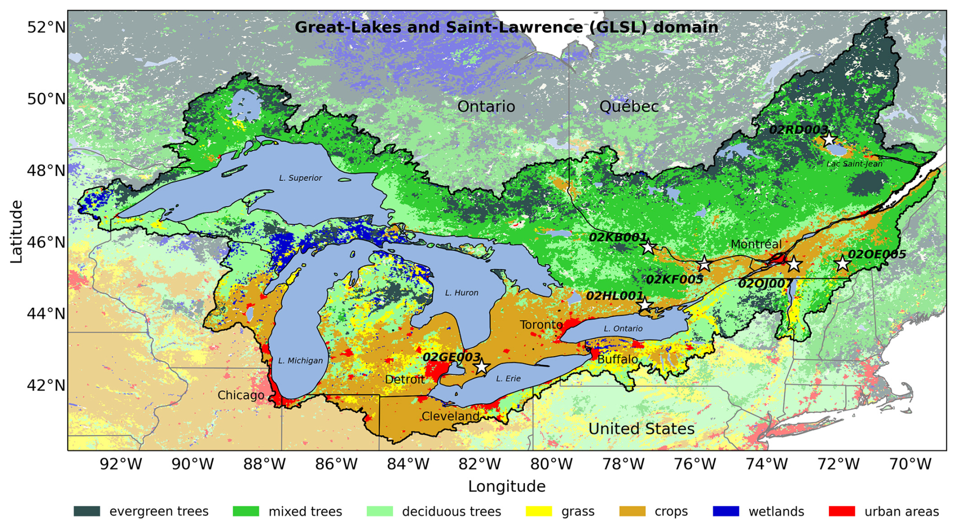
Figure 2 Map of the dominant vegetation class for each grid cell within the Great-Lakes and Saint-Lawrence (GLSL) domain. The location of the hydrometric stations used for the hydrograph analysis is identified by a white star (see Sect. 3.4).

For the evaluation, we considered three open-loop experiments with GEM-Hydro: a first experiment in which the soil freezing module of SVS is not activated (noFr), a second experiment in which the default soil freezing module is activated (Fr), and a third experiment in which the enhanced frozen soil infiltration is enabled (Fr-Inf). In all three experiments, we use the geophysical fields described by Gaborit et al. (2025) in their final GEM-Hydro setup and we set the soil column as seven soil layers extending down to three meters with increasing thickness.

We ran GEM-Surf and Watroute at spatial resolutions of 2.5 and 1 km, respectively. GEM-Hydro was forced hourly with the version 3.1 of the Canadian Surface Reanalysis (CaSRv3.1, see Gasset et al., 2025). CaSRv3.1 relies on a 10 km configuration of the GEM atmospheric model (McTaggart‐Cowan et al., 2019) which is initialized every 12 h from the ERA5 atmospheric reanalysis (Hersbach et al., 2020) and is coupled with the Canadian Land Data Assimilation System (CaLDAS, Carrera et al., 2015) and the Canadian Precipitation Analysis (CaPA; Fortin et al., 2015), which uses surface observations and optimal interpolation to produce gridded precipitation reanalysis at 24 h. The main improvements of CaSRv3.1 compared to the previous version (v2.1; Gasset et al., 2021) are the correction of a cold bias in air temperature in the spring as well as the use of ERA5 instead of ERA-Interim for initial conditions. Precipitation phase was partitioned between liquid and solid based on the near-surface wet-bulb temperature (Wang et al., 2019).

We ran each GEM-Hydro experiment from 1 September 2015 to 31 August 2021, with the first year of simulation (until 31 August 2016) used as a spinup year. Therefore, the evaluation period lasts 5 complete years from 2016 to 2021. We selected this period as it covers years of various hydrometeorological conditions in eastern North America. For instance, the water level of several of the Great Lakes reached new historical records in 2017 and 2019 (Gronewold et al., 2021). This, combined with snowmelt and heavy rainfall in spring, contributed to major flooding in several municipalities of Southern Québec (Jean et al., 2024). In contrast, the year 2020–2021 was exceptionally warm and dry in eastern Canada leading to low-flow conditions in spring (Bouchard et al., 2024; NOAA, 2021).

Note that at the time of writing, a version 3.2 of CaSR that includes a bug fix has been released (Khedhaouiria et al., 2026). However, version 3.2 of CaSR is identical to version 3.1 for our period of simulation and has no impact on surface simulations.

2.3 Calibration of the no-impedance threshold parameter

The enhanced frozen soil infiltration configuration comes with a new parameter (α_no-imp) indicating the fraction of soil moisture at saturation at which ice impedance is removed. We calibrated α_no-imp by running open-loop simulations with GEM-Hydro and using no-impedance thresholds starting from 0.5 to 0.99 by increments of 0.05 over the GLSL domain. We used the CaSRv3.1 reanalysis to force the model from 1 September 2015 to 31 August 2018 with the first complete year used as a spinup. The rest of the setup is configured the same as that mentioned in Sect. 2.2.

We set the upper boundary for the sensitivity analysis to α_no-imp = 0.99 to replicate restrictive conditions to infiltration similar to that of the default soil freezing configuration (Fr). The lower boundary of the sensitivity analysis is based on irrigation experiments and one-dimensional water flow modeling with MACRO (Stenemo and Jarvis, 2010) performed by Alaoui (2015) who suggested that the soil moisture threshold beyond which preferential flow is initiated is approximately half of the saturated water content.

2.4 Evaluation data and metrics

2.4.1 Simulated streamflow

The GLSL domain encompasses a network of hydrometric stations distributed across US and Canada. The US daily streamflow observations were retrieved from the USGS database (https://waterdata.usgs.gov/nwis/dv?referred_module=sw&search_criteria=site_tp_cd&submitted_form=introduction, last access: 27 July 2026) while the Canadian daily streamflow observations come from the HYDAT database (https://www.canada.ca/en/environment-climate-change/services/water-overview/quantity/monitoring/survey/data-products-services/national-archive-hydat.html, last access: 27 July 2026). During the evaluation period (2016–2021), streamflow observations were available for 581 stations across the domain. For the upstream catchment related to each station, we extracted the corresponding land surface types and the depth-averaged soil texture (to 3 m) from the geophysical field dataset. We evaluated the streamflow simulation performances of the three experiments based on three metrics: the relative percent bias (PBIAS), the Nash Sutcliffe Efficiency (NSE; Nash and Sutcliffe, 1970) and the Kling Gupta efficiency (KGE; Kling et al., 2012).

The PBIAS (%) can be expressed as follows:

$$\begin{array}{}\text{(15)}& \mathrm{PBIAS}=\mathrm{100}{\displaystyle \frac{{\sum }_{i=\mathrm{1}}^N\left(S_i-O_i\right)}{{\sum }_{i=\mathrm{1}}^N{O}_i}}\end{array}$$

where N is the total number of observation-simulation pairs, and S_i and O_i are the simulated and observed daily streamflow for day i (m³ s⁻¹), respectively. According to Eq. (15), a positive (negative) PBIAS denotes that the model overestimates (underestimates) the observed streamflow.

The NSE [−∞, 1] is a normalized variant of the Mean Squared Error and can be written as follows:

$$\begin{array}{}\text{(16)}& \mathrm{NSE}=\mathrm{1}-{\displaystyle \frac{{\sum }_{i=\mathrm{1}}^N{\left(S_i-O_i\right)}^{\mathrm{2}}}{{\sum }_{i=\mathrm{1}}^N{\left(O_i-\stackrel{\mathrm{‾}}{O}\right)}^{\mathrm{2}}}}\end{array}$$

where O is the mean of the observed daily streamflow. A NSE of 1 means that the simulations perfectly agree with the observations.

Finally, the KGE [−∞, 1] is one minus the Euclidean distance computed between the bias, the variability and the correlation based on their cartesian coordinates:

$$\begin{array}{}\text{(17)}& \mathrm{KGE}=\mathrm{1}-\sqrt{{\left(r-\mathrm{1}\right)}^{\mathrm{2}}+{\left({\displaystyle \frac{\stackrel{\mathrm{‾}}{S}}{\stackrel{\mathrm{‾}}{O}}}-\mathrm{1}\right)}^{\mathrm{2}}+{\left({\displaystyle \frac{{\mathrm{CV}}_{\mathrm{S}}}{{\mathrm{CV}}_{\mathrm{O}}}}-\mathrm{1}\right)}^{\mathrm{2}}}\end{array}$$

where r is the Pearson correlation coefficient, $\stackrel{\mathrm{‾}}{S}$ is the mean of the simulated streamflow (m³ s⁻¹), CV_S and CV_O are coefficients of variability of the simulated and observed daily streamflow (m³ s⁻¹), respectively. A KGE of 1 implies that the first and second statistical moments (the mean and the variance) of the observed and simulated streamflow are the same and that both samples are perfectly correlated.

When comparing two or more experiments for a given station, we decided to exclude the station from the analysis if the NSE or KGE of at least one experiment was lower than 0 and −0.41, respectively, indicating that the mean of the observations is a better predictor of streamflow than the model (see Eqs. 16 and 17 and Knoben et al., 2019). We use this approach to ensure that our analysis includes only stations for which the reference experiment (noFr or Fr) yields reasonable results or is improved by the enhancement of frozen soil infiltration.

2.4.2 Near-surface meteorological variables and freezing depth

The surface component of GEM-Hydro has been developed to be used for offline applications such as the NSRPS as well as coupled applications in the context of Numerical Weather Prediction systems. For this reason, we evaluate the impact of soil freezing (with or without enhanced infiltration) on near-surface meteorological variables: 2 m air temperature (TT, in °C) and the 2 m dew point temperature (TD; in °C). The two variables are obtained from GEM-Hydro by interpolating between values at the surface and values of the height of the CaSRv3.1 forcing level using vertical profiles derived from Monin-Obukhov stability theory. The evaluation was performed by comparing hourly model simulations to in-situ observations from METAR, SYNOP and SWOB observation networks over the whole domain. In total, this corresponds to 667 stations for the 2016–2021 evaluation period. We evaluated each experiment by computing the mean bias (BIAS), the root mean squared error (RMSE) and the standard deviation of the error (SD). Then, we computed the difference in performance between the Fr and noFr experiments and between the Fr-Inf and the noFr experiments.

The BIAS, the RMSE and the SD are computed using Eqs. (18) to (20):

$$\begin{array}{}\text{(18)}& {\displaystyle }\mathrm{BIAS}={\displaystyle \frac{\mathrm{1}}{N}}{\sum }_{i=\mathrm{1}}^N\left(S_i-O_i\right)\text{(19)}& {\displaystyle }\mathrm{RMSE}=\sqrt{{\displaystyle \frac{\mathrm{1}}{N}}{\sum }_{i=\mathrm{1}}^N{\left(S_i-O_i\right)}^{\mathrm{2}}}\text{(20)}& {\displaystyle }\mathrm{SD}=\sqrt{{\displaystyle \frac{\mathrm{1}}{N}}{\sum }_{i=\mathrm{1}}^N{\left(X_i-\stackrel{\mathrm{‾}}{X}\right)}^{\mathrm{2}}}\end{array}$$

where S_i and O_i are the simulated and observed values for either TT or TD. X_i is the difference between the modeled and observed value (S_i−O_i) for time-step i and $\stackrel{\mathrm{‾}}{X}$ is the average of the differences of all observation-simulation pairs.

The difference in BIAS, RMSE and SD between experiments is expressed as shown by Eqs. (21) to (23):

$$\begin{array}{}\text{(21)}& {\displaystyle }\mathrm{\Delta }\mathrm{BIAS}=\left|{\mathrm{BIAS}}_{\mathrm{noFr}}\right|-\left|{\mathrm{BIAS}}_{\exp }\right|\text{(22)}& {\displaystyle }\mathrm{\Delta }\mathrm{RMSE}={\mathrm{RMSE}}_{\mathrm{noFr}}-{\mathrm{RMSE}}_{\exp }\text{(23)}& {\displaystyle }\mathrm{\Delta }\mathrm{SD}={\mathrm{SD}}_{\mathrm{noFr}}-{\mathrm{SD}}_{\exp }\end{array}$$

where ΔBIAS, ΔRMSE and ΔSD are the differences in BIAS, RMSE and SD in °C while the index exp denotes either Fr or Fr-Inf experiments. The BIAS, the RMSE and the SD are in °C.

Finally, we evaluated the capacity of the Fr and Fr-Inf experiments to accurately simulate the freezing depth. We define the freezing depth (FD) as the depth of the upper boundary of the last layer in which the ice fraction is greater than zero, plus the fraction of the porous space occupied by ice in that layer, multiplied by its thickness:

$$\begin{array}{}\text{(24)}& \mathrm{FD}=z+{\displaystyle \frac{I}{\left(W_{\mathrm{sat}}-W_{\mathrm{res}}\right)}}\mathrm{\Delta }d\end{array}$$

where z and Δd (both in m) are, respectively, the depth of the upper boundary and the thickness of the deepest frozen soil layer. The modeled FD is then compared to observations retrieved from the North Central River Forecast Center database (https://www.weather.gov/ncrfc/LMI_ncrfc_forecast_products, last access: 27 July 2026), which includes manual freezing depth measurements taken at 103 locations in the central US from 2016 to 2021. The bi-monthly mean of the modeled and observed FD at all locations was computed to evaluate the model bias, RMSE and standard deviation of the error (Eqs. 18, 19 and 20).

3 Results

3.1 Hydrologic impact of the default soil freezing configuration

Figure 3 illustrates the differences in KGE between the soil freezing (Fr) and the no freezing (noFr) experiments over the Great-Lakes and Saint-Lawrence domain from 2016 to 2021. As Fig. 3 shows, incorporating soil freezing into the model without a mechanism to promote infiltration degrades streamflow simulations at 92 % of the stations, spread all over the domain (ΔKGE = −0.44). This degradation of KGE is explained by the degradation of the NSE (not shown). This occurs because the model tends to overestimate streamflow peaks in winter and spring when ground ice is simulated and infiltration is highly restricted.

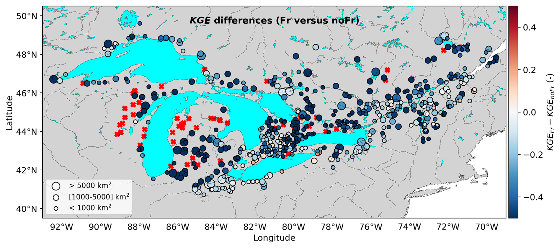
Figure 3 Map of the KGE differences between the soil freezing (Fr) experiment and the experiment without soil freezing (noFr) over the Great-Lakes and Saint-Lawrence domain for the 2016–2021 period. Degradations of the KGE with the Fr experiment (negative KGE differences) are represented by cold-colored dots. Red crosses show stations excluded from the comparison (see Sect. 2.4.1).

The KGE is degraded by more than 0.5 for 172 stations (33 %). These stations are primarily concentrated in Michigan, where the perched aquifer is present, as well as along the Niagara Escarpment between Lake Ontario and Lake Huron, where the exchange of surface and groundwater is enhanced, contributing to a larger base flow. The model does not account for these phenomena, which could further degrade its performance when combined with soil freezing configuration. This may also explain the emergence of excluded stations (red crosses) northwest of Lake Michigan and between Lakes Michigan and Huron.

Most of the stations where the Fr experiment results in a better KGE than the noFr experiment (warm-colored dots) are located in agricultural and urban areas, where reactive runoff is favored by tile drains and surface imperviousness, respectively. It is possible that soil freezing compensates for the fact the model does not explicitly represent the effect of tile drain and urban areas in some catchments, as shown by the use of larger values for m_h and m_v.

3.2 Optimization of α_no-imp

Hydrologic simulations with the enhanced frozen ground infiltration configuration (Fr-Inf), using incremental values of α_no-imp starting from 0.5, show that the KGE is the highest with the lowest α_no-imp values (Fig. 4a). The Fr-Inf performance is quite stable when α_no-imp is 0.7 or lower, with a median KGE greater than 0.5, and the fifth and ninety-fifth percentiles greater than 0.2 and 0.8, respectively. However, the performance decreases significantly for simulations with larger α_no-imp values. This suggests that the model performs better when the ice impedance effect on flow is limited. Consequently, the lowest KGE is obtained in the experiment with the most restrictive infiltration conditions (α_no-imp = 0.99). Conceptually, this experiment is similar to the default soil freezing configuration (Fr). This sensitivity analysis demonstrates that adding a simple relaxation of ice-induced flow impedance in SVS improves the KGE on the GLSL domain regardless of the value of α_no-imp.

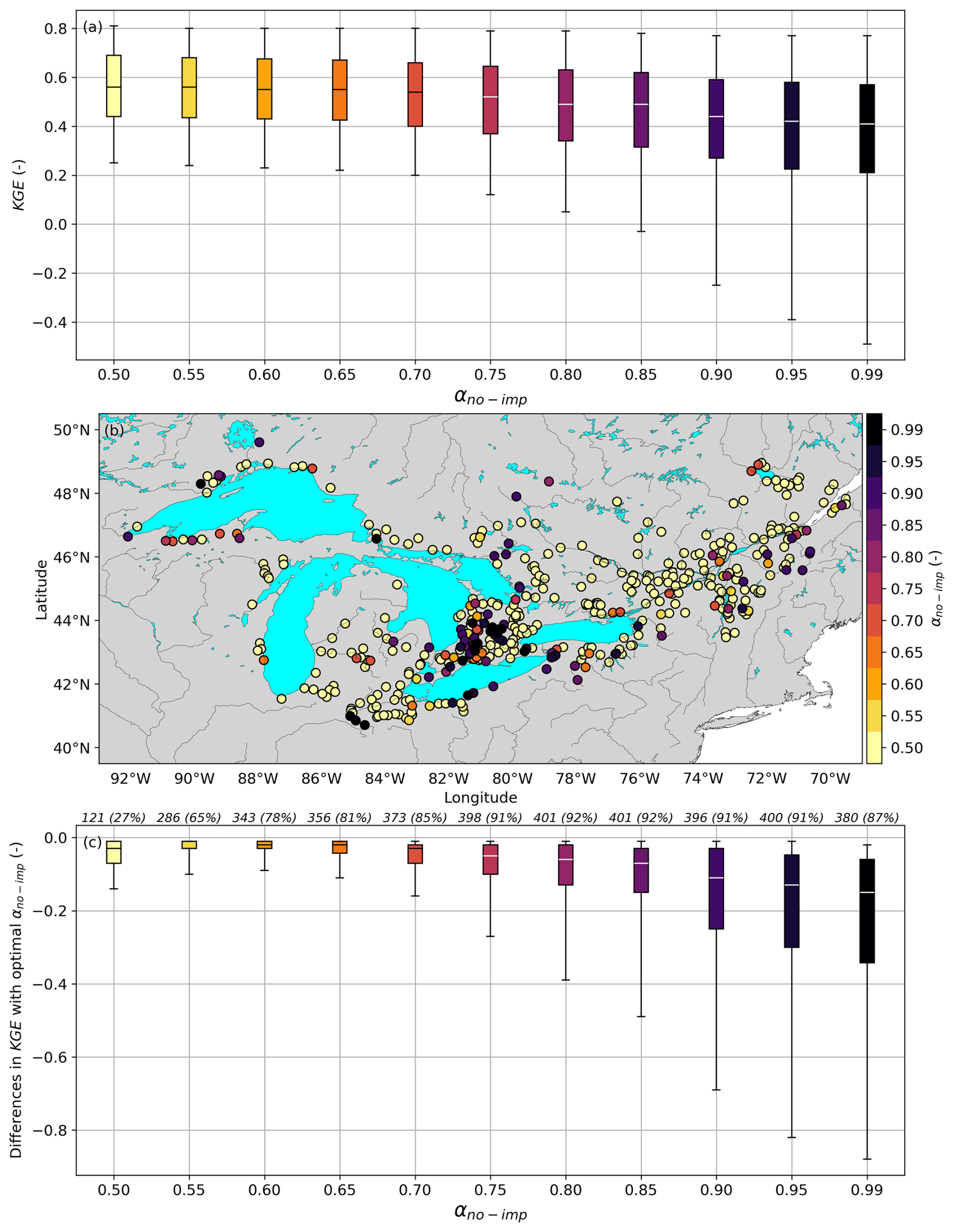
Figure 4 Boxplots of streamflow KGE for the enhanced frozen soil infiltration configuration (Fr-Inf) using values of α_no-imp from 0.50 to 0.99 by increments of 0.05 on the Great-Lakes and Saint-Lawrence domain from 1 September 2016 to 31 August 2018 (a). The target value for the KGE is 1. Map showing the value of α_no-imp which results in the best KGE for each station (b). When two experiments with different α_no-imp result in the same KGE on a given station, the experiment with the lowest α_no-imp is shown on the map. Only stations for which at least one experiment results in a NSE greater than 0 or a KGE greater than −0.41 (see Sect. 2.4.1) are shown in (a) and (b) (435 stations). Boxplots of the differences in KGE between experiments with each value of α_no-imp and the experiment resulting in the best KGE at stations for which the given experiment does not result in the best KGE (number and percentage of station shown above each boxplot) (c). The lower and upper limits of the boxes in (a) and (c) correspond to the first and third quantile, the median is shown by a horizontal black (α_no-imp = 0.50 to 0.70) or white (α_no-imp = 0.75 to 0.99) line and the lower and upper whiskers represent the fifth and ninety-fifth percentiles while the outliers are not shown.

For most stations, a value of α_no-imp of 0.5 leads to a better or equivalent KGE than larger values of α_no-imp. These values are uniformly distributed across the domain, as shown by the widely spread yellow dots in Fig. 4b. However, the optimal α_no-imp varies considerably with land surface characteristics (see Fig. S1 in the Supplement) as shown by generally larger optimal α_no-imp value in catchments of low forest fraction (0 %–20 %) and high crop fraction (80 %–100 %). Nonetheless, the optimal α_no-imp parameter exhibits greater sensitivity to soil texture. In particular, catchments for which low α_no-imp performs better are also characterized by a higher sand fraction. In contrast, the few areas where larger values of α_no-imp perform better are characterized by a higher clay fraction. One such area is the center of the domain, between Lakes Huron, Erie, and Ontario, where a small group of nearby stations perform better with a large α_no-imp value (Fig. 4b). Additionally, these stations are all located at the outlet of highly agricultural catchments (see Fig. 2), where the land surface is modified by agricultural tile drainage and often result in flashy runoff response. This behavior is more accurately captured by model configurations that are more restrictive to infiltration, even when accounting for amplified coefficients used to represent the effects of ploughing and tile drainage. Note that for several stations, more than one value of α_no-imp results in the best configuration when considering two decimal digits for the KGE criterion. In that case, we chose to show the lowest α_no-imp in Fig. 4b.

Figure 4c shows the boxplots of the KGE differences between experiments using each α_no-imp value and the experiment with the best KGE. We see that a α_no-imp of 0.55 results in the highest median and first quartile compared to the other experiments. Therefore, this experiment provides the best compromise, offering the best KGE for many stations (35 %) while minimizing the difference in KGE with the best experiment for the remaining stations. Since the difference in KGE between experiments with α_no-imp of 0.5 and 0.55 is negligible (Fig. 4a), we chose to set α_no-imp to 0.55. Therefore, we will use a α_no-imp of 0.55 in the Fr-Inf experiment to compare with the two other experiments (noFr et Fr).

3.3 Hydrologic impact of the enhanced frozen soil infiltration configuration

Enhancing infiltration in the soil freezing module (Fr-Inf) results in a major improvement of the KGE across the GLSL domain, as illustrated in Fig. 5a. Improvements in KGE are observed at 88 % of the stations for which a comparison was established, resulting in an increase in the median KGE of 0.28. The enhancement of frozen ground infiltration reduces overestimation of peak flow and improves the NSE and KGE criteria (see Eqs. 16 and 17). Most stations at which the Fr-Inf experiment decreases the KGE are located in agricultural areas, where runoff is more prevalent than infiltration and high, reactive streamflow peaks are observed. Note that only 79 % of stations are included in the Fr vs. Fr-Inf analysis because the Fr-Inf experiment more often fails to meet the NSE or KGE criteria than the no freezing experiment (noFr; see Sect. 2.4.1). The concentration of excluded stations northwest of Lake Ontario suggests that infiltration is still insufficiently captured in this area, even with the Fr-Inf configuration, indicating that the model remains too restrictive to frozen ground infiltration in certain localized conditions.

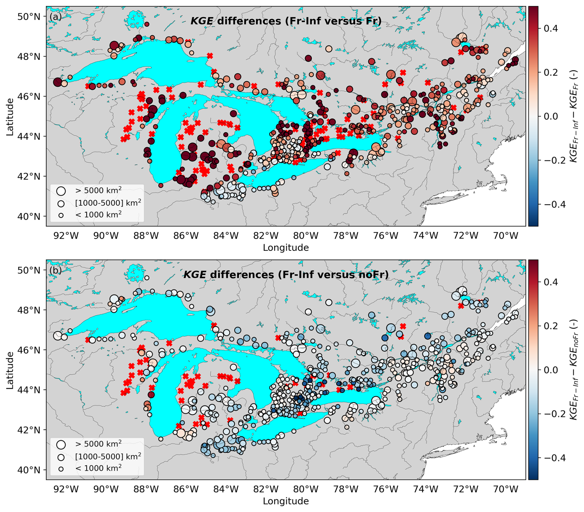
Figure 5 Same as Fig. 3 but for the differences between enhance frozen soil infiltration (Fr-Inf) and default soil freezing (Fr) experiments in (a) and between Fr-Inf and the experiment without soil freezing (noFr) in (b).

Compared to the noFr experiment, the Fr-Inf experiment generally degrades the KGE across the GLSL domain (degradation at 72 % of the stations; ΔKGE = −0.07). Unlike the Fr experiment, the Fr-Inf experiment results in fairly minor KGE degradations with a ΔKGE < –0.5 only at 4 stations (< 1 %). Consequently, more stations show improvements in KGE from the Fr-Inf experiment than from the Fr experiment, when compared to the noFr experiment. These improvements are concentrated in the southern part of Lake Ontario, the Saint-Lawrence River valley, and the vicinity of Lake Michigan. These regions encompass catchments with mixed surfaces of crops, grass, and forests (Fig. 2).

Figure 6 shows the boxplots of KGE, NSE and PBIAS for each of the three experiments. This comparison includes the 521 stations for which at least one experiment between the three resulted in an NSE greater than 0 or a KGE greater than −0.41. The noFr experiment produced the best results, while the Fr experiment produced the worst results in terms of KGE and NSE. While the Fr-Inf experiment does not outperform the noFr experiment, reducing ice impedance and removing saturation-excess runoff generation considerably improves the KGE and NSE metrics compared to the Fr experiment. These results align with those in Fig. 5.

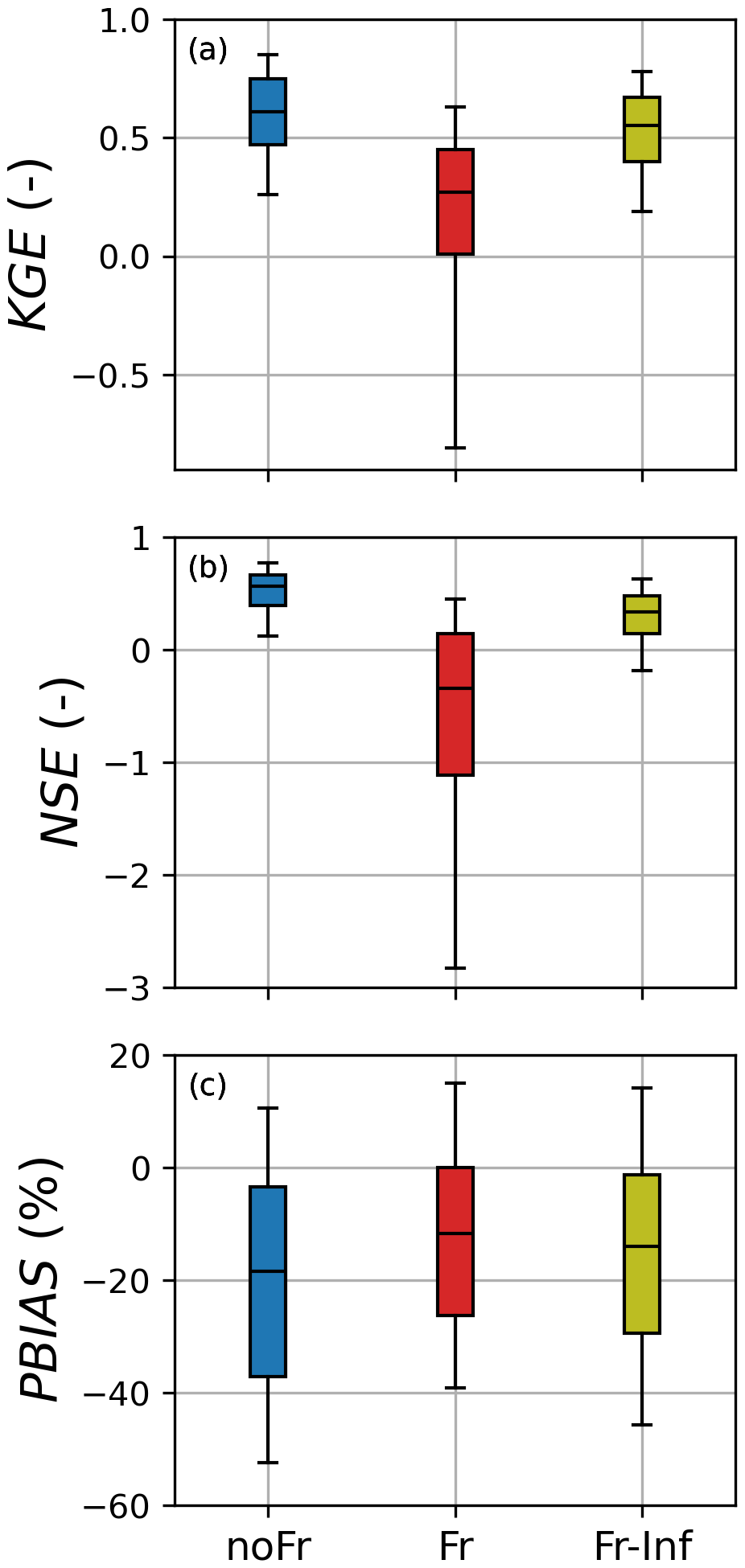
Figure 6 Boxplots of streamflow performances for the KGE in (a), the NSE in (b) and the PBIAS in (c) for the three configurations (noFr, Fr, Fr-Inf) in the Great-Lakes and Saint-Lawrence domain for the 2016–2021 evaluation period. Details on boxplot representation are given in the legend of Fig. 4. The target value for the KGE and NSE is 1.0 while the target value for the PBIAS is 0.0.

The noFr and the Fr experiments result in the largest and the smallest negative biases, respectively (Fig. 6c), contrasting with the KGE and NSE. This may be caused by the multiple unrealistically high mid-winter and spring peaks of streamflow which tend to compensate for SVS general tendency to underestimate baseflow. More interesting, however, is that the PBIAS of the Fr-Inf experiment is nearly equal to that of the Fr experiment. It suggests that the large improvements in KGE and NSE resulting from the addition of the enhanced frozen soil infiltration configuration do not exacerbate the general underestimation of streamflow.

Figure 7 illustrates the spatial distribution of KGE, NSE, and PBIAS for the Fr-Inf experiment, alongside the corresponding forest-crop and sand-clay fractions for each catchment. A distinct spatial pattern emerges across the GLSL domain with the Fr-Inf configuration reaching its highest scores for all three metrics in the Saint-Lawrence valley and north of Lake Superior and Lake Huron. These regions are characterized by a predominance of evergreen and mixed forests (Fig. 2) and sandy soils. Stations yielding KGE scores above 0.8 (yellow dots in Fig. 7a–c) are consistently associated with higher forest and sand fractions. Conversely, performance declines to approximately 0.4 in the regions between Lake Huron, Lake Ontario, and East of Lake Erie, which are areas dominated by crops and higher clay content. This aligns with the use of a fixed α_no-imp of 0.55 in Fr-Inf, which performs optimally in catchments with higher sand and forest fractions (Fig. S1). The lowest KGE (< 0) are obtained in the northern region between Lake Michigan and Lake Huron, and West of Lake Michigan, where the KGE is lower than 0 at many stations, regions with a high concentration of stations excluded from the experiment comparisons (red crosses on Figs. 3 and 5). One must note that the noFr and Fr experiments also exhibit better KGE in forested and sandy areas compared to agricultural and clayey regions (Figs. S2 and S3). This suggests that while activating soil freezing with enhanced infiltration modulates the KGE magnitude, it does not fundamentally drive the underlying spatial variability in model performance.

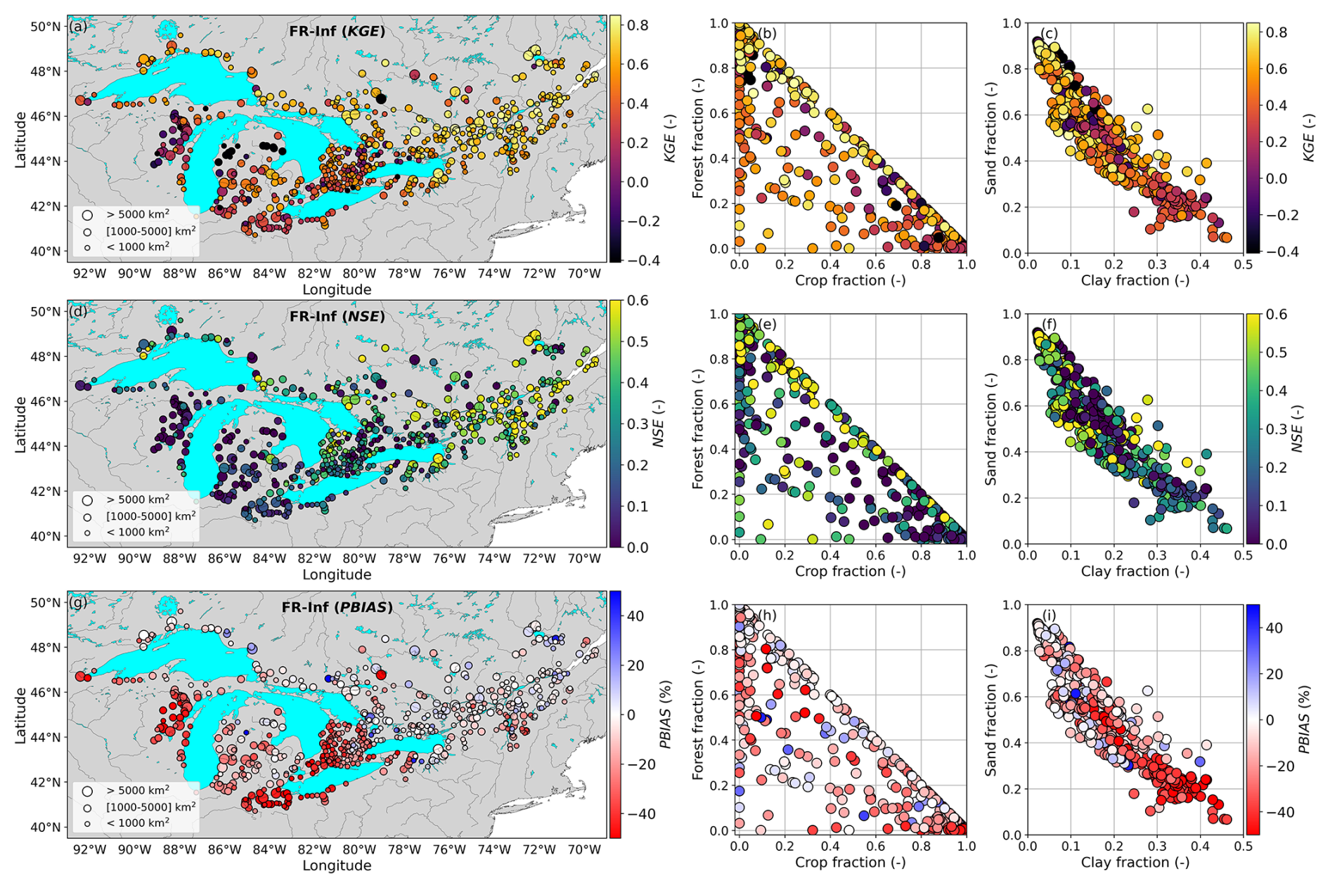
Figure 7 Spatial performance and catchment characteristics for the Fr-Inf experiment (2016–2021). Left panels (a), (d), (g) show the Great Lakes and Saint-Lawrence domain with KGE, NSE, and PBIAS at each station. Right panels (b), (c), (e), (f), (h), (i) show corresponding forest-crop and sand-clay fractions categorized by performance scores. In (a) to (f), a good performance of the model is represented by yellow shades. In (g) to (i), underestimation of streamflow is shown by red colors while an overestimation is shown by blue colors with pale red and blue dots show a low absolute bias.

The spatial pattern of the NSE closely follows that of the KGE, with the best results obtained in the northern and eastern parts of the GLSL domain (NSE > 0.5), and the worst scores obtained in the southern and western parts of the domain (NSE < 0.2). Accordingly, the NSE is better at stations associated with high forest and sand fractions. The similarity between the KGE and the NSE implies that the KGE can be explained by its variability component at most stations. Interestingly, the Fr experiment performs poorly (NSE < 0) across most of the domain, except for the region bounding Lake Erie (Fig. S3). Specifically, the Fr configuration yields higher NSE values in catchments characterized by clay-rich soils, a trend that contrasts with the results of the noFr and Fr-Inf experiments (Figs. S2 and 7). This suggests that the NSE, which reflects the ability of the model to capture the timing and amplitude of discharge peaks, is more sensitive to soil texture characteristics than the KGE.

In line with the KGE and NSE criteria, the absolute PBIAS is minimal (absolute values below 10 %; pale blue or red in Fig. 7c) for many stations located in the Saint-Lawrence Valley and North of Lake Superior and Lake Huron, where the soil tends to be sandy rather than clayey. In these regions, the Fr-Inf experiment slightly overestimates streamflow (blue dots) in general, though it tends to result in strong underestimations elsewhere. The positive bias is attributed to the soil freezing configuration that remains too restrictive to infiltration despite the increase of infiltration. Consequently, most stations in the eastern part of the domain, where the bias is positive, are also stations where the Fr-Inf degrades the KGE compared to noFr (Fig. 5b). The overall negative bias in the rest of the domain can be explained by an underestimation of streamflow during periods of low-flow regime. As the available pore space for liquid water decreases with growing soil ice, lateral flow likely prevails over soil drainage. This reduces the liquid water that contributes to support base flow. This behavior is consistent across all model configurations but is particularly pronounced in soils with higher clay fractions.

3.4 Impact of enhanced frozen soil infiltration on streamflow hydrographs and flux partitioning

Enhancing frozen soil infiltration in SVS results in changes in the behavior of simulated hydrographs. Figure 8 illustrates how the modeled streamflow varies between each experiment for three stations representative of different hydrological conditions within the GLSL domain. The Petawawa River flows eastward and drains a large forested area. The Saint-François River, that flows northward and drains an area almost twice as large as for the Petawawa River, is characterized by various surface types including crops, grassland and forests. The Thames River is located in Southern Ontario and drains a large agricultural catchment. In the Supplement, we also present hydrographs from three additional stations that drain large natural areas. The Richelieu River and the Ottawa River drain the two largest catchments in the GLSL domain, and the Mistassini River flows through a large boreal catchment. Mistassini River is also one of the northernmost stations in the domain.

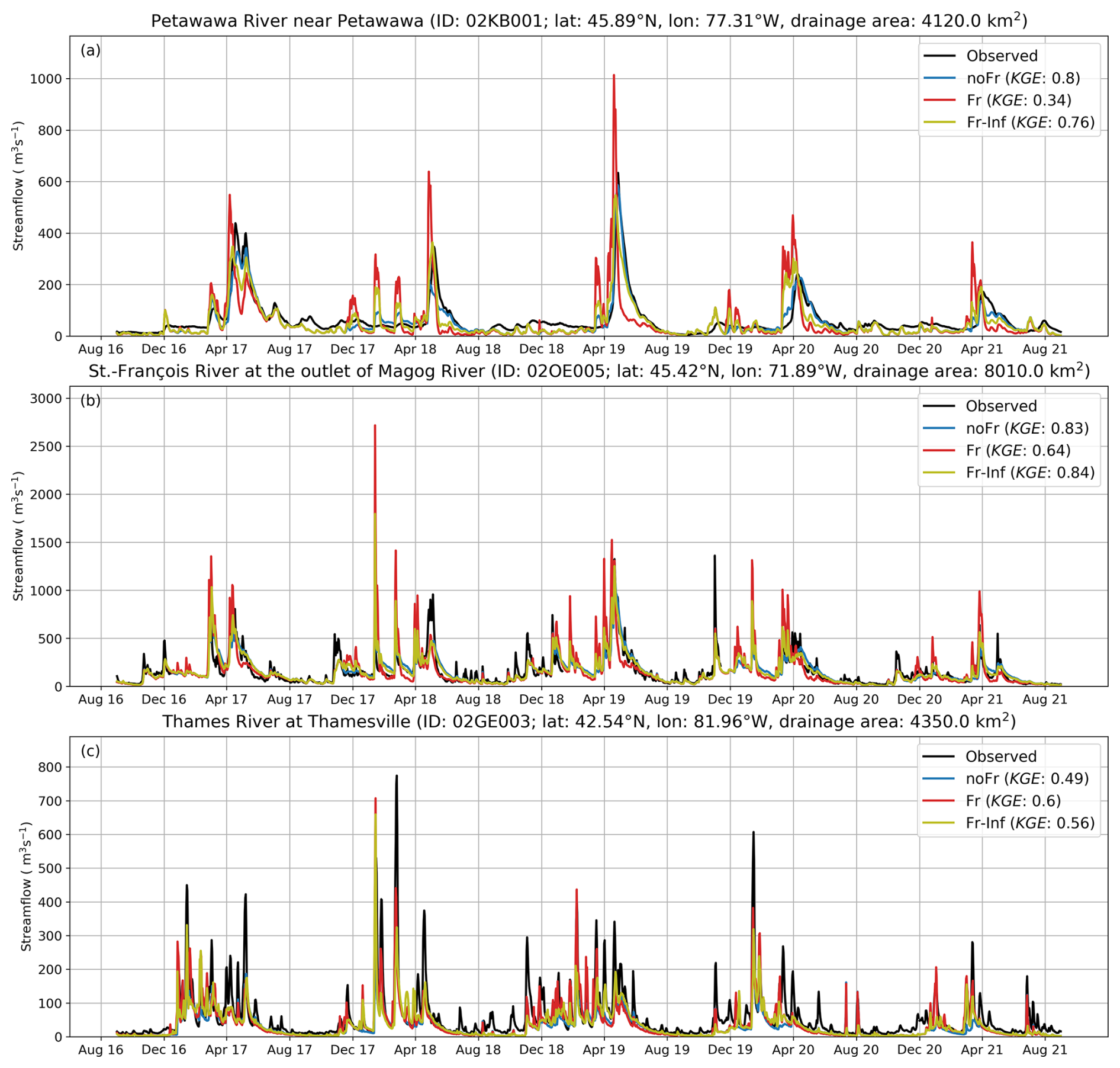
Figure 8 Observed and simulated streamflow of the Petawawa River (station ID: 02KB001) (a), the Saint-François River (station ID: 02OE005) (b) and the Thames River (station ID: 02GE003) (c) for the 2016–2021 evaluation period. Simulations of the no freezing experiment (noFr) are in blue, the soil freezing experiment (Fr) in red and the enhanced frozen soil infiltration (Fr-Inf) in yellow.

Across all catchments, enhancement of infiltration into the soil freezing scheme attenuates discharge peaks under frozen soil conditions while maintaining greater responsiveness than the experiment without soil freezing. For the Petawawa River (Fig. 8a), Fr-Inf produces a twofold increase in KGE relative to the Fr experiment, yet slightly underperforms compared to the noFr experiment (ΔKGE = −0.04). This minor discrepancy in KGE is attributed to erroneous simulations of mid-winter streamflow peaks and a steep recession limb in the spring hydrograph. In the case of the Saint-François River (Fig. 8b), where observed streamflow is slightly more responsive to mid-winter events, Fr-Inf substantially improves KGE compared to Fr, achieving a score of 0.84, slightly surpassing noFr. Conversely, for the Thames River (Fig. 8c), which features multiple winter peaks, enhanced infiltration leads to a slight degradation in KGE relative to Fr (ΔKGE = −0.04), though it remains a moderate improvement over noFr (ΔKGE = 0.07). In this specific catchment, the multiplicative factors of m_h = 500 and m_v = 10 may be insufficient to adequately represent the effects of agricultural drainage, highlighting a limitation of this non-explicit approach (Gaborit et al., 2025). The hydrographs from the three catchments presented in Fig. S4 show similar results. Fr-inf clearly improves the performance compared to Fr and results in similar or slightly degraded performance compared to noFr. It demonstrates that fostering infiltration into the soil freezing scheme of SVS improves streamflow simulations for catchments of various landscapes and sizes. On both Figs. 8 and S4, differences between the assessed SVS configuration under unfrozen soil conditions arise due to the structural modification to surface runoff generation. These differences remain uncommon since it necessitates the saturation of the surface layer, which rarely occurs without modelled soil ice.

Figure 9 shows an example of how each surface hydrological flux is simulated under each of the three model configurations. In this example, we present the case of the Moira River at the station near Foxboro (NSRPS station ID: 02HL001). The Moira River flows through a natural, mostly forested catchment located north of Lake Ontario. During the period from 2016 to 2021, the peak flow varied between 100 m³ s⁻¹ (in 2021) and 275 m³ s⁻¹ (in 2017), while the low flow approached 0 m³ s⁻¹ every summer (Fig. 9a). All three model configurations have the tendency of simulating peaks of discharge in winter that are not observed at the gauging station. This could be explained by the presence of numerous wetlands and meanders in the area, which have the effect of attenuating runoff peaks during rain and thaw events. These processes are not yet fully represented in Watroute.

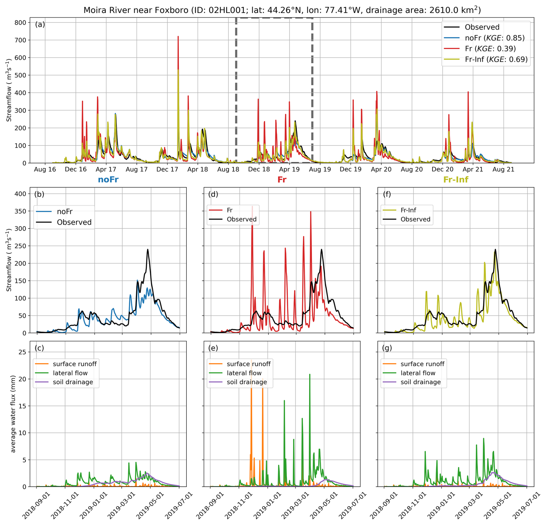
Figure 9 Observed and simulated streamflow at the Moira River (station ID: 02HL001) for the 2016–2021 evaluation period with the specific year 2018–2019 identified with the dashed line (a). The streamflow simulated with the noFr, Fr and Fr-Inf configurations for the 2018–2019 year is shown against the observed streamflow in (b), (d) and (f), respectively. Water fluxes from SVS (surface runoff, lateral flow and soil drainage) averaged over the drainage area of station 02HL001 for the year 2018–2019 period are presented for each experiment on (c), (e) and (g).

A detailed examination of the September 2018 to June 2019 period reveals distinct differences in streamflow simulations at station 02HL001 across the model configurations. Relative to the Fr and Fr-Inf experiments, the noFr configuration produces the highest winter base flow, yet exhibits the most significant underestimation of spring peak flow (Fig. 9b). The large base flow is attributed to persistent soil drainage, driven by continuous infiltration and percolation (Fig. 9c, purple curve). As a result, the reduced surface runoff and lateral flow in spring (orange and green curves) constrain the magnitude of spring freshets for this experiment and this station.

In contrast, the Fr experiment displays markedly different hydrograph dynamics, featuring frequent high-magnitude discharge events in winter and spring alongside low base flow (Fig. 9d). This behavior is attributed to early-winter surface runoff peaks (Fig. 9e, orange curve) followed by lateral flow peaks from January onward (green curve). Soil ice accumulation in near-surface layers during early winter reduces effective porosity, thereby enhancing saturation-excess runoff generation (Alavi et al., 2016). Subsequently, as the freezing front advances deeper into the soil column, increased saturation in subsurface layers forces excess water to discharge as lateral flow. As a result, percolation to the deep soil layers is negligible, effectively limiting the drainage contribution to base flow (Fig. 9e, purple curve).

The enhanced frozen soil infiltration configuration represents an effective compromise between the noFr and Fr configurations. Specifically, Fr-Inf attenuates winter peaks in favor of base flow and yields a more accurate simulation of the spring freshet compared to Fr (Fig. 9f). Mitigating runoff caused by surface layer saturation reduces the surface runoff component (Fig.  9g, orange curve) and facilitates water redistribution into lower soil layers. Furthermore, percolation is promoted when the no-impedance criterion (α_no-imp > 0.55) is satisfied. This results in dampened lateral flow peaks during winter and spring, coupled with an increased contribution of soil drainage to the spring peak flow (Fig. 9g, green and purple curves). Yet the Fr-Inf experiment still leads to hydrologic behavior that is too flashy for this station, but as explained earlier, this could be due to the fact that the effects of the meanders and wetlands along this river are not currently well captured by the Watroute model used here. One must also note that the impact of the Fr-Inf configuration on streamflow simulations varies among stations and years depending on the prevailing soil freezing conditions which differ spatially and inter-annually.

3.5 Evaluation of near-surface meteorology and depth of frozen soil

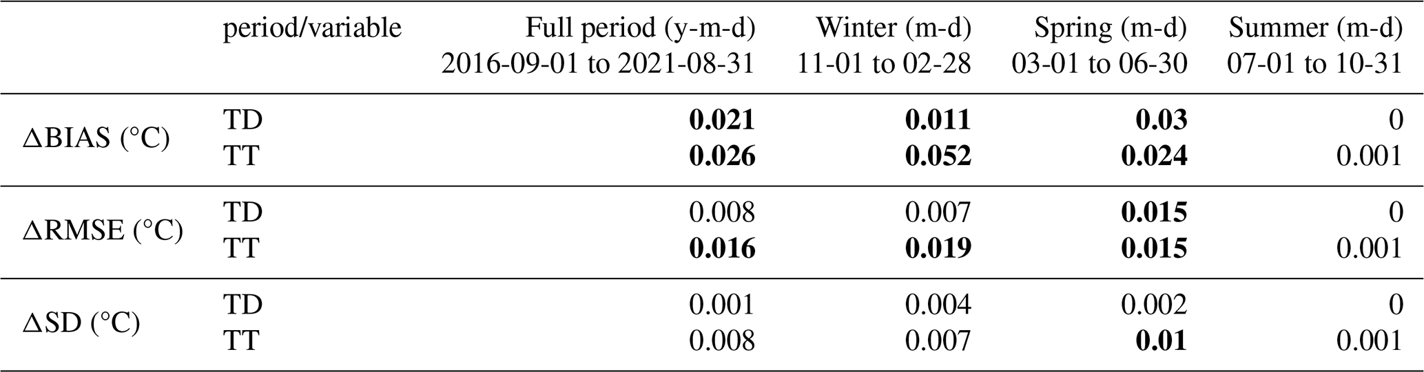
Given the upcoming implementation of the soil freezing scheme of SVS within the operational framework of ECCC for numerical weather predictions, it is critical to evaluate how the proposed configuration affects surface variables. Table 1 details the changes in performance metrics (ΔBIAS, ΔRMSE and ΔSD) between the Fr-Inf and noFr experiments for near-surface dewpoint (TD) and air (TT) temperatures, analyzed both over the full period and seasonally. The enhanced frozen soil infiltration configuration results in either neutral performance or slight improvements across all metrics. In general, improvements are statistically significant during nighttime (not shown). Notably, improvements are greater for TT than for TD, and are more important in winter compared to spring, while remaining neutral in summer. Similar results comparing Fr and noFr (Table S1 in the Supplement) suggest that these benefits stem primarily from the activation of the soil freezing module rather than the enhancement of infiltration. Consequently, the new configuration does not compromise the quality of surface variable estimation. Rather, it provides slight improvements under conditions favorable to soil freezing.

Table 1 Differences of the bias (BIAS), root mean square error (RMSE) and standard deviation of the error (SD) for the 2 m dew point temperature (TD) and the 2 m air temperature (TT) between the enhanced frozen soil infiltration experiment (Fr-Inf) and the experiment without soil freezing (noFr). The performances are evaluated over the full period (from 1 September 2016 to 31 August 2021) and seasonally with winter period spanning from 1 November to 28 February, spring period from 1 March to 30 June and summer period from 1 July to 31 October. Positive values greater than 0.01 °C are shown in bold and represent an improvement of the Fr-Inf experiment compared to noFr.

The integration of soil freezing into SVS is particularly valuable, as it yields additional output variables of potential interest for external users. It is therefore imperative to assess the accuracy of soil freezing simulations relative to observational data. Figure 10a compares the observed freezing depth, averaged across 103 stations in the central US, with results from the Fr and Fr-Inf experiments. Both configurations show strong agreement with observations regarding amplitude and interannual variability. The freezing depth simulated by Fr-Inf is slightly reduced compared to Fr. This is likely explained by higher water retention in deep soil layers in the Fr-Inf configuration, resulting from enhanced infiltration. Consequently, the increased soil moisture imposes a higher energy requirement to freeze the liquid water content of a given layer.

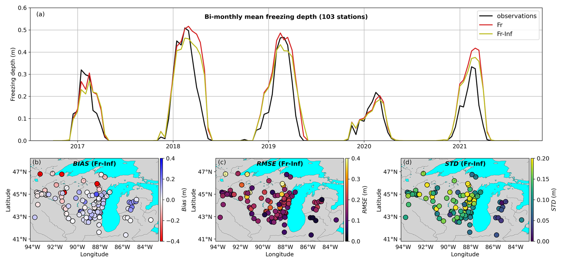
Figure 10 Bi-monthly mean of freezing depth for 103 stations located in the central US from 2016 to 2021 with observations shown in black and soil freezing (Fr) and enhanced frozen soil infiltration (Fr-Inf) simulations shown in red and yellow, respectively (a). The BIAS, RMSE and standard deviation (SD) at each station over the 2016–2021 period for the Fr-Inf experiment are respectively shown in (b), (c) and (d).

Figures 10b–d illustrate the spatial distribution of the 103 stations across the central US, with the BIAS, RMSE, and SD of the Fr-Inf experiment represented by color gradients. At most stations, Fr-Inf overestimates freezing depth (blue dots in Fig. 10b), except for a distinct cluster in the northern region. These stations correspond to the highest RMSE values, though not necessarily to the highest SD, implying a consistent underestimation of freezing depth throughout winter and spring. In general, stations where Fr-Inf overestimates freezing depth coincide with low RMSE values (< 0.15 m), which indicate that Fr-Inf is a reliable predictor of freezing depth. However, locations with higher SD values exhibit a greater deviation between the model and the observations and consequently a large temporal variability. A similar spatial pattern is observed for the Fr experiment (see Fig. S5).

4 Discussion

In the current study, we present an updated soil freezing scheme for the SVS land surface model that includes two major structural changes: the removal of the ice-impedance effect on the vertical soil water fluxes above a calibrated soil moisture threshold and the use of infiltration capacity as the only driver for surface runoff generation. Here, we compare our performance against similar large-scale land surface modeling studies and outline the limitations of both our approach and the experimental modeling setup.

4.1 Comparison with other studies

Koren et al. (2014) assessed the impact of a physically-based modified version of the Sacramento Soil Moisture Accounting model (SAC-SMA) to account for the effect of frozen soil on runoff dynamics in 11 large US Midwest catchments. In this approach, the effect of ice on the increase in the soil particle-water contact surface is considered in the calculation of a reduced K_sat,v, which is later used in the SAC-SMA model to estimate runoff generation under frozen soil conditions. This modification resulted in an improved representation of winter and spring hydrograph peaks compared to non-frozen conditions, which contrasts with our findings where the noFr experiment outperformed Fr over the GLSL domain. This divergence is likely attributable to the use of an empirical ice-impedance factor in SVS to impede soil water flow, which is more restrictive to infiltration than the parameterization from Koren et al. (2014). The ice-impedance configuration used in SVS is the same as the one used in the CLASS land surface model (Ganji et al., 2017), which is based on a silty clay loam site in Saskatchewan and derived from Zhao and Gray (1997). The limitations of using such impedance factors to restrict frozen ground infiltration are well documented by Kurylyk and Watanabe (2013).

Ganji et al. (2017) performed a streamflow evaluation of the Canadian Land Surface Scheme (CLASS; Verseghy, 2008) coupled with Watroute (Kouwen, 2010) across 12 catchments in Québec's boreal, subarctic, and arctic regions. They reported improved agreement with observations when the impedance factor (same as in SVS) was tuned to be more restrictive but with a dual-domain infiltration configuration (Niu and Yang, 2006). In another study, Agnihotri et al. (2023) tested various frozen soil hydraulic property schemes within Noah-MP in the Mississippi River basin, finding that streamflow simulations were also improved using the Niu and Yang (2006) configuration but without any ice-impedance factor. Both Ganji et al. (2017) and Agnihotri et al. (2023) obtained optimal results using configurations that facilitate infiltration into frozen ground. This aligns with our finding that activating the enhanced frozen soil infiltration configuration in SVS improves streamflow simulations. Since these studies and ours cover diverse geographical domains, it suggests that permitting infiltration into frozen soil is critical for accurate large-scale hydrological modeling. A configuration of SVS using the dual-permeability approach from Agnihotri et al. (2023) was also evaluated. This simple configuration resulted in a marked degradation in model performance compared to the Fr-Inf configuration (Fig.  S6). These results demonstrate that while Fr-Inf does not explicitly account for the spatial heterogeneity of subgrid macropore networks, it remains a suitable and effective approach for enhancing frozen ground infiltration and improving streamflow simulations at the catchment scale. Notably, we achieved performance metrics comparable to Agnihotri et al. (2023) with a median KGE of 0.55 without a dual-domain approach. Although the studies from Ganji et al. (2017), Agnihotri et al. (2023) and ours cover different cold geographical domains, it has been suggested that in permafrost-dominated regions, infiltration should be restricted in LSS to better simulate streamflow (Swenson et al., 2012).

4.2 Limitations

While some studies have shown that preferential flow is favored under low antecedent soil moisture (Hardie et al., 2011; Merdun et al., 2008), the approach proposed here relies on the exceedance of a soil water content threshold, derived from sensitivity analysis, to increase frozen soil infiltration. Empirical studies have suggested that water may freeze first in small pores, leaving connected, air-filled larger pores available for rapid infiltration (Demand et al., 2019; Mohammed et al., 2019; Bauer et al., 2026). This is favored by a large soil pore-size distribution at small scale driven by biological factors, such as earthworm burrows and root channels (Jarvis, 2007; Six et al., 2004), and by pore-structure effects associated with high textural heterogeneity (Beven and Germann, 2013). Nevertheless, the approach introduced here remains a structural modification to the SVS soil freezing scheme which does not explicitly account for these subgrid physical processes that drive frozen ground infiltration. Moreover, the proposed parameterization does not currently rely on land cover characteristics neither on soil texture to modulate infiltration, despite well-documented effects on frozen soil hydraulic behavior (Ala-Aho et al., 2021; Jarvis, 2007; Mohammed et al., 2019; Zhang et al., 2021). Our results further suggest that the observed spatial variability in model performance is influenced by land use and, to a larger extent, by soil texture (Fig. 7). Better performance achieved in forested and sandy catchments is attributed to the calibration of the α_no-imp parameter to 0.55, which is more representative of these specific landscape characteristics. However, to maintain model parsimony and avoid introducing additional free parameters, the current Fr-Inf configuration does not explicitly account for varying surface characteristics. Despite this simplification, the approach performs reasonably well across the Great Lakes and Saint-Lawrence domain. In the future, the calibration of α_no-imp is likely to be reviewed when applying the model across other large domains in Canada and this approach may be revised to include a root-depth or a soil-texture dependency.

Additionally, SVS does not include a representation of soil organic matter despite known relationships between peat composition and degradation, pore structure and hydraulic properties of the vadose zone (Decharme, 2025; Liu and Lennartz, 2019). Indeed, governing pedotransfer equations in SVS neglects effects of soil structure, land cover and climate, among other factors. Finally, given the reliance of the SVS vertical flux scheme on Darcian flow (Alavi et al., 2016), we tried to mimic preferential flow to increase vertical hydraulic conductivity (K_sat,v) but this resulted in numerical instabilities. Overall, a comprehensive reformulation of the soil water transfer module is necessary to include preferential flow in SVS and represent more accurately downward gravitational flow that occurs in macropores under frozen soil conditions (Mohammed et al., 2019), and more broadly to improve the robustness and transferability of the model.

Certain limitations are inherent to the SVS soil freezing scheme. While modifications were introduced to the soil thermal regime formulation of Amani et al. (2025) to better represent freezing depth, the existing SVS soil freezing module retains significant simplifications. These include the use of the Hayashi et al. (2007) heat conduction algorithm and the neglect of freezing point depression. Furthermore, SVS employs a single-layer snowpack representation whose thermal regime is based on a force-restore scheme (Leonardini et al., 2021). These simplifications constrain the simulation of soil temperature evolution and the associated soil water phase changes. Recently, SVS version 2.0 (SVS2) was released (Vionnet et al., 2025), featuring completely reformulated schemes for soil freezing and snowpack evolution. Note that efforts are currently ongoing to include organic soil into SVS2. Comparative research is underway to evaluate both SVS versions focusing on frozen ground infiltration.

Streamflow simulations under frozen soil conditions are governed by the parameterization of soil water fluxes in SVS. Surface runoff and lateral flow are partially generated via a subgrid-scale interflow parameterization (Soulis et al., 2011). This mechanism was initially parametrized in SVS to represent subsurface flow but also applies to the surface soil layer by configuration. Its impact on surface runoff under unfrozen soil conditions is negligible but was found to be major in the presence of soil ice in the topmost soil layer. To isolate the effects of each modification, we conducted two intermediate frozen soil sensitivity experiments (Fig. S7). Disabling the subgrid-scale surface runoff generation as the sole modification resulted in only slight improvements over the default soil freezing configuration (Fr). Similarly, applying the Fr-Inf configuration while restoring the surface runoff generation mechanism yielded only minor performance gains compared to Fr. These tests demonstrate that both modifications are necessary to meaningfully improve model performance under frozen soil conditions and should therefore be implemented together in SVS. However, while these combined changes successfully reduce rapid-response fluxes, the Fr-Inf configuration still overestimates mid-winter runoff peaks (Figs. 8 and 9). This can be partly explained by the near-surface anisotropy ratio ($K_{\mathrm{sat},\mathrm{h}}/K_{\mathrm{sat},\mathrm{v}}$), which is of the order of 1000 and strongly promotes lateral flow over infiltration. Current efforts focus on refining the lateral flow formulation in SVS by incorporating new anisotropy estimations based on Brooks et al. (2004) and Decharme et al. (2013).

Finally, the Watroute routing model lacks groundwater reservoir exchanges and has known limitations in simulating flow within meandering regions and wetland areas (Gaborit et al., 2025). By design, Watroute cannot explicitly represent lateral spreading of water in flat areas adjacent to the river, as the model assumes a uniform overbank slope of 1 %. This likely contributes to the poor performance observed in the region bounded by the five Great Lakes (Fig. 7) and the exclusion of several stations for analysis in this region (Figs. 3 and 5). The envisioned transition in NSRPS from Watroute to the Raven routing scheme, which includes an explicit representation of wetlands (Craig et al., 2020), in the coming years may help alleviate these issues.

5 Conclusion

In this work, we proposed a new configuration of soil freezing within SVS, the land surface component of the GEM-Hydro hydrometeorological modelling platform, to increase infiltration. The evaluation, performed against observations from over 580 hydrometric stations in the Great-Lakes and Saint-Lawrence domain over five years, indicates that enhancing infiltration under frozen soil conditions yields improved streamflow performances at 88 % of the stations for which a comparison was performed with the median KGE increasing by 0.28, without outperforming a configuration without soil freezing overall. The improved configuration utilizes unimpeded hydraulic conductivity when liquid water content surpasses a specific threshold relative to available pore space and prevent surface runoff generated from subgrid-scale saturation interflow. This configuration promotes soil drainage at the expense of surface runoff and lateral flow, thereby improving the simulation of winter flow and spring freshet. The new enhanced frozen soil infiltration scheme further provides an accurate freezing depth estimation without compromising performance for near-surface variables (dew point and air temperature).

Our findings demonstrate that the updated soil freezing scheme is capable of accurately estimating streamflow across large hydrological domains. Future work will focus on evaluating this improved SVS version within GEM-Hydro across Canada. This assessment is a prerequisite for the operational implementation of the soil freezing formulation in the NSRPS. Ultimately, improving the representation of soil freezing and thawing in SVS is a critical step toward its adoption as the operational land surface scheme within the GEM-based numerical weather prediction systems of ECCC.