Limits to GRACE-based groundwater storage monitoring in a 23 000 km² coastal basin: evidence from the Lower Kutai Basin, Indonesia

Groundwater is considered a climate-resilient source of freshwater yet its long-term response to climate variability remains poorly understood in environments with limited ground-based monitoring networks. In the Lower Kutai Basin where Indonesia's new capital (Nusantara) is under development, we examine the limitations to Gravity Recovery and Climate Experiment (GRACE) satellite data to estimate groundwater storage changes (ΔGWS) over the last two decades using evidence of other water storage changes from global-scale models. We identify potential ocean signal leakage, inferred from residual correlations (r up to 0.68) between paired land-ocean grids, which can propagate errors into ΔGWS estimates and result in physically implausible ΔGWS values. GRACE-derived terrestrial water storage anomalies (ΔTWS) exhibit strong seasonal and interannual variability that is consistent across different spatial scales ($r=\mathrm{0.78}-\mathrm{1}$) and are dominated by changes in root-zone soil moisture storage (ΔSMS). Across 54 realizations, only 21 %–60 % (mean: 42 %) of ΔGWS estimates per realization are physically plausible. Validation of plausible ΔGWS values critically relies on robust storage coefficients. Correlations between GRACE-derived ΔGWS and groundwater-level anomalies (ΔGWL) are generally weak and reflect discrepancies between GRACE's basin-scale signals and localized aquifer dynamics influenced by heterogeneity and groundwater abstraction. Statistical analyses show weak-to-moderate coupling of ΔTWS and ΔSMS with ENSO indices ($r=-\mathrm{0.4}$ to −0.6) whereas ΔGWS is less responsive. Drought conditions associated with the 2015–2016 El Niño are a notable exception as ΔTWS deficits (−2.4 to $-\mathrm{4.6}\mathrm{cm}{\mathrm{month}}^{-\mathrm{1}}$) correspond with plausible ΔGWS declines ($-\mathrm{1.1}\mathrm{cm}{\mathrm{month}}^{-\mathrm{1}}$). High-frequency (hourly) groundwater-level observations indicate that episodic, high-intensity rainfall events (>90th percentile) disproportionately contribute to groundwater recharge. These findings demonstrate that only a subset of ΔGWS values can be plausibly estimated from GRACE so that, without expanded in situ monitoring, ΔGWS estimates in this small coastal basin will remain highly uncertain.

1 Introduction

Reliable freshwater resources are essential for sustaining human life, supporting aquatic ecosystems, agricultural productivity, and economic stability (Kundzewicz, 2007; Koehler, 2008; Pimentel et al., 1997; Chakravorty and Zilberman, 2000; Pradinaud et al., 2019; Wilson and Carpenter, 1999). Groundwater serves as a crucial climate-resilient water source (Cuthbert et al., 2019a; Taylor et al., 2013b), storing ∼24 million km³ of global water reserves to a depth of 2 km (Gleeson et al., 2016; Ferguson et al., 2021). It supplies about one-third of the world's agricultural irrigation and drinking water needs (Müller Schmied et al., 2021). Excessive groundwater abstraction has, however, led to global-scale groundwater depletion (Jasechko et al., 2024; Wada et al., 2010; Konikow and Kendy, 2005; Bierkens and Wada, 2019).

Understanding groundwater storage responses to climate variability and change helps to inform the resilience of groundwater withdrawals to meet increasing freshwater demands (Taylor et al., 2013b; Cuthbert et al., 2019a; Loaiciga and Doh, 2024; Wada et al., 2011; Ferguson and Gleeson, 2012). Such understanding is constrained in the Lower Kutai Basin (LKB) of Indonesia where the country's new capital (Nusantara) is under development, by limited, ground-based monitoring. Freshwater demand in Nusantara is projected to increase at least fourfold for domestic use alone by 2045 (Susantono, 2022). Seasonal imbalances between supply and demand along with potential construction delays can lead to intensified groundwater abstraction for domestic, industrial, and agricultural water use through the drilling of private wells (Grönwall and Danert, 2020). Assessing historical groundwater storage (GWS) changes in response to pumping and recharge is required to inform renewable groundwater use within the basin (Cuthbert et al., 2023).

Recent advancements in satellite-based remote sensing have enabled the monitoring of terrestrial water storage (TWS) changes using Gravity Recovery and Climate Experiment (GRACE) datasets across diverse hydrological settings at both global (Ndehedehe et al., 2023; Shamsudduha and Taylor, 2020; Thomas et al., 2017; Li et al., 2019; Jin and Feng, 2013; Forootan et al., 2024; Rodell et al., 2024) and basin scales (Rodell et al., 2009; Asoka et al., 2017; Zhang et al., 2024; Rateb et al., 2020; Thomas and Famiglietti, 2019; Ouma et al., 2015). GRACE detects mass variations by measuring changes in Earth's gravity field, which, once corrected for atmospheric and oceanic effects, primarily reflect changes in terrestrial water storage (ΔTWS) (Landerer and Swenson, 2012). ΔTWS encompasses changes in soil moisture, surface water, snow, groundwater, and vegetation water content (canopy storage). Accounting for changes in soil moisture, surface water, snow and canopy storage using global-scale (e.g. Global Land Data Assimilation System, GLDAS) simulations, GRACE enables the indirect estimation of changes in groundwater storage (ΔGWS) as a residual component (Zhang et al., 2024; Shamsudduha and Taylor, 2020; Thomas et al., 2017; Ouma et al., 2015; Rodell et al., 2009; Arifin et al., 2025b).

Climate variability is widely recognized as a key driver of ΔTWS variability (Scanlon et al., 2022, 2023; Rodell et al., 2024; Bolaños et al., 2021; Thomas and Famiglietti, 2019; Ni et al., 2018). Among the most pervasive large-scale controls on climate variability is the El Niño–Southern Oscillation (ENSO), a coupled ocean–atmosphere phenomenon originating in the equatorial Pacific Ocean (Trenberth, 1997). ENSO influences precipitation patterns, evapotranspiration rates, and atmospheric circulation (Gu and Adler, 2019; Xu et al., 2004; Tamaddun et al., 2019; Sabziparvar et al., 2011; Moura et al., 2019; Ruiz-Vásquez et al., 2024), thereby modulating water storage dynamics. ENSO events are broadly classified into El Niño (warm phase) and La Niña (cool phase), each of which alters hydrological conditions worldwide. El Niño events typically induce drier-than-normal conditions in regions such as Australia, southern Africa, central China, and Southeast Asia while increasing rainfall in parts of South America, southern China, and East Africa (Wang et al., 2014; Generoso et al., 2020; Kovats, 2000). Conversely, La Niña episodes generally produce the opposite effects in these regions.

Large-scale climatic teleconnections can manifest as fluctuations in ΔTWS and ΔGWS. Studies investigating the relationship between climate indices and ΔTWS anomalies using GRACE data have reported moderate to high correlations (Ni et al., 2018; Phillips et al., 2012; Scanlon et al., 2022; Bolaños et al., 2021; Anyah et al., 2018; Pereira et al., 2024). For instance, strong regional correlations between GRACE ΔTWS and ENSO have been observed in West and East Africa, Venezuela/Colombia, and Borneo (Phillips et al., 2012; Anyah et al., 2018). Additionally, several studies have demonstrated a relationship between GRACE-derived ΔGWS and ENSO events (Vissa et al., 2019; Kolusu et al., 2019; Forootan et al., 2024; Song et al., 2024), highlighting the role of ENSO in driving interannual groundwater storage variability.

The applicability of GRACE data to assess climate-related ΔTWS and ΔGWS anomalies at spatial scales smaller than the native GRACE resolution of ≥90 000 km² (Loomis et al., 2021; Tapley et al., 2004; Shamsudduha and Taylor, 2020; Wiese et al., 2016) remains poorly characterized. Although Level-3 GRACE datasets are publicly available at higher spatial resolutions such as GRACE CSR at 0.25° and GRACE GSFC at 0.5°, these are resampled from the original coarse-resolution data (Save et al., 2016). Consequently, individual grids are spatially correlated and do not contain independent ΔTWS signals at scales smaller than GRACE's native resolution (Vishwakarma et al., 2021). Various downscaling techniques have been increasingly applied to estimate ΔTWS and GRACE-derived ΔGWS at finer spatial resolutions. These approaches range from statistical modelling to data-assimilation frameworks incorporating machine-learning algorithms (Vishwakarma et al., 2021; Miro and Famiglietti, 2018; Zhong et al., 2021; Fatolazadeh et al., 2022; Yin et al., 2018; Kalu et al., 2024; Verma and Katpatal, 2020; Yin et al., 2022; Yazdian et al., 2023). Although these methods offer practical insights in estimating GRACE-derived ΔGWS, most remain insufficiently validated. The lack of ground-based observations introduces substantial uncertainty in evaluating the reliability of downscaled GRACE products, particularly for assessing groundwater dynamics at sub-basin scales. Moreover, GRACE ΔTWS estimates are susceptible to signal leakage due to filtering processes, a challenge particularly pronounced in small catchments (Vishwakarma et al., 2016; Vishwakarma et al., 2018). Hydrological models are often used to reduce leakage effects (Landerer and Swenson, 2012; Wiese et al., 2016; Longuevergne et al., 2010); however, model-based corrections can propagate errors and uncertainties (Vishwakarma et al., 2016).

This study examines what groundwater storage changes GRACE can and cannot resolve in a small (23 000 km²), coastal and data-scarce basin of Indonesia (Lower Kutai Basin), where spatial scale and proximity to the ocean increase the risk of signal leakage and attenuation. Specifically, we (1) compare ΔTWS across multiple GRACE products, (2) evaluate the potential for ocean leakage into inland GRACE grids, (3) assess the plausibility of GRACE-derived ΔGWS against limited piezometric data, and (4) examine whether large-scale climate drivers, particularly ENSO, are detectable. The aim is to evaluate the limits of GRACE in this challenging setting and to demonstrate that without a substantially expanded piezometric network, neither GRACE nor in situ observations alone can provide robust groundwater storage estimates.

2 Materials and methods

2.1 Study area

The study area is located within the Lower Kutai Basin (LKB) in East Kalimantan, Indonesia (Fig. 1). It is covered by eight 0.5° grids, which can be further subdivided into smaller 0.25° grids. This region spans approximately 23 000 km² and encompasses diverse landscapes including coastal lowlands, the Mahakam Delta, and hilly uplands with elevations ranging from below 50 m above sea level (m a.s.l.) to 750 m a.s.l. Most of the area is covered by forest (Zanaga et al., 2022). Lakes are concentrated in the northwest of the study area, with a few surrounding wetlands and peatlands (Patria et al., 2025; Omar et al., 2022) and represented by their maximum surface water extent (Pekel et al., 2016) shown in Fig. 1.

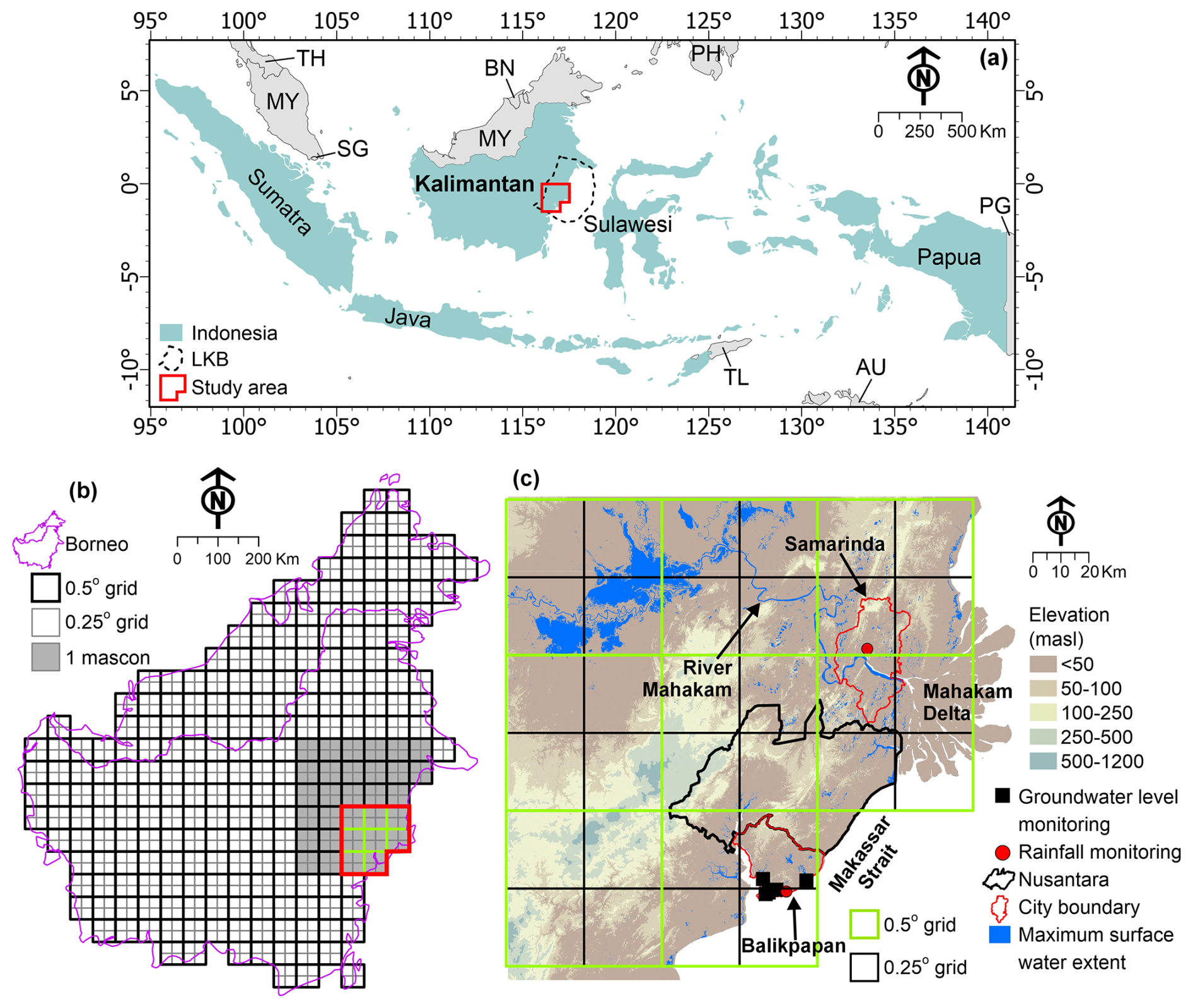
Figure 1 (a) Study area within the Lower Kutai Basin (LKB) of East Kalimantan, Indonesia. (b) Distribution of 0.5° and 0.25° grids over Borneo. (c) Elevation data (BIG, 2022), maximum surface water extent (Pekel et al., 2016), and grid distribution across the study area. Green 0.5° grids indicate the selected grids for the study area. Country boundaries are from ESRI (2022) and country abbreviations (e.g., TH, SG, MY) follow ISO codes. © Badan Informasi Geospasial (BIG), 2022. All rights reserved. Global Surface Water dataset ©European Commission, Joint Research Centre (JRC). Esri 2022 | Powered by Esri.

The LKB is primarily drained by the River Mahakam, the largest river system in East Kalimantan which flows eastward into the Makassar Strait, forming an extensive deltaic system. The river provides ∼70 % of the freshwater supply for Samarinda (BPS-Statistics of Kalimantan Timur Province, 2022), the capital city of East Kalimantan Province, whereas the remaining 30 % comes from groundwater. In Balikpapan City located south of Nusantara, groundwater serves as the primary water source supplying ∼70 % of the total water demand (Irsyadulhaq et al., 2024).

Arifin et al. (2024) provide surface geological and hydrogeological maps of the coastal LKB. The regional hydrostratigraphy is primarily composed of Miocene to Quaternary deltaic deposits which are extensively distributed across the coastal LKB (KESDM, 2022; Moss and Chambers, 1999). These deposits mainly consist of interbedded sand and clay layers, forming a complex aquifer system that may extend offshore toward the Makassar Strait (Arifin et al., 2025a). The primary aquifers are sand-dominated sequences that exhibit significant variability in hydrogeological properties, ranging from low-productivity zones with substantial clay content to highly productive horizons where coarse-grained sands are prevalent (KESDM, 2022).

2.2 GRACE data

Monthly terrestrial water storage anomalies (ΔTWS) data from 2002–2023 were obtained from five Level-3 GRACE datasets: the GRACE Jet Propulsion Laboratory (JPL) RL06.3Mv04 (Landerer et al., 2020; Watkins et al., 2015; Wiese et al., 2023; Wiese et al., 2016) sourced from the NASA PO.DAAC portal (https://podaac.jpl.nasa.gov/, last access: 18 October 2024); the GRACE CSR RL06.3 (Save et al., 2016; Save, 2020) available from the Center for Space Research (CSR) at the University of Texas at Austin portal (https://www2.csr.utexas.edu/grace/, last access: 18 October 2024); the GRACE GSFC RL06v2.0 (Loomis et al., 2019) provided by the NASA Goddard Space Flight Center (GSFC) via the NASA GSFC portal (https://earth.gsfc.nasa.gov/geo/data/grace-mascons, last access: 18 October 2024); GRACE GFZ RL06 and GRACE Combination Service for Time-variable Gravity Fields (COST-G) RL01 provided by German Research Centre for Geosciences (GFZ) Data Services via https://gravis.gfz.de/tws (last access: 12 August 2025) (Boergens et al., 2020, 2019, 2022; Dahle et al., 2025); these datasets are derived from GRACE and its successor, GRACE Follow-On (FO). The recently released JPL, CSR, and GSFC products employ mascons whereas GFZ and COST-G are based on spherical harmonic solutions.

The downscaled GRACE JPL and GRACE GSFC datasets provide submascon fields on a 0.5° grid, whereas the downscaled GRACE CSR dataset offers a finer 0.25° grid resolution. Both GRACE GFZ and COST-G products have a 1° spatial resolution. Although the downscaled Level-3 GRACE products are publicly available at higher resolutions, the true effective resolution of the data remains coarse due to the inherent limitations of GRACE's observational design and constraints imposed by processing methods and spatial filtering techniques (Vishwakarma et al., 2021). GRACE JPL applies 3° spherical cap smoothing, whereas GRACE GSFC and CSR use 1° equal-area geodesic grids (Table S1 in the Supplement). For GRACE JPL, gain factors are provided separately to account for water mass changes at the 0.5° scale, excluding regions dominated by ice sheets or mountain glaciers. These gain factors, derived from the hydrological components of the Community Land Model (CLM), adjust for sub-mascon-scale variations and can be applied to land-based water storage signals on the 0.5° grid (Wiese et al., 2016). In contrast, the GRACE CSR and GSFC datasets resample the coarser data into finer grids (Save et al., 2016; Loomis et al., 2019). It is important to note that both GRACE JPL and CSR datasets caution against using GRACE ΔTWS data for single-grid-based analyses as neighboring grids are not independent of each other.

The GRACE datasets provide mass change estimates relative to a baseline mean. GRACE JPL, CSR and GSFC reference a January 2004–December 2009 mean whereas GRACE GFZ and COST-G use a April 2002–March 2020 mean as a baseline. For consistency, we recalculate ΔTWS from GRACE GFZ and COST-G relative to the January 2004–December 2009 mean by averaging each grid point over this period and subtracting the mean value from all time steps (JPL NASA, 2025). The GRACE CSR, GSFC, GFZ, and COST-G datasets can be used as-is, as they incorporate necessary corrections for each grid. In contrast, GRACE JPL requires users to apply gain factors for the 0.5° grids. Additionally, the GRACE JPL, GFZ, and COST-G datasets provide uncertainty estimates.

2.3 GLDAS and WGHM data

This study employs two GLDAS datasets spanning 2003–2023: the monthly Noah Land Surface Model (LSM) L4 V2.1 (Beaudoing and Rodell, 2020; Rodell et al., 2004) and the daily Catchment LSM L4 V2.2 (Li et al., 2020; Li et al., 2019). Both datasets have a 0.25°×0.25° spatial resolution and are accessible via NASA's Land Data Assimilation Systems (LDAS) portal (https://ldas.gsfc.nasa.gov/, last access: 30 September 2024). The GLDAS datasets integrate satellite and ground-based observations with advanced land surface models to produce globally distributed, high-resolution simulations of land surface states and fluxes, including soil moisture, snow water equivalent, canopy water, and surface runoff (Rodell et al., 2004).

In this study, soil moisture and canopy water components are derived from Noah and Catchment LSMs, whereas surface water storage is obtained from the WaterGAP Hydrological Model (WGHM) v2.2e (Müller Schmied et al., 2024) and Noah LSM. Soil moisture is interpreted as root-zone soil moisture anomalies (ΔSMS), representing the hydrologically active layer that exchanges water with both the atmosphere and the underlying zones (Gao et al., 2024). Soil moisture data from the Noah LSM include values at depths ranging from 0–2 m whereas those from the Catchment LSM represent depths of 0–1 m. Although surface runoff from GLDAS can serve as a proxy for surface water storage (Shamsudduha and Taylor, 2020; Zhang et al., 2024; Ali et al., 2021), runoff data from the Catchment LSM are excluded due to their implausible magnitudes (Fig. S1 in the Supplement). In contrast, both WGHM and Noah LSM produce more reasonable ΔSWS estimates. In addition, we employ the global lakes bathymetry (GLOBathy) dataset from Khazaei et al. (2022) and global surface water extent data from Pekel et al. (2016) to estimate lake water storage changes (ΔLS) in the study area. Schwatke et al. (2015) provide global river water level data from satellite altimetry yet only one station is available in the LKB with limited temporal coverage. Snow water equivalent is excluded from water storage calculations due to the tropical climate of East Kalimantan, where snow water contributions are zero.

To incorporate GLDAS and WGHM data with GRACE for groundwater storage change calculations, it is essential to maintain consistency in parameter units (cm), temporal resolution (monthly), and the baseline period. Since GRACE observations are available at a monthly resolution, the daily Catchment LSM dataset is aggregated to a monthly timescale to align with GRACE data. Additionally, both GLDAS and WGHM datasets are adjusted to the 2004–2009 GRACE baseline mean, ensuring that water storage anomalies are computed relative to a consistent reference period.

2.4 Computation of groundwater storage changes

Groundwater storage changes (ΔGWS) are estimated by integrating monthly terrestrial water storage anomalies (ΔTWS) from GRACE satellite data with simulated hydrological components from GLDAS and WGHM datasets. The simulated variables include soil moisture storage anomalies (ΔSMS), plant canopy water anomalies (ΔCW), and surface water storage anomalies (ΔSWS). This approach enables an indirect estimation of groundwater storage variations by isolating the residual water storage component that is not accounted for by surface, soil, or vegetation storage components.

The calculation of ΔGWS follows standard methodologies outlined in previous global-scale (e.g. Thomas et al., 2017; Shamsudduha and Taylor, 2020; Ndehedehe et al., 2023) and basin-scale studies (e.g. Rodell et al., 2009; Asoka et al., 2017; Zhang et al., 2024; Rateb et al., 2020; Thomas and Famiglietti, 2019). Given the tropical climate of the study area, snow water equivalent (SWE) changes are excluded from the computation (Eq. 1). The relationship between these variables is expressed as:

$$\begin{array}{}\text{(1)}& \mathrm{\Delta }\text{GWS}=\mathrm{\Delta }\text{TWS}-(\mathrm{\Delta }\text{SMS}+\mathrm{\Delta }\text{SWS}+\mathrm{\Delta }\text{CW})\end{array}$$

By subtracting the combined contributions of ΔSMS, ΔSWS, and ΔCW from ΔTWS, ΔGWS isolates groundwater storage variations, capturing the residual component of the terrestrial water budget that is primarily stored in aquifers. In addition, we compare ΔGWS estimates from this study with: (1) those from the Global Land Water Storage (GLWS) 2.0 dataset, which assimilates the GRACE ITSG product into the WaterGAP global hydrological model (Gerdener et al., 2023); and (2) the GLDAS-2.2 daily product, which incorporates GRACE CSR data into the Catchment LSM (Li et al., 2019). It is important to note that surface water storage is not incorporated in the GLDAS dataset.

2.5 Precipitation, evapotranspiration, and piezometry data

Rainfall monitoring in the study area is available at two key meteorological stations: Samarinda and Balikpapan (BMKG, 2024). The region has a tropical monsoonal climate with high annual precipitation that exhibits substantial interannual variability. Over the period 2000–2023, annual rainfall ranged from 1420–3960 mm. Analysis of monthly precipitation boxplots from both stations (Fig. S2 in the Supplement) reveals distinct seasonal precipitation patterns in which September (median: 168 mm) is the driest month in Balikpapan and August (median: 101 mm) is the driest month in Samarinda. Conversely, the wettest month is in December in Balikpapan (median: 269 mm) and April is the wettest month in Samarinda (median: 274 mm).

To investigate further precipitation trends, a non-parametric smoothing approach, Locally Estimated Scatterplot Smoothing (LOESS) (Cleveland, 1979), is applied to precipitation data from both stations (Figs. S3 and S4 in the Supplement). The LOESS-generated smoother curves provide insights into interannual and seasonal precipitation patterns, highlighting potential shifts in rainfall seasonality and long-term trends. Extreme monthly precipitation events are defined statistically as those exceeding the 90th percentile. This study also incorporates evapotranspiration data from the monthly Noah LSM dataset to compute the standardized precipitation evapotranspiration index (SPEI), a climate index used to characterize meteorological drought conditions, integrating both precipitation and potential evapotranspiration (Vicente-Serrano et al., 2010). The SPEI is calculated for 1-, 3-, and 6-month periods to capture short- and medium-term drought variability (Figs. S3 and S4).

Groundwater level (GWL) monitoring in the study area is constrained to the southern part of Balikpapan City where piezometric data are available from just five sites, comprising four monitoring wells (DLH Kota Balikpapan, unpublished) and one pumping well (Fig. 1 and S5 in the Supplement). For the pumping well, only the shallowest daily GWL values during the recovery phase are employed to minimize the influence of transient drawdown effects on long-term groundwater trend assessments. Groundwater level depths are reported in metres below ground level (m b.g.l.).

2.6 Climate indices

This study employs four climate indices (Fig. S6 in the Supplement): two El Niño–Southern Oscillation (ENSO) indicators, one Indian Ocean Dipole (IOD) index, and one Pacific Decadal Oscillation (PDO) index. ENSO is a climatic phenomenon characterized by periodic fluctuations in sea surface temperatures (SST) and atmospheric conditions over the equatorial Pacific Ocean (Trenberth, 1997). IOD is defined by SST anomalies in the Indian Ocean (Saji et al., 1999), whereas the PDO represents long-term SST fluctuations predominantly observed in the North Pacific Ocean (Mantua and Hare, 2002; Mantua et al., 1997).

The two ENSO indicators used in this study are the Multivariate ENSO Index (MEI) and the Oceanic Niño Index (ONI). MEI is one of the most comprehensive tools for assessing ENSO conditions, as it integrates multiple meteorological and oceanographic variables, including sea-level pressure, zonal and meridional components of surface wind, sea surface temperature, surface air temperature, and total cloudiness fraction (Wolter and Timlin, 1998, 2011). MEI values greater than 0.5 indicate El Niño conditions whereas values lower than −0.5 indicate La Niña conditions (Kiem and Franks, 2001). The ONI, on the other hand, is closely related to the Niño 3.4 index which focuses specifically on SST anomalies within the central equatorial Pacific (5° N–5° S, 170–120° W) (Bamston et al., 1997). The ONI employs a 3 month running mean of SST anomalies; the National Oceanic and Atmospheric Administration (NOAA) defines El Niño or La Niña events as occurring when these anomalies surpass ±0.5 °C for at least five consecutive months.

The Dipole Mode Index (DMI) is the standard metric used to quantify the IOD, calculated as the difference in SST anomalies between the western (50–70° E, 10° S–10° N) and southeastern (90–110° E, 10° S–0° N) tropical Indian Ocean regions (Saji et al., 1999). The IOD oscillates between two phases. The positive phase marked by warmer SST in the western Indian Ocean and cooler SST in the eastern part; the negative phase exhibits the opposite pattern. The PDO index exhibits multi-decadal phases that can last 20–30 years (Mantua and Hare, 2002). It is characterized by SST shifts in the North Pacific, where the positive (warm) phase features warmer SST along the North American west coast and cooler SST in the central North Pacific. The negative (cool) phase exhibits the opposite pattern. The climate indices used in this study were retrieved from NOAA Physical Sciences Laboratory (PSL) portal (https://psl.noaa.gov/, last access: 18 October 2024).

2.7 Seasonal and trend decomposition

This study applies Seasonal and Trend decomposition using LOESS (STL), a robust non-parametric method introduced by Cleveland et al. (1990), to decompose a time series dataset into three distinct components: trend, seasonal, and residual. The trend component represents long-term increasing or decreasing patterns, whereas the seasonal component captures recurring periodic variations that typically follow a seasonal cycle. The residual component accounts for irregular fluctuations that do not conform to a predictable structure.

The LOESS-based smoothing approach used in STL is particularly versatile, as it does not assume any predefined structure in the data. This flexibility allows for the identification of complex, non-linear trends that might otherwise be overlooked by traditional methods such as linear regression (Jacoby, 2000). STL has been widely adopted in hydrological and climate studies, including those involving GRACE data (e.g. Hassan and Jin, 2014; Humphrey et al., 2016; Jing et al., 2019; Rateb et al., 2020; Liesch and Ohmer, 2016; Shamsudduha and Taylor, 2020; Ouma et al., 2015; Ali et al., 2024).

For example, the STL decomposition process for groundwater storage changes (ΔGWS) can be expressed as:

$$\begin{array}{}\text{(2)}& \mathrm{\Delta }{\text{GWS}}_t=T_t+S_t+R_t\end{array}$$

where ΔGWS_t represents the observed ΔGWS at time t, and T_t, S_t, and R_t denote the trend, seasonal, and residual components, respectively. Since STL requires evenly spaced time series data, linear interpolation is applied to fill gaps arising from missing GRACE observations.

STL decomposition is achieved through successive smoothing operations that extract different frequencies from the time series. Selecting appropriate smoothing parameters for both the trend and seasonal components is critical. Shamsudduha and Taylor (2020) experimented with various window widths and found that a window width of 13 for the seasonal component and 37 for the trend component effectively captured the structure of time series datasets in 37 major global aquifer systems. These values are also adopted in this study.

In addition to STL decomposition, this study applies the Theil-Sen estimator to compute trends of time series data. The Theil-Sen method is a non-parametric regression technique that estimates the median slope of a dataset, making it more robust than simple linear regression as it is less sensitive to outliers and data gaps (Sen, 1968). To assess the statistical significance of detected trends, this study employs the Mann–Kendall test, a widely used rank-based non-parametric statistical test for detecting monotonic trends in hydrological and climatological time series (Mann, 1945).

3 Results

3.1 Comparative analysis of ΔTWS across GRACE datasets

Terrestrial water storage anomaly (ΔTWS) values were classified into three spatial scales (Fig. 1b): (1) the study area grids, (2) a single 3° mascon grid, and (3) the entire Borneo Island. These classifications enable a diagnostic assessment of GRACE performance across spatial scales, recognizing that the finer (0.25–0.5°) products are not independent of the native data. The analyses do not add spatial detail but rather test internal consistency among datasets.

Mean ΔTWS values from five GRACE datasets (JPL, GSFC, CSR, GFZ, and COST-G) show dataset-specific differences (Tables S2 and S3 in the Supplement). At the study area scale, mean ΔTWS ranges from 0.5 cm (COST-G) to 3.2 cm (JPL) but the variability and distribution differ markedly among GRACE products. GRACE JPL exhibits moderate variability (σ=5.6 cm) and the most near-symmetric distributions (skewness −0.34), whereas GSFC shows largest spread (σ=7.6 cm) and strongest negative skewness (−1.03), producing the most extreme negative anomaly (−23.7 cm). These indicate that the GSFC product tends to accentuate negative anomalies whereas others are more balanced and less skewed. Single-mascon grids consistently amplify positive extremes with JPL (19.3 cm) and GFZ (18.6 cm) exceeding the Borneo mean range of 13.8–15 cm.

Optional leakage corrections from GFZ and COST-G substantially alter ΔTWS distributions (Fig. S7 in the Supplement). GFZ corrections increase variability (σ=14.7 cm) and produce extreme anomalies ($-\mathrm{52.2}-\mathrm{43.3}\mathrm{cm}$) whereas COST-G corrections yield lower variability (σ=8.7 cm) yet still large extremes (−32.7 cm). Although such corrections enhance signal amplitude, they can also amplify noise or introduce artifacts at sub-basin scales.

Despite the differences, ΔTWS in the study area remains highly correlated with both single-mascon and values for Borneo Island ($r=\mathrm{0.78}-\mathrm{1}$; $\text{RMSE}=\mathrm{0.8}-\mathrm{4.4}\mathrm{cm}$, Table S3). The study area tracks the single mascon closely ($r=\mathrm{0.93}-\mathrm{1}$; $\text{RMSE}=\mathrm{0.8}-\mathrm{2.5}\text{cm}$) but divergence is more conspicuous relative to Borneo Island, particularly for COST-G (r=0.78; RMSE=1.3 cm). Applying leakage corrections increases coherence with the single mascon (r=0.92 for GFZ, 0.94 for COST-G) yet reduces consistency with Borneo Island, especially for GFZ (r=0.64; RMSE=3.7 cm). The strong correlations among sub-mascon grids, the single mascon, and ΔTWS values for Borneo Island suggest that the apparent fine-scale structure may not represent true spatial heterogeneity, underscoring the scale limitation of GRACE for basins smaller than its native resolution.

The magnitude of within-year reductions in ΔTWS reductions also varies with scale: Borneo shows the smallest reductions due to spatial averaging that smooths localized variability whereas single-mascon grids exhibit the largest amplitudes (Fig. 2). The apparent statistical similarity of study area ΔTWS to larger scales may therefore reflect the dominance of regional hydrological and oceanic mass variations rather than an independent sub-basin hydrology. This observation highlights that in coastal regions like Indonesia, GRACE signals are especially susceptible to ocean leakage (Landerer and Swenson, 2012; Gerdener et al., 2023).

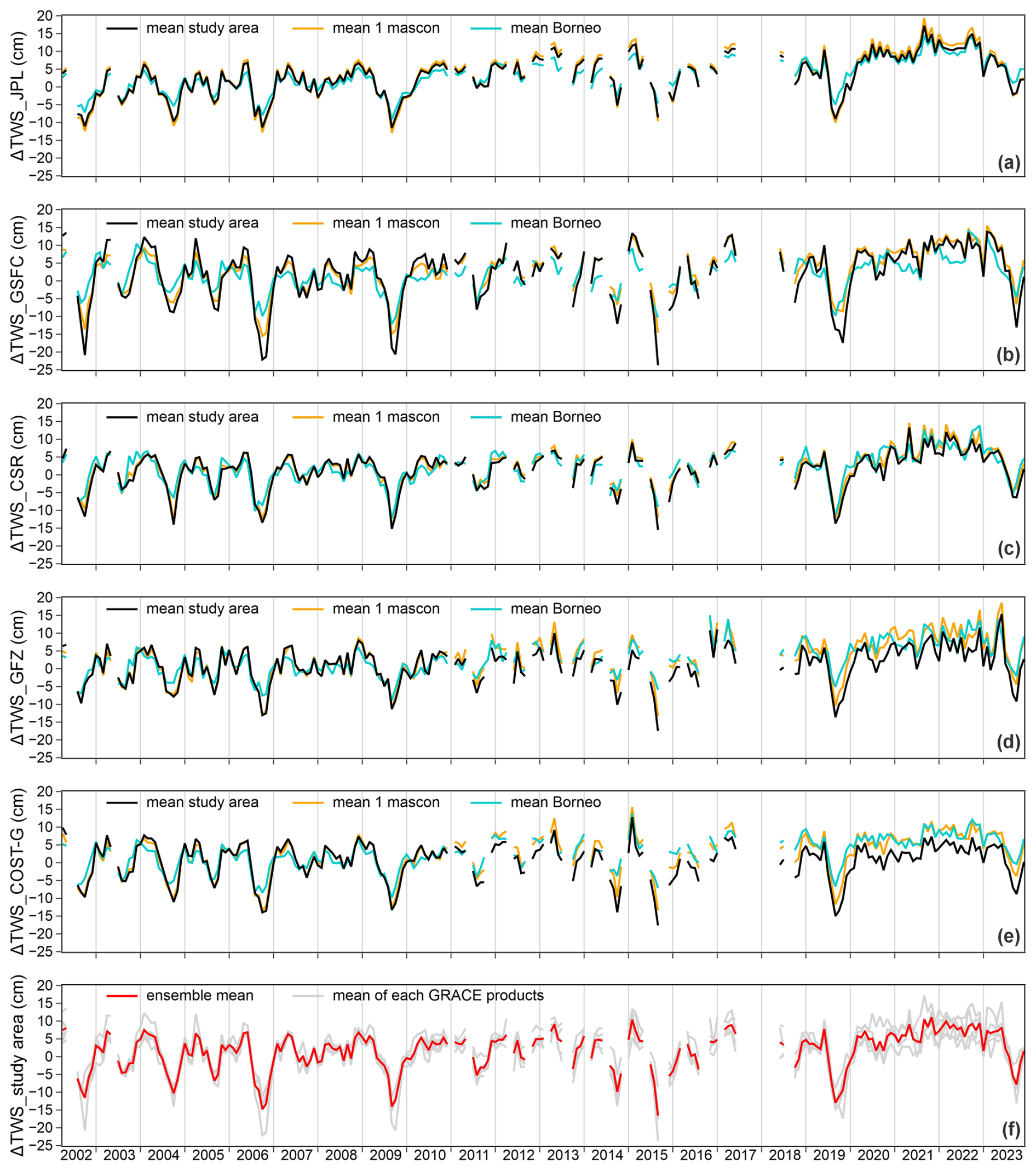
Figure 2 Comparison of mean ΔTWS values from different GRACE datasets: (a) JPL, (b) GSFC, (c) CSR, (d) GFZ, and (e) COST-G. In (a–e), the black, orange, and blue lines represent ΔTWS for the study area, a single 3° mascon, and the entire Borneo, respectively. Plot (f) shows the ensemble mean ΔTWS of the study area (red line) derived from the five GRACE datasets (gray lines). Missing ΔTWS data are indicated by gaps in the dataset.

3.2 Ocean leakage into inland GRACE signals

We evaluate how leakage from adjacent ocean grids may influence ΔTWS estimates in a small coastal basin that is below GRACE's effective footprint. This was assessed by pairing each Borneo land grid with the nearest ocean grid and computing correlations before and after detrending and de-seasonalizing using STL (Fig. S8 in the Supplement). Residual land-ocean correlations remain non-negligible and they differ by product. Within 100–150 km of the coast, CSR shows the highest median residual correlation (0.68; r²=0.46), whereas JPL (0.22; r²=0.05) and GSFC (0.17; r²=0.03) are much weaker. GFZ (0.43; r²=0.18) and COST-G (0.36; r²=0.13) fall in between. Inland (150–250 km), CSR weakens (0.42; r²=0.17) whereas GFZ (0.47; r²=0.22) and COST-G (0.42; r²=0.17) retain relatively moderate correlations that may reflect leakage and filtering artifacts. These results demonstrate that leakage effects are strongly product dependent, with CSR most affected near the coast and spherical harmonic products retaining inland correlations. These correlations represent, however, only an upper boundary since shared land-ocean variance may also reflect co-varying climate signals and ocean loading due to the non-unique nature of mass inversion (Heki and Jin, 2023; Ndehedehe and Ferreira, 2020; Chen et al., 2022; Chao, 2005). Identifying the relative contributions of different sources requires independent constraints from numerical modeling or alternative observational methods (Chen et al., 2022).

3.3 Simulated water storage components from GLDAS and WGHM

In the study area, water storage components derived from the GLDAS and WGHM datasets exhibit distinct contributions to mean ensemble ΔTWS. Among these components, soil moisture storage changes (ΔSMS) play the most dominant role with values ranging from $-\mathrm{28.8}-\mathrm{5.5}\mathrm{cm}$ (Table S4 and Fig. S9 in the Supplement). In contrast, surface water storage changes (ΔSWS) derived from the Noah LSM and WGHM datasets are comparatively smaller, ranging from $-\mathrm{5.3}-\mathrm{5.5}\mathrm{cm}$ (Table S4 and Fig. S1). Canopy water anomalies (ΔCW) are negligible with values ranging from $-\mathrm{0.02}-\mathrm{0.01}\mathrm{cm}$ (Table S4 and Fig. S10 in the Supplement). The very low ΔCW values indicate that canopy water variations have an insignificant influence on overall water storage changes, whereas small ΔSWS values suggest that surface water contributes minimally to ΔTWS in the study area.

Between the two GLDAS datasets, ΔSMS from Noah LSM exhibits greater variability and stronger negative skewness (−1.93) than Catchment LSM (−1.06). The pronounced skewness in Noah LSM ΔSMS indicates an asymmetric distribution with a higher frequency of extremely low values, suggesting that the Noah LSM is more responsive to extreme moisture deficits. Conversely, the skewness in the Catchment LSM reflects a more evenly distributed dataset with fewer extreme negative values, indicating a more stable soil moisture regime. These differences highlight the sensitivity of Noah LSM to extreme hydrological conditions, which may be advantageous for detecting short-term anomalies but could also introduce greater uncertainty when assessing long-term trends. Despite the dataset-specific variations, ΔSMS values from Noah and Catchment LSMs exhibit a strong positive correlation (r=0.86), indicating that both datasets capture similar trends in soil moisture variations over the study area. This high correlation suggests that although ΔSMS values may differ between models due to variations in parameterization and calibration, the overall patterns of soil moisture fluctuations remain consistent across both datasets.

ΔSWS was derived from WGHM and Noah LSM, ranging between $-\mathrm{1}-\mathrm{3.7}\mathrm{cm}$ for Noah and $-\mathrm{5.3}-\mathrm{5.5}\mathrm{cm}$ for WGHM. The broader range in WGHM reflects stronger variability in simulated surface water processes. Using bathymetry data from 15 lakes in the GLOBathy dataset (Khazaei et al., 2022) that represent major surface water bodies in the study area (Fig. S11 in the Supplement) together with surface water extent changes from Pekel et al. (2016), we estimated lake storage changes (ΔLS). ΔLS values are generally smaller than ΔSWS from both Noah and WGHM, ranging from $-\mathrm{1.6}-\mathrm{0.8}\mathrm{cm}$ (Fig. S12 in the Supplement). ΔLS from GLOBathy shows moderate agreement with WGHM-estimated ΔLS ($r=\mathrm{0.52};$ RMSE=0.1 cm) and ΔSWS from Noah (r=0.53; RMSE=0.1 cm) but a weaker agreement with ΔSWS from WGHM (r=0.12; RMSE=0.4 cm).

River storage changes could not be quantified because of the sparse river monitoring network (Schwatke et al., 2015). The global surface water dataset (Pekel et al., 2016) indicates that river areas in the LKB varied between 30 and 125 km² (mean ∼110 km²) between 2003 and 2021 (Fig. S12) whereas lake areas varied between 10 and 370 km² (mean ∼260 km²). These differences suggest that river storage changes were likely smaller than ΔLS, though this remains unverified due to lack of volume estimates. In addition, wetlands and peatlands surrounding the lakes in the northwest of the study area (Patria et al., 2025) may contribute to underestimation of ΔSWS. On average, lakes and rivers account for ∼77 % of the maximum surface water extent (Fig. S12), with wetlands and peatlands comprising the remaining ∼23 %. WGHM simulates negligible wetland storage variability (on the order of 10⁻² cm), indicating that current models may not adequately capture wetland and peatland dynamics.

3.4 ΔTWS and ΔSMS variability

Ensemble mean ΔTWS derived from the five GRACE datasets (JPL, GSFC, CSR, GFZ, and COST-G) exhibits substantial interannual variability from 2002–2023 (Fig. 2f). These fluctuations are characterized by alternating positive anomalies indicating increases in water storage, and negative anomalies signifying periods of water storage decline. The ensemble mean ΔTWS ranges from $-\mathrm{16.6}-\mathrm{11.1}\mathrm{cm}$.

Analysis of GRACE-derived annual ΔTWS trends within the study area provides insights into long-term hydrological changes. The 3° GRACE JPL mascon dataset reveals an annual ΔTWS trend of 0.6 cm yr⁻¹ at the single-mascon scale (Fig. 3a and 3e). At finer spatial resolutions, mean annual ΔTWS trends are of lower magnitudes: 0.5 cm yr⁻¹ for GRACE JPL (0.5° grids), 0.31 cm yr⁻¹ for GRACE GSFC (0.5° grids), 0.27 cm yr⁻¹ for GRACE CSR (0.25° grids), 0.26 cm yr⁻¹ for GRACE GFZ (1° grids), and 0.11 cm yr⁻¹ for GRACE COSTG (1° grids). Closer to the native resolution of GRACE, the 3° GRACE JPL mascon data reveal the strongest positive trend of 1.4 cm yr⁻¹ in the Sarawak region of Malaysia (Fig. 3a). This trend slightly decreases to 1.36 cm yr⁻¹ in the 0.5° ensemble of GRACE JPL, increases to 1.6 cm yr⁻¹ in the 0.5° ensemble of GRACE GSFC, 1.1 cm yr⁻¹ in both 1° ensembles of GRACE GFZ and COST-G, and is substantially lower at 0.51 cm yr⁻¹ in the 0.25° ensemble of GRACE CSR. Additionally, ΔTWS trend signals of each 0.5° grids within the study area (Fig. 3e) vary considerably across GRACE mascon datasets, reinforcing the recommendation to avoid single-grid-based analyses and instead employ ensemble mean values for more robust interpretations (Vishwakarma, 2020; Dahle et al., 2025).

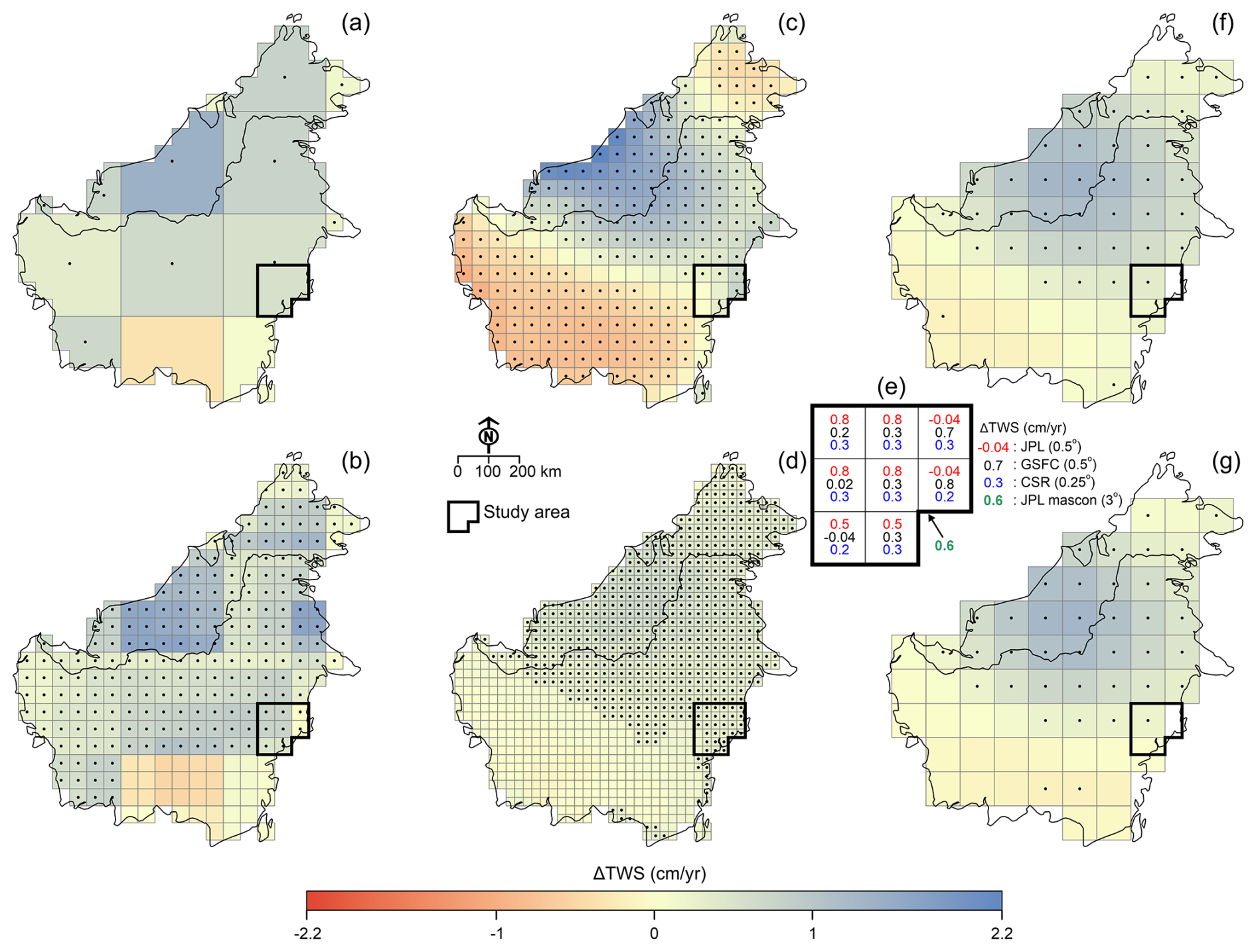
Figure 3 Comparison of GRACE datasets: (a) JPL (3° mascon grids), (b) JPL (0.5° grids), (c) GSFC (0.5° grids), (d) CSR (0.25° grids), (f) GFZ (1° grids), and (g) COST-G (1° grids). The maps display the annual trend of terrestrial water storage anomalies (ΔTWS) derived using the Theil–Sen method. Black dots indicate areas where p-values are <0.05, signifying statistical significance. Plot (e) displays the annual ΔTWS trends for each grid within the study area across GRACE mascon datasets.

The spatial distribution of ΔTWS signals across different grids within the study area reveals dataset-specific variability. The GRACE GSFC, CSR, GFZ, and COST-G datasets exhibit consistent ΔTWS patterns across all grids, whereas GRACE JPL shows localized discrepancies in two of the eight grids (Fig. S13 in the Supplement). These two grids remain relatively stable over time, showing minimal ΔTWS variations. Gain factor analysis of the GRACE JPL dataset (Fig. S14 in the Supplement) further highlights these differences: two grids within the JPL dataset have negative gain factors (−0.07), whereas the remaining six grids exhibit positive gain factors (0.83 and 1.4). Positive gain factors enhance ΔTWS variability, leading to ΔTWS patterns that closely match those from the other four GRACE datasets. Conversely, negative gain factors, particularly in the Mahakam Delta area, suppress ΔTWS fluctuations, resulting in significantly lower ΔTWS variability, ranging only from $-\mathrm{1.3}-\mathrm{0.9}\mathrm{cm}$ from 2002–2023 period. The dampening effect of negative gain factors suggests potential data filtering artifacts which may reduce GRACE sensitivity.

To investigate water storage variability, seasonal-trend decomposition using LOESS (STL) analysis is applied to ensemble mean ΔTWS values, revealing a nonlinear trend (Fig. S15 in the Supplement). Among the decomposed components, the residual component accounts for the highest ΔTWS variance (12.6 cm²), followed by seasonal (8.2 cm²) and trend (4.7 cm²) components. The dominance of the residual component suggests that short-term irregular ΔTWS fluctuations drive significant hydrological variability in the study area.

A similar pattern emerges when analyzing ΔSMS from GLDAS over the 2003–2023 period. Like ΔTWS, ΔSMS exhibits alternating positive and negative anomalies, representing soil moisture increases and deficits. STL analysis of mean ensemble ΔSMS values also reveals a nonlinear trend (Fig. S16 in the Supplement), with the residual component accounting for the highest variance (13.7 cm²), followed by seasonal (5.1 cm²) and trend (1.1 cm²) components. These results confirm that soil moisture fluctuations are the primary driver of short-term terrestrial water storage variability in the study area, reinforcing the dominant role of ΔSMS in controlling overall ΔTWS dynamics.

3.5 ΔGWS estimates

As a residual parameter (Eq. 1), ΔGWS is subject to propagated errors and uncertainties from filtered GRACE ΔTWS and global-scale models used in its computation (Vishwakarma et al., 2016), which can lead to arithmetic problems as pointed out by Shamsudduha and Taylor (2020) and Arifin et al. (2025b). Simulations from global-scale models have limitations in their ability to represent accurately changes in individual terrestrial stores (e.g. ΔSMS, ΔSWS) as highlighted, for example, by their inferred collective comparison with GRACE ΔTWS (Scanlon et al., 2018). Discrepancies in individual stores (e.g. ΔSMS) can directly influence computation of GRACE ΔGWS from GRACE ΔTWS.

Figure 4 shows that when ΔSMS values from Noah LSM are more negative than ΔTWS values from GRACE JPL (0.5°), GRACE ΔGWS becomes anomalously high and vice versa. For example (Table 1), during the wet season, ΔTWS in March 2008 was 1.9 cm, whereas ΔSMS was 5 cm and ΔSWS was 3.6 cm. The computed ΔGWS of −6.7 cm is implausible unless intense and widespread groundwater abstraction has occurred. Conversely, in September 2015 when precipitation was zero, ΔTWS was −8.6 cm, ΔSMS was −22.5 cm, and ΔSWS was −4.1 cm. Despite the overall water deficit, the computed ΔGWS was 18 cm, an implausible gain unless significant regional groundwater inflow into the GRACE grid occurred. These examples highlight computational uncertainty in ΔGWS estimation, particularly when specific dataset combinations are used.

We tested 54 realizations to compute ΔGWS from 2003–2023 using six ΔTWS datasets (JPL, GSFC, CSR, GFZ, COST-G and the ensemble mean), three ΔSMS datasets (Noah LSM, Catchment LSM, and the ensemble mean), and three ΔSWS datasets (WGHM, Noah LSM, and the ensemble mean). Eight criteria (Table S5 in the Supplement), developed by Arifin et al. (2025b) for global tropical regions, were applied to identify physically plausible ΔGWS values within ΔTWS bounds. We find that plausible GRACE-derived ΔGWS estimates per realization range from 21 %–60 % (mean=42 %). Filtering for plausible realizations improved consistency with 87 % of ensemble mean ΔGWS values suitable for further analysis (Fig. 5). Implausible values mainly arose: (1) in wet periods, when ΔSMS+ΔSWS exceeded ΔTWS, yielding negative ΔGWS, and (2) in dry periods, when $|\mathrm{\Delta }\text{SMS}+\mathrm{\Delta }\text{SWS}|$ exceeded $\left|\mathrm{\Delta }\text{TWS}\right|$, producing anomalously positive ΔGWS. Implausible ΔGWS estimates may reflect propagated errors due to ocean signal leakage in GRACE-derived ΔTWS and inconsistencies between GRACE observations and model-simulated components.

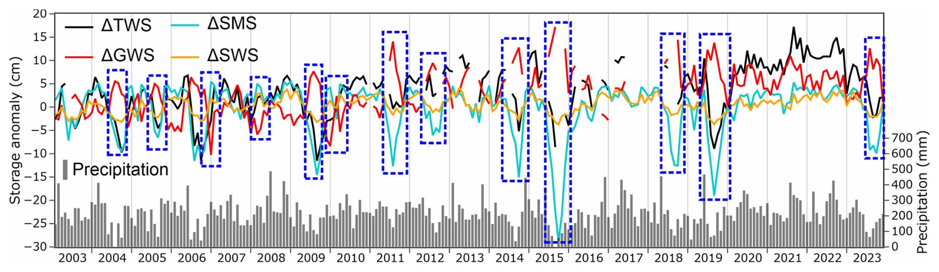
Figure 4 Comparison between mean ΔTWS (GRACE JPL 0.5°), ΔSMS (Noah LSM), ΔSWS (WGHM), and computed ΔGWS. Blue dashed polygons indicate arithmetic problems resulting from ΔSMS values being significantly lower than ΔTWS.

Table 1 Examples of arithmetically implausible ΔGWS estimates based on the comparison between mean ΔTWS (GRACE JPL 0.5°), ΔSMS (Noah LSM), and ΔSWS (WGHM).

The ensemble mean of plausible ΔGWS ranges from −4.5–7.2 cm with an annual trend of 0.2 cm yr⁻¹ (p<0.05), whereas incorporating implausible values results in ΔGWS ranges between −5.6 and 8.7 cm with an annual trend of 0.02 cm yr⁻¹ (p>0.05). STL decomposition (Fig. S17 in the Supplement) shows residual variance dominates (2.2 cm²), followed by trend (1.7 cm²) and seasonal (0.8 cm²) components. Ensemble mean ΔGWS correlates strongly with ΔTWS (r=0.86), but inclusion of implausible values significantly reduces the correlation to 0.12 (Fig. 6). We further compared ΔGWS from this study with the Global Land Water Storage (GLWS 2.0) and GLDAS 2.2 datasets. Plausibility checks indicate 45 %–65 % (mean=54 %) of GLWS 0.5° estimates and 88 %–99 % (mean=95 %) of GLDAS 0.25° estimates are consistent with ΔTWS bounds. Ensemble means yielded 93 % (GLWS) and 100 % (GLDAS) plausible estimates. ΔGWS values from both datasets correlate strongly with ΔTWS ($r=\mathrm{0.70}-\mathrm{0.99}$) though including implausible values reduces GLWS correlations to 0.63 (Fig. 6). Notably, both datasets exhibit much higher ΔGWS variability than our ΔGWS estimates (Fig. 6g): $-\mathrm{23.3}-\mathrm{25.4}\mathrm{cm}$ for GLWS (trend $-\mathrm{0.5}\mathrm{cm}{\mathrm{yr}}^{-\mathrm{1}}$, p=0.2) and $-\mathrm{37.8}-\mathrm{6.2}\mathrm{cm}$ for GLDAS (trend $-\mathrm{0.7}\mathrm{cm}{\mathrm{yr}}^{-\mathrm{1}}$, p<0.05).

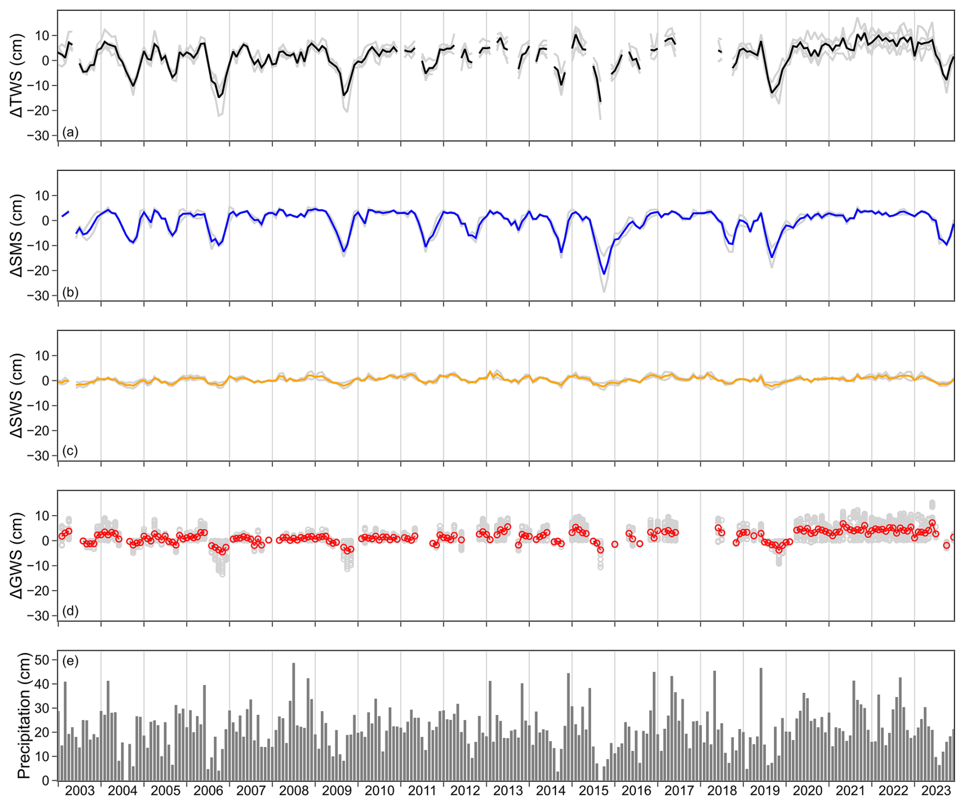
Figure 5 Ensemble mean of (a) ΔTWS (black line), (b) ΔSMS (blue line), and (c) ΔSWS (orange line). Plot (d) shows arithmetically plausible mean ΔGWS (red line and circles) from 54 realizations (gray circles). Plot (e) shows monthly precipitation. Gray lines in (a, b) represent ΔTWS and ΔSMS from individual GRACE and GLDAS datasets. In (c), gray lines indicate ΔSWS from the Noah LSM and WGHM datasets.

3.6 The influence of climate variability on water storage changes

Correlations between ΔTWS, ΔSMS, and ΔGWS and four major climate indices (MEI, ONI, DMI, PDO) as well as precipitation in the study area were computed to evaluate the sensitivity of water storage changes to large-scale climatic forcing (Fig. S18 in the Supplement). The rationale is that large-scale climate modes, particularly ENSO, exert a dominant influence on terrestrial water storage variability across Indonesia (Liu et al., 2020) and therefore provide a benchmark to test whether GRACE-derived water storage changes capture physically meaningful variability.

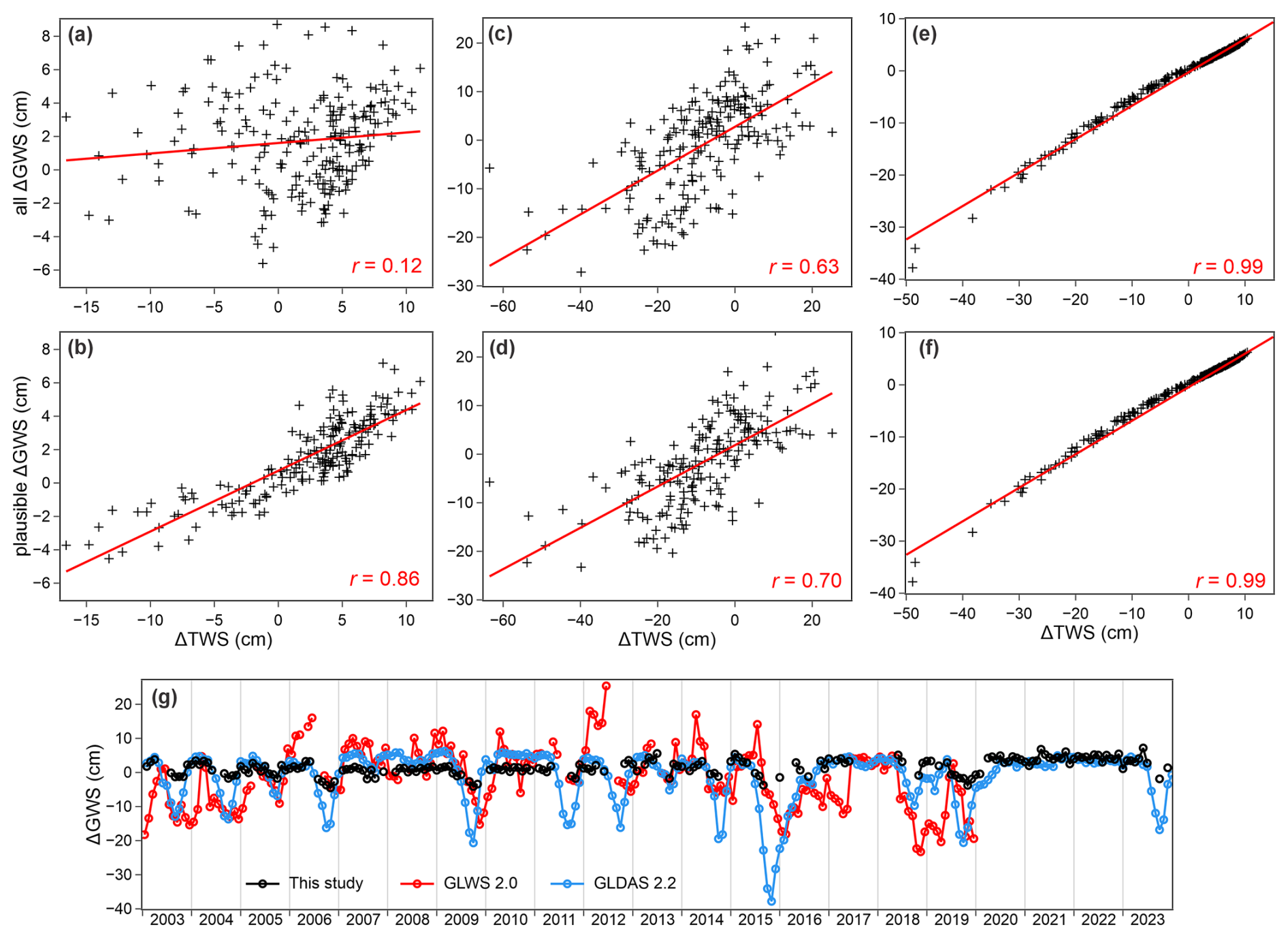
Figure 6 Cross-correlations between ensemble mean ΔTWS and ΔGWS from (a, b) this study, (c, d) the GLWS dataset, and (e, f) the GLDAS dataset with and without implausible estimates; (g) comparison of ΔGWS from this study and GLWS.

Across GRACE products, ΔTWS shows weak-to-moderate correlations (p-value<0.05) with ENSO indices, with r values ranging from −0.46 to −0.56 for MEI and −0.41 to −0.48 for ONI. Ensemble mean ΔTWS yields correlations of −0.52 (MEI) and −0.46 (ONI) whereas weaker correlations are observed with the IOD (DMI, $r=-\mathrm{0.26}$) and PDO ($r=-\mathrm{0.25}$). These results indicate that ENSO is the dominant driver of ΔTWS variability in the study area compared to IOD and PDO.

ΔSMS exhibits slightly stronger ENSO sensitivity than ΔTWS. Catchment and Noah LSMs yield r values with MEI and ONI ranging from −0.56 to −0.62 whereas the ensemble mean shows correlations of −0.60 (MEI) and −0.61 (ONI) with p-value<0.05. As with ΔTWS, correlations with DMI (−0.31 to −0.35) and PDO (−0.2 to −0.22) are weaker. These suggest that soil moisture anomalies are relatively sensitive to ENSO events. Monthly precipitation also correlates moderately with ΔTWS ($r=\mathrm{0.47}-\mathrm{0.52}$) and ΔSMS ($r=\mathrm{0.46}-\mathrm{0.58}$).

Correlations between ensemble mean plausible ΔGWS in this study with climate indices or precipitation remain consistently weaker than those for ΔTWS or ΔSMS, with values of −0.41 (MEI), −0.33 (ONI), −0.18 (DMI), −0.23 (PDO), and 0.38 (precipitation) with p-value<0.05. The ensemble mean plausible ΔGWS estimates from GLWS datasets are similar, with values of −0.44 (MEI), −0.48 (ONI), −0.17 (DMI), −0.26 (PDO), and 0.29 (precipitation). In contrast, the GLDAS dataset exhibits substantially stronger correlations with MEI (−0.6) and ONI (−0.63), whereas correlations with other indices are relatively comparable: −0.32 (DMI), −0.21 (PDO), and 0.43 (precipitation). In addition, we repeated the correlation analysis using de-seasonalized and detrended components of ΔTWS, ΔSMS, and ΔGWS which resulted in generally weaker correlations than those of the raw data (Fig. S19 in the Supplement). This reduction indicates that much of the ENSO-related signal is expressed through modulation of the seasonal cycle of water storage changes rather than non-seasonal anomalies.

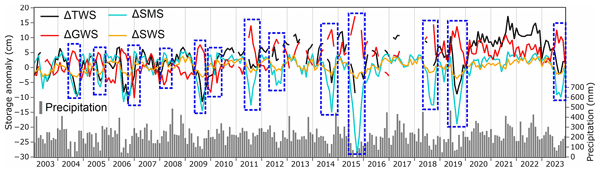
Although overall correlations between ENSO indices, ΔTWS, and ΔSMS are weak-to-moderate ($r=-\mathrm{0.4}$ to −0.6), the impact of strong ENSO events is much more pronounced, particularly during extreme El Niño and La Niña phases. This is indicated by strongly positive or negative ONI values exceeding ±0.5 °C for at least five consecutive months, accompanied by corresponding sustained positive or negative MEI values. These strong ENSO events coincide with the most extreme ΔTWS and ΔSMS fluctuations in the study area (Fig. 7). A notable example is the 2015–2016 El Niño, recognized as one of the strongest on record (L'Heureux et al., 2017). This event resulted in record-low ΔTWS and ΔSMS estimates, indicating severe terrestrial water deficits likely driven by widespread drought conditions, as also reflected in strong negative SPEI values (Fig. 7d). The ΔTWS and ΔSMS responses during this extreme El Niño underscore the sensitivity of water storage components to large-scale climatic forcing, particularly ENSO.

4 Discussion

4.1 Comparison of GRACE-derived ΔGWS with in situ piezometric observations

A key challenge in using GRACE to monitor groundwater dynamics is its coarse spatial resolution (≥90 000 km²), which restricts its ability to resolve localized groundwater level fluctuations (Loomis et al., 2021; Tapley et al., 2004; Shamsudduha and Taylor, 2020; Wiese et al., 2016; Alley and Konikow, 2015). Consequently, ΔGWS estimates may deviate substantially from in situ piezometric observations, particularly in regions where localized factors such as groundwater abstraction introduce variability (Shamsudduha and Taylor, 2020; Asoka et al., 2017).

In the Bengal Basin (∼138 000 km²), which shares a similar coastal deltaic setting as the LKB, ΔGWS estimates derived from a dense network of monitoring wells exhibit a strong correlation with GRACE-based ΔGWS (Shamsudduha et al., 2012). In other regions however, GRACE-based ΔGWS align less well with observed values. For example, Asoka et al. (2017) reported that GRACE-derived ΔGWS trends in India underestimated those derived from piezometric data, likely due to localized depletion not captured at GRACE's coarse resolution. Similarly, Shamsudduha and Taylor (2020) reported increasing GRACE-derived ΔGWS trends in the Guarani Aquifer System (South America) despite observed groundwater depletion caused by intensive urban and agricultural groundwater withdrawals during the same period.

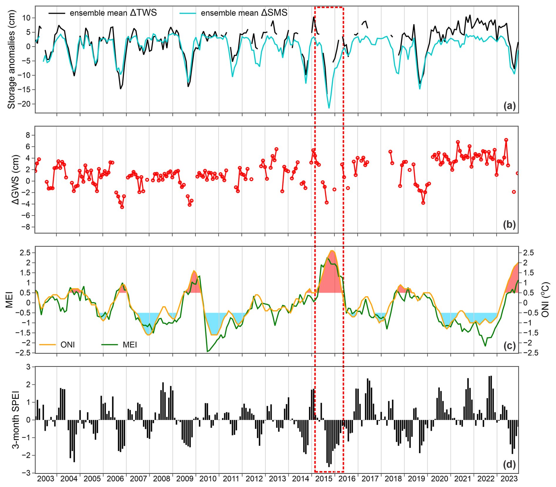
Figure 7 Comparison of (a) ensemble mean ΔTWS and ΔSMS, (b) ensemble mean ΔGWS, (c) MEI and ONI indices, and (d) 3 month SPEI. In (c), red and blue shadings represent El Niño and La Niña episodes respectively, where ONI exceeds ±0.5 °C. The strongest recorded El Niño event (2015/2016) is highlighted by a red dashed polygon.

In the study area, groundwater abstraction is concentrated within ∼20 km of coast, particularly south of Balikpapan City. We compared ensemble mean plausible GRACE-derived ΔGWS with groundwater level changes (ΔGWL) as the storage coefficient (S or S_y) is not well constrained. Lithological logs reveal heterogeneous interbedded sand and clay units (Fig. S20 in the Supplement; Arifin et al., 2024). Piezometer depths range from 21–135 m; shallow screens up to ∼40 m may represent unconfined aquifers whereas deeper screens may tap confined aquifers. In similar deltaic settings such as the Mekong and Indo-Gangetic deltas, storage coefficients mostly vary from $\sim \mathrm{0.08}-\mathrm{0.25}$ (mean ∼0.15) for unconfined aquifers and from $\sim {\mathrm{10}}^{-\mathrm{5}}-\mathrm{8}\times {\mathrm{10}}^{-\mathrm{4}}$ (mean $\sim \mathrm{5}\times {\mathrm{10}}^{-\mathrm{4}}$) for confined aquifers (BGS and DPHE, 2001; Bonsor et al., 2017; Van et al., 2023; Pechstein et al., 2018). This uncertainty translates into a range of possible ΔGWS values (Fig. 8). On average, confined aquifers yield ∼0.5 mm of storage loss per metre of decline ($S=\mathrm{5}\times {\mathrm{10}}^{-\mathrm{4}}$), whereas unconfined aquifers yield ∼15 cm (S_y=0.15). Although correlations are less sensitive to amplitude uncertainty, the magnitude and trend of GRACE-derived ΔGWS in a small, data-scarce basin such as the LKB remain highly uncertain due to leakage effects, error propagation in the residual calculation, and the lack of both a reliable storage coefficients and dense piezometric network. As a result, the minimum detectable ΔGWS signal cannot be clearly quantified.

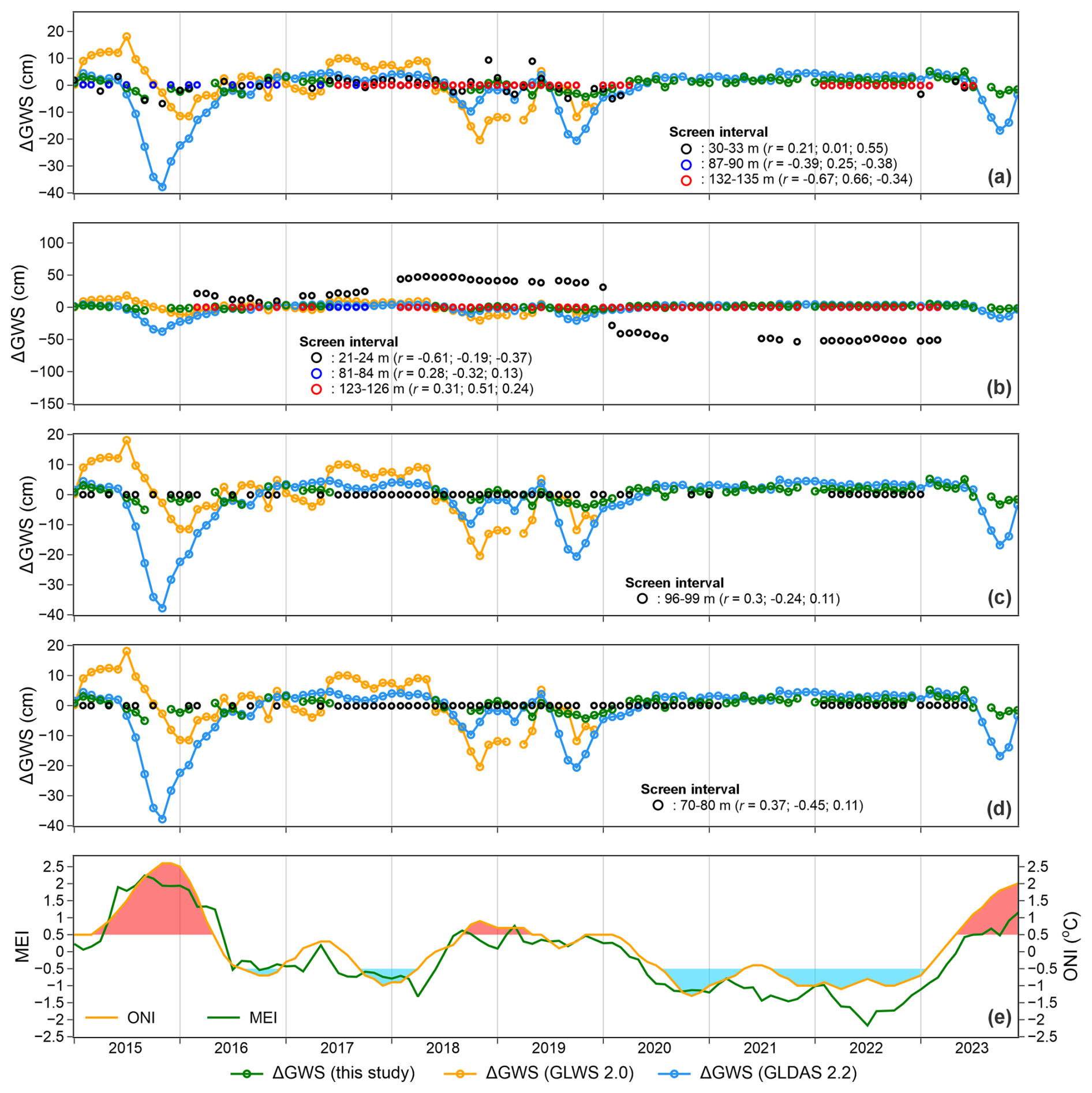
Figure 8 Comparison between ΔGWS from piezometers (black, dark blue, and red circles) at (a) MG, (b) MM, (c) GM, and (d) TS sites with GRACE-derived ΔGWS (green, orange, and light blue circle-line); (e) MEI (green line) and ONI (orange line) indices. All ΔGWS values are referenced to the 2015–2023 mean baseline. Correlation coefficients (r) are reported: the first indicates correlation between piezometric ΔGWS and GRACE-derived ΔGWS from this study, the second with GLWS-derived ΔGWS, and the third with GLDAS-derived ΔGWS. In (e), red and blue shadings represent El Niño and La Niña episodes, respectively, where ONI exceeds ±0.5 °C.

Correlations between GRACE-based ΔGWS and ΔGWL vary substantially across sites and screened intervals. At MG (30–33 m), ΔGWS from this study correlates weakly with ΔGWL (r=0.21), whereas ΔGWS from the GLDAS dataset shows a stronger correlation (r=0.55) and GLWS shows nearly none (r=0.01). At deeper intervals in MG (87–90 m; 132–135 m), ΔGWS from this study is negatively correlated with ΔGWL ($r=-\mathrm{0.39}$ to −0.67), indicating a decoupling between regional storage dynamics and local aquifer responses. GLDAS-based ΔGWS also shows negative correlations (−0.38 to −0.34), whereas GLWS yields positive correlations (0.25–0.66), underscoring dataset-dependent discrepancies. These mismatches indicate that GRACE-derived ΔGWS may reflect regional-scale storage dynamics in the study area that contrast with piezometric observations representing localized responses influenced by aquifer heterogeneity and groundwater abstraction.

In several instances, piezometric observations show ΔGWL trends that differ from ΔGWS signals (Fig. S21 in the Supplement). At site MG (screened interval: 87–135 m), ΔGWL exhibits a continuous decline from 2015–2023, with rates of $-\mathrm{0.9}\mathrm{m}{\mathrm{yr}}^{-\mathrm{1}}$ (p<0.05) for the 87–90 m interval and $-\mathrm{0.6}\mathrm{m}{\mathrm{yr}}^{-\mathrm{1}}$ (p-value<0.05) for the 132–135 m interval. Similarly, at site MM (screened interval: 21–24 m), ΔGWL dropped significantly from 5.1–0.1 m by the end of 2019, followed by a relatively stable trend through 2023. These discrepancies may be attributable to localized groundwater abstraction, which can play a dominant role in influencing local groundwater level changes from piezometry and override regional-scale ΔGWS trends observed from GRACE data.

The GRACE-based ΔGWS trend of 0.2 cm yr⁻¹ (p<0.05) over the last two decades may indicate an aquifer-full condition in the study area. This interpretation is supported by intra-annual ΔTWS patterns, which display substantial declines during periods of low precipitation but rapid recoveries following increases in rainfall (Figs. 5 and 7). Additional evidence is provided by groundwater level observations at the MG site (screened interval: 30–33 m), where water levels have remained very shallow, fluctuating between 0.3 and 1.4 m b.g.l. from 2015–2023, with a mean of 1.0±0.1 m. Groundwater abstraction is not regional but largely concentrated near the southern coast of Balikpapan City, likely contributing to localized declines in groundwater levels.

4.2 ENSO influence on water storage variability

This study identifies weak-to-moderate correlations between ENSO indices (MEI and ONI), ΔTWS, and ΔSMS with r values ranging from −0.41 to −0.62, indicating that ENSO events exert a substantial influence on water storage variability in the study area. Correlations between ΔTWS and ΔSMS with monthly precipitation are similar in magnitude (0.47−0.58). In contrast, ΔGWS exhibits weaker responses, with correlations of −0.41 (MEI), −0.33 (ONI), and 0.38 (precipitation). No significant lag effect is detected; introducing 1- to 6-month lags consistently weakens correlations (Fig. S22 in the Supplement). For instance, the correlation between MEI and ensemble mean ΔTWS declines from −0.49 at a 1-month lag to −0.17 at a 6-month lag, suggesting that water storage anomalies in the study area respond contemporaneously to ENSO variability. This aligns with previous findings which reported no significant lag between ΔTWS and ENSO-related teleconnection indices across most of Indonesia (Liu et al., 2020), which may be consistent with an aquifer-full condition in the study area.

Plots of ensemble mean ΔTWS, ΔSMS, and ΔGWS alongside ENSO indices (MEI, ONI) and the 3 month SPEI (Fig. 7) further confirm a strong correlation between water storage anomalies and ENSO events in the study area. Documented El Niño events in 2004, 2006, 2009, 2015/2016, 2018/2019, and 2023 (Kamra and Athira, 2016; McPhaden, 2004; Lee et al., 2020; Raghuraman et al., 2024) coincide with negative SPEI values, indicative of pronounced dry conditions during these periods. Among these, the 2015–2016 El Niño stands out as one of the most intense El Niño episodes in recent decades, leading to severe drought across Southeast Asia and increased forest fires in Indonesia (Santoso et al., 2017; Kogan and Guo, 2017; L'Heureux et al., 2017).

During the February–October 2015 El Niño period, water storage anomalies in the study area exhibited significant negative trends. ΔTWS decreased between −2.4 and $-\mathrm{4.6}\mathrm{cm}{\mathrm{month}}^{-\mathrm{1}}$ across GRACE products, with the ensemble mean at $-\mathrm{2.9}\mathrm{cm}{\mathrm{month}}^{-\mathrm{1}}$. Similarly, ΔSMS decreased from $-\mathrm{2.2}\mathrm{cm}{\mathrm{month}}^{-\mathrm{1}}$ (Catchment) to $-\mathrm{4.1}\mathrm{cm}{\mathrm{month}}^{-\mathrm{1}}$ (Noah), with an ensemble mean of $-\mathrm{3.2}\mathrm{cm}{\mathrm{month}}^{-\mathrm{1}}$. The plausible ΔGWS from this study also showed a significant decline of $-\mathrm{1.1}\mathrm{cm}{\mathrm{month}}^{-\mathrm{1}}$ (p<0.05). Similar responses have been observed in other regions. Southern Africa experienced severe drought and water storage depletion during the 2015–2016 El Niño, whereas Eastern Africa experienced anomalously wet conditions, leading to increases in ΔTWS and groundwater recharge as observed in both GRACE data and in situ piezometric records (Kolusu et al., 2019; Scanlon et al., 2022).

The transition to La Niña phases, such as the 2010 event, one of the strongest La Niña episodes in recent history (Boening et al., 2012), led to significant increases in water storage in the study area. Between September 2009 and June 2010, positive trends were observed: ΔTWS increased by 1.5–3 cm month⁻¹ across GRACE products, whereas ΔSMS increased by 1.6 cm month⁻¹ in both Noah and Catchment LSMs, all statistically significant (p<0.05). In contrast, plausible ΔGWS exhibited a weaker increasing trend of 0.7 cm month⁻¹ ($p=\mathrm{0.06}).$ These trends confirm that La Niña events promote recharge effectively counteracting the deficits induced by preceding El Niño events.

Although GRACE-derived ΔGWS provides a valuable large-scale perspective on groundwater storage changes, piezometric data from monitoring wells offer localized insights into aquifer responses to ENSO variability. Groundwater-level changes (ΔGWL) from the GM and TS sites (Fig. S21) confirm that the 2015–2016 El Niño event was associated with significant groundwater-level declines of $-\mathrm{13.1}\mathrm{cm}{\mathrm{month}}^{-\mathrm{1}}$ (GM) and $-\mathrm{6.8}\mathrm{cm}{\mathrm{month}}^{-\mathrm{1}}$ (TS). Following this water storage depletion phase, a notable recharge event occurred in 2017, coinciding with the transition to La Niña conditions which facilitated moisture recovery in soils and aquifers. Similarly, the 2020–2022 La Niña events (Shi et al., 2023), typically associated with wetter conditions in Southeast Asia (Feng and Wang, 2018), coincide with increased ΔTWS, ΔSMS, and ΔGWS (Fig. 7). Piezometric records at MM and TS show corresponding upward trends (10–40 cm month⁻¹), reinforcing the role of La Niña in replenishing regional water resources. These underscore the dynamic relationship between ENSO phases and terrestrial water storage components in the study area. El Niño events lead to significant reductions in ΔTWS and ΔSMS, resulting in drought conditions and lower groundwater recharge rates whereas La Niña events promote water storage recovery, characterized by increases in precipitation, soil moisture retention, and groundwater recharge.

4.3 Uncertainty in GRACE-based ΔTWS and ΔGWS estimates

The GRACE JPL (3°), GFZ (1°), and COST-G (1°) datasets employed in this study provide uncertainty estimates for ΔTWS (Boergens et al., 2020, 2019, 2022; Dahle et al., 2025; Wahr et al., 2006). The mean uncertainty for the GRACE JPL mascon encompassing the study area is $\sim \mathrm{2.2}\pm \mathrm{1}\mathrm{cm}$, whereas GRACE GFZ and COST-G exhibit uncertainties of 2.2±0.7 and 1.4±0.4 cm, respectively (Fig. S23 in the Supplement). Uncertainty estimates at finer resolutions (0.5°–0.25°) are unavailable and are expected to be higher due to greater variability at smaller spatial scales (Landerer and Swenson, 2012). The absence of refined uncertainty quantifications at sub-mascon scales poses a limitation for ΔGWS assessments in localized settings as hydrological variability increases with decreasing spatial scale, making ΔGWS more sensitive to data noise and model parameterization errors.

As noted earlier, two of the eight 0.5° GRACE JPL grids within the study area exhibit negative gain factors (−0.07, Fig. S14), resulting in systematically lower ΔTWS magnitudes over time (Fig. S13a). This dampening effect is not observed in other GRACE datasets and is likely caused by oceanic signal interference with terrestrial water storage (Landerer and Swenson, 2012). In coastal areas such as the Mahakam Delta, the proximity to ocean masses can introduce filtering effects that suppress ΔTWS variability, reducing observed fluctuations. As a result, in areas dominated by negative gain factor grids, ΔSMS arithmetically becomes the primary driver of ΔTWS variability, which can lead to overestimation or underestimation of ΔGWS as the residual parameter.

Computational uncertainty in GRACE-derived ΔGWS arises due to its estimation as a residual component derived from the difference between GRACE-based ΔTWS and simulated water storage components (Eq. 1). Since ΔGWS is not directly measured by satellites but inferred through hydrological balance calculations, its accuracy depends on the reliability of ΔTWS estimates and the simulated water components in the study area, primarily ΔSMS and ΔSWS, which can propagate errors into ΔGWS estimates. However, these simulated components are not locally calibrated as soil moisture, river stage, and lake volume observations are largely unavailable.

As discussed in Sect. 3.2, ΔSMS exerts the most substantial influence on ΔTWS in this study, whereas ΔSWS contributes minimally, and ΔCW contributions are negligible (Table S4). Because ΔGWS is computed as a residual, any discrepancy between ΔTWS and ΔSMS directly affects ΔGWS estimations (Shamsudduha and Taylor, 2020; Arifin et al., 2025b). A key observation in Fig. 4 highlights that when ΔSMS values are lower than ΔTWS, ΔGWS estimates become anomalously high. It emphasizes the importance of obtaining reliable root zone soil moisture estimates as it represents the hydrologically active layer that exchanges water with both the atmosphere and the underlying unsaturated zone (Gao et al., 2024).

Another major source of uncertainty in GRACE-derived ΔGWS calculations is the representation of surface water storage and anthropogenic influences in the study area, including groundwater abstraction within the study area in the GLDAS and WGHM datasets. Notably, ΔSWS in GLDAS is not a direct measure of surface water storage but rather a simulation of surface runoff (Beaudoing and Rodell, 2020; Rodell et al., 2004; Li et al., 2019). This distinction is critical because surface runoff estimates do not account for water bodies (rivers, lakes, reservoirs, and wetlands), potentially leading to an underestimation of total ΔSWS contributions to ΔTWS (Scanlon et al., 2019; Getirana et al., 2017; Shamsudduha et al., 2012; Proulx et al., 2013). This limitation is particularly relevant in tropical regions such as the Amazon Basin where surface water storage contributes up to ∼27 % of total ΔTWS variations (Getirana et al., 2017).

In the present study, mean ΔSWS estimates from the Catchment LSM are significantly higher (−10.7–20.3 cm) than those from the WGHM and Noah LSM, which range from $-\mathrm{5.3}-\mathrm{5.5}\mathrm{cm}$ (Fig. S1). This discrepancy reinforces that using ΔSWS from the Catchment LSM could introduce substantial uncertainty into ΔGWS calculations. In contrast, ΔSWS from WGHM and Noah LSM appear more representative and are further supported by lake storage changes (ΔLS) derived from bathymetry of 15 lakes in the GLOBathy dataset (Khazaei et al., 2022) and surface water extent changes from Pekel et al. (2016). ΔLS values show relatively good agreement with ΔSWS from Noah LSM (RMSE=0.1 cm) and WGHM (RMSE=0.4 cm). Although river storage changes cannot be quantified directly due to sparse monitoring (Schwatke et al., 2015), the global surface water dataset (Pekel et al., 2016) suggests that river storage changes may be smaller than ΔLS and thus contribute less to ΔSWS than lakes. In addition, the lack of robust estimates for changes in wetlands and peatlands storage may lead to an underestimation of ΔSWS as these systems account for ∼23 % of surface water extent changes.

Across the 54 realizations tested in this study, ∼42 % of GRACE-derived ΔGWS estimates per realization are implausible, typically appearing as negative values during wet periods when all components are positive, or positive values during dry periods when all components are negative. Including implausible values reduces the correlation between ΔGWS and ΔTWS from 0.86–0.12 (Fig. 6a and b). The implausible values may not be merely computational anomalies but rather symptoms of poor or inconsistent input data, particularly where modeled ΔSMS and ΔSWS diverge from GRACE-observed ΔTWS (Scanlon et al., 2018). Therefore, this study emphasizes the importance of removing implausible water storage components from subsequent analyses as their inclusion could introduce significant bias and errors into hydrological interpretations and climate-groundwater assessments.

4.4 The role of extreme rainfall in groundwater recharge

This study finds weak-to-moderate correlations between ΔTWS, ΔSMS, and monthly precipitation averaged from Balikpapan and Samarinda stations. Correlation coefficients between ΔTWS and precipitation range from 0.47–0.52 (Fig. S18), whereas slightly higher values are observed between ΔSMS and precipitation ($r=\mathrm{0.49}-\mathrm{0.58}$). Introducing a 1 month lag does not significantly alter these values. In contrast, longer lags lead to a substantial decrease in correlation, dropping to ∼0.1 for both ΔTWS and ΔSMS at a 4 month lag (Fig. S22). These correlations suggest a relatively strong coupling with minimal lag effects between precipitation inputs and terrestrial water storage in the study area, particularly in near-surface soil moisture storage dynamics. This may indicate rapid infiltration of rainfall into the upper soil layers, likely due to limited water retention capacity in the vadose zone or the presence of highly permeable soils.

The ensemble mean plausible ΔGWS shows a weaker correlation with precipitation (r=0.38) compared to ΔTWS and ΔSMS. Introducing 1 month lag does not alter the correlation, whereas longer lags lead to a consistent decline, with r=0.16 at a 4 month lag. Despite the weak correlation between ΔGWS and precipitation, piezometric data reveal the important role of extreme rainfall events in groundwater recharge in the study area. The comparison between hourly piezometric data and daily precipitation (Fig. 9) confirms relatively rapid groundwater replenishment, driven by extreme rainfall events.

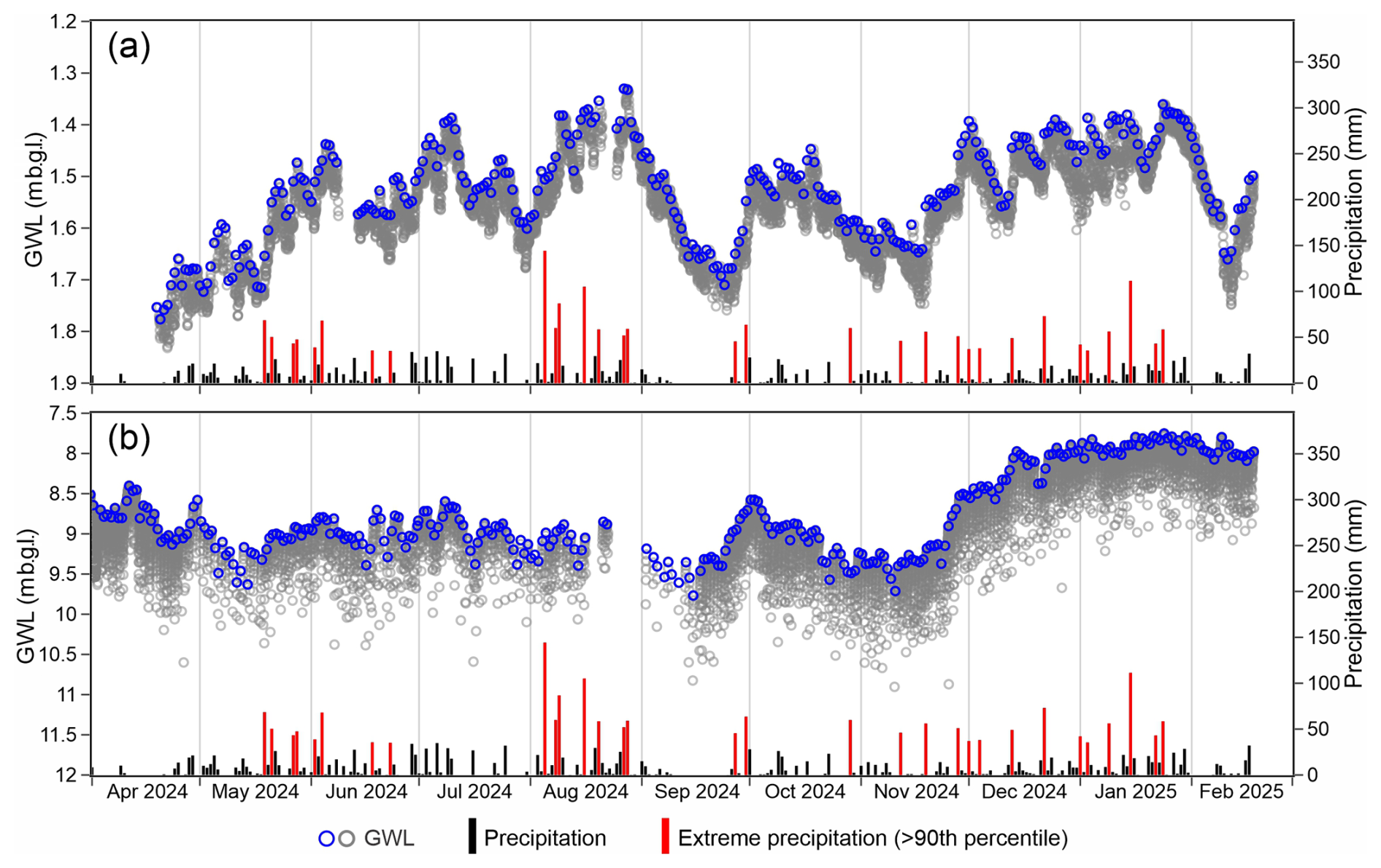
Figure 9 Comparison of hourly groundwater level (GWL) with daily precipitation from Balikpapan station at two monitoring sites: (a) MG site (screened interval: 30–33 m) and (b) EBD site (screened interval: 73–98 m). Blue circles represent the minimum GWL recorded per day. In (b), gray circles denote recovery data, whereas blue circles indicate the minimum GWL per day.

The contribution of high-intensity precipitation to groundwater recharge has been widely documented in recent studies (Shamsudduha and Taylor, 2020; Taylor et al., 2013a; Cuthbert et al., 2019b; Jasechko and Taylor, 2015; Goni et al., 2021; Seddon et al., 2021; Jasechko, 2019). Observations from April 2024–February 2025 indicate that extreme daily precipitation events exceeding the 90th percentile (>35 mm) are consistently followed by groundwater level rises (Fig. 9), reinforcing the notion that episodic high-intensity rainfall contributes to groundwater recharge in the study area. This evidence underscores the critical role of extreme rainfall events in groundwater recharge, suggesting that increased rainfall due to climate change (Taylor et al., 2013b) may enhance future groundwater recharge in the study area.

4.5 Challenges in groundwater monitoring and the potential of pumping well data

Establishing an extensive groundwater monitoring network in Indonesia including the study area is required to advance the renewability of groundwater withdrawals, particularly as many global aquifers experience rapid depletion (Jasechko et al., 2024; Taylor, 2014). An extensive monitoring system would facilitate early detection of depletion trends, inform water resource planning and support evidence-based policy decisions to prevent overabstraction. This is especially important in regions where geological heterogeneity and anthropogenic influences such as groundwater abstraction lead to significant groundwater level variations that are not well captured by large-scale GRACE ΔTWS and associated estimates of ΔGWS. Although the integration of GRACE ΔTWS with the estimation of other individual water storage components such as soil moisture (ΔSMS) from GLDAS (Rodell et al., 2004) and surface water storage (ΔSWS) from WGHM (Müller Schmied et al., 2024), provides valuable regional-scale ΔGWS estimates, their reliability depends on the accuracy of filtered GRACE data and simulated water storage components. Any anomalous discrepancy between ΔTWS and the simulated water storage components directly affects ΔGWS calculations and can introduce substantial arithmetic errors. These limitations constrain the applicability of GRACE-derived ΔGWS for detecting localized groundwater fluctuations.

Limited piezometric observations in Balikpapan City, south of Indonesia's new capital (Nusantara), highlight the spatial and temporal variability in groundwater levels (Figs. 8, 9 and S21). Lithological logs from monitoring (MG) and pumping (EBD) sites (Fig. S20) reveal alternating sequences of sand- and clay-dominated layers. Both sites exhibit near-surface clay layers (0–70 m), transitioning into a sand-dominant sequence (70–105 m). At MG, deeper lithology (105–130 m) reverts to clay-dominant deposits. The shallowest piezometer (screened at 30–33 m) at the MG site exhibits minimal fluctuations (1.3–1.8 m b.g.l.) between April 2024 and February 2025, correlating with precipitation patterns particularly extreme rainfall events that contribute to groundwater recharge (Fig. 9a). In contrast, deeper piezometers at the same site show distinct responses. At 87–90 m depth, groundwater levels remained stable until May 2024, when a sudden ∼10 m rise occurred, stabilizing thereafter (Fig. S24). This pattern suggests a significant reduction of abstraction, allowing for groundwater recovery. Conversely, groundwater levels at 132–135 m depth exhibit a continuous decline of $-\mathrm{1.5}\mathrm{cm}{\mathrm{month}}^{-\mathrm{1}}$ (p<0.05), indicating persistent abstraction. Additionally, groundwater levels at this site show evidence of poroelastic aquifer responses (Burgess et al., 2017), likely influenced by tidal loading and unloading as the piezometer is located ∼400 m from the coastline. These observations underscore the necessity of high-resolution, depth-specific monitoring to differentiate between natural and anthropogenic impacts.

The limited availability of groundwater level data in the study area restricts basin-wide assessments of spatial and temporal groundwater storage changes, thereby constraining efforts to inform renewable groundwater use. This limitation highlights the urgent need for an expanded monitoring infrastructure. A comparison with other countries illustrates the scale of monitoring required: Austria maintains ∼3535 groundwater observation points, Bangladesh has over 8000 monitoring wells, and the United States operates more than 14 000 stations (IGRAC, 2020). For the study area, we suggest ∼70 monitoring wells, one well per ∼50km² in urban areas such as Balikpapan and Samarinda and one per ∼500 km² in rural or less populated regions. The final network will also need to consider proximity to major groundwater withdrawals and discharge zones, representation of key hydrostratigraphic units, and water-quality risk areas; such a network could support validation of GRACE-derived ΔGWS estimates (e.g. GRACE MC and Geosciences International Constellation (MAGIC) mission 2032, Pandit and Pagiatakis, 2025) and inform groundwater management in Nusantara. However, financial and logistical constraints make large-scale groundwater monitoring challenging. An alternative approach explored in this study involves leveraging existing groundwater pumping wells for monitoring. This strategy can provide continuous groundwater level observations in areas lacking dedicated monitoring wells and significantly reduce costs (Chilton and Foster, 2024).

To evaluate this approach, a water logger was installed in an active pumping well in Balikpapan City, where groundwater abstraction is substantial. Similar techniques have been proposed by Abi et al. (2024), who developed methods for filtering out data collected during active pumping and imputing missing values to maintain continuous groundwater level records. The effectiveness of this method was assessed by comparing groundwater level fluctuations at the EBD pumping well (screened 73–98 m) with those at the MG dedicated monitoring site. Groundwater levels at EBD exhibited clear responses to precipitation, showing recharge following extreme rainfall events, closely mirroring trends at MG.

The recorded data were visually inspected for noise, gaps, and abrupt shifts that may indicate sensor malfunction. The pressure transducers were factory-calibrated and manual depth-to-water checks were carried out at deployment and retrieval for calibration. Barometric pressure corrections were applied to all measurements. By filtering out data recorded during pumping periods and retaining only the minimum daily groundwater levels from recovery phases, an approximated near-static groundwater level time series was extracted from the pumping well (Fig. 9b). These suggest that with appropriate data filtering techniques, pumping wells can serve as a viable and cost-effective alternative to traditional monitoring wells, offering a scalable solution for groundwater monitoring in Indonesia. However, reliability requires periodic manual validation of piezometric sensors, such as monthly checks during the first few months of deployment and semi-annual checks thereafter, in order to mitigate instrumental issues such as sensor drift and calibration errors that can bias long-term records at seasonal or interannual timescales.

5 Conclusions

Our study evaluates the limitations of GRACE satellite data to estimate groundwater storage changes (ΔGWS) in a small (23 000 km²), coastal basin in the humid tropics of Indonesia, where ocean signal leakage and spatial-scale mismatches present major challenges. GRACE products show strong internal consistency across different spatial scales ($r=\mathrm{0.78}-\mathrm{1}$), with ensemble-mean terrestrial water storage anomalies (ΔTWS) ranging from $-\mathrm{16.6}-\mathrm{11.1}\mathrm{cm}$. However, paired land-ocean GRACE grid analyses reveal residual correlations, even after detrending and de-seasonalizing, indicative of ocean leakage.

Among simulated water storage components, soil moisture dominates ΔTWS variability, followed by surface water storage changes (ΔSWS) whereas canopy water anomalies (ΔCW) are negligible. Across 54 realizations, the proportion of physically plausible ΔGWS estimates ranges from 21 %–60 % (mean=42 %). Implausible ΔGWS estimates may indicate propagated errors due to ocean signal leakage in GRACE-derived ΔTWS and inconsistencies between GRACE observations and model-simulated components. Validation of plausible GRACE-derived ΔGWS amplitudes critically depends on accurate storage coefficients to compute ΔGWS from in situ groundwater level anomalies (ΔGWL) derived from a dense groundwater monitoring network. These are currently unavailable in the Lower Kutai Basin (LKB) of Indonesia and limit the quantification of the minimum detectable ΔGWS signal. Moreover, agreement between GRACE-derived ΔGWS and ΔGWL is weak, highlighting the mismatch between GRACE's basin-scale signals and localized groundwater responses.

Statistical analyses show weak-to-moderate coupling between ΔTWS, ΔSMS, and ENSO indices ($r=-\mathrm{0.4}$ to −0.6), with de-seasonalized and detrended components indicating that much of the ENSO-related signal is expressed through modulation of the seasonal cycle of water storage changes. ΔGWS, on the other hand, is less well correlated. Notable examples are the 2015–2016 El Niño, which was associated with ΔTWS deficits of −2.4 to $-\mathrm{4.6}\mathrm{cm}{\mathrm{month}}^{-\mathrm{1}}$, whereas the 2020–2022 La Niña resulted in recharge of 1.5–3 cm month⁻¹. Comparisons of hourly piezometric data with daily precipitation records reveal episodic, high-intensity rainfall events play a significant role in generating groundwater recharge. Given Indonesia's sparse monitoring network, including in the LKB where the new capital (Nusantara) is under development, this study highlights the potential of using pumping wells for monitoring. When filtered to isolate recovery periods, this approach offers a cost-effective, scalable solution for enhancing groundwater monitoring in Indonesia, particularly in areas where logistical and financial constraints hinder the deployment of dedicated monitoring wells.