A Universal Multifractals perspective into the link between rainfall variability and temperature

The link between rainfall extremes, usually defined as a given percentile or for a given return period, and temperature has been widely investigated using measurement data and/or climate model outputs and notably convection permitting model outputs. A focus was notably on whether findings are consistent with Clausius-Clapeyron relation.

Here we investigate more generally how rainfall variability across scales change with temperature, relying on the scale invariant framework of the Universal Multifractals. Extremes, which can be derived from multifractal features are embedded in the study. Rainfall and temperature data from three high resolution measurement campaigns that took place in Northern France between 2016 and 2025 are used. Scaling behaviour is confirmed on two distinct ranges of scales, first at event scale (30 s – 1 h) and then up to synoptic scale (roughly 11 d). Then we find that across both ranges of scales, the scale invariant maximum observable singularity is positively associated with sample-mean surface temperature, with weak individual-sample correlations and with seasonality that cannot be fully disentangled from temperature. This provides a scale-invariant observational complement to the existing multifractal-extremes literature on climate-forced rainfall changes. It provides a framework to interpret previously commonly reported trends of a scale dependence of the rate of increase of extremes with temperature.

1 Introduction

Precipitation extremes in general are expected to increase under climate change (Masson-Delmotte et al., 2021). These extremes, at sub-hourly scale, daily scale or larger scale have strong influence on river flooding, storm water management, local (including urban) flooding, debris flows, erosion etc. (e.g., Borga et al., 2014; Fowler et al., 2021), and can trigger in some cases natural disasters.

The main process mentioned in the literature to explain why sub-daily to daily rainfall extremes increase with temperature is thermodynamic Clausius-Clapeyron (CC) relation which quantifies the ability of warmer air to hold more moisture. It is often referred to as CC scaling, but we will not use this formulation here to avoid confusion with the scaling of rainfall processes which we will discuss later. More precisely, it states that on average, air can hold roughly 7 % more moisture per °C. This rate tends to decrease with increasing temperature. It is often assumed that rainfall extremes should increase at the rate suggested by CC relation. Such statement relies on three assumptions: (i) relative humidity stays roughly the same in future climate conditions, (ii) heavy rainfall events are primarily influenced by the atmospheric water content, and (iii) atmospheric circulation patterns do not undergo significant changes in the future climate (Panthou et al., 2014). Another underlying assumption is that surface temperatures are a good indicator of total precipitable water in a column of air. Depending on the type of rainfall extremes, this may or may not be the case. It is likely to not be the case at time scales greater than a day for which atmospheric dynamics and large-scale circulations play a more dominating role than temperature. Hence for the large scale analysis performed here, it could reflect the seasonal cycle and prevailing circulation regime as much as any thermodynamic state variable.

Numerous papers, using data or convection permitting model outputs or a combination of both, have studied the influence of temperature on rainfall extremes (usually quantified with the help of percentiles, typically 90, 95 or 99th; or return period) and how well CC relation is retrieved depending on the temporal scale, temperature range and location (Lenderink and van Meijgaard, 2008; Haerter and Berg, 2009; Haerter et al., 2010; Panthou et al., 2014; Drobinski et al., 2016; Moustakis et al., 2020; Lenderink et al., 2017; Schleiss, 2018; Moustakis et al., 2021; Chen et al., 2021; Sharma and Mujumdar, 2019; Fowler et al., 2021). A key observation is that there seems to be a strong scale dependence on the increase of rainfall extremes with temperature, i.e. the increase seems stronger, and stronger than expected from CC relation only, for short durations (typically sub-hourly). Similar dependence on spatial scale is also reported by Peleg et al. (2018) who studied high resolution radar data. Precipitations patterns are complex as they arise from the interplay between various non-linear processes. It leads to increases or decreases with regard to thermodynamic relation alone, i.e. CC relation. Such changes in local atmospheric dynamics explain deviations from CC relations.

In order to quantify the impact of climate change on rainfall extremes, some authors used another approach. They relied on a model for extreme value and studied the dependence of key parameters on temperature. For example, Marra et al. (2024) fitted, on data from Switzerland, a non-asymptotic statistical model for extreme rainfall which parameters depended on temperature. Moustakis et al. (2021) found an increase in tail heaviness of rainfall, and related this to changes in characteristic parameters according to temperature.

A limitation of the previously mentioned studies linking rainfall extremes and temperature is that only independent percentiles (or return periods) at a few independent observation scales are studied, without addressing the potential effects of the temperature on the rainfall process itself, i.e. the variability across scales is not investigated. In this paper, we suggest to investigate more generally how rainfall variability across scales changes with temperature. This will enable to get more robust results in the sense that they are valid across a given range of scales. Indeed, rainfall is known to exhibit scale-invariant features (see Lovejoy and Schertzer, 1995 for an early review or Schertzer and Tchiguirinskaia (2020) for a more recent one), and relying on these features enables to suggest an innovative approach to explore the link between rainfall variability and temperature. More precisely, this paper uses the framework of Universal Multifractals (UM). It is a physically based, mathematically robust framework which has been designed to analyze and simulate geophysical fields exhibiting extreme variability across a wide range of space-time scales such as wind or rainfall (see Schertzer and Tchiguirinskaia, 2020 for a review). Such framework also enables to address the topic of rainfall extremes since the latter can be derived from underlying multifractal features. For example, Veneziano and Furcolo (2002); Langousis and Veneziano (2007) developed a framework to derive Intensity-Duration-Frequency curves from multifractal framework, with also some practical tools to estimate them (Langousis et al., 2009), that were later shown to outperform traditional tools notably when only short records are available (Emmanouil et al., 2020). Emmanouil et al. (2022) used these tools on rain gauge data from contiguous United States to study the impact of climate change on rainfall extremes. They reported a strengthening of the extremes in general, which is even more pronounced for short durations. The same methodology was used by Emmanouil et al. (2023) on downscaled outputs of climate models, and they showed that for a given intensity, the corresponding return period is decreasing with effects of climate change. A stronger decrease is reported for the more extreme cases. These papers focused on IDF curves evolution in the context of climate change using time-segmented climate periods, and did not investigate specifically how multifractal rainfall variability features estimated on individual samples/events co-vary with temperature, which we are doing here.

The paper is structured as follows. In Sect. 2, the data from three high resolution measurement campaigns over France is presented as well as the selection process of studied samples at large and event scales. Then the methodology is presented with a recap of basic and needed multifractal properties, and a focus on the notion of maximum observable singularity. Finally, results at both large and event scales are discussed in Sect. 4.

2 Data

2.1 Three measurement campaigns

Data collected during three measurement campaigns with devices operated as part of the Hydrology Meteorology and Complexity laboratory TARANIS observatory (exTreme and multi-scAle RAiNdrop parIS observatory) of the Fresnel Platform of École nationale des ponts et chaussées (https://hmco.enpc.fr/portfolio-archive/fresnel-platform/, last access: 24 July 2026) are used. Summary information for each measurement campaign can be found in Table 1, and locations in Fig. 1.

Table 1 Summary information for the various measurement campaigns during which the data used in this paper were collected.

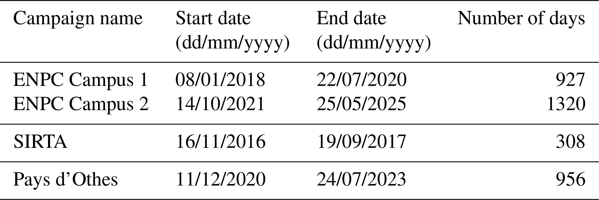
Figure 1 Location of the three measurement campaigns used in this paper. Coordinates system is WGS84 (EPSG:4326)

The first campaign, called ENPC-Campus, takes place on the roof of the Carnot building located on the campus of ENPC. In this paper, we use the rainfall data (only the rain rate in mm h⁻¹) measured with the help of a Parsivel² disdrometer manufactured by OTT, and temperature obtained with the help of a sensor by Campbell Scientific. Both devices provide data with 30 s time steps. The corresponding data base, references presenting the devices, description of the campaign, as well as complete samples of data can be found in Gires et al. (2018). The rainfall and temperature time series used in this paper for the second part of ENPC-Campus campaign are displayed in Fig. 2 as an illustration of the studied data in this paper.

From November 2016 to September 2017 the instruments were moved to SIRTA (Site Instrumenté de Recherche par Télédétection Atmosphérique) on the Ecole Polytechnique campus for a joint intensive measurement campaign over the Ile-de-France region, where Paris is located. The site is about 38 km away from ENPC campus towards south west of Paris. This campaign is denoted SIRTA in this paper, and is much shorter than the other two campaigns, meaning that the associated results are less robust.

The last measurement campaign used in this paper took place at a wind farm operated by Boralex and located at Pays d'Othe (name of the campaign), approximately 120 km south east of Paris in a slightly rolling area. As for the other campaigns, a Parsivel² disdrometer with 30 s time steps provided rainfall data. Temperature data were collected with the help of a mini meteorological station manufactured by Thies Clima and operated with a sampling rate of 1 Hz. Temperature data was upscaled to 30 s time steps to match the resolution of the rainfall data. The devices were installed on a meteorological mast at a height of 45 m. Complete description of the campaign and samples of data can be found in Gires et al. (2022).

The whole rainfall and temperature time series used in this paper, from each measurement campaign, can be accessed in Gires (2025).

Measurements of rainfall with the help of optical disdrometers are subject to instrumental limitations, notably calibration issues and influence of wind (see Lanza et al., 2021 for a review). Observed deviations can go up to roughly 10 % (Capozzi et al., 2021), and some correction scheme (when wind data is available) have recently been suggested (Chinchella et al., 2024, 2025). Addressing these issues and the influence of the associated uncertainty on the multifractal analysis carried out would be an interesting topic, but it remains outside the scope of this paper. Here, we can just mention that the portion of the rainfall time series with heaviest events are less affected by wind induced biases because they are associated with a greater portion of large drops which are less affected by these biases. Hence we expect a limited influence of these biases on UM analysis, which should be confirmed by dedicated analysis.

Figure 2 (Left) Time series of the rain rate during campaign “ENPC Campus 2”. (Right) Time series of the temperature during campaign “ENPC Campus 2”. 30 s time steps are used in both cases.

2.2 Sample selection at large scales

In a first step, analyses are carried out up to synoptic scale, which corresponds to the typical duration of a large scale meteorological situation with typical temporal extent of up to 10 d and spatial extent of up to 1000 km. This scaling regime is called “large scales” in the rest of the paper.

More precisely, for each measurement campaign, the whole time series of rain rate and temperature are split into successive samples of 2¹⁵ time steps, which corresponds to roughly 11.4 d. The process is initiated at the beginning of the available data without accounting for potential effects of diurnal variations. The paper focuses on rainfall, so potential snowfall should be removed in order to avoid introducing potential biases. In order to achieve this, all samples for which some “rainfall” was recorded while the temperature for the same time steps was below 4 °C were simply removed from the studied set of samples. Hail is very rare in these locations, and filters for potential hail were not implemented. The total number of samples per measurement campaign can be found in Table S1 of supplementary material. The total length of the studied samples corresponds to roughly 5.4, 0.7 and 2.0 years for the ENPC campus, SIRTA and Pays d'Othe measurement campaigns respectively.

2.3 Sample selection at event scale

Analyses were also implemented at event scale. To achieve this, rainfall events were selected by considering that a rainfall event is a rainy period of time during which more than 1 mm is collected and that is separated by more than 15 min of dry time steps before and after. More precisely, in order to identify them, a rainy time step found after a dry period of at least 15 min is considered as the start of a potential event. The end of the latter is the beginning of the next 15 min dry period. If the collected amount of rainfall is greater than 1 mm in between, then it is considered as a rainfall event. The number of events per measurement campaign can be found in Table S2 of supplementary material. As for the large scale analysis, events for which some “rainfall” was recorded while the temperature for the same time steps was below 4 °C were simply discarded (see supplementary material for numbers of events kept in analysis), in order to avoid potential biases associated with snowfall.

The selected rainfall events do not all have the same duration. Hence, a sample length is set for further joint analysis of the events. For technical reasons (see next section), it must correspond to a power of 2 of number of time steps. Longer sample lengths enable the study of rainfall across a wider range of scales, getting more robust results; but they impose to discard shorter events. Shorter sample lengths enable to keep a maximum of rainfall events; but limit the robustness of the results, being obtained across a more limited range of scales. As a trade-off, a sample length of 128 time steps corresponding to 64 min (∼ 1 h) was used. Then, in order to study the maximum possible data, the process illustrated in Fig. 3 was implemented for each event: (i) the maximum number of sub-events, i.e. non overlapping samples of size 128, was computed. It is equal to the integer part of the number of time steps of the event divided by 128 (ii) In order to study as much rainfall as possible, the portion of length equal to the product of the number of samples times 128 with highest cumulative depth was found within the time series of the event. Since disdrometer measurements were originally given at drop scale, there is a unique maximum. (iii) This selected portion was finally split into sample(s).

Figure 3 Illustration of how samples of 128 time steps (64 min) were extracted from a rainfall event that was collected during the ENPC-Campus campaign. In that case, three samples were extracted.

3 Methodology

3.1 Universal Multifractal framework

In this paper, variability and ultimately extremes of the rainfall times series across various ranges of scales, were quantified in the framework of Universal Multifractals (UM). Here, only the key elements are reminded and interested readers are referred to a recent review by Schertzer and Tchiguirinskaia (2020) and references therein for more details.

To introduce the framework, let us consider a conservative (i.e. its average does not change with scales) 1D time series ϵ_λ at a resolution λ. It is defined as the ratio between the outer scale (T_out) and observation scale (T_obs), i.e. $\mathit{\lambda }=T_{\mathrm{out}}/T_{\mathrm{obs}}$. For multifractal 1D time series, the moment of order q of the series exhibits a power law relation with regard to the resolution:

$$\begin{array}{}\text{(1)}& 〈{\mathit{ϵ}}_{\mathit{\lambda }}^q〉\approx {\mathit{\lambda }}^{K\left(q\right)}\end{array}$$

where K(q) is the scaling moment function. The notation 〈.〉 denotes the average over the time series. It can be shown that, in an equivalent way, the probability of exceeding a scale dependent threshold (λ^γ) defined with the help a scale-invariant singularity γ, also scales with the resolution as:

$$\begin{array}{}\text{(2)}& \mathrm{Pr}({\mathit{ϵ}}_{\mathit{\lambda }}\ge {\mathit{\lambda }}^{\mathit{\gamma }})\approx {\mathit{\lambda }}^{-c\left(\mathit{\gamma }\right)}\end{array}$$

where c(γ) is the codimension function (Schertzer and Lovejoy, 1987). The values of multifractal 1D time series behave as λ^γ. The singularity (γ) remains the same across scales while the value of the time series (λ^γ) changes with scales. The functions K(q) and c(γ) fully characterize the variability across scales of the time series ϵ_λ and are linked through a Legendre transform (Parisi and Frisch, 1985). This notably means that a singularity can be associated uniquely to each moment and vice-versa. Equations (1) and (2) also mean that multifractal properties are statistical properties which are valid on average over numerous samples.

In the specific framework of UM (Schertzer and Lovejoy, 1987), which are a limit behaviour of all multiplicative cascades processes (see discussion in Schertzer and Lovejoy (1997) for more details on this debates), K(q) and c(γ) are characterized with the help of only two parameters with physical interpretation:

• C₁, the mean intermittency co-dimension, which measures the clustering of the (average) intensity at smaller and smaller scales. C₁=0 for a homogeneous field;

• α, the multifractality index ($\mathrm{0}\le \mathit{\alpha }\le \mathrm{2}$), which measures the clustering variability with regard to the intensity level.

Greater values of α and C₁ correspond to stronger extremes. For UM, we have:

$$\begin{array}{}\text{(3)}& K\left(q\right)={\displaystyle \frac{C_{\mathrm{1}}}{\mathit{\alpha }-\mathrm{1}}}(q^{\mathit{\alpha }}-q).\end{array}$$

A Trace Moment (TM) analysis basically consists in checking the scaling behaviour of the time series and estimating K(q) by plotting Eq. (1) in log-log. To achieve this, the time series is upscaled from its maximum resolution Λ by averaging over adjacent time steps, then raised to various powers q, and finally the ensemble average (over various samples independently upscaled) is performed to obtain an estimate of the empirical moments and their scaling behaviour. UM parameters are estimated with the help of the Double Trace Moment technique which is an extension of TM tailored for UM (Lavallée et al., 1993).

Let us now consider a non-conservative 1D time series, denoted ϕ_λ, whose average changes with scales, i.e. we have 〈ϕ_λ〉≠1. In that case, it is usually assumed that it can be written as (with an equality in probability distribution):

$$\begin{array}{}\text{(4)}& {\mathit{\varphi }}_{\mathit{\lambda }}\stackrel{d}{=}{\mathit{ϵ}}_{\mathit{\lambda }}{\mathit{\lambda }}^{-H}\end{array}$$

where ϵ_λ is a conservative time series (〈ϵ_λ〉=1) of moment scaling function K_c(q) (the sub-index “c” refers to the conservativity of ϵ_λ), and H the non-conservation parameter. K_c(q) only depends on UM parameters C₁ and α. H characterizes the scale dependence of the average behaviour, and is equal to zero for a conservative time series. H should not be confused with the Hurst exponent: although both quantify long-range correlations for values greater than zero, the latter lacks a simple general expression for multifractal processes. It is notably not unique and needs to be generalized defining one for each studied statistical moment. H corresponds to the order of the fractional integration (if H>0) or differentiation (if H<0) needed to retrieve the studied process from a conservative one. More details about the link with the Hurst exponent can be found in Appendix A4 of Jose et al. (2024a), which is dedicated to this topic.

H is related to spectral analysis. Indeed, for scaling time series, the power spectrum follows a power law with regard to wave number:

$$\begin{array}{}\text{(5)}& E\left(k\right)\approx k^{-\mathit{\beta }}\end{array}$$

and the spectral slope β is related to H with the help of the following formula (Tessier et al., 1993):

$$\begin{array}{}\text{(6)}& \mathit{\beta }=\mathrm{1}+\mathrm{2}H-K_{\mathrm{c}}\left(\mathrm{2}\right)\end{array}$$

TM and DTM techniques should theoretically be implemented on a conservative time series ϵ_λ. However if H is roughly smaller than 0.3–0.4, it can be implemented directly on ϕ_λ, without substantially biasing the estimates of α and C₁. In case of greater H, ϵ_λ should be used in the TM and DTM techniques. Retrieving ϵ_λ from ϕ_λ theoretically requires a fractional integration of order H (equivalent to a multiplication by kH in the Fourier space). A common approximation, which provides reliable results, consists in taking ϵ_Λ as the absolute value of the fluctuations of ϕ_Λ at the maximum resolution and renormalizing it (Lavallée et al., 1993).

3.2 Maximum observable singularity

The insight one can get of a statistical process is limited by the size of the studied sample. For multifractal processes, this will result in a maximum singularity γ_s and corresponding moment order q_s beyond which the values of the statistical estimates of respectively the codimension and scaling moment functions are not considered as reliable (e.g., Lovejoy and Schertzer, 1989, 2007).

More precisely, let's consider N_s independent samples with a resolution λ. In a d-dimensional space, there are λ^d values per sample (d=1 for the time series studied in this paper). The maximum singularity (γ_s) that one can expect to observe in the available samples is defined by:

$$\begin{array}{}\text{(7)}& N_{\mathrm{s}}{\mathit{\lambda }}^d\mathrm{Pr}\left({\mathit{ϵ}}_{\mathit{\lambda }}\ge {\mathit{\lambda }}^{{\mathit{\gamma }}_{\mathrm{s}}}\right)\approx \mathrm{1}\end{array}$$

Introducing the notion of sampling dimension d_s: $N_{\mathrm{s}}={\mathit{\lambda }}^{d_{\mathrm{s}}}$ (d_S=0 for a single sample as it will be the case here), it yields:

$$\begin{array}{}\text{(8)}& c\left({\mathit{\gamma }}_{\mathrm{s}}\right)=d+d_{\mathrm{s}}\end{array}$$

which enables to estimate γ_s. For γ>γ_s one expects that $c\left(\mathit{\gamma }\right)=+\mathrm{\infty }$, which means that the estimates of c(γ) will not be reliable. As a consequence of the Legendre transform, the empirical estimates of K(q) become linear for $q>q_{\mathrm{s}}=c^{\prime }\left({\mathit{\gamma }}_{\mathrm{s}}\right)$: $K\left(q\right)={\mathit{\gamma }}_S(q-q_{\mathrm{s}})+K\left(q_{\mathrm{s}}\right)$. γ_s quantifies in a scale-invariant way the extremes that can be expected within a time series. The corresponding physical quantity at a given resolution λ is expressed as ${\mathit{\lambda }}^{{\mathit{\gamma }}_{\mathrm{s}}}$. It is especially useful to quantify how extremes evolve when α and C₁ exhibit different trends. Indeed, γ_s combines the influence of both UM parameters into a single one. For example, Royer et al. (2008) analysed rainfall output of climate models over France and found decreasing trend for α and increasing one for C₁. Relying on the notion of maximum observable singularity which combines the effects of both parameters, they showed that rainfall extremes are expected to increase over France in the context of climate change. Douglas and Barros (2003) used it to discuss the concept of maximum probable rainfall. Qiu et al. (2024) relied on this tool to quantify the impact of rainfall space-time variability on the usefulness of nature-based solutions in urban environment.

4 Results

4.1 Large scales

In this subsection, we implemented multifractal analyses on large scales, i.e. up to synoptic scale (see Sect. 2.2). In a first step, an ensemble analysis was carried out, that is to say all samples were upscaled independently and used to compute average statistical moments in Eq. (1) or spectra in Eq. (5). Such analysis is used to study general features of scaling.

Let us illustrate the results with the ENPC-Campus campaign. The outcome of spectral analysis, i.e. Eq. (5) in log-log, is displayed in Fig. 4a. A good scaling behaviour on scales ranging from roughly 30 min to 11 d is found, and smaller scales are investigated in next the subsection. The spectral slope β is smaller than 1, meaning that across this range of scales the studied time series is conservative and multifractal analysis can be implemented directly on the time series. Trace Moment analysis (i.e. Eq. 1 in log-log) outcome is displayed in Fig. 4b. The coefficients of determination of the linear regressions are all greater than 0.99 for q>0.5 and we use the one for q=1.5 as a metric. Results confirm the good scaling behaviour across this range of scales.

UM parameters estimated with the help of DTM technique are reported in Table 2. In the DTM technique, moments ranging from 1.3 to 1.7 (centered around the commonly used value of q=1.5) are tested enabling to provide an uncertainty range on the estimates of UM parameters. It corresponds to the uncertainty arising from the studied ensemble and not to the uncertainty arising from sample variability which is visible in the individual sample analysis below. The uncertainty on the DTM estimates of UM parameters tends to be larger when there are less samples. It remains in all cases smaller than 2.5 % and is very small compared to the differences between sites (and samples in upcoming analysis), so it will not be discussed further. UM parameters values are typical for this range of scales (e.g., Ladoy et al., 1993; de Lima and Grasman, 1999). The empirical scaling moment function K(q) derived from TM analysis and the theoretical one plotted using Eq. (3) and DTM estimates of UM parameters are in excellent agreement as it can be seen visually in Fig. 4.c. The discrepancies noticeable for q<0.5 are explained by a multifractal phase transition associated with the numerous zeros which are in the time series (see Gires et al. (2012) for more details on this phenomenon). Very small values of H (last column of Table 2), i.e. smaller than 0.1, corresponding to almost conservative time series, are retrieved for this range of scales.

Same good scaling behaviour was observed for this range of scales for the two other measurement campaigns. Similar UM parameters were retrieved with only limited variations of α and C₁ (see Table 2) according to the campaign.

Figure 4 For the campaign “ENPC campus” with ensemble analysis for large scales. (a) Spectral analysis, i.e. Eq. (5) in log-log. (b) TM analysis, i.e. Eq. (1) in log-log. (c) Scaling moment function K(q): empirical estimate and theoretically fitted shape using UM parameters from DTM analysis.

Table 2 Summary of UM parameters assessed across large scales (32 min – 11 d) using ensemble analysis for each measurement campaign

In a second step, in order to investigate how UM features are changing with temperature, the average temperature $<T>$ for each sample was computed from the available data. Even if the temperature also exhibits some variability, only the average temperature was considered. Joint multifractal analyses could be envisaged in future studies (e.g. Jose et al., 2024b). Then, two types of analyses were carried out:

• Individual sample analysis.

• Ensemble analysis of samples within a given range of temperature.

In the first type of analysis, a UM analysis was implemented on each sample individually using the same range of scales that was identified in the ensemble analysis. Individual samples with bad scaling, i.e. with r²<0.9 for q=1.5 were discarded (see supplementary material for numbers of samples kept in the analysis) from this analysis. Scaling being an average behaviour, it is expected that some samples do not exhibit a good scaling behaviour. And they were incorporated in the ensemble analysis before and the binned one after. Yet, adding their assessed parameters in the individual analysis would not be relevant because they are not reliable so they could bias results. Scatter plots of retrieved UM parameters vs. $<T>$ are displayed in Fig. 5 for ENPC-Campus campaign. Significant scattering is observed for all parameters. Potential overall trends were identified with the help of a linear regression, which corresponds to the simplest potential relationship. It is displayed through the red line on the plots. The quality of the linear regression was quantified with the help of the Pearson coefficient of correlation, denoted r. It ranges from −1 (exact linear relationship with negative slope) to 1 (exact linear relationship with positive slope). Values close to 0 correspond to lower levels of correlation. As a complement, Pearson p-value was computed in order to test the null hypothesis that the distribution of the underlying samples are uncorrelated. A threshold of 0.05 was used to reject the null hypothesis. In addition, Spearman rank correlation was also computed along with the corresponding p-value. Assessed slopes,Pearson coefficients of correlation r and Spearman rank correlation, along with associated levels of confidence are displayed in Table 3.

The $\left|r\right|$ coefficients are low, which is expected given the observed scattering. Similar comments can be drawn from the Spearman rank correlation. It means that the retrieved trends are only valid on average over numerous events, and they are not all statistically significant. For example, for H none of the observed trends for individual campaigns pass the statistical test of significance. Also, in the case of the SIRTA campaign, there are not enough samples to get statistically reliable trends. For the other two campaigns, we observed a decreasing trend for α and an increasing trend for C₁. Hence the consequences on extremes were not obvious and γ_s was needed to combine the effects of both. It appears that γ_s exhibits an increasing trend with $<T>$. It means that stronger variability and extremes are retrieved on studied samples with increasing temperature. A slightly decreasing trend is found for β and very slightly decreasing one for H. This suggests that at large scales, the long range correlation of the field tends to decrease with increasing temperature, i.e. that successive rainy periods are less correlated and more independent from one another.

Figure 5 For the campaign “ENPC campus” with individual sample analysis for large scales: r² for q=1.5 in TM analysis (a), α (b), C₁ (c), β (d), H (e) and γ_s (f) vs. $<T>$

Table 3 Slope ($\times {\mathrm{10}}^{-\mathrm{2}}$ °C⁻¹) (corresponding Pearson coefficient of correlation r, in bold if the null hypothesis of no trend was rejected; same for Spearman coefficient of correlation) of the linear regression of the value of the studied parameter vs. $<T>$ (individual sample analysis) at large scales. Illustration in Fig. 5 for “ENPC” Campus campaign.

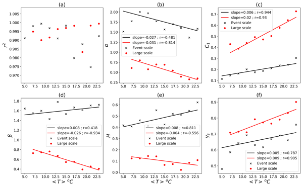
Keeping in mind that scaling is an average feature valid on numerous samples, a binned analysis was performed. It is not just the average values for all the events of a given bin that is considered, but the output of the ensemble analysis over all the samples of the bin. This enables to assess more robust scaling estimates which yields more reliable trends, even if some precision is lost with regard to temperature. More precisely, in the second type of analysis, the temperature range from 2 to 24 °C was split into bins of 2 °C width. Then, an ensemble analysis of all the samples whose average temperature is within a given bin was performed. Given that UM features from the various campaigns were very similar and in order to increase the number of samples to obtain more reliable results, all the available samples from all the campaigns were used. Results are displayed in Fig. 6 in red for the large scales studied in this subsection. First of all, the scaling (r²) is very good for all temperature bins. The total number of samples per bin is not the same (see Table S3 in Supplement), so a weighted linear regression (weights being the number of samples available) was performed to account for this. A larger data set would enable to explore whether this trend is real and associated with changes of precipitation type with temperature. The same trends that were obtained with the previous analysis are retrieved, i.e. α, β and H decrease with $<T>$, while C₁ and γ_s increase. The obtained trends exhibit much higher coefficients of correlation than in the previous analysis, as expected when aggregating across samples, though it does not independently strengthen the individual-sample evidence.

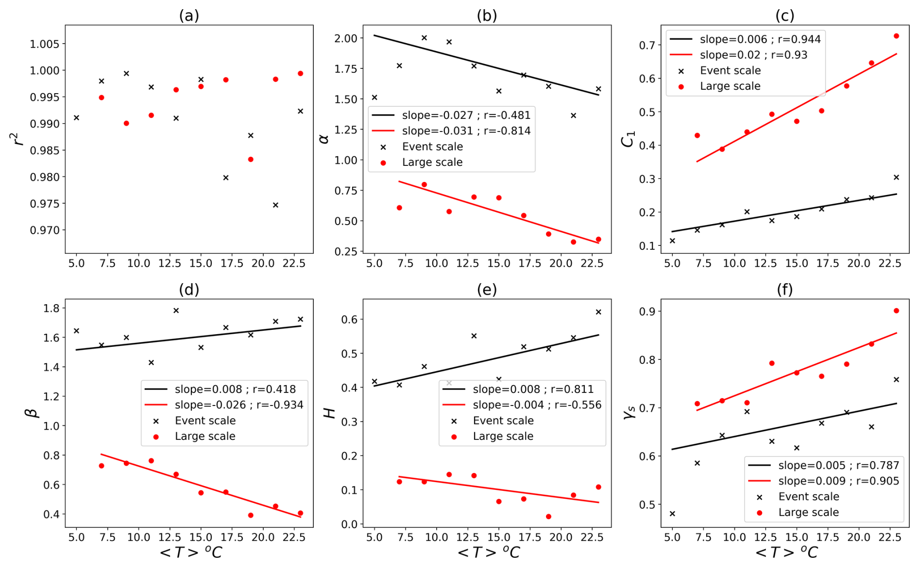
Figure 6 For all the campaign merged together and samples binned within classes of temperature of 2^oC width: r2 for q=1.5 in TM analysis (a), α (b), C₁ (c), β (d), H (e) and γ_s (f) vs. $<T>$

4.2 Event scale

In this subsection, analyses were carried out at event scale (see Sect. 2.3). The same analysis as for longer samples across large scales were carried out, with ensemble analysis first, to identify scaling behaviour, and then individual sample analysis in two formats.

Results are illustrated with the data from ENPC-Campus campaign. Spectral analysis (Fig. 7.a) shows that data exhibits a very good scaling behaviour on the whole range of scales from 30 s to 1 h. The spectral slope β is of 1.73 meaning that on this range of scales, the studied time series is not conservative, i.e. there are some strong long range correlations. Hence the analysis is done on the conservative part (see Sect. 3.1). Figure 7b shows TM analysis. The good scaling behaviour on the whole range of studied scales (30 s – 64 min) is confirmed, with coefficients of determination all greater than 0.99 for q>0.5.

UM parameters obtained via DTM analysis are in Table 4. These values, around 1.7–1.8 for α and 0.2 for C₁, are consistent with those commonly reported in the literature for this range of scales (e.g., Gires et al., 2016; de Montera et al., 2009; Mandapaka et al., 2009; Verrier et al., 2010; Jose et al., 2024b). Here we confirm them at even higher resolutions, which were not available in the previous studies. Similarly to the large scale analysis of previous section, the uncertainty on UM parameters estimates is very small compared to the differences observed between measurement campaigns and in between samples as we will see. Hence this will not be further accounted for. As for the results across large scales, there is a very good agreement between the empirical scaling moment function K(q) and the theoretical one. Some differences become visible for q greater than ≈2.3–2.5 which is slightly smaller than the expected value of q_s equal to 2.7 in this case.

Very similar qualitative and quantitative behaviour (see Table 4) were retrieved on this range of scales for the two other measurement campaigns.

Figure 7 For the campaign “ENPC campus” with ensemble analysis at event scale. (a) Spectral analysis, i.e. Eq. (5) in log-log. (b) TM analysis, i.e. Eq. (1) in log-log. (c) Scaling moment function K(q): empirical estimate and theoretically fitted shape using UM parameters from DTM analysis.

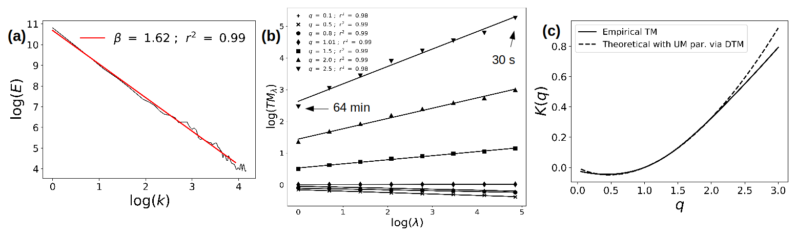
Table 4 Summary of UM parameters assessed at event scale (30 s – 64 min) using ensemble analysis

As for the large scales in the previous section, the average temperature $<T>$ over the whole event was assessed for each event, and the same two types of UM analyses on individual events (the sample(s) of a same event are analyzed together) and ensemble of events binned by temperature intervals were carried out.

As before and for the same reasons, the individual events with bad scaling, i.e. with r²<0.9 for q=1.5, were discarded (see supplementary material for numbers of samples kept in analysis). Scatter plots of retrieved UM parameters vs. $<T>$ are displayed in Fig. 8 for ENPC-Campus campaign. Stronger scattering than for the large scales is retrieved. Similarly potential overall trends were computed with the help of linear regressions. Slopes and r and p-value are reported in Table 5 for all measurement campaigns.

In general similar results but with less pronounced trends (smaller $\left|r\right|$) are retrieved for UM parameters with a slightly decreasing α, an increasing C₁ and an increasing γ_s. It means that variability and extremes also tend to increase with temperature over this range of scales. Contrarily to what is observed at large scales, β and H are increasing with temperature, corresponding to a greater non conservativeness of the time series. This suggests that with stronger temperature, the short range correlation within a given rainfall event tends to increase. It should be noted that opposing trends are observed for the dependency of H with regard to temperature for large scales (decreasing trend) and event scale (increasing trend). This suggests that warming is associated with greater within-event temporal coherence but reduced inter-event persistence, a finding that merits further investigation, to understand better which physical processes are involved in each case.

Table 5 Slope ($\times {\mathrm{10}}^{-\mathrm{2}}$ °C⁻¹) (corresponding Pearson coefficient of correlation r, in bold if the null hypothesis of no trend was rejected; same for Spearman coefficient of correlation) of the linear regression of the value of the studied parameter vs. $<T>$ (individual event analysis) at event scale. Illustration in Fig. 5 for “ENPC” Campus campaign.

Results for the binned analysis are displayed in Fig. 6 in black. As in the case of the large scales, they basically yield consistent trends with regard to the one discussed in the previous paragraph, with stronger correlations, as expected given the aggregation.

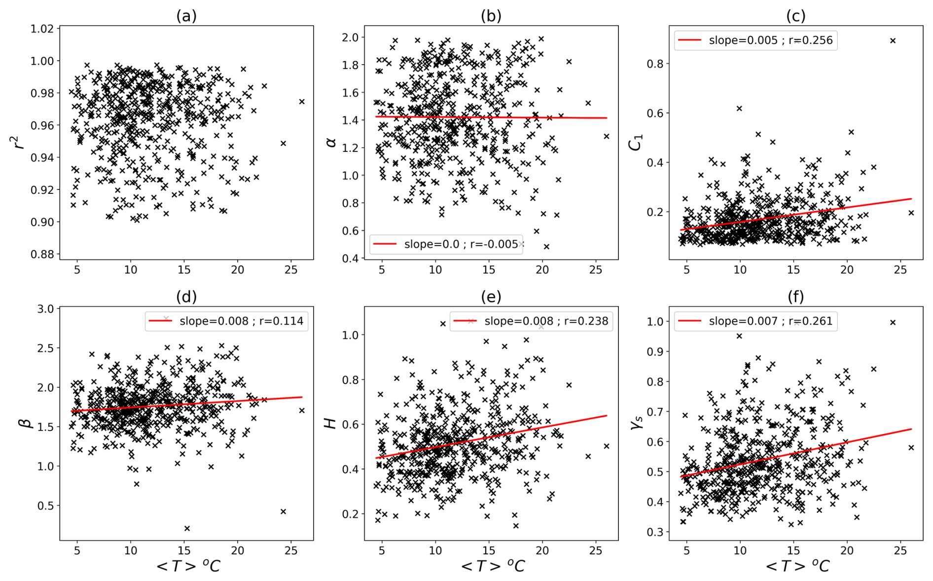
Figure 8 For the campaign “ENPC campus” with individual sample analysis at event scale: r² for q=1.5 in TM analysis (a), α (b), C₁ (c), β (d), H (e) and γ_s (f) vs. $<T>$

4.3 Seasonal and rainfall intensity sensitivity

Until now, all the analyses carried out account for events all around the year. In order to explore potential seasonal sensitivity, the same analysis was implemented considering the events for each season separately. The events/samples for which start month are December, January and February were labelled as winter. Similarly, the others were classified in spring (March, April, May), summer (June, July, August) and autumn (September, October, November). Slopes, as well as indicators of the quality of the linear regression of the value of the studied parameters vs. $<T>$ at both large and event scales for all measurement campaigns are displayed in Fig. 9. During winter, for large scales, $<T>$ for all samples ranged from 7.3 to 11 °C with an average value of 9.0 °C. Those numbers are equal to 8.5, 19 and 14 for spring, 17, 24 and 21 for summer and 6.9, 18 and 13 for autumn.

The “All” column corresponds to the results on average considering all the events of the whole years, which were discussed in the previous two sections. With regard to results according to seasons, it should first be mentioned that they are less statistically reliable, and this is notably due to the fact that the number of samples/events was lower (roughly divided by 4) than when all events were considered at once. Yet, it seems that some trends are visible. For example for γ_s at large scales, it appears that there is a slight decrease of it with increasing temperature (i.e. a negative slope is found), while the trend discussed in the previous subsection is valid for the other seasons. This could suggest that the temperature signal across all seasons on γ_s is partly affected by seasonal influence, i.e. that γ_s covaries with temperature associated regime shifts. This effect is less pronounced at event scale. β also seems to behave differently in winter for large scales (except for the SIRTA campaign for which there is a limited number of samples available). Longer time series would be needed to further confirm these preliminary observations.

Figure 9 Slope (°C⁻¹) of the linear regression of the value of the studied parameters vs. $<T>$ at both large and event scales for each measurement campaign for all events (left, it corresponds to values displayed in Tables 3 and 5) as well as per season. For each season, the 4 “columns” correspond in that order to all campaigns together, ENPC Campus, SIRTA and Pays d'Othe. Symbols are colored according to Pearson coefficient of correlation. The ones circled correspond to cases for which the null hypothesis of no trend was rejected.

In addition to these analyses, sensitivity to rainfall intensity and temperature were tested. More precisely, the same analysis considering only the events or samples with average rain rate belonging to the 10 % upper percentile was carried out. Using the available data, similar results were found, not enabling to detect some differences. An analysis splitting the events between those with average temperature below and above 12 °C also yielded similar results for both subset, not enabling to detect some differences. Studies on more events and other geographical areas would be needed to further investigate this, because other work found a dependency of the increase rate with temperature (e.g., Lenderink and van Meijgaard, 2008; Chagnaud et al., 2024) Indeed, some authors reported more pronounced trends when considering high or low temperature range or only the upper percentiles of rainfall extremes. Longer time series, enabling the study of more samples/events would be needed to implement this methodology to check whether similar effects are also found in this scale-invariant framework. Further analyses with longer time series and various climate types, would be interesting to carry out, to check for example how the extremes behave depending on rainfall types, i.e. stratiform vs. convective situations for example (e.g., O'Gorman, 2015).

4.4 Link with other studies

The analyses carried out did not aim at determining whether a super-CC or sub-CC is observed, since they focused on variability in general. Yet, given that rainfall extremes can be derived from some multifractal features, it is possible to relate the current results to previous findings available in the literature. More precisely, as discussed in the introduction, numerous studies have reported a scale dependence of the increase of rainfall extremes with temperature, i.e. that the increase is stronger in percentage for shorter durations (Fowler et al., 2021; Haerter et al., 2010; Lenderink and van Meijgaard, 2008; Lenderink et al., 2017; Panthou et al., 2014). Results presented here, provide a framework to interpret this.

In this study we find in general an increase of the scale invariant concept of maximum observable singularity γ_s of rainfall time series with temperature. γ_s being related to the extreme rainfall (greater γ_s corresponds to stronger extremes), one can note that, at least for small scales, it is consistent with previous findings from the literature reporting an increase of rainfall extremes with temperature. It is even possible to go a step further and explore how this increase is expected to change with observation scale. Indeed, the greater rainfall rate (i.e. an indicator of extreme rainfall) that one can expect to observe in a sample at resolution λ behaves as ${\mathit{\lambda }}^{{\mathit{\gamma }}_{\mathrm{s}}}$. We remind that λ is the resolution, i.e. the ratio between the outer scale and the observation scale, and that it increases with shorter duration. Hence, an increase of the scale invariant γ_s with temperature results in greater increase of extreme rainfall in percentage at higher resolutions, i.e. with shorter observation scales. Indeed, this percentage of increase %_incr can be written as:

$$\begin{array}{}\text{(9)}& {\mathit{\%}}_{\mathrm{incr}}=\mathrm{100}\times \left({\mathit{\lambda }}^{{\mathit{\gamma }}_{\mathrm{s}}\left(T_{\mathrm{1}}\right)-{\mathit{\gamma }}_{\mathrm{s}}\left(T_{\mathrm{2}}\right)}-\mathrm{1}\right)\end{array}$$

for a change from temperature T₁ to T₂. Hence the change with temperature in the scale invariant parameter γ_s provides a framework to explain changes in increase of rainfall extremes with temperature according to scale (mainly from daily to hourly) which were reported in previous studies. Indeed, with γ_s(T₁)−γ_s(T₂) fixed in Eq. (9) (i.e. the increase of γ_s with temperature), when λ increases (i.e. shorter durations are considered), the percentage of increase of the expected rainfall extreme rises. Let us consider an illustration with a temperature shift of 2 °C for the large scales. It corresponds to a shift of γ_s equal to 0.0077×2 (Table 3). T_out here is 11 d as shown in the multifractal analysis. At daily scale T_obs is one day. This yields to $\mathit{\lambda }=\mathrm{11}/\mathrm{1}$ which gives an increase of the maximum expected rainfall of roughly 4 %. At hourly scale T_obs is one hour, leading to $\mathit{\lambda }=\mathrm{11}/(\mathrm{1}/\mathrm{24})$ and an increase of roughly 9 % on expected maximum rainfall. This shows that relying on a scale invariant framework enables to grasp an understanding valid across a given range of observation scales. This constitutes a novelty with regard to previous studies. It should be mentioned that Emmanouil et al. (2022) found a faster strengthening of extremes for shorter duration with climate change using multifractal framework, which is a result consistent with what is reported here, using a different approach.

5 Conclusions

In this paper, we studied how rainfall extremes and more generally variability across scales changes with temperature. For this, we used data coming from three high resolution measurement campaigns that took place in France between 2018 and 2025; and we relied on the framework of Universal Multifractals. More precisely, we first confirmed scaling behaviour and then estimated UM parameters α, C₁, the corresponding maximum observable singularity γ_s, and H for each sample and studied their dependence on temperature. Such study, considering event and large scales, had not been done explicitly before.

It appeared that for scales ranging from 32 min up to the synoptic scale of roughly 11 d, a good scaling behaviour was retrieved and we observe in general a decrease of α with average temperature, an increase of C₁ which yields an overall increase of γ_s. There was a slight decrease of H. Retrieved trends are valid on average, with weak individual-sample/event correlations. Similar trends but less pronounced were observed at event scale, i.e. for scales ranging from 30 s to roughly 1 h, for α, C₁ and γ_s. On the contrary, an increasing trend with average temperature was found for H.

This increase of γ_s with temperature provides a scale-invariant observational complement to the existing multifractal-extremes literature on climate-forced rainfall changes. It also confirms previous findings of expected increase of rainfall extremes with temperature, which were not derived using scale invariant tools. Results also contribute to help explain the dependence of the rate of increase with the observation scale that is reported in previous studies.

Consistent results were found here between event and large scales and over three measurement campaigns. It suggests that findings are robust. Yet, the three stations used are located in a small meteorological region at planetary scale. It would definitely be relevant to expand the analysis to much wider areas using data from various climates to expand our understanding of the dependence of rainfall extremes with temperature. It would notably enable the exploration of temperature range greater than 23 °C which is the maximum available with the data set studied in this paper. Investigating the geographical dependence of the rate of change of UM parameters with temperature would notably be insightful and should be pursued in upcoming studies. It would also be very interesting to carry out similar analysis on the output of climate models, which are commonly used to investigate how rainfall extremes will change (e.g., Li et al., 2019; Dallan et al., 2024; Chagnaud et al., 2024). They notably enable gridded analysis to explore in detail longer time series as well as spatial patterns on the retrieved results, and could also help in overcoming issues like potential changes in the circulation regime. A major advantage of using model outputs is also the possibility to explore spatial extremes, i.e. how these results remain valid for various spatial scales, which is an important issue for hydrological impacts. Previous studies of rainfall in space-time suggest consistent results are expected, but this would need to be confirmed.

With regard to the potential impact of the work on the study of climate change, as for the other paper mentioned, the underlying idea is to first establish, when possible, a relationship between rainfall extremes and surface air temperature relying on data, and then to use temperature as a proxy to predict future rainfall extremes. Such reasoning relies on a strong assumption of stationarity in the physical processes generating rainfall, which may not be valid. This issue was not addressed in this work which focused on exploring the link between rainfall variability and extremes with temperature relying on current data, and should be investigated in future work.