Summertime evaporation over two lakes in the Schirmacher Oasis, East Antarctica

Amount of liquid water has been continuously grown in coastal Antarctica. It accumulated in the hydrological system including rivers and lakes existing both on ice surface and inside it. This complex hydrological system is poorly understood and it is challenging without comprehensive measurements of components of hydrological balance. This study focused on lake evaporation which were measured directly on two lakes located in the Schirmacher Oasis (70° S, Antarctica) with the eddy-covariance (EC) technique. The experiment lasted during two austral summers (December–February) in 2017–2018 and 2019–2020. The lakes were warmer than ambient air during whole summers, and they became ice free for the period of 3–6 weeks. The measurements showed that summertime evaporation varied from 0.3 to 5.0 mm d⁻¹, and depending on the ice cover presence, the average evaporation ranged from 1.5±0.1 mm d⁻¹ in December to 3.0±0.2 mm d⁻¹ in January–February. The EC measurements were used as a reference for evaluating uncertainties of five empirical formulas and bulk-aerodynamic method implementing various turbulent transfer coefficients. The bulk-aerodynamic method with locally adjusted turbulent transfer coefficients shows the most accurate estimates of daily rates of the lake evaporation (of 6 %–8 %). The empirical formulas underestimated the seasonal rate of lake evaporation by 27 %–73 %. Our results indicate that wind speed is the primary factor that controls summertime evaporation over the lakes. The largest day-to-day variations in evaporation were associated with changes in the wind speed.

1 Introduction

The Antarctic coast hosts numerous water bodies that store meltwater within a complex hydrological system of lakes and rivers. Every summer, approximately 60 000 surface lakes form on ice shelves (Corr et al., 2022; Dirscherl et al., 2021); the largest, reaching up to 80 km in length, are found in East Antarctica (Shen et al., 2025; Stokes et al., 2019). The presence of these water bodies accelerates the marginal calving of ice sheets – contributing to global sea level rise – and increases the risk of hydrofracturing-induced collapse of ice shelves (Rignot et al., 2004; Banwell et al., 2013). Large lakes also influence local weather: by providing a moisture source to the atmosphere through evaporation, they warm the air, increase precipitation, and foster fog formation (Blanken et al., 2003; Gultepe et al., 2003; Rouse et al., 2002; Gilson et al., 2018; Su et al., 2020).

Antarctica hosts approximately 120 permanent settlements, most of which are located along the continental coast, in rock oases, or on sub-Antarctic islands (COMNAP, 2017). These sites typically house between 20 and 80 people, primarily consisting of scientists, logistics personnel supporting fundamental research, and tourists. Antarctic tourism grew from about 6500 visitors in the 1991–1992 season to nearly 105 000 in the 2022–2023 season. Post-pandemic, arrival numbers of tourists increased by 40 % and are projected to grow by 12.5 % annually (Bastmeijer et al., 2023). Nearby lakes provide a crucial freshwater supply for the settlements; consequently, evaluating water resources is essential for managers planning site maintenance and infrastructure investments, as well as for mitigating hydrological risks (Lan et al., 2025). Assessing these resources requires reliable hydrometeorological observations and robust hydrological models. Furthermore, Antarctic lakes shelter unique life forms that are sensitive to human intrusion and climate change (Rothschild and Mancinelli, 2001; Andersen et al., 2011; Keskitalo et al., 2013). Understanding the hydrological regimes of these lakes is therefore vital for the conservation of these ecosystems (Faucher et al., 2019).

The lake water balance equation describes changes in lake volume as the difference between inflow components (e.g., surface/subsurface runoff, precipitation) and outflow components (e.g., evaporation/sublimation, artificial water withdrawal). Depending on the specific site and the integration timescale (e.g., daily, seasonal, decadal), the contribution of certain components may be negligible, while others remain essential. Evaporation, in particular, is a critical component of the water balance for lakes in polar regions (Li et al., 2016; Leppäranta et al., 2020; Wang et al., 2020; Shi et al., 2024). However, because evaporation is difficult to measure directly, it is often estimated using indirect methods that require only limited hydrological and meteorological observations (Morton, 1990; Finch and Hall, 2001; Spence et al., 2003).

A wide diversity of approaches exists to estimate lake evaporation indirectly from observations (Keijman, 1974; Spence and Hedstrom, 2015; Spank et al., 2025). These methods can be categorized into mass and energy balance models, bulk aerodynamic (mass-transfer) techniques, combination methods, equilibrium temperature models, empirical formulas, and the use of evaporation pans or tracers such as water isotopes (Finch and Hall, 2001; Finch and Calver, 2008; Abtew and Melesse, 2013; Bellagamba et al., 2021). The use of evaporation pans is a traditional approach that can provide high accuracy when properly calibrated (Stanhill, 2002). Alternatively, in mass and energy balance approaches, evaporation is typically estimated as the residual of the balance equation, provided all other components are known and accurately quantified (Singh and Xu, 1997; Stannard and Rosenberry, 1991; Abtew and Melesse, 2013).

The bulk-aerodynamic approach estimates evaporation based on data regarding land surface properties (type, temperature, and roughness) and atmospheric variables (wind speed, specific humidity, and air temperature) within the lowermost atmospheric boundary layer (Brutsaert, 1982). This method requires meteorological observations at different levels above the surface to calculate sensible and latent heat fluxes from their gradients. Evaporation is then derived by dividing the latent heat flux by the latent heat of vaporization. The bulk aerodynamic approach employs transfer coefficients for turbulence, heat, and moisture, which are derived from flux-gradient relationships and semi-empirical profiles for wind, temperature, and humidity (Yang and Bai, 2023). Under specific conditions, this method adequately estimates surface evaporation on daily or shorter timescales (Moore, 1983). This method has been widely applied to assess evaporation and sublimation over lakes and glaciers in Antarctica (Clow et al., 1988; Bliss et al., 2011; Leppäranta et al., 2016).

Combination approaches integrate elements of both the energy budget and mass-transfer principles (Penman, 1948). A more comprehensive form is the Penman-Monteith equation (Monteith, 1965), which was originally developed to estimate evapotranspiration from vegetated surfaces. In the empirical approach, daily or monthly lake evaporation rates are related to variables such as lake surface area, incoming solar radiation, diurnal minimum and maximum of air temperature and relative humidity (Konstantinov, 1968, Zhao et al., 2013, Spank et al., 2025). Simplified versions of both combination and empirical formulas have been applied to Antarctic lakes although their associated uncertainties are not well known (Borghini et al., 2013; Dhote et al., 2021; Kuznetsova et al., 2021). A key limitation of the empirical, mass transfer and combination approaches is that their performance is restricted to  the geographical and climatic conditions, under which their empirical coefficients were originally derived (Finch and Hall, 2001). To improve their applicability, the mass transfer coefficients are often calibrated based on measurements from eddy covariance (EC) systems (Ala-Könni et al., 2022; Nordbo et al., 2011). What is unknown is the actual range of values of the transfer coefficients for Antarctica, this study quantify them.

In this study, we evaluated summertime evaporation over two lakes in the Schirmacher Oasis (East Antarctica), using both the direct observations and various indirect mass-transfer methods. The study quantified the uncertainties of five empirical formulas and bulk-aerodynamic method by comparing them against eddy-covariance measurements collected during the austral summers of 2017–2018 and 2019–2020.

2 Study area

The Schirmacher Oasis (70°45^′ S, 11°38^′ E) is situated approximately 80 km from the coast of the Lazarev Sea, Dronning Maud Land (Fig. 1a). This oasis is an ice-free rock outcrop, approximately 20 km long and 3 km wide, elongated in a west-northwest to east-northeast direction (Simonov and Fedotov, 1964). The relief consists of rocky hills with elevations reaching up to 228 m above sea level (a.s.l.), primarily composed of gneiss mixed with basalt (Sengupta, 1991). Discovered in 1939, the site saw its first settlements emerge in the late 1960s. Today, the oasis hosts two year-round scientific observatories and two seasonally occupied tourist camps (Fig. 1b). The observatories are staffed by 15–25 overwintering personnel, with up to 30 additional staff visiting during the summer. The two tourist camps accommodate up to 20 people each and operate from November to February. Two ice runways support the transport of personnel and cargo; fuel and supplies are primarily delivered by ship to coastal bases on the ice shelf and subsequently transported to the settlements by vehicles. These settlements, ice runways, and coastal bases are connected by year-round ice roads (indicated by yellow lines in Fig. 1b). During the summer, transportation along these routes is often hindered by meltwater lakes and streams that form on the ice (Fig. 1c).

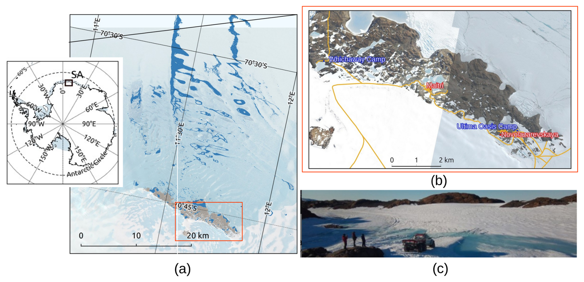
Figure 1 Location of the Schirmacher oasis (SA) (a) and its social infrastructure (b): year round (red dots) and seasonal (blue dots) settlements connected by roads (yellow lines, © Humanitarian OpenStreetMap Team (HOT), 2020. Distributed under the Open Data Commons Open Database License ((ODbL) v1.0.). In (a), the base map from © Google Earth 2025; images: © CNES/Airbus, Maxar Technologies, Airbus (21.12.201); the lake extent was taken from the cartographic layer from Stokes et al. (2019) (January 2017), and digitized from the map of scale 1:25 000 (published by the Ministry of Merchant Fleet of the USSR in 1969). The red boxes in (a) and (b) outline the area with the main infrastructure in SA, and the image (c) shows the a flooded section of the ice road leading to the Whichaway Camp (photo by Dmitrii Emelyanov, December 2019).

Lakes have existed in the Schirmacher Oasis since the Late Quaternary (Phartiyal et al., 2011), and today, the oasis is home to approximately 300 lakes (Gerrish et al., 2020). Most of these are freshwater bodies nourished by ice melt and seasonal snow cover, remaining ice-free for 6–12 weeks during the summer (Simonov, 1971). The largest lakes are glacial – directly attached to the ice sheet – and are often connected by temporary streams, forming chains that terminate in epishelf saline lakes (Loopman et al., 1988). Landlocked lakes, which have no connection to the ice sheet, are fed solely by snow melt and may evaporate over time, eventually forming hollows or dry beds (Fedorova et al., 2010). This study focuses on two glacial lakes that differ in volume and depth, both of which become ice-free for 2–8 weeks during almost every summer season (Khare et al., 2008; Sharov and Tolstikov, 2020).

Lake Zub (also known as Lake Priyadarshini) is the second-largest lake in the oasis, with a volume of 1.02×10⁶ m³. Its maximum depth is 6.0 m (mean depth: 2.9 m), and it has a surface area of 35×10³ m² (Dhote et al., 2021). During the 2017–2018 austral summer, the lake was ice-free from late December 2017 to early February 2018. Lake Zub/ Priyadarshini was reported to be thermally homogeneous during the period spanning from mid-January 1996 to mid-February 1997 (Sinha and Chatterjee, 2000). Lake Glubokoe is the deepest lake in the oasis, with a maximum depth of 34.5 m (mean depth: 13.1 m), a surface area of 147×10³ m², and a volume of 1.93×10⁶ m³ (Loopman et al., 1988). Until the late 1990s, it remained ice-covered year-round (Kaup, 2005).

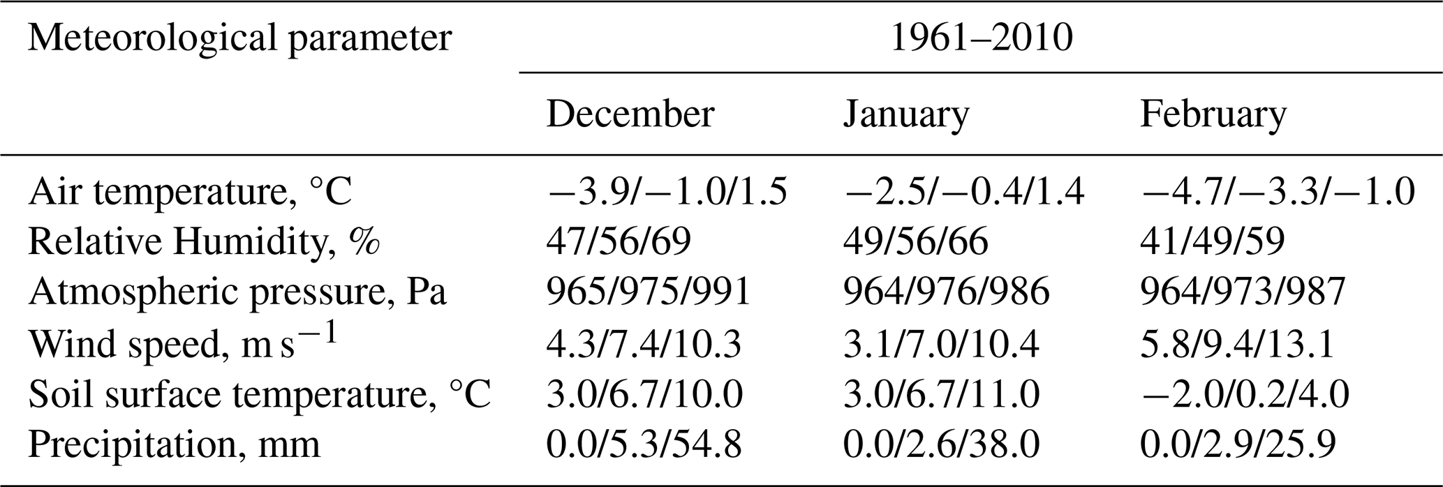
The climate of the Schirmacher Oasis is characterized by low air humidity and temperatures; persistent katabatic winds that occur throughout most of the year. Two scientific observatories operate within the oasis (Fig. 1a): the Novolazarevskaya (Novo) observatory (70°46^′36^′′ S, 11°49^′21^′′ E), which began observations in 1961, and the Maitri observatory (70°46^′00^′′ S, 11°43^′53^′′ E), which has been operational since 1989. These stations are situated approximately 5.5 km apart, and their meteorological measurements follow standards of the World Meteorological Organization (Turner and Pendlebury, 2004). Table 1 presents the monthly air temperature and relative humidity, averaged over the 1961–2010 period, based on observations from the Novo site (available at: http://www.aari.aq/default_ru.html, last access: 7 December 2021).

Table 1 The monthly minimum, mean and maximum values for the meteorological parameters calculated from the measurements for the period of 1961–2010 (the values are separated by a slash).

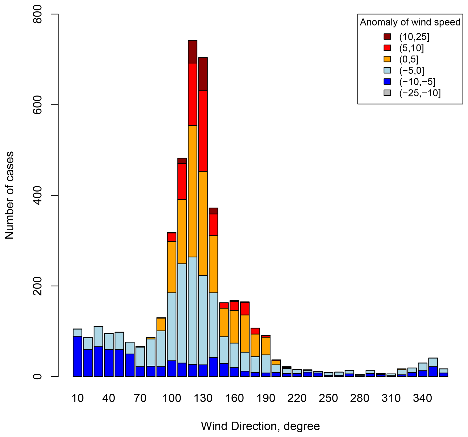
The study region is characterized by persistent katabatic winds blowing from the continental interior (Bormann and Fritzsche, 1995). To accurately capture eddy-flux measurements, it is essential to settle the instrumentation relative to the prevailing wind directions (Burba, 2013). Figure 2 illustrates wind directions and wind speed anomalies for December and January (1998–2016), calculated from 6-hourly synoptic observations at the Novo site, obtained from the British Antarctic Survey dataset (https://www.bas.ac.uk, last access: 14 December 2018). Prevailing winds range from 110 to 140° (indicated by black arrows in Fig. 2), consistent with the expected direction of katabatic flow. Wind speed anomalies were estimated for 10° directional bins and are represented by the colour-coded legend in Fig. 2. Positive wind speed anomalies are frequently observed within the prevailing wind range (indicated by orange, yellow, red, brown, and black colours in the legend); consequently, one can expect the majority of high-wind events to originate from these directions. However, the wind from the prevailing directions are not guaranteed to be of purely katabatic origin, as some may be driven by a combination of katabatic and synoptic forcing.

Figure 2 Wind direction and wind speed anomalies for December and January (1961–2010).

3 Data and methods

3.1 Micrometeological and hydrological observations

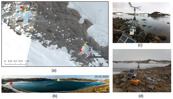
Measurements were collected on two lakes (Fig. 3a) across two separate field campaigns, covering 38 d in 2017–2018 and 33 d in 2019–2020. In the first experiment at Lake Zub /Priyadarshini, evaporation was measured while the lake was ice-free. The second experiment, conducted at Lake Glubokoe, captured the period of lake ice break-up. Although this experiment was originally designed to cover the entire austral summer, it was prematurely terminated in mid-January due to instrumentation failure.

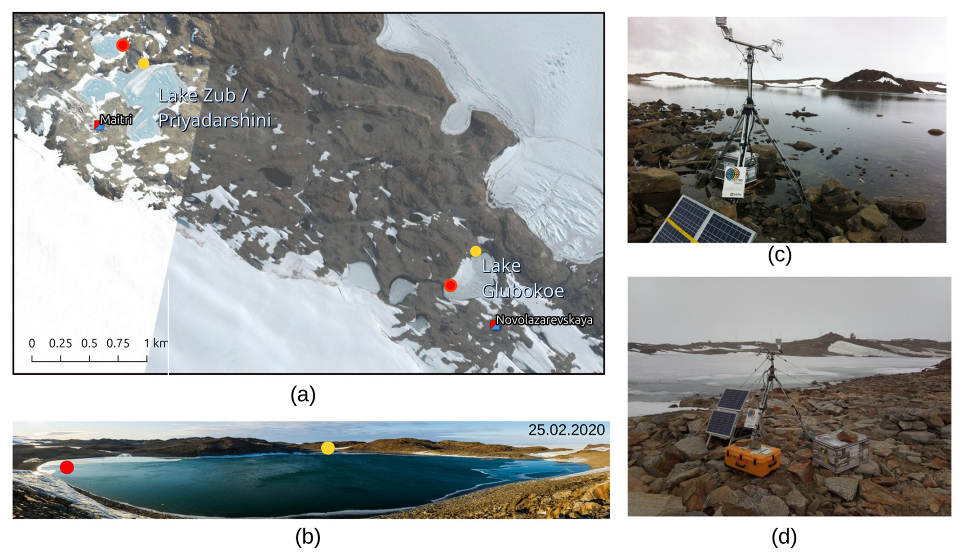
Figure 3 Location of the instrumentation on the shores of two lakes (a): temperature and water level logger (red dots), the EC system (yellow dots). In (a) the base map from © Google Earth 2025; images: © CNES/Airbus, Maxar Technologies, Airbus (21.12.201); the location of research observatories was taken from Quantarctica (Matsuoka et al., 2018). The photo (b) shows the location of the instrumentations installed on Lake Glubokoe (25 February 2020). The photos on (c) and (d) show the EC system installed on the shore of Lake Zub/Priyadarshini (6 January 2018) and Lake Glubokoe (12 December 2019).

Air temperature, atmospheric pressure, wind speed and direction, water vapor concentration and relative humidity were measured using an IRGASON open-path EC system (Campbell Scientific). The instrument integrates a 3D sonic anemometer and gas analyser that measure ${\mathrm{CO}}_{\mathrm{2}}/{\mathrm{H}}_{\mathrm{2}}\mathrm{O}$ concentrations on a high frequency (10 Hz). The system was positioned 5–6 m from the lake shoreline and oriented toward the lake to align with prevailing wind directions. Lake surface water temperature (LSWT) was measured using HOBO sensors (indicated by red dots in Fig. 3a) installed at a depth of 0.2 m. Prior to installation, we conducted a 1–2 d inter-calibration of our sensors against the sensors installed at Novo observatory (data not shown).

3.2 Methods

3.2.1 Eddy-covariance measurements

The eddy-covariance (EC) technique was used to measure evaporation from the two study lakes. Raw measurements were processed with the EasyFlux software provided by the instrument manufacturer, and then post-processed following the method described by Potes et al. (2017). We also included screening to remove spikes (Vickers and Mahrt, 1997); the frequency of these spikes was recorded for quality control purposes. Although the EC instrumentation collects gas concentration data across the full 0–360° range, only data associated with the footprint over the lake surface were utilized. These measurements were filtered using the footprint model defined by Kljun et al. (2004). The quality-controlled and filtered measurements cover more than 80 % of raw data. Furthermore, air relative humidity and the saturation vapour pressure deficit – defined as the difference between air and water temperatures – were calculated following Hoeltgebaum et al. (2020) and Stull (2017), respectively.

3.2.2 Empirical formulas

The general form of the formulas reads as $E=K{w}_z\left(e_{s-}{e}_z\right)$, where E is the evaporation (mm per period), w_z is the wind speed (m s⁻¹), (e_s−e_z) is the water vapour deficit (kPa), z refers to height (m), and K is an empirical function approximated with a small number of coefficients. In this study, we evaluated evaporation over two lakes with the formulas originally derived for tropical, temperate and cold climate regions (Table 2).

Table 2 The empirical equations applied to evaluate the lake evaporation.

In these formulas, E is evaporation (mm d⁻¹), w₂ is the wind speed at 2 m height (m s⁻¹), and A is a lake surface area (m²). We also verified against the independent observations the formula $E=-\mathrm{0.33}(\mathrm{1}-\mathrm{1.82}{w}_{\mathrm{2}})(e_s-e_{\mathrm{2}})$ suggested in Shevnina et al. (2022).

3.2.3 Bulk-aerodynamic method

Evaporation is defined as the vertical surface flux of water vapour due to atmospheric turbulent transport. Lake evaporation is estimated from measurements of a lake water surface temperature, and relevant bulk properties of the air (Brutsaert, 1982). We calculated the evaporation (kg m⁻² s⁻¹) after the bulk-aerodynamic methods as follows:

$$\begin{array}{}\text{(1)}& E=\mathit{\rho }{C}_{\mathrm{E}z}\left(q_{\mathrm{s}}-q_{az}\right)w_z\end{array}$$

where, ρ is the air density (kg m³); C_E is the turbulent transfer coefficient for moisture (Dalton number) at height z; q_s is the saturation specific humidity corresponding to the lake surface water temperature, q_az is the air specific humidity at height z, and w_z is the wind speed at height z. The turbulent transfer coefficient (C_Ez) depends on surface roughness and atmospheric stability, which we determined using both field measurements (eddy covariance and gradient) and values reported in the literature. For literature-based estimates, we utilized a value of C_E=0.00107, as suggested by Heikinheimo et al. (1999) for boreal lakes. This value allows for a more accurate representation of the turbulent mixing regime over small lakes compared to marine environments (Sahlée et al., 2014).

Since the atmospheric surface-layer is not always neutral, the stability effects on the turbulent transfer coefficient C_EZ were taken into account as follows:

$$\begin{array}{}\text{(2)}& C_{\mathrm{E}z}={\displaystyle \frac{C_{\mathrm{D}zN}^{\mathrm{1}/\mathrm{2}}{C}_{\mathrm{E}zN}^{\mathrm{1}/\mathrm{2}}}{\left[\mathrm{1}-\left(\frac{C_{\mathrm{D}zN}^{\mathrm{1}/\mathrm{2}}}{k}\right){\mathit{\psi }}_m\left(\frac{z}{L}\right)\right]\left[\mathrm{1}-\left(\frac{C_{\mathrm{E}zN}^{\mathrm{1}/\mathrm{2}}}{k}{\mathit{\psi }}_q\left(\frac{z}{L}\right)\right)\right]}}\end{array}$$

where C_DzN is the drag coefficient for a lake surface (unitless), k is the von Karman constant (0.4), ψ_m and ψ_q are the stability functions for momentum and moisture, respectively, and L is the Obukhov length (metre) (Obukhov, 1946). The subscript N in Eq. (2) refers to the neutral values of the transfer coefficients. The Obukhov length was used to adjust the transfer coefficients (C_D and C_E) to account for atmospheric stability in the surface layer. For our calculations, the value of drag coefficient (C_DzN) was set to 0.00181, following Heikinheimo et al. (1999). As these values were originally referenced to z=3 m, we adjusted them to our observation heights (z=2 m and z=1.8 m) using the approach proposed by Launiainen and Vihma (1990). This same algorithm was applied to iteratively solve the interdependency between turbulent fluxes and the Obukhov length. Stability functions were defined using the classic formulation by Businger et al. (1971) for unstable stratification and by Holtslag and De Bruin (1988) for stable stratification. Furthermore, the turbulent transfer coefficient (C_E) and the drag coefficient (C_D) were adjusted from the EC measurements. Specifically, a wind-dependent  C_E was derived from EC measurements at Lake Zub/Priyadarshini during the 2017–2018 season and subsequently applied to calculate evaporation using Eq. (1) for independent observations collected at Lake Glubokoe (2019–2020).

The drag coefficient (C_Dz) and the moisture transfer coefficient (C_Ez) were also estimated based on EC measurements from Lake Glubokoe (2019–2020) and subsequently applied to calculate evaporation from observations at Lake Zub/Priyadarshini (2017–2018). Following Arya (1988), the coefficients were calculated as follows:

$$\begin{array}{}\text{(3)}& {\displaystyle }{C}_{\mathrm{D}z}={\displaystyle \frac{k^{\mathrm{2}}}{{\left[\ln \left(\frac{z}{z_{\mathrm{0}\mathrm{m}}}\right)\cdot {\mathrm{\Psi }}_m\left(\frac{z}{L}\right)\right]}^{\mathrm{2}}}}.\text{(4)}& {\displaystyle }{C}_{\mathrm{E}z}={\displaystyle \frac{k^{\mathrm{2}}}{\left[\ln \left(\frac{z}{z_{\mathrm{0}\mathrm{m}}}\right)\cdot {\mathrm{\Psi }}_m\left(\frac{z}{L}\right)\right]\cdot \left[\ln \left(\frac{z}{z_{\mathrm{0}q}}\right)\cdot {\mathrm{\Psi }}_q\left(\frac{z}{L}\right)\right]}}.\end{array}$$

where z_0 m is the momentum roughness length (metre) and z_0q is the roughness length for water vapour (metre), according Fedorovich et al. (1991):

$$\begin{array}{}\text{(5)}& {\displaystyle }{z}_{\mathrm{0}\mathrm{m}}={\displaystyle \frac{\mathrm{0.135}{\mathit{\nu }}_a}{u_{\ast }}};u_{\ast }\le \mathrm{10.856}\left(\mathrm{cm}{\mathrm{s}}^{-\mathrm{1}}\right),\text{(6)}& {\displaystyle }{z}_{\mathrm{0}\mathrm{m}}={\displaystyle \frac{u_{\ast }^{\mathrm{2}}}{\mathrm{69}g}};u_{\ast }>\mathrm{10.856}\left(\mathrm{cm}{\mathrm{s}}^{-\mathrm{1}}\right),\text{(7)}& {\displaystyle }{z}_{\mathrm{0}q}={\displaystyle \frac{\mathrm{9.072}\times {\mathrm{10}}^{-\mathrm{2}}}{u_{\ast }}};u_{\ast }\le \mathrm{10.856}\left(\mathrm{cm}{\mathrm{s}}^{-\mathrm{1}}\right),\text{(8)}& {\displaystyle }\begin{array}{rl}& z_{\mathrm{0}q}=\mathrm{8.357}\times {\mathrm{10}}^{-\mathrm{3}}-\mathrm{1.904}\times {\mathrm{10}}^{-\mathrm{4}}\left(u_{\ast }-\mathrm{10.856}\right);\\ & \mathrm{10.856}<u_{\ast }<\mathrm{22.622}\left(\mathrm{cm}{\mathrm{s}}^{-\mathrm{1}}\right),\end{array}\text{(9)}& {\displaystyle }\begin{array}{rl}& z_{\mathrm{0}q}=\mathrm{1.092}\times {\mathrm{10}}^{-\mathrm{4}}{u}_{\ast }^{\mathrm{2}}{e}^{-\mathrm{0.228}{u}_{\ast }^{\mathrm{3}/\mathrm{4}}};\\ & u_{\ast }>\mathrm{10.856}\left(\mathrm{cm}{\mathrm{s}}^{-\mathrm{1}}\right).\end{array}\end{array}$$

where u_∗ is the friction velocity (m s⁻¹). The stability functions ψ_m and ψ_q assume the following forms:

$$\begin{array}{}\text{(10)}& {\displaystyle }\begin{array}{rl}& {\mathrm{\Psi }}_m\left({\displaystyle \frac{z}{L}}\right)=\ln \left[\left({\displaystyle \frac{\mathrm{1}+x^{\mathrm{2}}}{\mathrm{2}}}\right){\left({\displaystyle \frac{\mathrm{1}+x}{\mathrm{2}}}\right)}^{\mathrm{2}}\right]-\mathrm{2}{\tan }^{-\mathrm{1}}x+{\displaystyle \frac{\mathit{\pi }}{\mathrm{2}}}\\ & \text{for }\left({\displaystyle \frac{z}{L}}<\mathrm{0}\right),\end{array}\text{(11)}& {\displaystyle }{\mathrm{\Psi }}_q\left({\displaystyle \frac{z}{L}}\right)=\mathrm{2}\ln \left({\displaystyle \frac{\mathrm{1}+x^{\mathrm{2}}}{\mathrm{2}}}\right)\text{ for }\left({\displaystyle \frac{z}{L}}<\mathrm{0}\right),\text{(12)}& {\displaystyle }{\mathrm{\Psi }}_m\left({\displaystyle \frac{z}{L}}\right)={\mathrm{\Psi }}_q\left({\displaystyle \frac{z}{L}}\right)=-\mathrm{5}\left({\displaystyle \frac{z}{L}}\right)\text{ for }\left({\displaystyle \frac{z}{L}}\ge \mathrm{0}\right),\end{array}$$

where $x={\left[\mathrm{1}-\mathrm{16}\left(\frac{z}{L}\right)\right]}^{\frac{\mathrm{1}}{\mathrm{4}}}$. The value of the transfer coefficient of moisture (C_E) was further referred to Arya (1988).

Also, we also estimated the transfer coefficient of moisture as suggested in Andreas (1986):

$$\begin{array}{}\text{(13)}& {\displaystyle }{C}_{\mathrm{D}z}={\displaystyle \frac{k^{\mathrm{2}}}{\ln \left(r/z_{\mathrm{0}}\right)}},\text{(14)}& {\displaystyle }{C}_{\mathrm{E}z}={\displaystyle \frac{{\mathit{\alpha }}_{E}k{C}_{\mathrm{D}z}^{\mathrm{1}/\mathrm{2}}}{k{C}_{\mathrm{D}z}^{-\mathrm{1}/\mathrm{2}}-\ln \left(z_Q/z_{\mathrm{0}}\right)}},\end{array}$$

where, the values of the z_Q and z₀ were taken as the functions of the roughness Reynolds number, and were depended on the wind speed and on the surface roughness parameter; r is a reference heigh (10 m); and α_E=1.

The estimated uncertainties of the indirect methods rely on the eddy-covariance (EC) technique (Shi et al., 2024). To evaluate the skill of the indirect methods we apply the root mean square error $(\text{RMSE}=\sqrt{{\sum }_{\mathrm{1}}^n{\left(E_{\mathrm{EC}}-E_{\mathrm{mod}}\right)}^{\mathrm{2}}})$ following Moriasi et al. (2007). To define if a method is acceptable to be used in hydrological practice or not, we applied the $s/\mathit{\sigma }$ criteria following to Popov (1979). In $s/\mathit{\sigma }$ criteria, $s=\sqrt{{\sum }_{i=\mathrm{1}}^n{\left(E_{\mathrm{EC}}^i-E_{\mathrm{mod}}^i\right)}^{\mathrm{2}}/\left(n-m\right)}$ and $\mathit{\sigma }=\sqrt{{\sum }_{i=\mathrm{1}}^n{\left(E_{\mathrm{EC}}^i-{\stackrel{\mathrm{‾}}{E}}_{\mathrm{EC}}\right)}^{\mathrm{2}}/n}$ where, E_EC is the evaporation by the eddy covariance method, E_mod is evaporation by an indirect method; $\stackrel{\mathrm{‾}}{E}$ is the mean evaporation, (mm d⁻¹); n is the length of the series, and m is the number of empirical coefficients in the relationships (equal to 2 in our case). The mean daily evaporation over the observational period and its error (${\mathit{\sigma }}_{\stackrel{\mathrm{‾}}{E}}=\frac{\mathit{\sigma }}{\sqrt{n}}$) were calculated following Rozhdestvensky and Chebotarev (1974).

4 Results

4.1 Weather conditions and lake surface water temperature

During the 2017–2018, daily mean air temperatures ranged from −5.6 and 2.4 °C, while daily mean wind speeds varied between 1.3 and 13.2 m s⁻¹. Throughout January and February 2018, the mean daily wind speed was 6.3 m s⁻¹, and the mean daily relative humidity was 54 % (ranging from 39 % to 77 %). Relative humidity reached 90 % and more on 3 January and 2 December 2018. In 2019–2020, daily mean air temperature ranged from −1.4 to 2.6 °C, with an average of 1.0 °C. The daily mean of the air temperature fluctuations spanned −4.9 and 5.1 °C, and warmest days were observed in late December 2019. Mean mean humidity was 56 % (varying between 43 % and 77 %), with daily maximums exceeding 90 % on 25–26 December 2019. Mean daily wind speed ranged from 1.3 to 9.5 m s⁻¹, averaging 5.9 m s⁻¹ across the experiment period. The strongest wind events (speed reached 13.0 m s⁻¹) were observed on 8 December 2019 and 1 January 2020, and the weakest wind events (speed below 0.5 m s⁻¹) occurred on 21–25 December 2019 and 3 January 2020.

Throughout the experimental periods, both Lake Zub/Priyadarshini and Lake Glubokoe were warmer than the ambient air. Between 30 December 2017 and 9 February 2018, the mean daily LSWT at Lake Zub/Priyadarshini was 3.9 °C, which was 4.7 °C higher than the mean air temperature (Fig. 4a). The temperature difference between the lake surface and the air varied from −0.5 °C (2–3 January 2018) to 10.0 °C (25–26 January 2018). Similarly, from 7 December 2019 to 15 February 2020, the mean daily LSWT at Lake Glubokoe was 3.1 °C (ranging from 0.6 to 5.3 °C); on average, the lake was 2.4 °C warmer than the ambient air during this period (Fig. 4b). The largest temperature gradient between the LSWT and the air was observed on 25–26 December 2019.

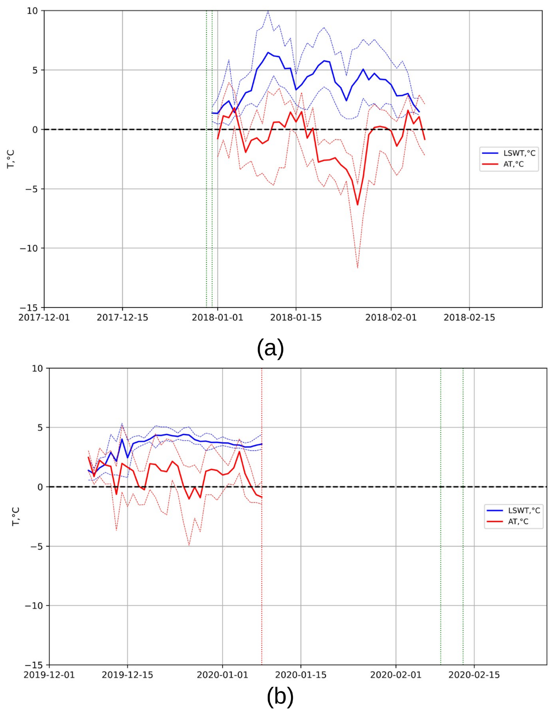
Figure 4 Daily minimum, mean and maximum for the air temperature (red lines) and LSWT (blue lines) measured during the experiments on Lake Zub/Priyadarshini (a) and Lake Glubokoe (b). In (b) the red line shows 8 January 2020. The green lines in (a) and (b) show the days when the lakes became free of ice.

4.2 Eddy-covariance

Direct measurements of evaporation were a key component of this study. The open-path EC system was installed on a location allowing it to cover the lake surface sector which was between 105 and 240° for Lake Zub/Priyadarshini, and between 90 and 225° for Lake Glubokoe (green lines on Fig. 5). Figure 5a and b show radial histograms (bar chars given around a circle) for the two experiments, where the height of the bars represents the frequency (number of cases) and the colour segments within each bar represent the mean wind speed. During the Lake Zub/Priyadarshini experiment, and in the most frequent sector the mean wind speed was of 6.5 m s⁻¹. At Lake Glubokoe, a maximum wind speed of 5.5 m s⁻¹ observed in the most frequent sector of wind directions. In Fig. 5c and d, the radial histograms show the XR90 (m) representing the horizontal distance over the lake surface that encompasses 90 % of the flux footprint. During the Lake Zub/Priyadarshini experiment, mean XR90 ranged from 95 to 135 m, and in the most frequent sector it was approximately 120 m. For the Lake Glubokoe, the mean XR90 ranged from 70 to 190 m, with a value of approximately 90 m in the most frequent sector.

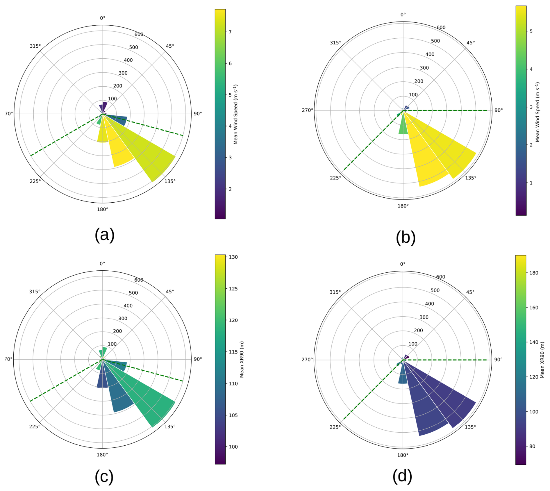
Figure 5 The wind speed and direction measured at IRGASON site (a: Lake Zub/Priyadarshini, and b: Lake Glubokoe) and the footprint length estimate (XR₉₀, m) (c: Lake Zub/Priyadarshini, and d: Lake Glubokoe). The green lines indicate the footprint sector.

The installation height of the IRGASON system (1.8–2 m) creates a “blind zone” surrounding the instrument, ensuring that the shoreline and its surrounding terrain do not interfere with the flux measurements. Furthermore, this low installation height ensures that the vertical divergence of the water vapour flux remains negligible. The raw 30 min measurements were filtered based on the sensor signal strengths, data gaps, footprint modelling and the specific wind direction sectors covering the lake. Less than 20 % of the total data were excluded; the majority of these exclusions resulted from wind directions originating outside the lake sector. These gaps were replaced by mean evaporation estimated for the experimental period. Hourly, daily and seasonal cumulative sum were further calculated from the filled data. Figure 6 illustrate the filtered evaporation that were excluded from analysing in the experiment on Lake Glubokoe (2019–2020) where red lines delineate sector of wind directions covering the lake surface (a) and the red dots represent the filtered data points (b).

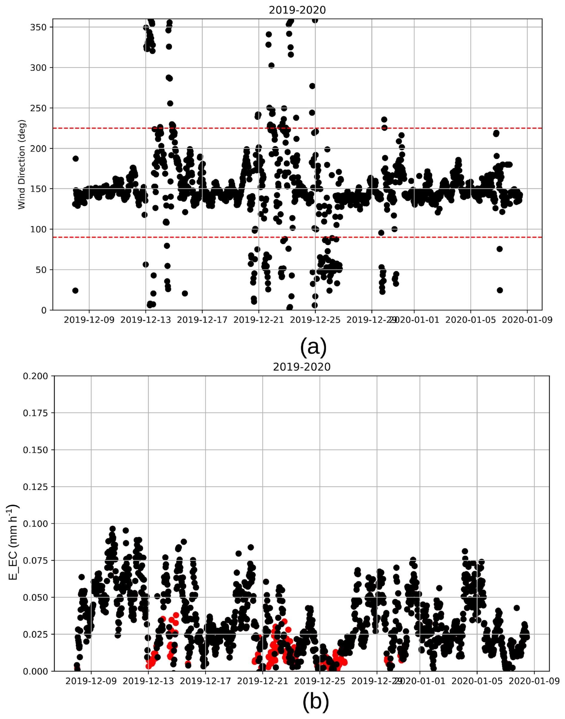
Figure 6 The 30 min means of the wind direction (a) and evaporation (b) measured by the EC instrumentation on Lake Glubokoe. On (a), the red lines show the limit of the wind directions within the footprint; on (b), the red dots indicate the measurements collected outside the foot.

For Lake Zub/Priyadarshini, daily mean evaporation rate varied from 1.5 to 5.0 mm d⁻¹ with an average of 3.0±0.3 mm d⁻¹. This average was derived by dividing the total evaporated water (114 mm) by the duration of the experiment (38 d). Evaporation rates increased with wind speed, peaking at 5.0 mm d⁻¹ during the storm event on 2–3 January 2018. For Lake Glubokoe, the daily mean evaporation rate varied between 0.3 and 3.2 mm d⁻¹, averaging 1.5±0.1 mm d⁻¹ with a cumulative total of 54 mm over the experimental period. The highest evaporation rates (>2.5 mm d⁻¹) occurred on 9–11 December 2019 and 3–4 January 2020, while the lowest rates (<0.9 mm d⁻¹) were observed on 6–7 January 2020.

4.3 Empirical formulas

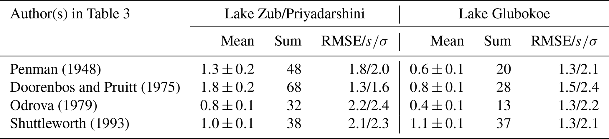
Evaporation was estimated using four empirical formulas: the resulting mean daily evaporation rates ranged from 0.4±0.1 to 1.1±0.1 mm d⁻¹, representing values 27 %–73 % lower than those derived from the eddy covariance method  (Table 3). The formula proposed by Shevnina et al. (2022) yielded a daily mean evaporation rate of 1.5±0.2 mm d⁻¹ for the ice-covered Lake Glubokoe (based on independent data), which is only 6 % lower than the rate calculated via the EC technique. Overall, the performance of these formulas was suboptimal: the ratio of the standard deviation of the error (s) to the standard deviation of the observations (σ) was $s/\mathit{\sigma }>\mathrm{2}$, and the root-mean-square error (RMSE) reached 2.2 mm d⁻¹.

Table 3 The evaporation over two glacial lakes on the basis of the empirical formulas and their skill scores. The daily mean evaporation in mm d⁻¹ , and the cumulative sum is given in mm per period.

4.4 Bulk-aerodynamic method

We estimated the lake evaporation on the basis of the observed wind speed, lake surface temperature, and air specific humidity, applying three literature based formulae for C_EzN (Heikinheimo et al., 1999; Arya, 1988; Andreas, 1986). In addition, the actual values of the transfer coefficient were derived from the direct observations on evaporation, wind speed, air specific humidity, and surface saturation specific humidity collected during the experiment on Lake Zub/Priyadarshini (2017–2018). Using Eq. (1), 30 min mean values of C_E2 were solved on the basis of the observed evaporation, q_s, q₂ and w₂. Finally, to facilitate comparison with literature-based relationships for the standard height of 10 m, we converted the C_E2N values to C_E10N applying the iterative algorithm of Launiainen and Vihma (1990). The result demonstrated an approximately piecewise linear relationship between w₂ and C_EzN (Fig. 7). Linear regressions were derived for the wind regimes below and above 13 m s⁻¹, separately for C_E10N and C_E2N as follows:

$$\begin{array}{}\text{(15)}& {\displaystyle }{C}_{\mathrm{E}\mathrm{10}N}=\mathrm{0.0000119}{w}_{\mathrm{2}}+\mathrm{0.00114}\text{ if }{w}_{\mathrm{2}}<\mathrm{13}\mathrm{m}{\mathrm{s}}^{-\mathrm{1}},\text{(16)}& {\displaystyle }{C}_{\mathrm{E}\mathrm{10}N}=\mathrm{0.0013}\text{ if }{w}_{\mathrm{2}}>\mathrm{13}\mathrm{m}{\mathrm{s}}^{-\mathrm{1}}.\text{(17)}& {\displaystyle }{C}_{\mathrm{E}\mathrm{2}N}=\mathrm{0.0000193}{w}_{\mathrm{2}}+\mathrm{0.00153}\text{ if }{w}_{\mathrm{2}}<\mathrm{13}\mathrm{m}{\mathrm{s}}^{-\mathrm{1}},\text{(18)}& {\displaystyle }{C}_{\mathrm{E}\mathrm{2}N}=\mathrm{0.0018}\text{ if }{w}_{\mathrm{2}}>\mathrm{13}\mathrm{m}{\mathrm{s}}^{-\mathrm{1}}.\end{array}$$

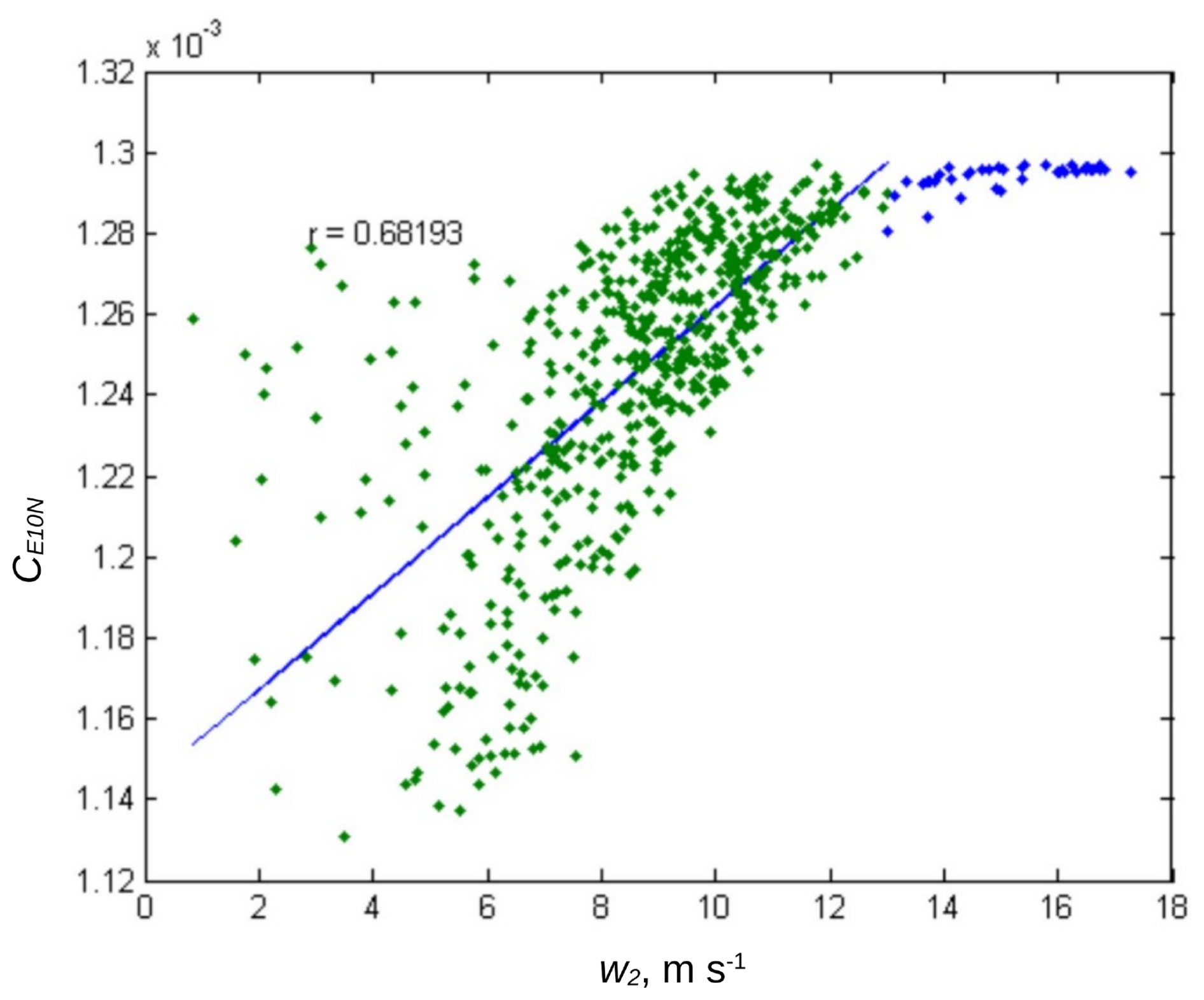
Figure 7 Dependence of the 10 m neutral transfer coefficient for moisture (C_E10N) on the 2 m wind speed (w₂) on the basis of 30 min mean values observed over Lake Zub/Priyadarshini (2017–2018).

Lake evaporation measured via the EC technique inherently includes contributions of both interfacial evaporation at the water surface and evaporation from spray air droplets. Although distinguishing between these two components is challenging, observations by Guest (2021) over the Southern Ocean suggest that under high-wind conditions, spray evaporation may account for approximately 18 % of interfacial evaporation. Consequently, if one wants to apply the wind dependent transfer coefficient (Eqs. 17 and 18) solely for the interfacial evaporation, the contribution of spray evaporation must be subtracted from the results. Furthermore, the stability dependence of the moisture transfer coefficient was found to be minor. This is primarily because the lakes consistently remained warmer than the ambient air during the period of the experiments (e.g., an average difference of 4.7 °C in January–February 2018). Consequently, under high-wind conditions, atmospheric stability remained near-neutral, rendering the transfer coefficient large and relatively insensitive to stability variations.

The actual values of the transfer coefficients (C_E and C_D) were estimated from EC measurements at Lake Glubokoe (2019–2020) using the methods described by Arya (1988) and Andreas (1986). In the first method (Eqs. 3–12), coefficients were estimated using roughness lengths derived from literature-based friction velocities (shown as black dots in Fig. 8). In the second method (Eqs. 13–14), transfer coefficients were calculated independently of atmospheric stability and friction velocity (shown as red dots in Fig. 8).

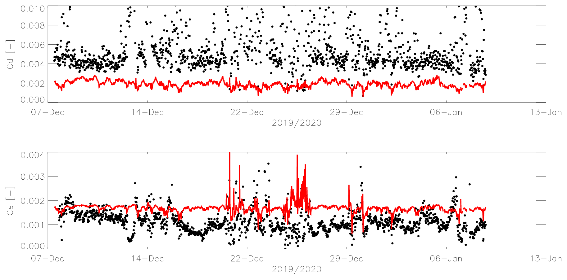
Figure 8 The actual values of the bulk transfer coefficients calculated following Arya (1988) (black dots) and Andreas (1986) (black dots) estimated from the EC measurement on Lake Glubokoe (2019–2020).

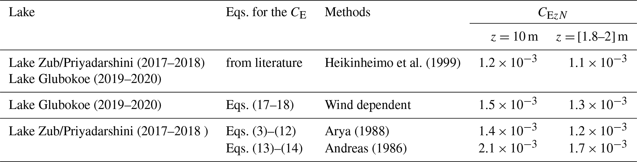
The actual values for C_E10 (normalized to a standard height of 10 m) varied between $\mathrm{1.2}\times {\mathrm{10}}^{-\mathrm{3}}$ and $\mathrm{2.1}\times {\mathrm{10}}^{-\mathrm{3}}$. Table 4 presents these values adjusted to our specific instrumentation heights: 2 m for Lake Zub/Priyadarshini and 1.8 m for Lake Glubokoe. These C_Ez values were subsequently used to calculate lake evaporation via Eq. (1). We evaluated the performance of the bulk-aerodynamic method with simulating hourly, daily, and seasonal cumulative evaporation totals based on the 30 min EC data.

Table 4 The equations applied in estimations the transfer coefficient (C_E) in the bulk-aerodynamic method. Notations: N refers to the neutral stratification, and z refers to the height of the instrument.

The hourly lake evaporation rate was simulated using the bulk-aerodynamic method, applying the transfer coefficients C_Ez  determined in Table 4. Figure 9 demonstrates strong agreement between the bulk-aerodynamic simulations and the independent eddy covariance (EC) measurements: the Pearson correlation coefficient is 0.92 for the data collected at Lake Zub/Priyadarshini during the 2017–2018 experiment (Fig. 9a) and 0.89 for Lake Glubokoe during the 2019–2020 experiment (Fig. 9b).

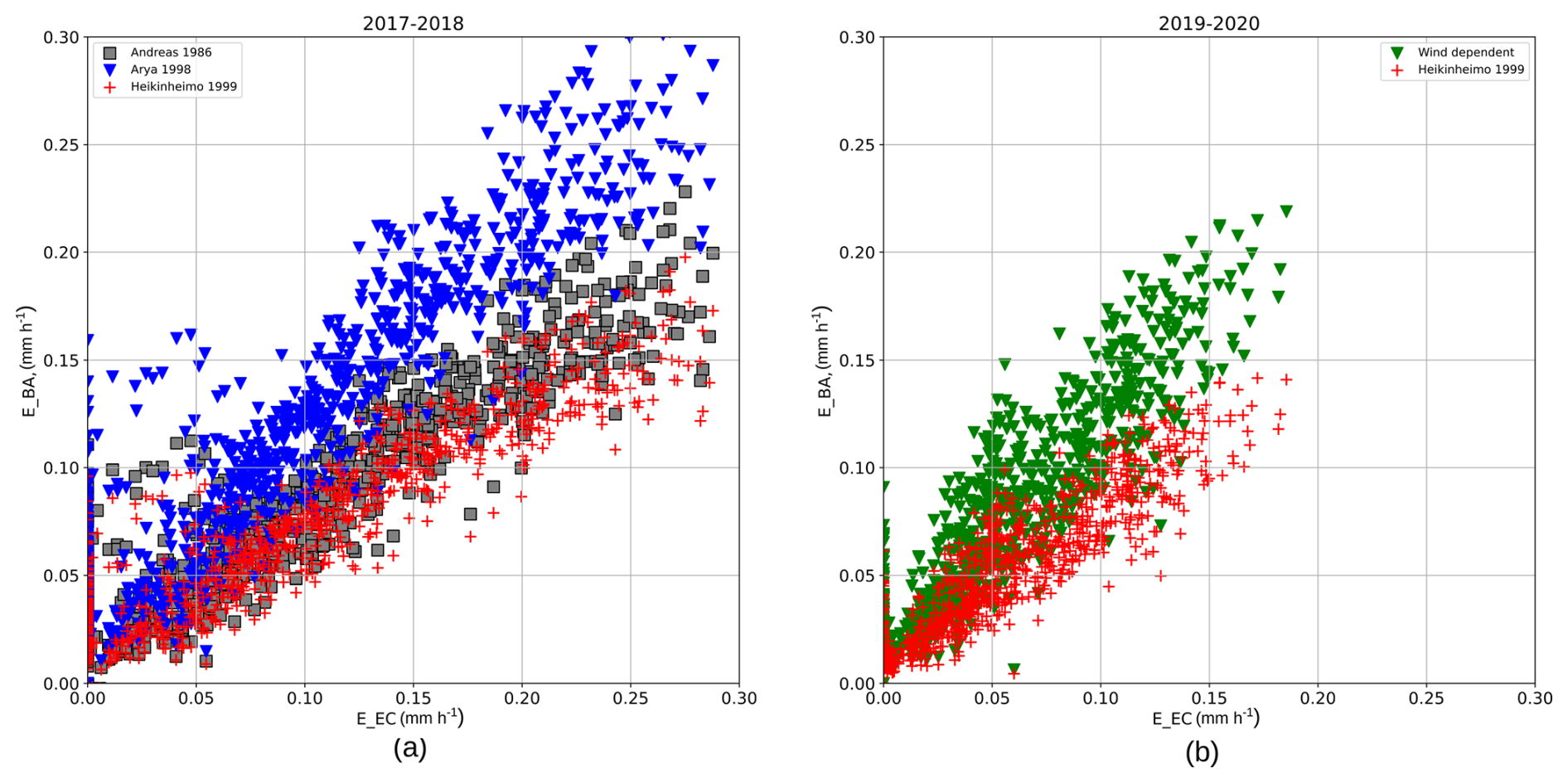
Figure 9 The measured (x axis) evaporation and simulated (y axis) with the bulk-aerodynamic method applying different actual values for the C_E: (a) Lake Zub/Priyadarshini and (b) Lake Glubokoe. The red dots cross to Heikinheimo et al. (1999), grey box to Andreas (1986), blue triangle to Arya (1988), and green triangle to the wind-dependent coefficient.

Lake evaporation is primarily driven by two factors: the vapour pressure deficit (which depends on the surface-air temperature gradient) and wind speed. Results from the two studied lakes indicate no significant dependency between lake evaporation and the vapour pressure deficit (Fig. 10a), with Pearson correlation coefficients near zero for both experimental periods (2017–2018 and 2019–2020). Conversely, a strong dependence was observed between lake evaporation and wind speed (Fig. 10b), with Pearson correlation coefficients of 0.58 for the ice-free Lake Zub/Priyadarshini (2017–2018) and 0.75 for the ice-covered Lake Glubokoe (2019–2020). These results imply that wind speed is the primary driver of evaporation for these lakes.

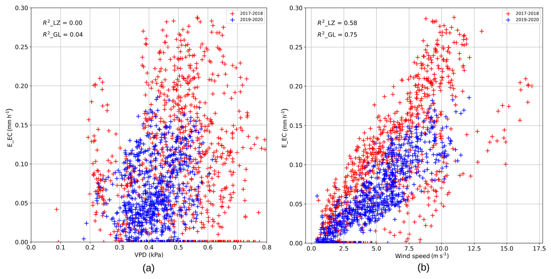
Figure 10 The scatter plots of the vapour pressure gradient, (x axis in a: VPD, kPa) and wind speed (x axis in b: m s⁻¹) against the hourly rate of lake evaporation (y axis in a and b) for Lake Zub/Priyadarshini (red) and Lake Glubokoe (blue).

The daily and seasonal rate of lake evaporation were calculated as the cumulative sum of hourly rate after the bulk-aerodynamic method using various C_E2 values. For the ice free Lake Zub/Priyadarshini (2017–2018), the mean daily evaporation rate varied between 2.0±0.1 and 3.0±0.2 mm d⁻¹ (Table 5). The best agreement with the EC technique (3.0±0.2 mm d⁻¹) was achieved using $C_{\mathrm{E}\mathrm{2}}=\mathrm{1.7}\times {\mathrm{10}}^{-\mathrm{3}}$. For Lake Glubokoe (2019–2020), the optimal estimate for the mean daily evaporation rate of 1.5±0.1 mm d⁻¹ is obtained using a transfer coefficient of $C_{\mathrm{E}\mathrm{2}}=\mathrm{1.2}\times {\mathrm{10}}^{-\mathrm{3}}$. This yields a daily lake evaporation rate of 1.6±0.1 mm d⁻¹, which is approximately 8 % lower than the reference (EC) method. Depending on the chosen value of C_E, the bulk-aerodynamic method either underestimated evaporation by up to 20 % (at $C_{\mathrm{E}\mathrm{2}}=\mathrm{1.1}\times {\mathrm{10}}^{-\mathrm{3}}$) or overestimated it by up to 38 % (using Eq. 17). The root-mean-square error varied between 0.4 and 0.8 mm d⁻¹, and the $s/\mathit{\sigma }$ ratio was 0.7 for C_E2 values of $\mathrm{1.2}\times {\mathrm{10}}^{-\mathrm{3}}$ and $\mathrm{1.7}\times {\mathrm{10}}^{-\mathrm{3}}$. These scores are considered acceptable for an indirect method, satisfying the criterion of $s/\mathit{\sigma }<\mathrm{0.8}$.

Table 5 The lake evaporation estimated using the bulk-aerodynamic method used different values of the transfer coefficient (C_E2). The bold numbers indicate the indirect method that yielded the estimates closest to the reference, and the parentheses show the verification with the independent data.

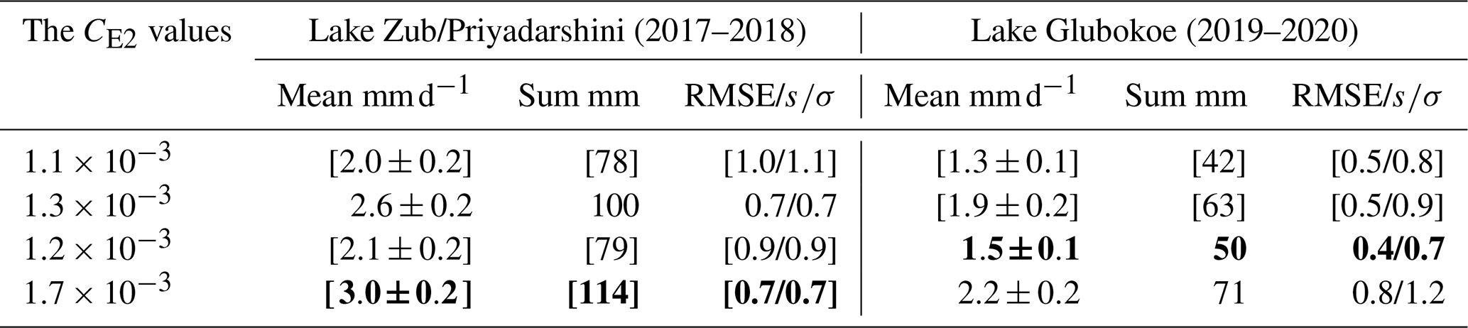
It is indeed interesting that the new wind-dependent transfer coefficient, derived on the basis of Lake Zub/Priyadarshini data, has a smaller RMSE for Lake Glubokoe than for Lake Zub/Priyadarshini. This is, however, understandable because the transfer coefficient is only one of the factors that controls the evaporation calculated using the bulk-aerodynamic formula. In addition to the transfer coefficient, at least the following factors may generate inaccuracy in the estimated evaporation: (1) errors in the measurements of lake surface temperature (controlling the saturation specific humidity), air specific humidity, and wind speed, (2) contribution of spray droplets to evaporation, (3) role of waves in the lake surface, and (4) validity of the Monin-Obukhov similarity theory, which requires quasi-stationary, horizontally homogeneous conditions. Errors and uncertainties associated with (1)–(4) above may either increase the overall error or partially offset one another. Hence, it is reasonable that the actual value of the transfer coefficient varies among lakes, as factors (1)–(4) may be site-specific, and also depends on the metrics used to evaluate performance (e.g., RMSE or $s/\mathit{\sigma })$.

5 Discussion

The eddy covariance technique is widely recognized as the most precise method for directly measuring evaporation over inland waters (Eugster et al., 1997; Rodrigues et al., 2020) and is commonly used as a reference to validate indirect methods (Tanny et al., 2008; Wang et al., 2019). However, its accuracy is sensitive to how the measurement system is deployed and post-processed (Burba, 2013; Spank et al., 2025). In our experiments, the EC system was deployed at low heights (1.8–2 m) to measure fluxes over the lake surface. The system was positioned to account for prevailing winds, and throughout the experiments, more than 80 % of the measured fluxes originated from the lake surface footprint. The EC measurements were processed using standard routines for open-path systems (filtering, gap filling, and footprint analysis). Therefore, we considered the EC measurements as the reference against which we compared the lake evaporation calculated via the indirect methods.

We estimated lake evaporation using eddy covariance measurements collected at two field experiments which spanned the ice break-up and ice-free periods for two glacial lakes differing in depths, volumes, and thermal regimes. For Lake Zub/Priyadarshini, direct estimates yielded a mean daily evaporation rate of 3.0±0.2 mm d⁻¹ during the ice-free period (January–February 2018). Daily evaporation rates ranged from 1.5 to 5.0 mm d⁻¹, with a cumulative total of 114 mm over the 38 d study period (1 January to 7 February 2018). Evaporation rates showed a strong positive correlation with wind speed, peaking at 5.0 mm d⁻¹ during storm events, with the highest values recorded on 2–3 January 2018. For Lake Glubokoe, daily evaporation rates varied between 0.3 and 3.2 mm d⁻¹, averaging 1.6±0.1 mm d⁻¹ during the ice break-up period. The cumulative evaporation for this 33 d period (December 2019–January 2020) was 54 mm, with the largest rates (up to 3.0 mm d⁻¹) observed during a storm on 13–15 December 2019. The EC measurements suggest that lakes begin significant evaporation immediately following break-up. The evaporation process is likely driven by strong and cold winds that maintain high evaporation rates even when the vapour pressure gradient is low.

To the best of our knowledge, measurements of lake evaporation in Antarctica using the EC technique have been conducted only at two lakes in the Schirmacher Oasis. However, such measurements are available for natural and artificial lakes globally (Guseva et al., 2023; Liu, 2023). While many studies analyse the surface energy budget of lakes, they typically report evaporation as a latent heat flux expressed in W m⁻² or J cm⁻² d⁻¹ (Stewart and Rouse, 1976; Stannard and Rosenberry, 1991; Blanken et al., 2000; Oswald and Rouse, 2004; Blanken et al., 2011). These energy-based units are impractical for hydrological (water balance) applications and are difficult to compare directly with evaporation depths measured by other techniques (e.g., evaporation pans). To ensure the comparability of our results, we converted the reported latent heat fluxes (W m⁻²) into equivalent depths of evaporated water.

Eddy covariance measurements remain rare for lakes located north of 60° latitude. Ala-Könni et al. (2022) measured evaporation over Lake Kuivajärvi (61° N, Finland) during the ice-free period, reporting a mean evaporation rate of 1.5–2.5 mm d⁻¹ during July–August; peak values of up to 5.0 mm d⁻¹ were observed during days with strong winds or when dry, cold synoptic fronts passed over the site. Blanken et al. (2000, 2003) measured evaporation over Great Slave Lake (62° N, Canada) during the ice-free periods from June to September (1997–1999), where evaporation rates reached 2.8 mm d⁻¹. Granger and Hedstrom (2011) estimated that the 4–9 d averaged evaporation rate reached 3.2–3.9 mm d⁻¹ during the ice-free period for small lakes situated next to Great Slave Lake. The northernmost EC measurements were collected from a small Arctic thermokarst lake (72° N, Russia) during an experiment spanning from April to August 2014 (Franz et al., 2018). In that study, the evaporation rate was near zero from April through mid-June (covering the ice-covered and break-up periods), subsequently averaging 2.5 mm d⁻¹ and peaking at 6.0 mm d⁻¹ during the ice-free period (July–September). These values are comparable to the evaporation rates observed over the ice-free Lake Zub/Priyadarshini in 2017–2018.

Evaporation from high-altitude lakes on the Qinghai-Tibetan Plateau (36° N, 3200–4700 m a.s.l., China) has been extensively studied over the last few decades, with EC measurements spanning more than five years (Wang et al., 2019; Gan and Liu, 2020; Meng et al., 2020; Shi et al., 2024). Li et al. (2016) found that evaporation over the ice-free Lake Qinghai reaches up to 12 mm d⁻¹ during storms, windy days (wind speed >4 m s⁻¹) contribute up to 22 % of the annual lake evaporation, and a contribution is controlled more by wind speed than by the vapour pressure gradient or solar radiation. This aligns with our results, which indicate that wind is the primary driver of evaporation over the two glacial lakes. Although we did not measure radiation during our experiments, such data are routinely collected by instrumentation installed at the Maitri and Novo observatories, offering opportunities for future research into the lake surface energy balance.

Faucher et al. (2019) measure ice sublimation over the surface of the perennially frozen Lake Untersee (71° S, Antarctica) using ablation stakes over a two-year period, estimating total sublimation (evaporation) between 400 to 750 mm yr⁻¹, which corresponds to a mean daily rate of 1.1–2.1 mm d⁻¹. These values are very close to the estimates obtained for the ice-covered Lake Glubokoe (2019–2020). Dugan et al. (2013) estimated lake ice ablation (sublimation) of 5–31 mm d⁻¹ for lakes in Tailor Valley (77° S, Antarctica); however, the authors were unable to distinguish between between the contributions of surface melt and sublimation to total ablation during the summer. For winter, Dugan et al. (2013) reported sublimation values ranging from 0.2 to 0.7 mm d⁻¹, which are naturally much smaller than we observed for fully or partially ice-free lakes. Leppäranta et al. (2016) reported summertime ice sublimation of 0.7 mm d⁻¹ for the lakes in the Vestfjella Mountains, Droning Maud Land (73° S, Antarctica), and ice thinning of 10–15 mm d⁻¹ on a small pond on a nunatak during days when winds speeds exceeded 30 m s⁻¹. As no surface melt occurred during these high-wind events, the observed ice thinning was attributed to sublimation (Leppäranta et al., 2016). Although no EC observations were available for that site, our calculations using the bulk-aerodynamic method confirm that these thinning rates are physically plausible under such extreme wind speeds, provided the ice surface temperature is near 0 °C and the air is very dry.

The bulk-aerodynamic method is highly sensitive to the moisture transfer coefficient (C_E) which is typically considered nearly constant at approximately $\mathrm{1.1}\times {\mathrm{10}}^{-\mathrm{3}}$ over the ocean (Kantha and Clayson, 2000) and varies between $\mathrm{1.1}\times {\mathrm{10}}^{-\mathrm{3}}$ and $\mathrm{2.4}\times {\mathrm{10}}^{-\mathrm{3}}$ over natural and artificial lakes (Hicks, 1972; Guseva et al., 2023). Our results indicate that the moisture transfer coefficient (C_E10N) varying between $\mathrm{1.4}\times {\mathrm{10}}^{-\mathrm{3}}$ for Lake Zub/Priyadarshini and $\mathrm{2.1}\times {\mathrm{10}}^{-\mathrm{3}}$ for Lake Glubokoe. Using these site-specific values, the bulk-aerodynamic method underestimated lake evaporation by 6 %–8 % with $s/\mathit{\sigma }<\mathrm{0.80}$ and RMSE of 0.6 mm d⁻¹. These metrics are within acceptable limits, supporting the use of this mass-transfer method to simulate hourly and daily lake evaporation rates in the Schirmacher Oasis. This aligns with conclusions from studies focusing on lake evaporation across the Qinghai-Tibetan Plateau (Wang et al., 2019).

The method used to calculate evaporation is particularly important for shallow Antarctic lakes, where water volume fluctuations are small throughout the summer season (Shevnina et al., 2021). Gopinath et al. (2020) demonstrated that summertime evaporation is a significant component of the water budget for shallow lakes in the Schirmacher Oasis, particularly Lake Zub/Priyadarshini. This lake serves as the freshwater supply for the Maitri research station, which hosts up to 25 people during the summer (COMNAP, 2017). The planned opening of the new Maitri-II research station in 2032 – designed to accommodate up to 140 people, and it needs additional freshwater. Dhote et al. (2021) evaluated the components of water balance equation for Lake Zub/Priyadarshini, identifying precipitation, inlet river runoff, and wastewater return as positive contributors, while outlet river runoff, evaporation, and freshwater withdrawal act as negative components. The volume of Lake Zub/Priyadarshini decreased by 40.3 m³ between January and February 2018, with a water balance equation residuals of 670.6 m³ (Dhote et al., 2021). The lake evaporation estimate of 58.5 m³ used by Dhote et al. (2021) was calculated following Odrova (1979), and this method underestimated the lake evaporation by 72 %. This corresponds to an absolute difference of approximately 42.1 m³, which accounts for roughly 6 % of the water balance residuals. This discrepancy could be mitigated by employing the bulk-aerodynamic method with a neutral 10 m moisture transfer coefficient (C_E10N) equalling $\mathrm{2.1}\times {\mathrm{10}}^{-\mathrm{3}}$. Meanwhile, the precipitation volume over Lake Zub/Priyadarshini during the same period was 5.3 m³, representing 0.05 % of the total lake volume. The remaining residual in the water balance is likely attributable to uncertainties in the methods used to evaluate inlet and outlet river runoff; our future research will specifically address these uncertainties.

6 Conclusions

We measured lake evaporation using the eddy covariance (EC) technique at two lakes in the Schirmacher Oasis (70° S), finding that summertime evaporation rates ranged from 0.3 to 5.0 mm d⁻¹. Depending on the presence of lake ice, mean evaporation varied from 1.6±0.1 mm d⁻¹ in the early stage of lake ice break-up (December) to 3.0±0.2 mm d⁻¹ during the ice-free period (January–February). Throughout the austral summer, the lakes remain warmer than the ambient air on most days. Variations in evaporation were primarily associated with changes in wind speed rather than fluctuations in the temperature gradient between the near-surface air and the lake surface water.

We further quantified the uncertainties of the bulk-aerodynamic method and five empirical formulas applied to estimate summertime evaporation over two lakes in coastal Antarctica. The bulk-aerodynamic method yielded the most accurate evaporation estimates (biases of 6 %–8 % for mean values) when the moisture transfer coefficient (C_E10N) was set to $\mathrm{1.4}\times {\mathrm{10}}^{-\mathrm{3}}$ for Lake Zub/Priyadarshini and $\mathrm{2.1}\times {\mathrm{10}}^{-\mathrm{3}}$ for Lake Glubokoe. This method demonstrated acceptable skill in estimating daily evaporation over both lakes during the ice break-up and open-water periods; consequently, it is recommended for hydrological (water balance) applications required for short-term operational decision-making. The selected empirical formulas underestimated daily evaporation over the lakes by 27 %–73 %. However, with appropriate corrections, they can be used to estimate cumulative summertime evaporation for hydrological applications. These indirect methods require measurements of lake surface water temperature that can be estimated, for example, from satellites equipped with thermal sensors.

The application of traditional approaches for measuring water balance components, including lake evaporation, is limited by the logistical challenges of maintaining and operating equipment in Antarctica. Determining accurate values for mass-transfer and empirical coefficients requires detailed hydrological and micrometeorological measurements, which are currently conducted only occasionally in this region. While isotope tracer-based approach can provide an accurate estimate of lake evaporation, it also requires regular water sampling as part of a unified monitoring program. Nevertheless, this method is relatively easier to implement on lakes located in the vicinity of settlements visiting by tourists.