Probabilistic hierarchical interpolation and interpretable neural network configurations for flood prediction

The past few years have witnessed the rise of neural networks (NNs) applications for hydrological time series modeling. By virtue of their capabilities, NN models can achieve unprecedented levels of performance when learning how to solve increasingly complex rainfall-runoff processes via data, making them pivotal for the development of computational hydrologic tasks such as flood predictions. The NN models should, to be considered practical, provide a probabilistic understanding of the model mechanisms and predictions and hints on what could perturb the model. In this paper, we developed two NN models, i.e., Neural Hierarchical Interpolation for Time Series Forecasting (N-HiTS) and Network-Based Expansion Analysis for Interpretable Time Series Forecasting (N-BEATS) with a probabilistic multi-quantile objective and benchmarked them with long short-term memory (LSTM) for flood prediction across two headwater streams in Georgia and North Carolina, USA. To generate a probabilistic prediction, a Multi-Quantile Loss was used to assess the 95th percentile prediction uncertainty (95 PPU) of multiple flooding events. Extensive experiments demonstrated the advantages of hierarchical interpolation and interpretable architecture, where both N-HiTS and N-BEATS provided an average accuracy improvement of ∼ 5 % over the LSTM benchmarking model. On a variety of flooding events, both N-HiTS and N-BEATS demonstrated significant performance improvements over the LSTM benchmark and showcased their probabilistic predictions by specifying a likelihood objective.

1 Introduction

The past few years have witnessed a rapid surge in the neural networks (NN) applications in hydrology. As these opaque, data-driven models are increasingly employed for critical hydrological predictions, the hydrology community has placed growing emphasis on developing trustworthy and interpretable NN models. However, maintaining coherence while producing accurate predictions can be a challenging problem (Olivares et al., 2024). There is a general agreement on the importance of providing probabilistic NN prediction (Sadeghi Tabas and Samadi, 2022), especially in the case of flood prediction (Martinaitis et al., 2023).

Flood occurrences have witnessed an alarming surge in frequency and severity globally. Jonkman (2005) studied a natural disaster database (Guha-Sapir and Below, 2002) and reported that over 27 years, more than 175 000 people died, and close to 2.2 billion were affected directly by floods worldwide. These numbers are likely an underestimation due to unreported events (Nevo et al., 2022). In addition, the United Nations Office for Disaster Risk Reduction reported that flooding has been the most frequent, widespread weather-related natural disaster since 1995, claiming over 600 000 lives, affecting around 4 billion people globally, and causing annual economic damage of more than 100 billion USD (UNISDR, 2015). This escalating trend has necessitated the need for better flood prediction and management strategies. Scholars have successfully implemented different flood models such as deterministic (e.g., Roelvink et al., 2009, Thompson and Frazier, 2014; Barnard et al., 2014; Erikson et al., 2018) and physically based flood models (e.g., Basso et al., 2016; Chen et al., 2016; Pourreza-Bilondi et al., 2017; Saksena et al., 2020; Refsgaard et al., 2022) in various environmental systems over the past several decades. These studies have heightened the need for precise flood prediction (Samadi et al., 2025), they have also unveiled limitations inherent in existing deterministic and physics-based models.

While evidence suggests that both deterministic and physics-based approaches are meaningful and useful (Sukovich et al., 2014; Zafarmomen et al., 2024), their forecasts rest heavily on imprecise and subjective expert opinion; there is a challenge for setting robust evidence-based thresholds to issue flood warnings and alerts (Palmer, 2012). Moreover, many of these traditional flood models, particularly physically explicit models, rely too strongly on a particular choice of numerical approximation and describe multiple process parameterizations only within a fixed spatial architecture (e.g., Clark et al., 2015). Recent NN models have shown promising results across a large variety of flood modeling applications (e.g., Nevo et al., 2022; Pally and Samadi, 2022; Dasgupta et al., 2023; Zhang et al., 2023b; Zafarmomen and Samadi, 2025; Saberian et al., 2026) and encourage the use of such methodologies as core drivers for neural flood prediction (Windheuser et al., 2023).

Earlier adaptations of these intelligent techniques showed promising for flood prediction (e.g., Hsu et al., 1995; Tiwari and Chatterjee, 2010). However, recent efforts have taken NN application to the next level, providing uncertainty assessment (Sadeghi Tabas and Samadi, 2022) and improvements over various spatio-temporal scales, regions, and processes (e.g., Kratzert et al., 2018; Park and Lee, 2024; Zhang et al., 2023a). Nevo et al. (2022) were the first scholars who employed long short-term memory (LSTM) for flood stage prediction and inundation mapping, achieving notable success during the 2021 monsoon season. Soon after, Russo et al. (2023) evaluated various NN models for predicting depth flood in urban systems, highlighting the potential of data-driven models for urban flood prediction. Similarly, Defontaine et al. (2023) emphasized the role of NN algorithms in enhancing the reliability of flood predictions, particularly in the context of limited data availability. Windheuser et al. (2023) studied flood gauge height forecasting using images and time series data for two gauging stations in Georgia, USA. They used multiple NN models such as Convolutional Neural Network (ConvNet/CNN) and LSTM to forecast floods in near real-time (up to 72 h).

In a sequence, Wee et al. (2023) used Impact-Based Forecasting (IBF) to propose a Flood Impact-Based Forecasting system (FIBF) using flexible fuzzy inference techniques, aiding decision-makers in a timely response. Zou et al. (2023) proposed a Residual LSTM (ResLSTM) model to enhance and address flood prediction gradient issues. They integrated Deep Autoregressive Recurrent (DeepAR) with four recurrent neural networks (RNNs), including ResLSTM, LSTM, Gated Recurrent Unit (GRU), and Time Feedforward Connections Single Gate Recurrent Unit (TFC-SGRU). They showed that ResLSTM achieved superior accuracy. While these studies reported the superiority of NN models for flood modeling, they highlighted a number of challenges, notably (i) the limited capability of proposed NN models to capture the spatial variability and magnitudes of extreme data over time, (ii) the lack of a sophisticated mechanism to capture different flood magnitudes and synthesize the prediction, and (iii) inability of the NN models to process data in parallel and capture the relationships between all elements in a sequential manner.

Recent advances in neural time series forecasting showed promising results that can be used to address the above challenges for flood prediction. Recent techniques include the adoption of the attention mechanism and Transformer-inspired approaches (Fan et al., 2019; Alaa and van der Schaar, 2019; Lim et al., 2021) along with attention-free architectures composed of deep stacks of fully connected layers (Oreshkin et al., 2020).

All these approaches are relatively easy to scale up in terms of flood magnitudes (small to major flood predictions), compared to LSTM and have proven to be capable of capturing spatiotemporal dependencies (Challu et al., 2022). In addition, these architectures can capture input-output relationships implicitly while they tend to be more computationally efficient. Many state-of-the-art NN approaches for flood forecasting have been established based on LSTM. There are cell states in the LSTM networks that can be interpreted as storage capacity often used in flood generation schemes. In LSTM, the updating of internal cell states (or storages) is regulated through several gates: the first gate regulates the storage depletion, the second one regulates storage fluctuations, and the third gate regulates the storages outflow (Tabas and Samadi, 2022). The elaborate gated design of the LSTM partly solves the long-term dependency problem in flood time series prediction (Fang et al., 2020), although, the structure of LSTMs is designed in a sequential manner that cannot directly connect two nonadjacent portions (positions) of a time series.

In this paper, we developed attention-free architecture, i.e. Neural Hierarchical Interpolation for Time Series Forecasting (N-HiTS; Challu et al., 2022) and Network-Based Expansion Analysis for Interpretable Time Series Forecasting (N-BEATS; Oreshkin et al., 2020) and benchmarked these models with LSTM for flood prediction. We developed fully connected N-BEATS and N-HiTS architectures using multi-rate data sampling, synthesizing the flood prediction outputs via multi-scale interpolation.

We implemented all algorithms for flood prediction on two headwater streams i.e., the Lower Dog River, Georgia, and the Upper Dutchmans Creek, North Carolina, USA to ensure that the results are reliable and comparable. The results of N-BEATS and N-HiTS techniques were compared with the benchmarking LSTM to understand how these techniques can improve the representations of rainfall and runoff dispensing over a recurrence process. Notably, this study represents a pioneering effort, as to the best of our knowledge, this is the first instance in which the application of N-BEATS and N-HiTS algorithms in the field of flood prediction has been explored. The scope of this research will focus on:

• i.

  Flood prediction in a hierarchical fashion with interpretable outputs: We built N-BEATS and N-HiTS for flood prediction with a very deep stack of fully connected layers to implicitly capture input-output relationships with hierarchical interpolation capabilities. The predictions also involve programming the algorithms with decreasing complexity and aligning their time scale with the final output through multi-scale hierarchical interpolation and interpretable architecture. Predictions were aggregated in a hierarchical fashion that enabled the building of a very deep neural network with interpretable configurations.

• ii.

  Uncertainty quantification of the models by employing probabilistic approaches: a Multi-Quantile Loss (MQL) was used to assess the 95th percentile prediction uncertainty (95 PPU) of multiple flooding events. MQL was integrated as the loss function to account for probabilistic prediction. MQL trains the model to produce probabilistic forecasts by predicting multiple quantiles of the distribution of future values.

• iii.

  Exploring headwater stream response to flooding: Understanding the dynamic response of headwater streams to flooding is essential for managing downstream flood risks. Headwater streams constitute the uppermost sections of stream networks, usually comprising 60 % to 80 % of a catchment area. Given this substantial coverage and the tendency for precipitation to increase with elevation, headwater streams are responsible for generating and controlling the majority of runoff in downstream portions (MacDonald and Coe, 2007).

The remainder of this paper is structured as follows. Section 2 presents the case study and data, NN models, performance metrics, and sensitivity and uncertainty approaches. Section 3 focuses on the results of flood predictions including sensitivity and uncertainty assessment and computation efficiency. Finally, Sect. 4 concludes the paper.

2 Methodology

2.1 Case Study and Data

This research used two headwater gauging stations located at the Lower Dog River watershed, Georgia (GA; USGS02337410, Dog River gauging station), and the Upper Dutchmans Creek watershed, North Carolina (NC; USGS0214269560, Killian Creek gauging station). As depicted in Fig. 1, the Lower Dog River and the Upper Dutchmans Creek watersheds are in the west and north parts of two metropolitan cities, Atlanta and Charlotte. The Lower Dog River stream gauge is established southeast of Villa Rica in Carroll County, where the USGS has regularly monitored discharge data since 2007 in 15 min increments. The Lower Dog River is a stream with a length of 15.7 miles (25.3 km; obtained from the U.S. Geological Survey [USGS] National Hydrography Dataset high-resolution flowline data), an average elevation of 851.94 m, and the watershed area above this gauging station is 66.5 square miles (172 km²; obtained from the Georgia Department of Natural Resources). This watershed is covered by 15.2 % residential area, 14.6 % agricultural land, and ∼ 70 % forest (Munn et al., 2020).

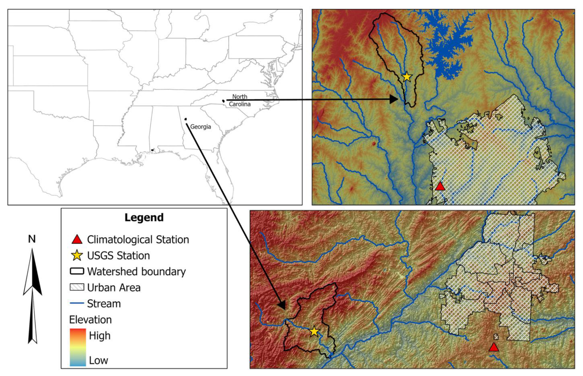
Figure 1 The Lower Dog River and The Upper Dutchmans Creek watersheds are in GA and NC. The proximity of the watersheds to Atlanta and Charlotte (urban area) are also displayed on the map.

Killian Creek gauging station at the Upper Dutchmans Creek watershed is established in Montgomery County, NC, where the USGS has regularly monitored discharge data since 1995 in 15 min increments. The Upper Dutchmans Creek is a stream with a length of 4.9 miles (7.9 km), an average elevation of 642.2 m (see Table 1), and the watershed area above this gauging station is 4 square miles (10.3 km²) with less than 3 % residential area and about 93 % forested land use (US EPA, 2024).

Table 1 The Lower Dog River and Upper Dutchmans Creek's physical characteristics.

The Lower Dog River has experienced significant flooding in the last decades. For example, in September 2009, the creek, along with most of northern GA, experienced heavy rainfall (5 inches, equal to 94 mm). The Lower Dog River, overwhelmed by large amounts of overland flow from saturated ground in the watershed, experienced massive flooding in September 2009 (Gotvald, 2010). The river crested at 33.8 feet (10.3 m) with a peak discharge of 59 900 cfs (1700 m³ s⁻¹), nearly six times the 100-year flood level (McCallum and Gotvald, 2010). In addition, Dutchmans Creek experienced significant flooding in February 2020. According to local news (WCCB Charlotte's CW, 2020), the flood in Gaston County caused significant infrastructure damage and community disruption. Key impacts included the threatened collapse of the Dutchman's Creek bridge in Mt. Holly and the closure of Highway 7 in McAdenville, GA.

To provide the meteorological forcing data, i.e., precipitation, temperature, and humidity, were extracted from the National Oceanic and Atmospheric Administration's (NOAA) Local Climatological Data (LCD). We used the NOAA precipitation, temperature, and humidity data of Atlanta Hartsfield Jackson International Airport and Charlotte Douglas Airport stations as an input for neural network algorithms. The data has been monitored since 1 January 1948, and 22 July 1941, with an hourly interval which was used as an input variable for constructing neural networks.

To fill in the missing values in the data, we used the spline interpolation method. We applied this method to fill the gaps in time series data, although the missing values were insignificant (less than 1 %). In addition, we employed the Minimum Inter-Event Time (MIT) approach to precisely identify and separate individual storm events. The MIT-based event delineation is pivotal for accurately defining storm events. This method allowed us to isolate discrete rainfall episodes, aiding a comprehensive analysis of storm events. Moreover, it provided a basis for event-specific examination of flood responses, such as initial condition and cessation (loss), runoff generation, and runoff dynamics.

The hourly rainfall dataset consists of distinct rainfall occurrences, some consecutive and others clustered with brief intervals of zero rainfall. As these zero intervals extend, we aim to categorize them into distinct events. It's worth noting that even within a single storm event, we often encounter short periods of no rainfall, known as intra-storm zero values. In the MIT method, we defined a storm event as a discrete rainfall episode surrounded by dry periods both preceding and following it, determined by an MIT (Asquith et al., 2005; Safaei-Moghadam et al., 2023).

There are many ways to determine MIT value. One practical approximation is using serial autocorrelation between rainfall occurrences. MIT approach uses autocorrelation that measures the statistical dependency of rainfall data at one point in time with data at earlier, or lagged times within the time series. The lag time represents the gap between data points being correlated. When the lag time is zero, the autocorrelation coefficient is unity, indicating a one-to-one correlation. As the lag time increases, the statistical correlation diminishes, converging to a minimum value. This signifies the fact that rainfall events become progressively less statistically dependent or, in other words, temporally unrelated. To pinpoint the optimal MIT, we analyzed the autocorrelation coefficients for various lag times, observing the point at which the coefficient approaches zero. This lag time signifies the minimum interval of no rainfall, effectively delineating distinct rainfall events.

2.2 NN Algorithms

In this study, three distinct neural network (NN) architectures were developed to perform multi-horizon flood forecasting. Each NN was coupled with a MQL objective to generate probabilistic predictions and quantify predictive uncertainty. Throughout the manuscript, the term parameters are used exclusively to refer to the network's weights and biases for clarity and consistency.

2.2.1 LSTM

LSTM is an RNN architecture widely used as a benchmark model for flood neural time series modeling. LSTM networks are capable of selectively learning order dependence in sequence prediction problems (Sadeghi Tabas and Samadi, 2022). These networks are powerful because they can capture the temporal features, especially the long-term dependencies (Hochreiter et al., 2001) and are independent of the length of the data sequences input, meaning that each sample is independent from another one.

The memory cell state within LSTM plays a crucial role in capturing extended patterns in data, making it well-suited for dynamic time series modeling such as flood prediction. An LSTM cell uses the following functions to compute flood prediction.

$$\begin{array}{}\text{(1)}& {\displaystyle }{i}_t=\mathit{\sigma }\left(A_i{x}_t+B_i{h}_{t-\mathrm{1}}+c_i\right)\text{(2)}& {\displaystyle }{f}_t=\mathit{\sigma }(A_f{x}_t+B_f{h}_{t-\mathrm{1}}+c_f)\text{(3)}& {\displaystyle }{o}_t=\mathit{\sigma }(A_{\mathrm{o}}{x}_t+B_{\mathrm{o}}{h}_{t-\mathrm{1}}+c_{\mathrm{o}})\text{(4)}& {\displaystyle }{m}_t=f_t\odot m_{t-\mathrm{1}}+i_t\odot \tanh (A_g{x}_t+B_g{h}_{t-\mathrm{1}}+c_g)\text{(5)}& {\displaystyle }{h}_t=o_t\odot \tanh \left(m_t\right)\end{array}$$

Where x_t and h_t represent the input and the hidden state at time step t, respectively. ⊙ denotes element-wise multiplication, tanh stands for the hyperbolic tangent activation function, and σ represents the sigmoid activation function. A, B, and c are trainable weights and biases that undergo optimization during the training process. m_t and h_t are cell states at time step t that are employed in the input processing for the next time step. m_t represents the memory state responsible for preserving long-term information, while h_t represents the memory state preserving short-term information. The LSTM cell consists of a forget gate f_t, an input gate i_t and an output gate o_t and has a cell state m_t. At every time step t, the cell gets the data point x_t with the output of the previous cell h_t−1 (Windheuser et al., 2023). The forget gate then defines if the information is removed from the cell state, while the input gate evaluates if the information should be added to the cell state and the output gate specifies which information from the cell state can be used for the next cells.

We used two LSTM layers with 128 cells in the first two hidden layers as encoder layers, which were then connected to two multilayer perceptron (MLP) layers with 128 neurons as decoder layers. The LSTM simulation was performed with these input layers along with the Adam optimizer (Kingma and Ba, 2017), tanh activation function, and a single lagged dependent-variable value to train with a learning rate of 0.001. The architecture of the proposed LSTM model is illustrated in Fig. 2.

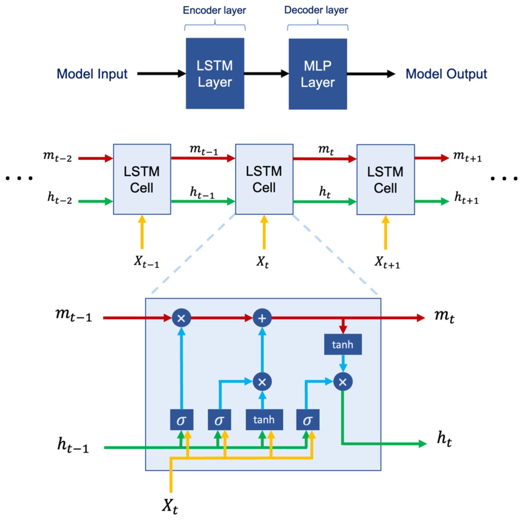
Figure 2 The structure of LSTM programmed in this research. We used tanh and sigmoid as activation functions along with 2 layers of LSTM, 2 layers of MLP, and 128 cells in each layer.

2.2.2 N-BEATS

N-BEATS is a deep learning architecture based on backward and forward residual links and the very deep stack of fully connected layers specifically designed for sequential data forecasting tasks (Oreshkin et al., 2020). This architecture has several desirable properties including interpretability. The N-BEATS architecture distinguishes itself from existing architecture in several ways. First, the algorithm approaches forecasting as a non-linear multivariate regression problem instead of a sequence-to-sequence challenge. Indeed, the core component of this architecture (as depicted in Fig. 3) is a fully connected non-linear regressor, which takes the historical data from a time series as input and generates multiple data points for the forecasting horizon. Second, most existing time series architectures are quite limited in depth, typically consisting of one to five LSTM layers. N-BEATS employs the residual principle to stack a substantial number of layers together, as illustrated in Fig. 3. In this configuration, the basic block not only predicts the next output but also assesses its contribution to decomposing the input, a concept that is referred to as “backcast” (see Oreshkin et al., 2020).

Figure 3 The N-BEATS modeling structure, used in this research.

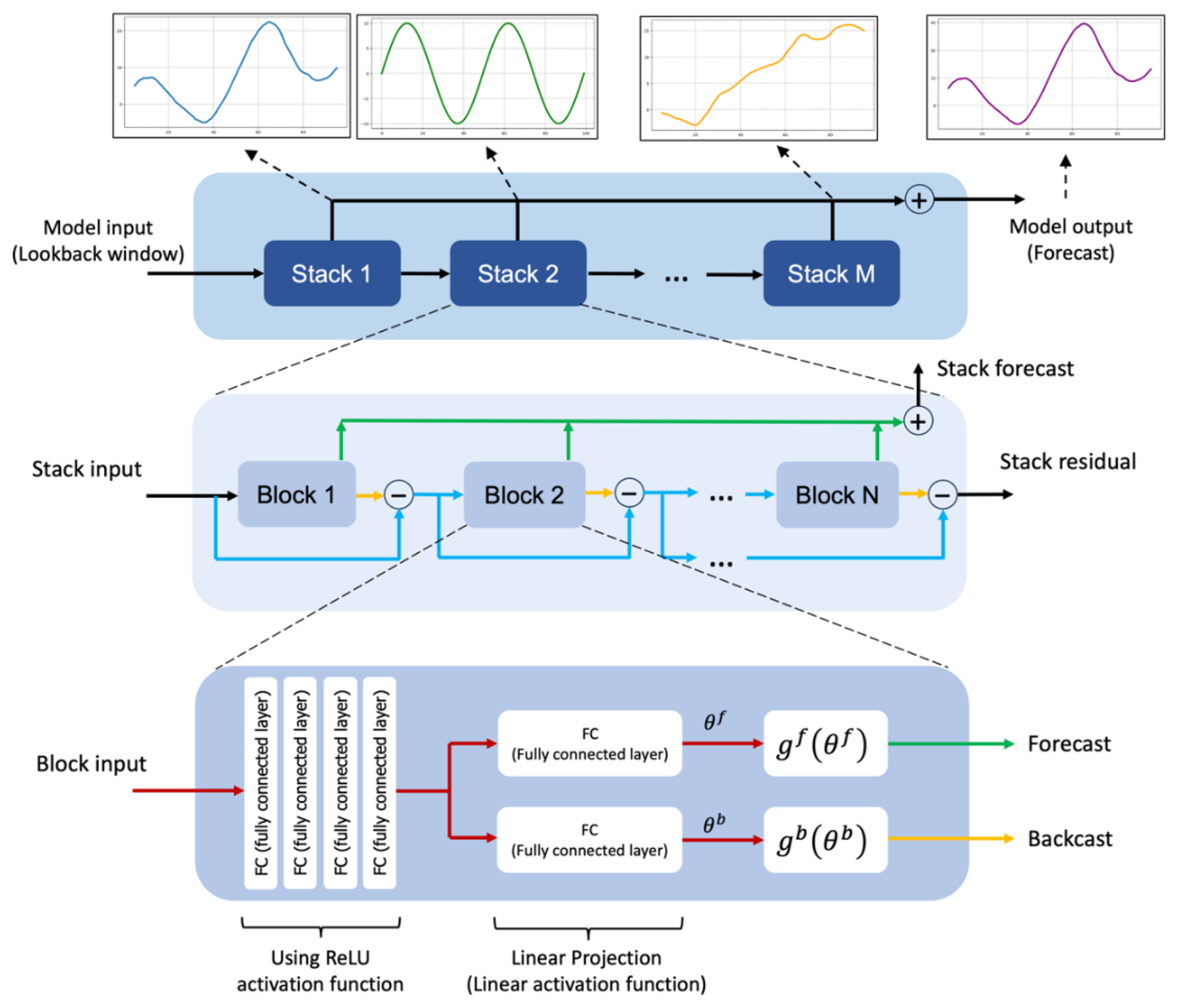
The basic building block in the architecture features a fork-like structure, as illustrated in Fig. 3 (bottom). The lth block (for the sake of brevity, the block index l is omitted from Fig. 3) takes its respective input, x_l, and produces two output vectors: ${\widehat{\mathit{x}}}_l$ and ${\widehat{\mathit{y}}}_l$. In the initial block of the model, x_l corresponds to the overall model input, which is a historical lookback window of a specific length, culminating with the most recent observed data point. For the subsequent blocks, x_l is derived from the residual outputs of the preceding blocks. Each block generates two distinct outputs: (1) ${\widehat{\mathit{y}}}_l$: This represents the forward forecast of the block, spanning a duration of H time units. (2) ${\widehat{\mathit{x}}}_l$: This signifies the block's optimal estimation of x_l, which is referred to “backcast.” This estimation is made within the constraints of the functional space available to the block for approximating signals (Oreshkin et al., 2020).

Internally, the fundamental building block is composed of two elements. The initial element involves a fully connected network, which generates forward expansion coefficient predictors, ${\mathit{\theta }}_l^{\mathrm{f}}$, and a backward expansion coefficient predictor, ${\mathit{\theta }}_l^{\mathrm{b}}$. The second element encompasses both backward basis layers, $g_l^{\mathrm{b}}$, and forward basis layers, $g_l^{\mathrm{f}}$. These layers take the corresponding forward ${\mathit{\theta }}_l^{\mathrm{f}}$and backward ${\mathit{\theta }}_l^{\mathrm{b}}$expansion coefficients as input, conduct internal transformations using a set of basis functions, and ultimately yield the backcast, ${\widehat{\mathit{x}}}_l$, and the forecast outputs, ${\widehat{\mathit{y}}}_l$, as previously described by Oreshkin et al. (2020). The following equations describe the first element:

$$\begin{array}{}\text{(6)}& {\displaystyle }\begin{array}{rl}{h}_{l,\mathrm{1}}& ={\mathrm{FC}}_{l,\mathrm{1}}\left(x_l\right),h_{l,\mathrm{2}}={\mathrm{FC}}_{l,\mathrm{2}}\left(h_{l,\mathrm{1}}\right),\\ & h_{l,\mathrm{3}}={\mathrm{FC}}_{l,\mathrm{3}}\left(h_{l,\mathrm{2}}\right),h_{l,\mathrm{4}}={\mathrm{FC}}_{l,\mathrm{4}}\left(h_{l,\mathrm{3}}\right)\end{array}\text{(7)}& {\displaystyle }{\mathit{\theta }}_l^{\mathrm{b}}={\mathrm{LINEAR}}_l^{\mathrm{b}}\left(h_{l,\mathrm{4}}\right),{\mathit{\theta }}_l^{\mathrm{b}}={\mathrm{LINEAR}}_l^{\mathrm{b}}\left(h_{l,\mathrm{4}}\right)\end{array}$$

The LINEAR layer, in essence, functions as a straightforward linear projection, meaning ${\mathit{\theta }}_l^{\mathrm{f}}=W_l^{\mathrm{f}}{h}_{l,\mathrm{4}}$. As for the fully connected (FC) layer, it takes on the role of a conventional FC layer, incorporating RELU non-linearity as an activation function.

The second element performs the mapping of expansion coefficients ${\mathit{\theta }}_l^{\mathrm{f}}$and ${\mathit{\theta }}_l^{\mathrm{b}}$ to produce outputs using basis layers, resulting in ${\widehat{\mathit{y}}}_l=g_l^{\mathrm{f}}\left({\mathit{\theta }}_l^{\mathrm{f}}\right)$ and ${\widehat{\mathit{x}}}_l=g_l^{\mathrm{b}}\left({\mathit{\theta }}_l^{\mathrm{b}}\right)$. This process is defined by the following equation:

$$\begin{array}{}\text{(8)}& {\widehat{\mathit{y}}}_l=\sum _{i=\mathrm{1}}^{\dim \left({\mathit{\theta }}_l^{\mathrm{f}}\right)}{\mathit{\theta }}_{l,i}^{\mathrm{f}}{\mathit{v}}_i^{\mathrm{f}},{\widehat{\mathit{x}}}_l=\sum _{i=\mathrm{1}}^{\dim \left({\mathit{\theta }}_l^{\mathrm{b}}\right)}{\mathit{\theta }}_{l,i}^{\mathrm{b}}{\mathit{v}}_i^{\mathrm{b}}\end{array}$$

Within this context, ${\mathit{v}}_i^{\mathrm{f}}$ and ${\mathit{v}}_i^{\mathrm{b}}$ represent the basis vectors for forecasting and backcasting, respectively, while ${\mathit{\theta }}_{l,i}^{\mathrm{f}}$ corresponds to the ith element of ${\mathit{\theta }}_l^{\mathrm{f}}$.

The N-BEATS uses a novel hierarchical doubly residual architecture which is illustrated in Fig. 3 (top and middle). This framework incorporates two residual branches, one traversing the backcast predictions of each layer, while the other traverses the forecast branch of each layer. The following equation describes this process:

$$\begin{array}{}\text{(9)}& x_l=x_{l-\mathrm{1}}-{\widehat{x}}_{l-\mathrm{1}}\widehat{y}=\sum _l{\widehat{\mathit{y}}}_l\end{array}$$

As mentioned earlier, in the specific scenario of the initial block, its input corresponds to the model-level input x. In contrast, for all subsequent blocks, the backcast residual branch x_l can be conceptualized as conducting a sequential analysis of the input signal. The preceding block eliminates the portion of the signal ${\widehat{x}}_{l-\mathrm{1}}$ that it can effectively approximate, thereby simplifying the prediction task for downstream blocks. Significantly, each block produces a partial forecast ${\widehat{\mathit{y}}}_l$ , which is initially aggregated at the stack level and subsequently at the overall network level, establishing a hierarchical decomposition. The ultimate forecast $\widehat{y}$ is the summation of all partial forecasts (Oreshkin et al., 2020).

The N-BEATS model has two primary configurations: generic and interpretable. These configurations determine how the model structures its blocks and how it processes time series data. In the generic configuration, the model uses a stack of generic blocks that are designed to be flexible and adaptable to various patterns in the time series data. Each generic block consists of fully connected layers with ReLU activation functions. The key characteristic of generic configuration is its flexibility. Since the blocks are not specialized for any specific pattern (like trend or seasonality), they can learn a wide range of patterns directly from the data (Oreshkin et al., 2020). In the interpretable configuration, the model architecture integrates distinct trend and seasonality components. This involves structuring the basis layers at the stack level specifically to model these elements, allowing the stack outputs to be more easily understood.

Trend Model: In this stack $g_{s,l}^{\mathrm{b}}$ and $g_{s,l}^{\mathrm{f}}$ are polynomials of a small degree p, functions that vary slowly across the forecast window, to replicate monotonic or slowly varying nature of trends:

$$\begin{array}{}\text{(10)}& {\widehat{y}}_{s,l}=\sum _{i=\mathrm{0}}^p{\mathit{\theta }}_{s,l,i}^{\mathrm{f}}{t}^i\end{array}$$

The time vector $\mathit{t}=[\mathrm{0},\mathrm{1},\mathrm{2},\mathrm{\dots },H-\mathrm{2},H-\mathrm{1}{]}^T/H$ is specified on a discrete grid ranging from 0 to $(H-\mathrm{1})/H$, projecting H steps into the future. Consequently, the trend forecast represented in matrix form is:

$$\begin{array}{}\text{(11)}& {\widehat{y}}_{s,l}^{\mathrm{tr}}=\mathbf{T}{\mathit{\theta }}_{s,l}^{\mathrm{f}}\end{array}$$

Where the polynomial coefficients, ${\mathit{\theta }}_{s,l}^{\mathrm{f}}$, predicted by an FC network at layer l of stack s, are described by Eqs. (6) and (7). The matrix T, consisting of powers of t, is represented as $[\mathrm{1},t,\mathrm{\dots },t^p]$. When p is small, such as 2 or 3, it compels ${\widehat{y}}_{s,l}^{\mathrm{tr}}$ to emulate a trend (Oreshkin et al., 2020).

Seasonality model: In this stack $g_{s,l}^{\mathrm{b}}$ and $g_{s,l}^{\mathrm{f}}$ are periodic functions, to capture the cyclical and recurring characteristics of seasonality, such that $y_t=y_{t-\mathrm{\Delta }}$, where Δ is the seasonality period. The Fourier series serves as a natural foundation for modeling periodic functions:

$$\begin{array}{}\text{(12)}& {\widehat{y}}_{s,l}=\sum _{i=\mathrm{0}}^{\frac{H}{\mathrm{2}}-\mathrm{1}}{\mathit{\theta }}_{s,l,i}^{\mathrm{f}}\cos \left(\mathrm{2}\mathit{\pi }it\right)+{\mathit{\theta }}_{s,l,i+[H/\mathrm{2}]}^{\mathrm{f}}\sin \left(\mathrm{2}\mathit{\pi }it\right)\end{array}$$

Consequently, the seasonality forecast is represented in the following matrix form:

$$\begin{array}{}\text{(13)}& {\displaystyle }{\widehat{y}}_{s,l}^{\mathrm{seas}}=S{\mathit{\theta }}_{s,l}^{\mathrm{f}}\text{(14)}& {\displaystyle }\begin{array}{rl}\mathbf{S}& =[\mathrm{1},\cos (\mathrm{2}\mathit{\pi }t),\mathrm{\dots },\cos \left(\mathrm{2}\mathit{\pi }\left[{\displaystyle \frac{H}{\mathrm{2}}}-\mathrm{1}\right]t\right),\\ & \sin \left(\mathrm{2}\mathit{\pi }t\right),\mathrm{\dots },\sin \left(\mathrm{2}\mathit{\pi }\left[{\displaystyle \frac{H}{\mathrm{2}}}-\mathrm{1}\right]t\right)\end{array}\end{array}$$

Where the Fourier coefficients ${\mathit{\theta }}_{s,l}^{\mathrm{f}}$, that predicted by an FC network at layer l of stack s, are described by Eqs. (6) and (7). The matrix S represents sinusoidal waveforms. As a result, the forecast ${\widehat{y}}_{s,l}^{\mathrm{seas}}$ becomes a periodic function that imitates typical seasonal patterns (Oreshkin et al., 2020).

2.2.3 N-HiTS

N-HiTS builds upon the N-BEATS architecture but with improved accuracy and computational efficiency for long-horizon forecasting. N-HiTS utilizes multi-rate sampling and multi-scale synthesis of forecasts, leading to a hierarchical forecast structure that lowers computational demands and improves prediction accuracy (Challu et al., 2022).

Like N-BEATS, N-HiTS employs local nonlinear mappings onto foundational functions within numerous blocks (illustrated in Fig. 4). Each block includes an MLP that generates backcast and forecast output coefficients. The backcast output refines the input data for the following blocks, and the forecast outputs are combined to generate the final prediction. Blocks are organized into stacks, with each stack dedicated to grasping specific data attributes using its own distinct set of functions. The network's input is a sequence of L lags (look-back period), with S stacks, each containing B blocks (Challu et al., 2022).

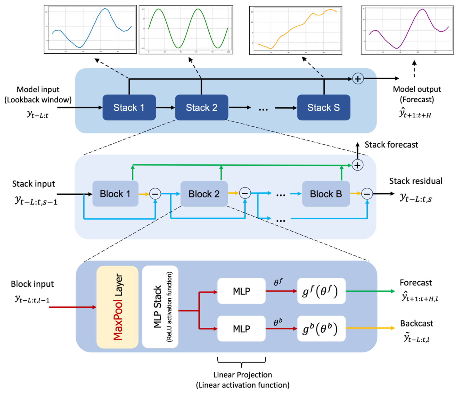
Figure 4 The structure of N-HiTS model programmed in this study. The architecture includes several Stacks, each Stack includes several Block, where each block consists of a MaxPool layer and a multi-layer which learns to produce coefficients for the backcast and forecast outputs of its basis.

In each block, a MaxPool layer with varying kernel sizes (k_l) is employed at the input, enabling the block to focus on specific input components of different scales. Larger kernel sizes emphasize the analysis of larger-scale, low-frequency data, aiding in improving long-term forecasting accuracy. This approach, known as multi-rate signal sampling, alters the effective input signal sampling rate for each block's MLP (Challu et al., 2022).

Additionally, multi-rate processing has several advantages. It reduces memory usage, computational demands, and the number of learnable parameters, and helps prevent overfitting, while preserving the original receptive field. The following operation is applicable to the input $y_{t-L:t,l}$ of each block, with the first block (l=1) using the network-wide input, where $y_{t-L:t,\mathrm{1}}\equiv y_{t-L:t}$.

$$\begin{array}{}\text{(15)}& y_{t-L:t,l}=\mathrm{MaxPool}(y_{t-L:t,l},k_l)\end{array}$$

In many multi-horizon forecasting models, the number of neural network predictions matches the horizon's dimensionality, denoted as H. For instance, in N-BEATS, the number of predictions $\left|{\mathit{\theta }}_l^{\mathrm{f}}\right|=H$. This results in a significant increase in computational demands and an unnecessary surge in model complexity as the horizon H becomes larger (Challu et al., 2022).

To address these challenges, N-HiTS proposes the use of temporal interpolation. This model manages the parameter counts per unit of output time ($\left|{\mathit{\theta }}_l^{\mathrm{f}}\right|=⌈r_{l}H⌉$) by defining the dimensionality of the interpolation coefficients with respect to the expressiveness ratio r_l. To revert to the original sampling rate and predict all horizon points, this model employs temporal interpolation through the function g:

$$\begin{array}{}\text{(16)}& {\displaystyle }{\widehat{y}}_{\mathit{\tau },l}=g\left(\mathit{\tau },{\mathit{\theta }}_l^{\mathrm{f}}\right),\forall \mathit{\tau }\in \mathit{\{}t+\mathrm{1},\mathrm{\dots },t+H\mathit{\}},\text{(17)}& {\displaystyle }{\stackrel{\mathrm{̃}}{y}}_{\mathit{\tau },l}=g\left(\mathit{\tau },{\mathit{\theta }}_l^{\mathrm{b}}\right),\forall \mathit{\tau }\in \mathit{\{}t-L,\mathrm{\dots },t\mathit{\}},\text{(18)}& {\displaystyle }g\left(\mathit{\tau },\mathit{\theta }\right)=\mathit{\theta }\left[t_{\mathrm{1}}\right]+\left({\displaystyle \frac{\mathit{\theta }\left[t_{\mathrm{2}}\right]-\mathit{\theta }\left[t_{\mathrm{1}}\right]}{t_{\mathrm{2}}-t_{\mathrm{1}}}}\right)(\mathit{\tau }-t_{\mathrm{1}})\text{(19)}& {\displaystyle }{t}_{\mathrm{1}}=\arg \underset{t\in \mathit{\tau }:t\le \mathit{\tau }}{min}\mathit{\tau }-t,t_{\mathrm{2}}=t_{\mathrm{1}}+\mathrm{1}/r_l\end{array}$$

The hierarchical interpolation approach involves distributing expressiveness ratios over blocks, integrated with multi-rate sampling. Blocks closer to the input employ more aggressive interpolation, generating lower granularity signals. These blocks specialize in analyzing more aggressively subsampled signals. The final hierarchical prediction, ${\widehat{y}}_{t+\mathrm{1}:t+H}$, is constructed by combining outputs from all blocks, creating interpolations at various time-scale hierarchy levels. This approach maintains a structured hierarchy of interpolation granularity, with each block focusing on its own input and output scales (Challu et al., 2022).

To manage a diverse set of frequency bands while maintaining control over the number of parameters, exponentially increasing expressiveness ratios are recommended. As an alternative, each stack can be dedicated to modeling various recognizable cycles within the time series (e.g., weekly, or daily) employing matching r_l. Ultimately, the residual obtained from backcasting in the preceding hierarchy level is subtracted from the input of the subsequent level, intensifying the next-level block's attention on signals outside the previously addressed band (Challu et al., 2022).

$$\begin{array}{}\text{(20)}& {\displaystyle }{\widehat{y}}_{t+\mathrm{1}:t+H}=\sum _{l=\mathrm{1}}^L{\widehat{y}}_{t+\mathrm{1}:t+H,l}\text{(21)}& {\displaystyle }{y}_{t-L:t,l+\mathrm{1}}=y_{t-L:t,l}-{\stackrel{\mathrm{̃}}{y}}_{t-L:t,l}\end{array}$$

2.3 Performance Metrics

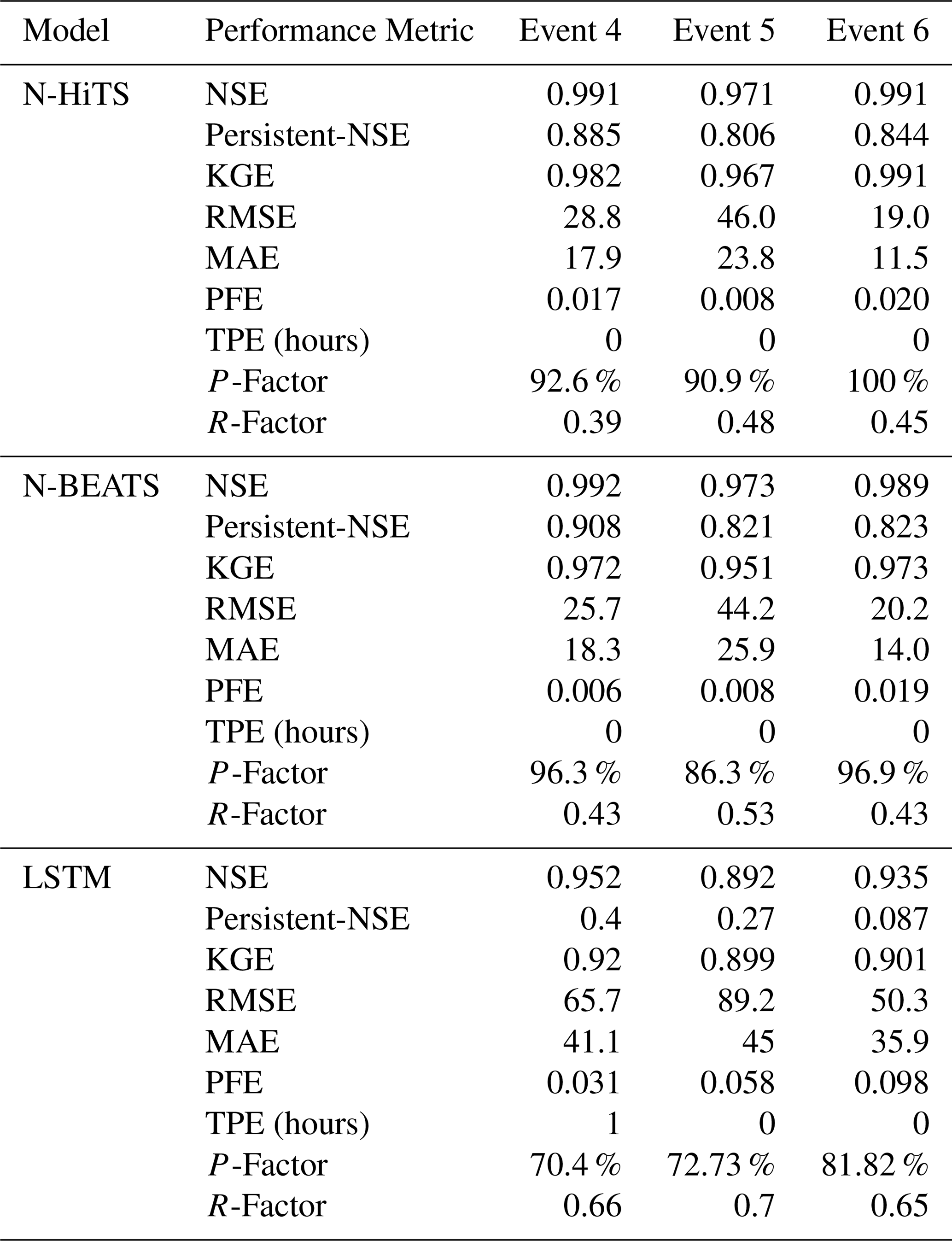
To comprehensively evaluate the accuracy of flood predictions, we utilized a suite of metrics, including Nash-Sutcliffe Efficiency (NSE; Nash and Sutcliffe, 1970), persistent Nash-Sutcliffe Efficiency (persistent-NSE), Kling–Gupta efficiency (KGE; Gupta et al., 2009), Root Mean Square Error (RMSE), Mean Absolute Error (MAE), Peak Flow Error (PFE), and Time to Peak Error (TPE; Evin et al., 2024; Lobligeois et al., 2014). These metrics collectively facilitate a rigorous assessment of the model's performance in reproducing the magnitude of observed peak flows and the shape of the hydrograph.

NSE measures the model's ability to explain the variance in observed data and assesses the goodness-of-fit by comparing the observed and simulated hydrographs. In hydrological studies, the NSE index is a widely accepted measure for evaluating the fitting quality of models (McCuen et al., 2006). It is calculated as:

$$\begin{array}{}\text{(22)}& \mathrm{NSE}=\mathrm{1}-{\displaystyle \frac{{\sum }_{i=\mathrm{1}}^n{\left(Q_{s_i}-Q_{o_i}\right)}^{\mathrm{2}}}{{\sum }_{i=\mathrm{1}}^n{\left(Q_{o_i}-\stackrel{\mathrm{‾}}{Q_{\mathrm{o}}}\right)}^{\mathrm{2}}}}\end{array}$$

Where $Q_{o_i}$ represents observed value at time i, $Q_{s_i}$ represents simulated value at time i, $\stackrel{\mathrm{‾}}{Q_{\mathrm{o}}}$ is the mean observed values and n is the number of data points. An NSE value of 1 indicates a perfect match between the observed and modeled data, while lower values represent the degree of departure from a perfect fit.

As the models are designed to predict one hour ahead in one of the prediction horizons, the persistent-NSE is essential for evaluating their performance. The standard NSE measures the model's sum of squared errors relative to the sum of squared errors when the mean observation is used as the forecast value. In contrast, persistent-NSE uses the most recent observed data as the forecast value for comparison (Nevo et al., 2022). The persistent-NSE is calculated as:

$$\begin{array}{}\text{(23)}& \text{persistent-NSE}=\mathrm{1}-{\displaystyle \frac{{\sum }_{i=\mathrm{1}}^n{\left(Q_{s_i}-Q_{o_i}\right)}^{\mathrm{2}}}{{\sum }_{i=\mathrm{1}}^n{\left(Q_{o_i}-Q_{o_{i-\mathrm{1}}}\right)}^{\mathrm{2}}}}\end{array}$$

Where $Q_{o_i}$ represents the observed value at time i, $Q_{s_i}$ represents the simulated value at time i, $Q_{o_{i-\mathrm{1}}}$is the observed value at the last time step (i−1) and n is the number of data points.

The KGE is a widely used performance metric in hydrological modeling and combines multiple aspects of model performance, including correlation, variability bias, and mean bias. The KGE metric is calculated using the following equation:

$$\begin{array}{}\text{(24)}& \mathrm{KGE}=\mathrm{1}-\sqrt{(r-\mathrm{1}{)}^{\mathrm{2}}+(\mathit{\alpha }-\mathrm{1}{)}^{\mathrm{2}}+(\mathit{\beta }-\mathrm{1}{)}^{\mathrm{2}}}\end{array}$$

Where r represents Pearson correlation coefficient between observed Q_o and simulated Q_s values. α represents bias ratio, calculated as $\mathit{\alpha }=\frac{{\mathit{\mu }}_{\mathrm{s}}}{{\mathit{\mu }}_{\mathrm{o}}}$ where μ_s and μ_o are the means of simulated and observed data, respectively. β represents variability ratio, calculated as $\mathit{\beta }=\frac{{\mathit{\sigma }}_{\mathrm{s}}/{\mathit{\mu }}_{\mathrm{s}}}{{\mathit{\sigma }}_{\mathrm{o}}/{\mathit{\mu }}_{\mathrm{o}}}$ where σ_s and σ_o are the standard deviations of simulated and observed data, respectively.

RMSE quantifies the average magnitude of errors between observed and modeled values, offering insights into the absolute goodness-of-fit, while MAE is a measure of the average absolute difference between the modeled values and the observed values and provides a measure of the average magnitude of errors. RMSE is calculated as:

$$\begin{array}{}\text{(25)}& \mathrm{RMSE}=\sqrt{{\displaystyle \frac{\mathrm{1}}{n}}\sum _{i=\mathrm{1}}^n(Q_{o_i}-Q_{s_i}{)}^{\mathrm{2}}}\end{array}$$

and MAE is calculated as:

$$\begin{array}{}\text{(26)}& \mathrm{MAE}={\displaystyle \frac{\mathrm{1}}{n}}\sum _{i=\mathrm{1}}^n\left|Q_{o_i}-Q_{s_i}\right|\end{array}$$

Where $Q_{o_i}$ represents observed value at time i, $Q_{s_i}$ represents simulated value at time i, and n is the number of data points. RMSE and MAE provide information about the magnitude of modeling errors, with smaller values indicating a better model fit.

PFE quantifies the magnitude disparity between observed and modeled peak flow values. The PFE metric is defined as:

$$\begin{array}{}\text{(27)}& \mathrm{PFE}={\displaystyle \frac{\left|Q_{o_{\max }}-Q_{s_{\max }}\right|}{Q_{o_{\max }}}}\end{array}$$

Where $Q_{o_{\max }}$ represents the observed peak flow value, and $Q_{s_{\max }}$ signifies the simulated peak flow value. The PFE metric, expressed as a dimensionless value, provides a quantitative measure of the relative error in predicting peak flow magnitudes concerning the observed values. A smaller PFE denotes more accurate modeling of peak flow magnitudes, with a value of zero indicating a perfect match.

TPE assesses the temporal alignment of peak flows in the observed and modeled hydrographs. The TPE metric is computed as:

$$\begin{array}{}\text{(28)}& \mathrm{TPE}=\left|T_{o_{\max }}-T_{s_{\max }}\right|\end{array}$$

Where $T_{o_{\max }}$ signifies the time at which the peak flow occurs in the observed hydrograph, and $T_{s_{\max }}$ represents the time at which the peak flow occurs in the simulated hydrograph. TPE that is measured in units of time (hours), provides insight into the precision of peak flow timing. Smaller TPE values indicate a superior alignment between the observed and modeled peak flow timing, while larger TPE values indicate discrepancies in the temporal occurrence of peak flows.

The utilization of these five metrics, PFE, persistent-NSE, TPE, NSE, and RMSE, collectively provides a robust and multifaceted assessment of flood prediction performance. This approach ensures that both the magnitude and timing of peak flows, as well as the overall hydrograph shape, are accurately calibrated and validated.

2.4 Sensitivity and Uncertainty Analysis

When implementing NN models, it's crucial to understand how each input feature affects the model's performance or outputs. To achieve this, we systematically excluded each input feature from the model one by one (the Leave-One-Out method). For each exclusion, we retrained the model without that specific input feature and then tested its performance against a test dataset. This method helps in understanding which input features are most critical to the model's performance and which ones have a lesser impact. It also allows us to identify any input features that may be redundant or have little effect on the overall outcome, thus potentially simplifying the model without sacrificing accuracy.

In this study, we utilized probabilistic approaches to quantify the uncertainty in flood prediction. This method is rooted in statistical techniques employed for the estimation of unknown probability distributions, with a foundation in observed data. More specifically, we leveraged the Maximum Likelihood Estimation (MLE) approach, which entails the determination of MQL objective values that optimize the likelihood function. The likelihood function quantifies the probability of MQL objective taking values, given the observed realizations.

We incorporated the MQL as a probabilistic error metric into algorithmic architecture. MQL performs an evaluation by computing the average loss for a predefined set of quantiles. This computation is grounded in the absolute disparities between predicted quantiles and their corresponding observed values. By considering multiple quantile levels, MQL provides a comprehensive assessment of the model's ability to capture the distribution of the target variable, rather than focusing solely on point estimates.

The MQL metric also aligns closely with the Continuous Ranked Probability Score (CRPS), a standard tool for evaluating predictive distributions. CRPS measures the difference between the predicted cumulative distribution function and the observed values by integrating over all possible quantiles. The computation of CRPS involves a numerical integration technique that discretizes quantiles and applies a left Riemann approximation for CRPS integral computation. This process culminates in the averaging of these computations over uniformly spaced quantiles, providing a robust evaluation of the predictive distribution ${\widehat{F}}_t$.

$$\begin{array}{}\text{(29)}& {\displaystyle }\mathrm{MQL}\left(Q_{\mathit{\tau }},\left[{\widehat{Q}}_{\mathit{\tau }}^{q_{\mathrm{1}}},\mathrm{\dots },{\widehat{Q}}_{\mathit{\tau }}^{q_i}\right]\right)={\displaystyle \frac{\mathrm{1}}{n}}\sum _{q_i}\mathrm{QL}(Q_{\mathit{\tau }},{\widehat{Q}}_{\mathit{\tau }}^{q_i})\text{(30)}& {\displaystyle }\mathrm{CRPS}\left(Q_{\mathit{\tau }},{\widehat{F}}_{\mathit{\tau }}\right)=\underset{\mathrm{0}}{\overset{\mathrm{1}}{\int }}\mathrm{QL}\left(Q_{\mathit{\tau }},{\widehat{Q}}_{\mathit{\tau }}^{q_i}\right)\mathrm{d}q\text{(31)}& {\displaystyle }\begin{array}{rl}\mathrm{QL}\left(Q_{\mathit{\tau }},{\widehat{Q}}_{\mathit{\tau }}^q\right)& ={\displaystyle \frac{\mathrm{1}}{H}}\sum _{\mathit{\tau }=t+\mathrm{1}}^{t+H}(\left(\mathrm{1}-q\right)\left({\widehat{Q}}_{\mathit{\tau }}^q-Q_{\mathit{\tau }}\right)\\ & +q(Q_{\mathit{\tau }}-{\widehat{Q}}_{\mathit{\tau }}^q))\end{array}\end{array}$$

Where Q_τ represents observed value at time τ, ${\widehat{Q}}_{\mathit{\tau }}^q$ represents simulated value at time τ, q is the slope of the quantile loss, and H is the horizon of forecasting (Fig. 5).

Figure 5 The MQL function which shows loss values for different values of q when the true value is Q_τ.

Implementation-wise, let $D=\mathit{\left\{}\right(X_t{y}_{t+h}){\mathit{\}}}_{t=\mathrm{1}}^N$ denote training pairs, where X_t is the past 24 h discharge context and y_t+h the discharge h hours ahead. For a fixed horizon h and quantile levels ${\mathit{\tau }}_k{\mathit{\}}}_{k=\mathrm{1}}^K$, each model f_θ outputs the vector of conditional quantiles:

$$\begin{array}{}\text{(32)}& {\widehat{Q}}_{t+h}=f_{\mathit{\theta }}\left(X_t\right)=({\widehat{Q}}_{t+h}^{{\mathit{\tau }}_{\mathrm{1}}},\mathrm{\dots },{\widehat{Q}}_{t+h}{\mathit{\tau }}_K)\in R^K\end{array}$$

Parameters θ are learned by minimizing the multi-quantile (pinball) loss:

$$\begin{array}{}\text{(33)}& \begin{array}{rl}& \mathcal{L}\left(\mathit{\theta }\right)={\displaystyle \frac{\mathrm{1}}{\mathrm{NK}}}\sum _{t=\mathrm{1}}^N\sum _{k=\mathrm{1}}^K{\mathit{\rho }}_{{\mathit{\tau }}_k}\left(y_{t+h}-{\widehat{Q}}_{t+h}^{{\mathit{\tau }}_k}\right),\\ & {\mathit{\rho }}_{\mathit{\tau }}\left(u\right)=max\left(\mathit{\tau }u\right(\mathit{\tau }-\mathrm{1}\left)u\right)=(\mathit{\tau }-{\mathrm{1}}_{\mathit{\{}u<\mathrm{0}\mathit{\}}})u\end{array}\end{array}$$

Because ρ_τ is convex and piecewise linear, its (sub)gradient with respect to ${\widehat{Q}}_{t+h}^{\mathit{\tau }}$ is:

$$\begin{array}{}\text{(34)}& {\displaystyle \frac{\partial {\mathit{\rho }}_{\mathit{\tau }}(y-{\widehat{Q}}^{\mathit{\tau }})}{\partial {\widehat{Q}}^{\mathit{\tau }}}}=\left\{\begin{array}{ll}-\left(\mathrm{1}-\mathit{\tau }\right),& y-{\widehat{Q}}^{\mathit{\tau }}<\mathrm{0},\\ -\mathit{\tau },& y-{\widehat{Q}}^{\mathit{\tau }}>\mathrm{0},\end{array}\right.\end{array}$$

enabling backpropagation (Adam) without any sampling. Thus, each quantile ${\widehat{Q}}_{t+h}^{\mathit{\tau }}$ is a direct network output learned to satisfy the quantile condition under ρ_τ. Uncertainty intervals are formed from these quantile predictions; for a 95 % band we use $\left[{\widehat{Q}}_{t+h}^{\mathrm{0.025}}{\widehat{Q}}_{t+h}^{\mathrm{0.975}}\right]$. The resulting bands quantify the uncertainty conditional on X_t.

Incorporating MQL as a central metric in our study underscores its suitability for probabilistic forecasting, particularly in the context of uncertainty quantification. Unlike traditional error metrics that focus on point predictions, MQL captures both central tendencies and variability by penalizing errors symmetrically across quantiles. This property ensures balanced and reliable assessments of the predictive distribution, ultimately enhancing the robustness and interpretability of flood prediction models.

Furthermore, we employed two key indices, the R-Factor and the P-Factor, to rigorously assess the quality of uncertainty performance in our hydrological modeling. These metrics are instrumental in quantifying the extent to which the model's predictions encompass the observed data, thereby providing valuable insights into the model's predictive accuracy and reliability.

The P-Factor, or percentage of data within 95 PPU, is the first index used in this assessment. The P-Factor quantifies the percentage of observed data that falls within the 95 PPU, providing a measure of the model's predictive accuracy. The P-Factor can theoretically vary from 0 % to a maximum of 100 %. A P-Factor of 100 % signifies a perfect alignment between the model's predictions and the observed data within the uncertainty band. In contrast, a lower P-Factor indicates a reduced ability of the model to predict data within the specified uncertainty range.

$$\begin{array}{}\text{(35)}& P\text{-Factor}={\displaystyle \frac{\text{Observations braketed by 95\hspace{0.17em}PPU}}{\text{Number of observations}}}\times \mathrm{100}\end{array}$$

The R-Factor can be computed by dividing the average width of the uncertainty band by the standard deviation of the measured variable. The R-Factor, with a minimum possible value of zero, provides a measure of the spread of uncertainty relative to the variability of the observed data. Theoretically, the R-Factor spans from 0 to infinity, and a value of zero implies that the model's predictions precisely match the measured data, with the uncertainty band being very narrow in relation to the variability of the observed data.

$$\begin{array}{}\text{(36)}& R\text{-Factor}={\displaystyle \frac{\text{Average width of 95\hspace{0.17em}PPU band}}{\text{Standard deviation of measured variables}}}\times \mathrm{100}\end{array}$$

In practice, the quality of the model is assessed by considering the 95 % prediction band with the highest P-Factor and the lowest R-Factor. This specific band encompasses most observed records, signifying the model's ability to provide accurate and reliable predictions while effectively quantifying uncertainty. A simulation with a P-Factor of 1 and an R-Factor of 0 signifies an ideal scenario where the model precisely matches the measured data within the uncertainty band (Abbaspour et al., 2007).

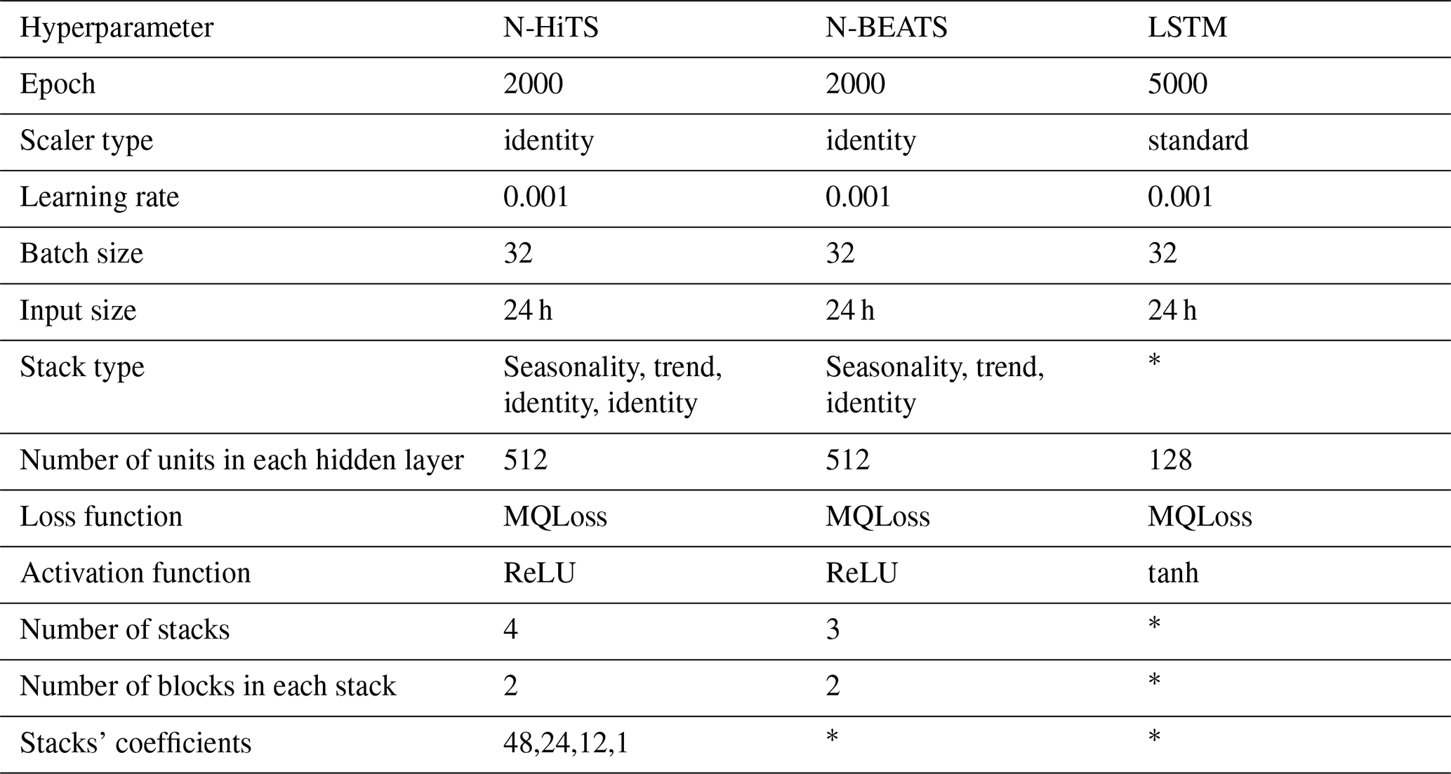
Figure 6 shows the workflow of programming N-BEATS, N-HiTS, and LSTM for flood prediction. As illustrated, the initial step involved cleaning and preparing the input data, which was then used to feed the models. The workflow for each model and their output generation processes are depicted in Fig. 6. We segmented the storm events using the MIT approach, as previously described. Following this, we conducted a sensitivity analysis using the Leave-One-Out method and performed uncertainty analysis using the MLE approach to construct the 95 PPU band. This rigorous methodology ensures a robust evaluation of model performance under varying conditions and highlights the models' predictive reliability and resilience. We employed the “NeuralForecast” Python package to develop the N-BEATS, N-HiTS, and LSTM models. This package provides a diverse array of NN models with an emphasis on usability and robustness.

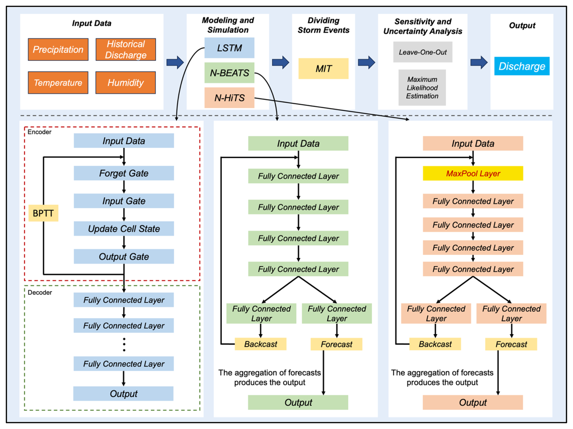
Figure 6 The workflow of N-BEATS, N-HiTS, and LSTM implementation. The upper section of the figure illustrates multiple steps from data preprocessing to model evaluation. The lower section provides a detailed view of the workflow and implementation for each model, highlighting the specific processes and methodologies employed in generating the outputs. Backpropagation Through Time (BPTT) trains LSTM by unrolling the model through time, computing gradients for each time step, and updating weights based on temporal dependencies.

3 Results and Discussion

3.1 Independent Storms Delineation

MIT's contextual delineation of storm events laid the groundwork for in-depth evaluation of rainfall events, enabling isolation and separation of rainfall events that led to significant flooding events. The nuanced outcomes of the MIT assessment contributed significantly to the understanding of rainfall variability and distribution as the dominant contributor to flood generation.

During modeling implementation, the initial imperative was the precise distinction of storm events within the precipitation time series data of each case study. Our findings demonstrate that on average a dry period of 7 h serves as the optimal MIT time for both of our case studies. This outcome signifies that when a dry interval of more than 7 h transpires between two successive rainfall events, these subsequent rainfalls should be considered two distinct storm events. This determination underlines the temporal threshold necessary for distinguishing between individual meteorological phenomena in two case studies.

3.2 Hyperparameter Optimization

In the context of hyperparameter optimization, we systematically considered and tuned various hyperparameters for the N-HiTS, N-BEATS, and LSTM. We searched for learning rates on a log-uniform grid between $\mathrm{1}\times {\mathrm{10}}^{-\mathrm{4}}$ and $\mathrm{1}\times {\mathrm{10}}^{-\mathrm{3}}$, batch sizes $\mathit{\{}\mathrm{16},\mathrm{32},\mathrm{64}\mathit{\}}$, input size $\mathit{\{}\mathrm{1},\mathrm{6},\mathrm{12},\mathrm{24}\mathit{\}}$ h. For the LSTM, recurrent layers $\mathit{\{}\mathrm{1},\mathrm{2},\mathrm{3}\mathit{\}}$, hidden units per layer $\mathit{\{}\mathrm{64},\mathrm{128},\mathrm{256}\mathit{\}}$, activation {tanh,ReLU}, decoder MLP depth $\mathit{\{}\mathrm{1},\mathrm{2},\mathrm{3}\mathit{\}}$, and decoder MLP width $\mathit{\{}\mathrm{64},\mathrm{128},\mathrm{256}\mathit{\}}$ were varied during the simulation run. For N-HiTS, stacks $\mathit{\{}\mathrm{2},\mathrm{3},\mathrm{4}\mathit{\}}$, blocks per stack $\mathit{\{}\mathrm{2},\mathrm{3},\mathrm{4},\mathrm{5}\mathit{\}}$, block MLP width $\mathit{\{}\mathrm{64},\mathrm{128},\mathrm{256}\mathit{\}}$, and block MLP depth $\mathit{\{}\mathrm{2},\mathrm{3},\mathrm{4}\mathit{\}}$ were explored. For N-BEATS, we searched stacks $\mathit{\{}\mathrm{2},\mathrm{3},\mathrm{4}\mathit{\}}$, blocks per stack $\mathit{\{}\mathrm{2},\mathrm{3},\mathrm{4},\mathrm{5}\mathit{\}}$, block MLP width $\mathit{\{}\mathrm{64},\mathrm{128},\mathrm{256}\mathit{\}}$, and block MLP depth $\mathit{\{}\mathrm{2},\mathrm{3},\mathrm{4}\mathit{\}}$; the interpretable (trend/seasonality) basis was kept fixed. Following extensive exploration and fine-tuning of these hyperparameters, the optimal configurations were identified (see Table 2). For the N-HiTS model, the most favorable outcomes were achieved with the following hyperparameter settings: 2000 epochs, “identity” for scaler type, a learning rate of 0.001, a batch size of 32, input size of 24 h, “identity” for stack type, 512 units for hidden layers of each stack, step size of 1, MQLoss as loss function, and “ReLU” for the activation function. As shown in Table 2, the N-HiTS model demonstrated superior performance with 4 stacks, containing 2 blocks each, and corresponding coefficients of 48, 24, 12, and 1, showcasing the significance of these settings for flood prediction.

Table 2 Optimized values for the hyperparameters.

^* Not applicable.

This hyperparameter optimization was also conducted for the N-BEATS model. In this model, we considered 2000 epochs, 3 stacks with 2 blocks, “identity” for scaler type, a learning rate of 0.001, a batch size of 32, input size of 24 h, “identity” for stack type, 512 units for hidden layers of each stack, step size of 1, MQLoss as loss function, and “ReLU” for the activation function.

Moreover, the LSTM as a benchmark model yielded its best results with 5000 epochs, an input size of 24 h, “identity” as the scaler type, a learning rate of 0.001, a batch size of 32, and “tanh” as the activation function. Furthermore, LSTM's hidden state was most effective with two layers containing 128 units, and the MLP decoder thrived with two layers encompassing 128 units. These meticulously optimized hyperparameter settings represent the culmination of efforts to ensure that each model operates at its peak potential, facilitating accurate flood prediction.

In Table 2, “epoch” refers to the number of training steps, and “scaler type” indicates the type of scaler used for normalizing temporal inputs. The “learning rate” specifies the step size at each iteration while optimizing the model, and the “batch size” represents the number of samples processed in one forward and backward pass. The “loss function” quantifies the difference between the predicted outputs and the actual target values, while the “activation function” determines whether a neuron should be activated. The “stacks' coefficients” in the N-HITS model control the frequency specialization for each stack, enabling effective handling of different frequency components in the time series data.

Another hyperparameter for all three models is input size, which is a variable that determines the maximum sequence length for truncated backpropagation during training and the number of autoregressive inputs (lags) that the models considered for prediction. Essentially, input size represents the length of the historical series data used as input to the model. This variable offers flexibility in the models, allowing them to learn from a defined window of past observations, which can range from the entire historical dataset to a subset, tailored to the specific requirements of the prediction task. In the context of flood prediction, determining the appropriate input size is crucial to adequately capture the meteorological data preceding the flood event. To address this, we calculated the time of concentration (TC) of the watershed system and set the input size to exceed this duration. According to the Natural Resources Conservation Service (NRCS, 2010), for typical natural watershed conditions, the TC can be calculated from lag time, the time between peak rainfall and peak discharge, using the formula: $\text{Lag time}=\mathrm{TC}\times \mathrm{0.6}$ (NRCS, 2010). Specifically, the average TC in the Lower Dog River watershed and Upper Dutchmans Creek watershed was found to be 19 and 22 h, respectively. As these represent the average TC for our case studies, we selected the 24 h for input data, slightly longer than the average TC, ensuring sufficient coverage of relevant meteorological data preceding all flood events.

3.3 Flood Prediction and Performance Assessment

In this study, we conducted a comprehensive performance evaluation of N-HiTS, N-BEATS, and benchmarked these models with LSTM, utilizing two case studies: the Lower Dog River and the Upper Dutchmans Creek watersheds. Within these case studies, we trained and validated the models separately for each watershed across a diverse set of storm events from 1 October 2007 to 1 October 2022 (15 years) in the Lower Dog River and from 21 December 1994 to 1 October 2022 (27 years) in the Upper Dutchmans Creek. The decision to train separate models for each catchment was made to account for the unique hydrological characteristics and local features specific to each watershed. By training models individually, we aimed to optimize performance by tailoring each model to the distinct rainfall-runoff relationship inherent in each catchment. All algorithms were tested using unseen flooding events that occurred between 14 December 2022 and 28 March 2023. Our targets were event-focused, where operational value focuses on performance during rising limbs, peaks, and recessions. Evaluating over the entire continuous hydrograph (testing period) can dilute or even mask differences. For this reason, we prioritized an event-centric assessment as the primary evaluation approach rather than full-period metrics. In the Dog River gauging station, two winter storms, i.e., 3 to 5 January 2023 (Event 1) and 17 to 18 February 2023 (Event 2), as well as a spring flood event that occurred during 26 to 28 March 2023 (Event 3) were selected for testing. Additionally, three winter flooding events, i.e., 14 to 16 December 2022 (Event 4), 25 and 26 January 2023 (Event 5), and 11 to 13 February 2023 (Event 6), were chosen to test the algorithms across the Killian Creek gauging station in the Upper Dutchmans Creek. The rainfall events corresponding to these flooding events were delineated using the MIT technique discussed in Sect. 3.1.

Our results for the Lower Dog River case study explicitly demonstrated the accuracy of both N-HiTS and N-BEATS in generating the winter and spring flood hydrographs compared to the LSTM model across all selected storm events. Although, N-HiTS prediction slightly outperformed N-BEATS during winter prediction (3 to 5 January 2023). In this event, N-HiTS outperformed N-BEATS with a difference of 11.6 % in MAE and 20 % in RMSE. The N-HiTS slight outperformance (see Tables 3 and 4) is attributed to its unique structure that allows the model to discern and capture intricate patterns within the data. Specifically, N-HiTS predicted flooding events hierarchically using blocks specialized in different rainfall frequencies based on controlled signal projections, through expressiveness ratios, and interpolation of each block. The coefficients are then used to synthesize backcast through ${\stackrel{\mathrm{̃}}{y}}_t-L:tl$ and forecast (${\stackrel{\mathrm{̃}}{y}}_{t+\mathrm{1}}:t+Hl$) outputs of the block as a flood value. The coefficients were locally determined along the horizon, allowing N-HiTS to reconstruct nonstationary signals over time.

Table 3 The performance metrics for the Lower Dog River flood predictions with 1 h prediction horizon.

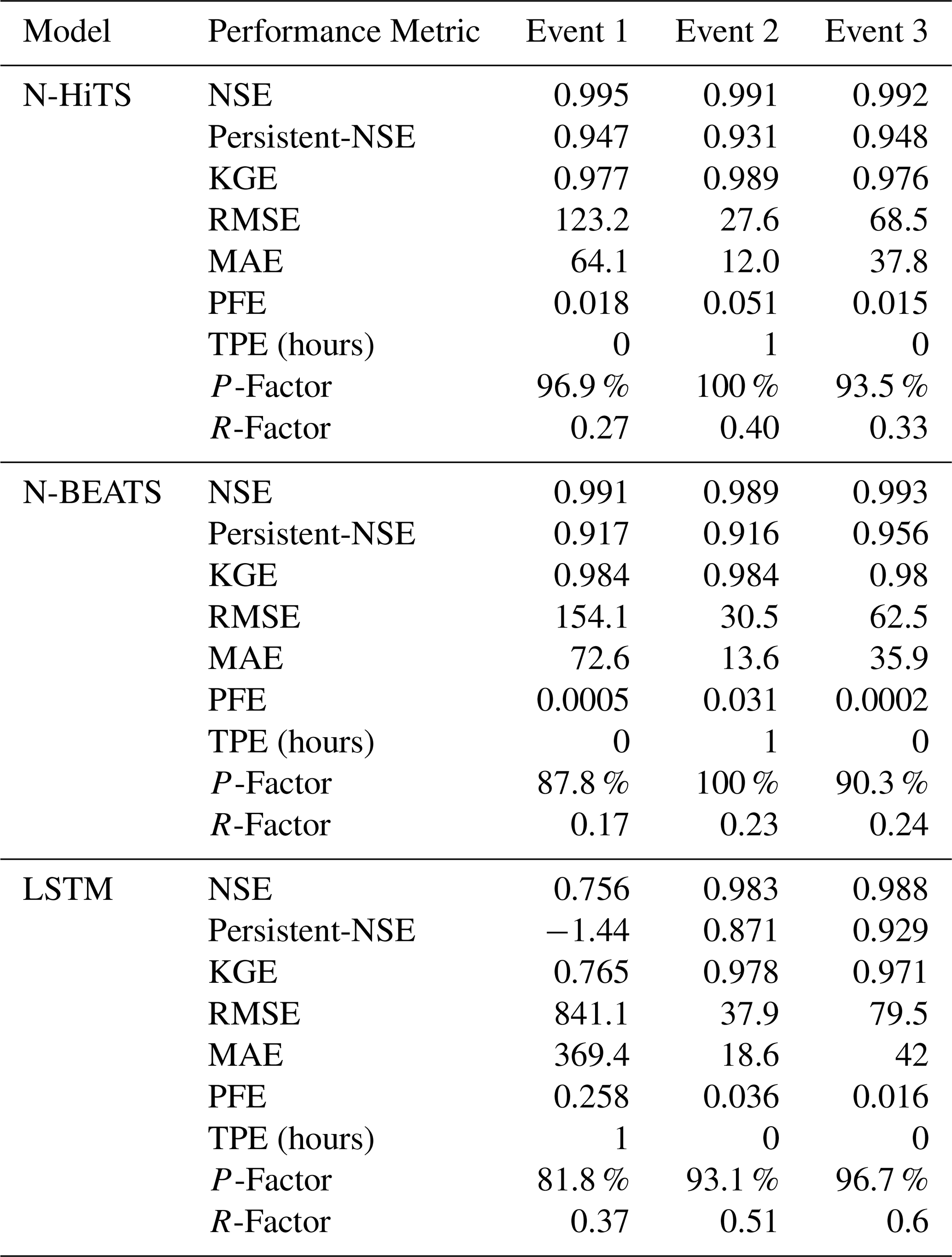
Table 4 The performance metrics for the Killian Creek flood predictions with 1 h prediction horizon.

While the N-HiTS emerged as the most accurate in predicting flood hydrograph among the three models, its performance was somehow comparable with N-BEATS. The N-BEATS model exhibited good performance in two case studies. It consistently provided competitive results, demonstrating its capacity to effectively handle diverse storm events and deliver reliable predictions. N-BEATS has a generic and interpretable architecture depending on the blocks it uses. Interpretable configuration sequentially projects the signal into polynomials and harmonic basis to learn trend and seasonality components while generic configuration substitutes the polynomial and harmonic basis for identity basis and larger network's depth. In this study, we used interpretable architecture, as it regularizes its predictions through projections into harmonic and trend basis that is well-suited for flood prediction tasks. Using interpretable architecture, flood prediction was aggregated in a hierarchical fashion. This enabled the building of a very deep neural network with interpretable flood prediction outputs.

It is essential to underscore that, despite its strong performance, the N-BEATS model did not surpass the N-HiTS model in terms of NSE, Persistent-NSE, MAE, and RMSE for the Lower Dog River case study. Although both models showed almost the same KGE values. Notably, the N-BEATS model showcased superior results based on the PFE metric, signifying its exceptional capability in accurately predicting flood peaks. However, both N-HiTS and N-BEATS models overestimated the flood peak rate of Event 2 for the Lower Dog River watershed. This event, which occurred from 17 to 18 February 2023, was flashy, short, and intense proceeded by a prior small rainfall event (from 12 until 13 February) that minimized the rate of infiltration. This flash flood event caused by excessive rainfall in a short period of time (<8 h) was challenging to predict for N-BEATS and N-HiTS models. In addition, predicting the magnitude of changes in the recession curve of the third event seems to be a challenge for both models. The specific part of the flood hydrograph after the precipitation event, where flood diminishes during a rainless is dominated by the release of runoff from shallow aquifer systems or natural storages. It seems both models showed a slight deficiency in capturing this portion of the hydrograph when the rainfall amount decreases over time in the Dog River gauging station.

Conversely, in the Killian Creek gauging station, the N-BEATS model almost emerged as the top performer in predicting the flood hydrograph based on NSE, Persistent-NSE, RMSE, and PFE performance metrics (see Tables 3 and 4). KGE values remained almost the same for both models. In addition, both N-BEATS and N-HiTS slightly overpredicted time to peak values for Event 5. This reflects the fact that when rainfall varies randomly around zero, it provides less to no information for the algorithms to learn the fluctuations and patterns in time series data. Both N-HiTS and N-BEATS provided comparable results for all events predicted in this study. N-HiTS builds upon N-BEATS by adding a MaxPool layer at each block. Each block consists of an MLP layer that learns how to produce coefficients for the backcast and forecast outputs. This subsamples the time series and allows each stack to focus on either short-term or long-term effects, depending on the pooling kernel size. Then, the partial predictions of each stack are combined using hierarchical interpolation. This ability enhances N-HiTS capabilities to produce drastically improved, interpretable, and computationally efficient long-horizon flood predictions.

In contrast, the performance of LSTM as a benchmark model lagged behind both N-HiTS and N-BEATS models for all events across two case studies. Despite its extensive applications in various hydrology domains, the LSTM model exhibited comparatively lower accuracy when tasked with predicting flood responses during different storm events. Focusing on NSE, Persistent-NSE. KGE, MAE, RMSE, and PFE metrics, it is noteworthy that all three models, across both case studies, consistently succeeded in capturing peak flow rates at the appropriate timing. All models demonstrated commendable results with respect to the TPE metric. In most scenarios, TPE revealed a value of 0, signifying that the models accurately pinpointed the peak flow rate precisely at the expected time. In some instances, TPE reached a value of 1, showing a deviation of one hour in predicting the peak flow time. This deviation is deemed acceptable, particularly considering the utilization of short, intense rainfall for our analysis.

Our investigation into the performance of the three distinct forecasting models yielded compelling results pertaining to their ability to generate 95 PPU, as quantified by the P-Factor and R-Factor. These factors serve as critical indicators for assessing the reliability and precision of the uncertainty bands produced by the MLE. Our findings demonstrated that the N-HiTS and N-BEATS models outperformed the LSTM model in mathematically defining uncertainty bands, in terms of R-Factor metric. The R-Factor, a crucial metric for evaluating the average width of the uncertainty band, consistently favored the N-HiTS and N-BEATS models over their counterparts. This finding was consistent across a diverse range of storm events. In addition, coupling MLE with the N-HiTS and N-BEATS models demonstrated superior performance in generating 95 PPU when assessed through the P-Factor metric. The P-Factor represents another vital aspect of uncertainty quantification, focusing on the precision of the uncertainty bands.

Figures 7 and 8 present graphical depictions of the predicted flood with 1 h prediction horizon and uncertainty assessment for each model as well as Flow Duration Curve (FDC) across two gauging stations.  As illustrated, the uncertainty bands skillfully bracketed most of the observational data, reflecting the fact that MLE was successful in reducing errors in flood prediction. FDC analysis also revealed that N-HiTS and N-BEATS models skillfully predicted the flood hydrograph, however, both models were particularly successful in predicting moderate to high flood events (1800–6000 and >6000 cfs). In the FDC plots, the x-axis denotes the exceedance probability, expressed as a percentage, while the y-axis signifies flood in cubic feet per second. Notably, these plots reveal distinctive patterns in the performance of the N-HiTS, N-BEATS, and LSTM models.

Figure 7 95 PPU band and FDC plots of N-HiTS, N-BEATS, and LSTM models with 1 h prediction horizon for the three selected flooding events in the Lower Dog River gauging station.

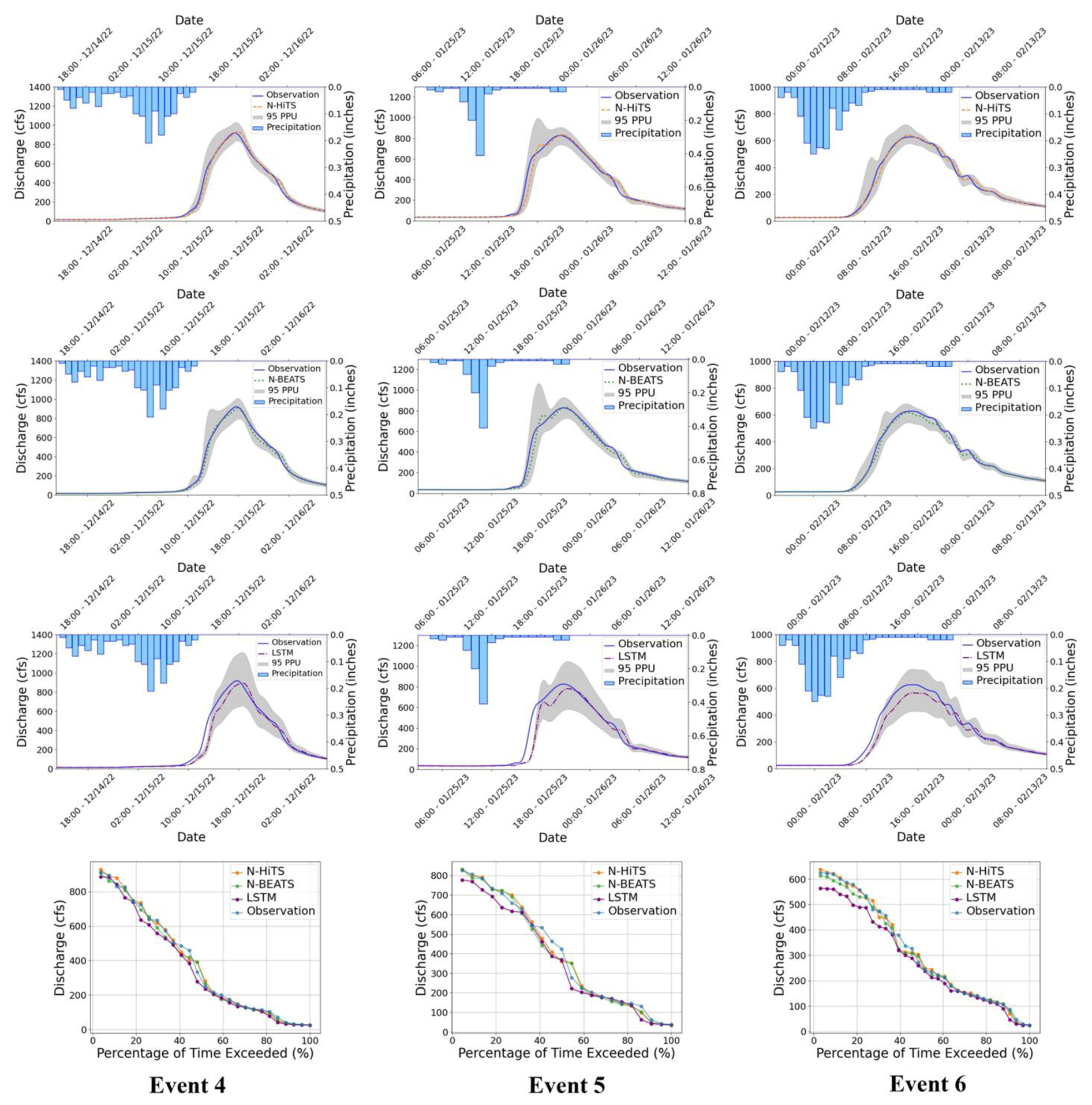
Figure 8 95 PPU band and FDC plots of N-HiTS, N-BEATS, and LSTM models with 1 h prediction horizon for the three selected flooding events in the Killian Creek gauging station.

Within the lower exceedance probability range, particularly around the peak flow, the N-HiTS and N-BEATS models demonstrated a clear superiority over the LSTM model, closely aligning with the observed data. This observed trend is consistent when examining the corresponding hydrographs. Across all events, the flood hydrographs generated by N-HiTS and N-BEATS exhibited a closer resemblance to the observed data, particularly in the vicinity of the peak timing and rate, compared to the hydrographs produced by the LSTM model. These findings underscore the enhanced predictive accuracy and reliability of the N-HiTS and N-BEATS models, particularly in predicting moderate to high flood events as well as critical hydrograph features such as peak flow rate and timing. The alignment of model-generated FDCs and hydrographs with observed data in the proximity of peak flow further establishes the efficiency of N-HiTS and N-BEATS in accurately reproducing the dynamics of flood generation mechanisms across two headwater streams.

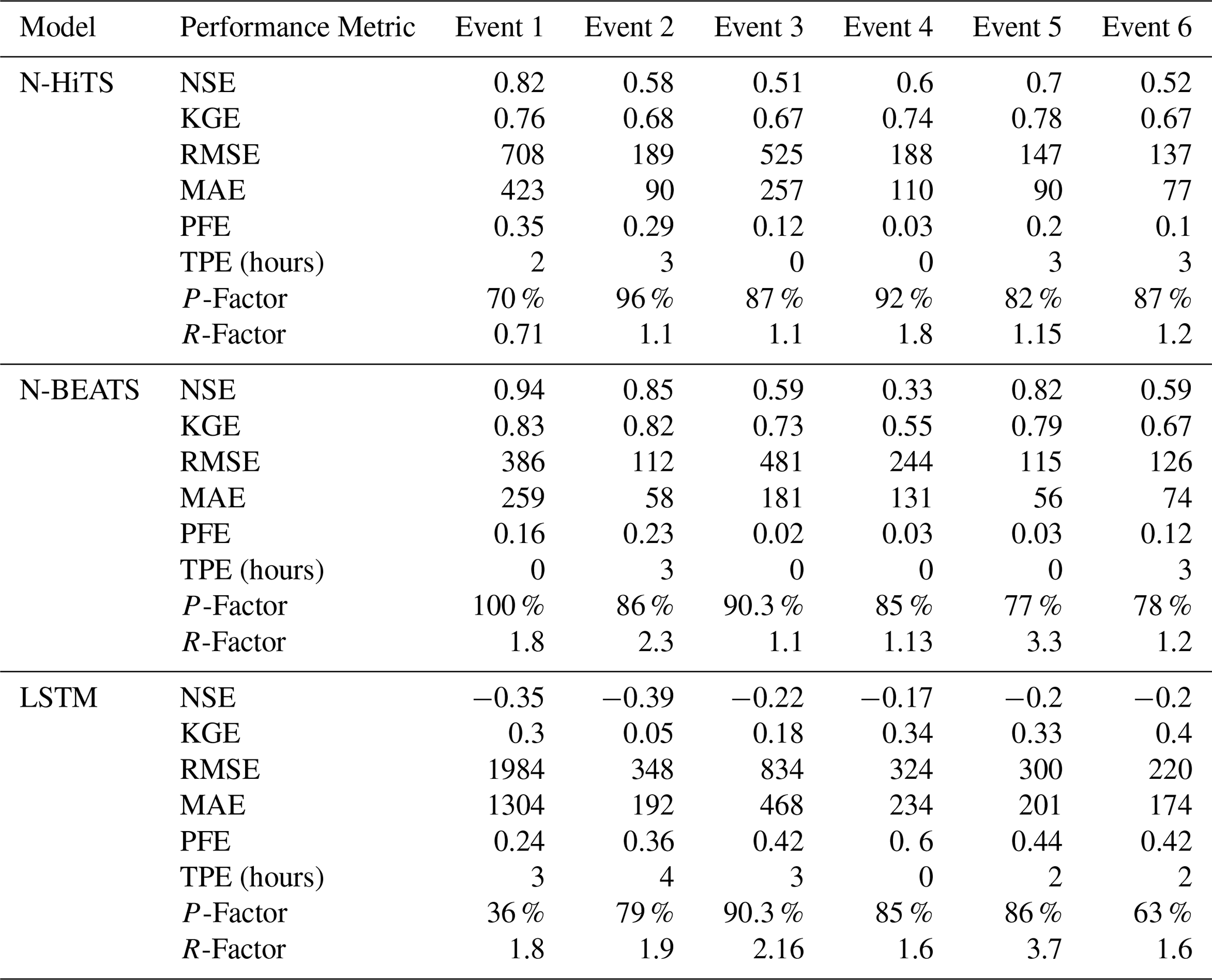
To evaluate robustness across lead times, we extended the analysis to 3 and 6 h prediction horizons. The results are presented in Figs. 9–12, and Tables 5 and 6. As expected, NSE and KGE decreased while the absolute errors increased with horizon for all models; however, N-HiTS and N-BEATS continued to outperform LSTM across both stations and events. At Killian Creek station, both N-HiTS and N-BEATS preserved their lead, yielding higher NSE and lower MAE/RMSE than LSTM, while at the Lower Dog River, N-BEATS remained slightly superior on the same metrics. KGE values stayed comparable between the two feed-forward models, and peak-focused metrics (PFE and TPE) indicated that both still captured peak magnitude and timing reliably, compared to LSTM. Uncertainty bands widened with horizon as expected, but the likelihood-based 95 PPU for N-HiTS and N-BEATS maintained tighter R-Factors and competitive P-Factors relative to LSTM, especially around moderate-to-high flows. Flow-duration diagnostics at multi-hour leads reinforced these findings, showing closer alignment of N-HiTS and N-BEATS to observations in the upper tail. Overall, the multi-horizon results corroborate the 1 h horizon results: N-HiTS and N-BEATS deliver more accurate and reliable flood forecasts than LSTM, and their relative strengths persist at 3 and 6 h ahead. For completeness, we also evaluated 12 and 24 h lead times. During these horizons, all models' performances declined sharply (NSE <0.4 across sites and events), so we restrict detailed reporting to 1–6 h where performance remains operationally meaningful.

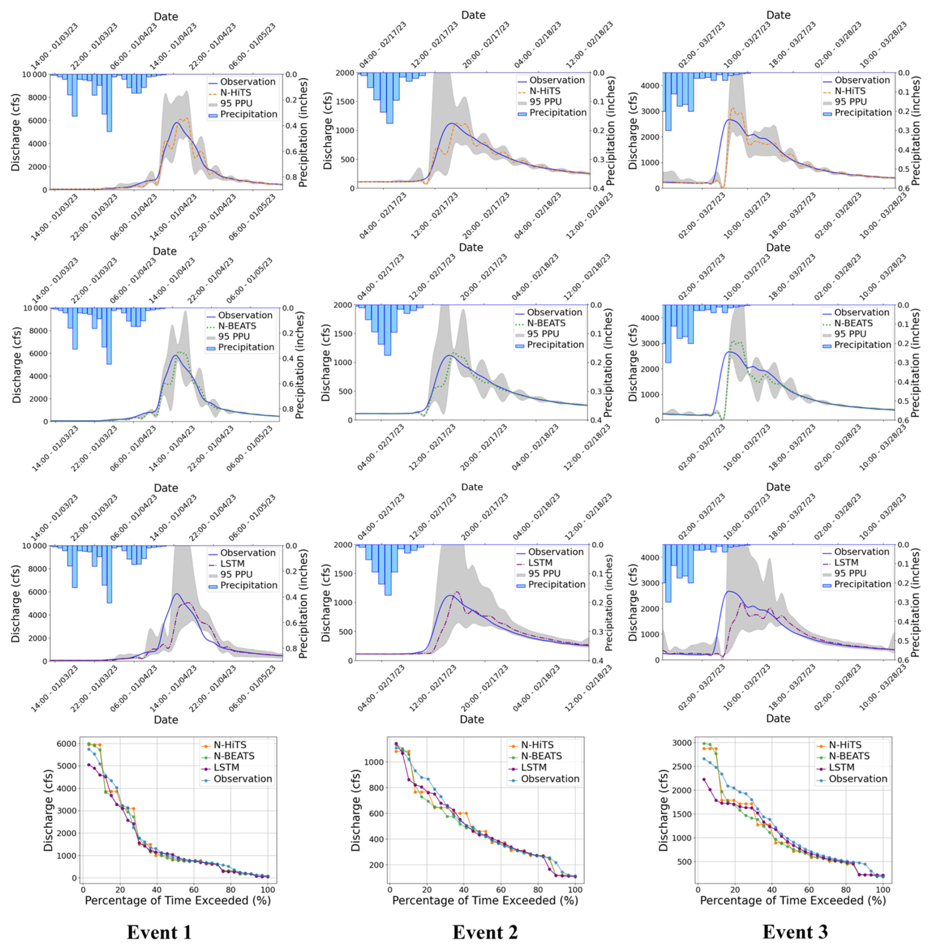
Figure 9 95 PPU band and FDC plots of N-HiTS, N-BEATS, and LSTM models with 3 h prediction horizon for the three selected flooding events in the Lower Dog River gauging station.

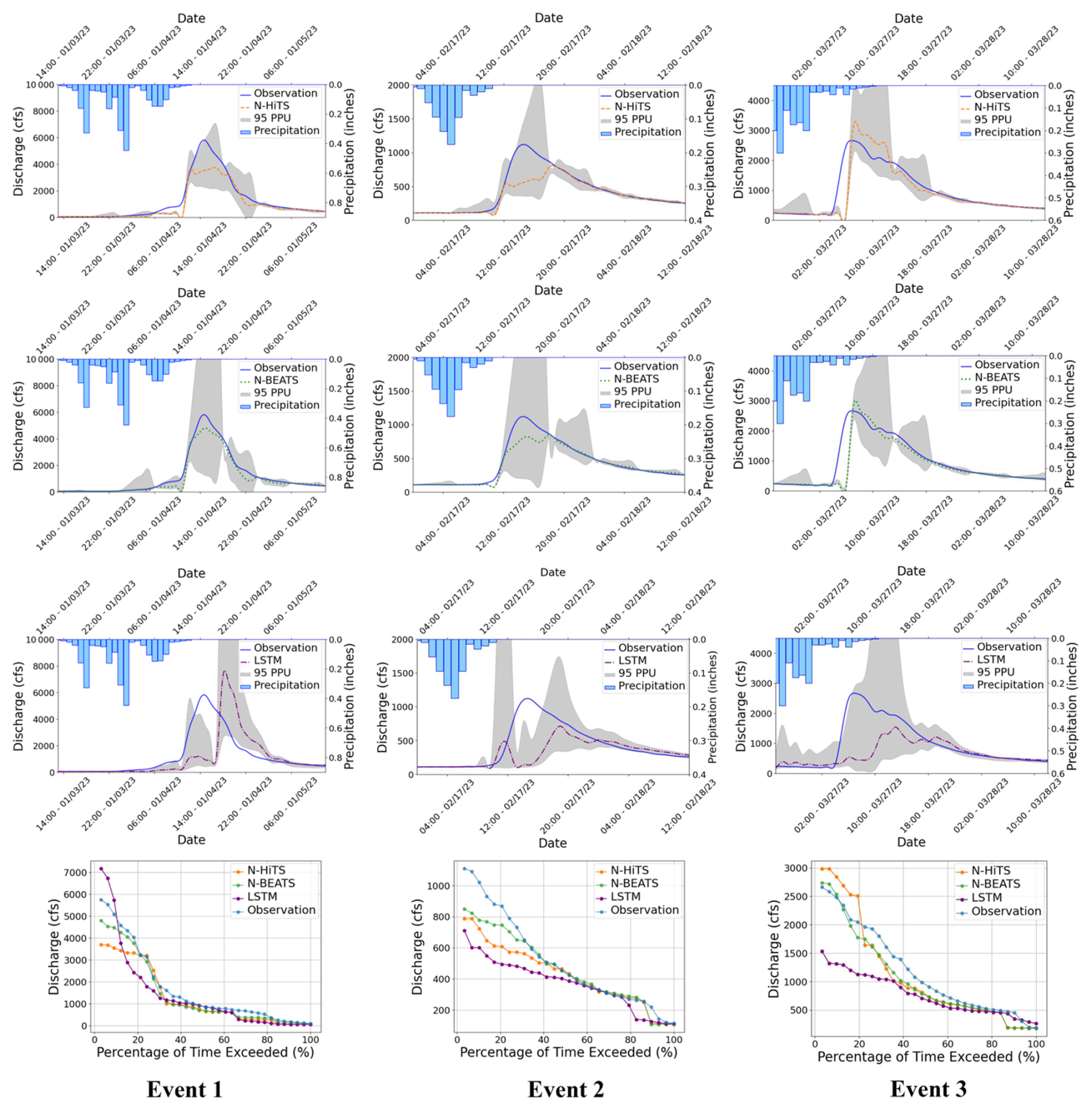
Figure 10 95 PPU band and FDC plots of N-HiTS, N-BEATS, and LSTM models with 6 h prediction horizon for the three selected flooding events in the Lower Dog River gauging station.

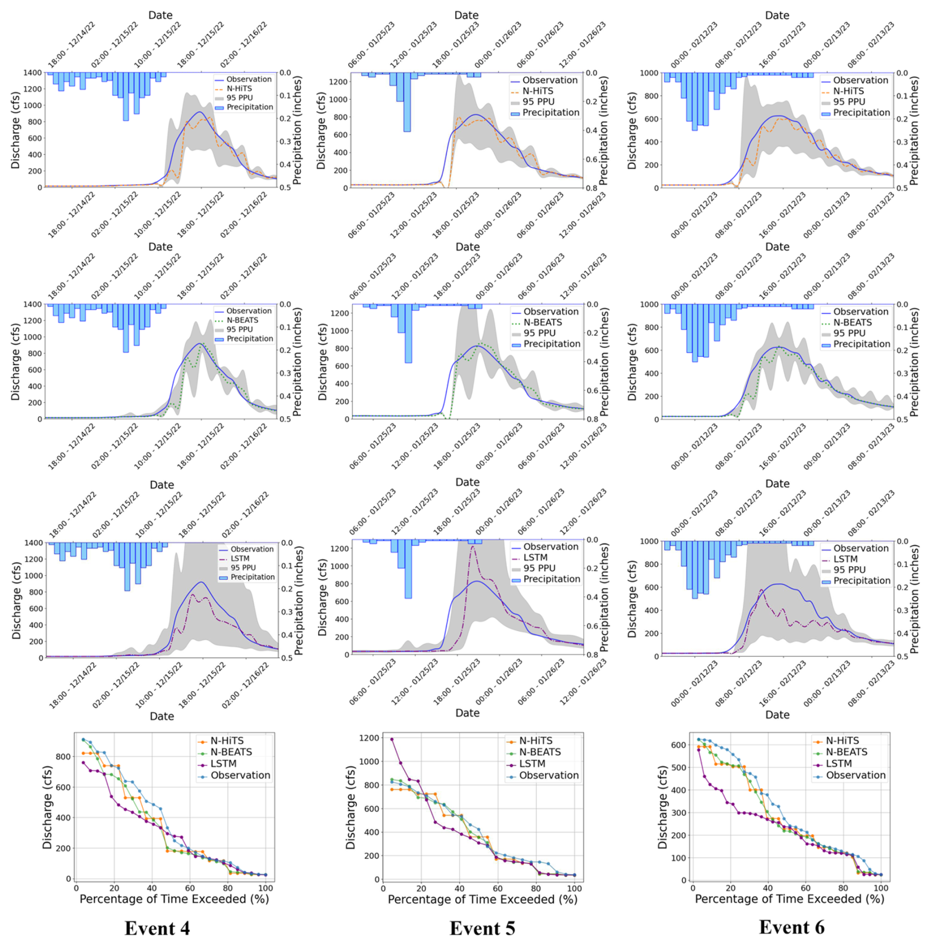
Figure 11 95 PPU band and FDC plots of N-HiTS, N-BEATS, and LSTM models with 3 h prediction horizon for the three selected flooding events in the Killian Creek gauging station.

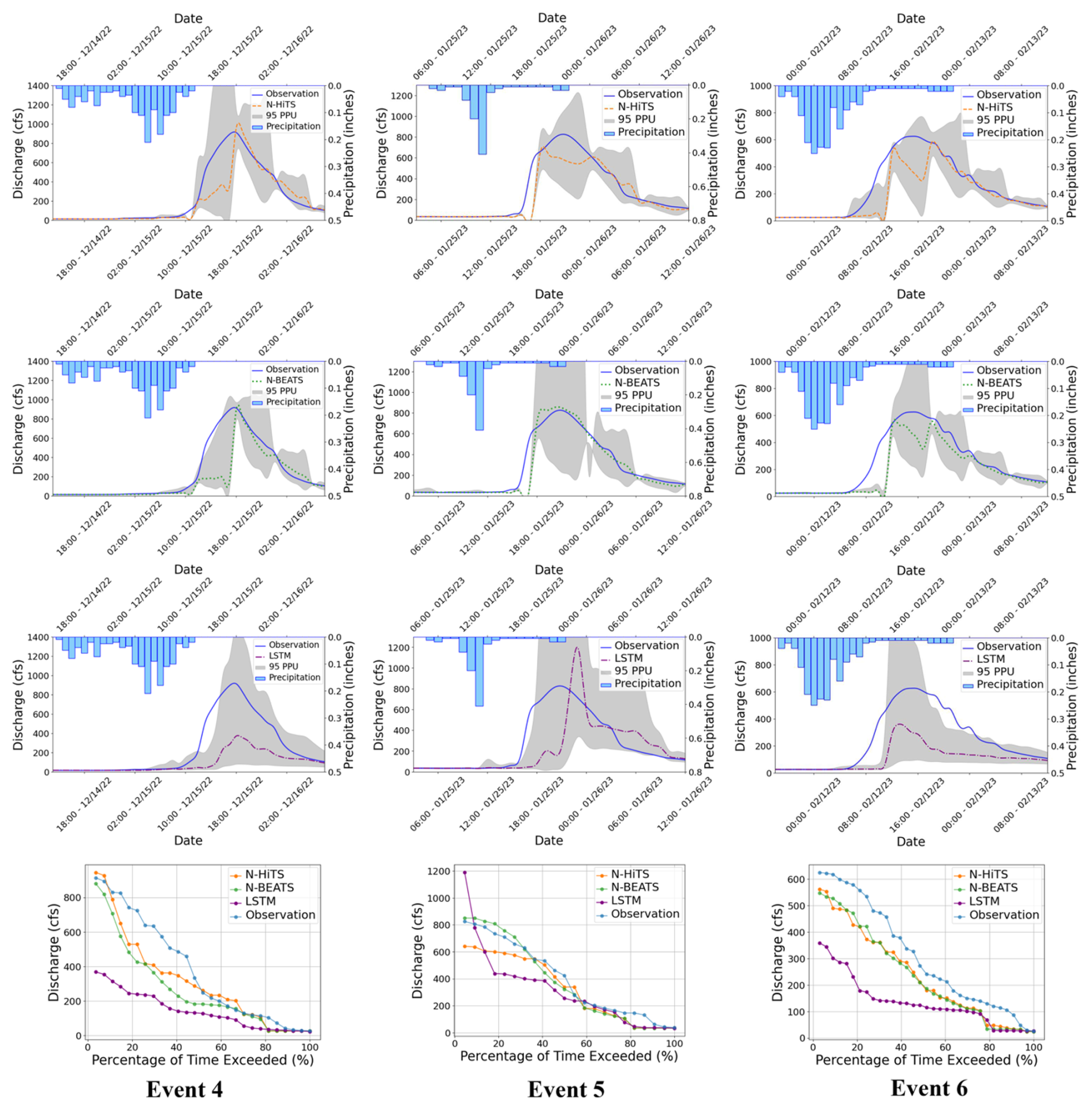
Figure 12 95 PPU band and FDC plots of N-HiTS, N-BEATS, and LSTM models with 6 h prediction horizon for the three selected flooding events in the Killian Creek gauging station.

Table 5 The performance metrics of the models with 3 h prediction horizon.

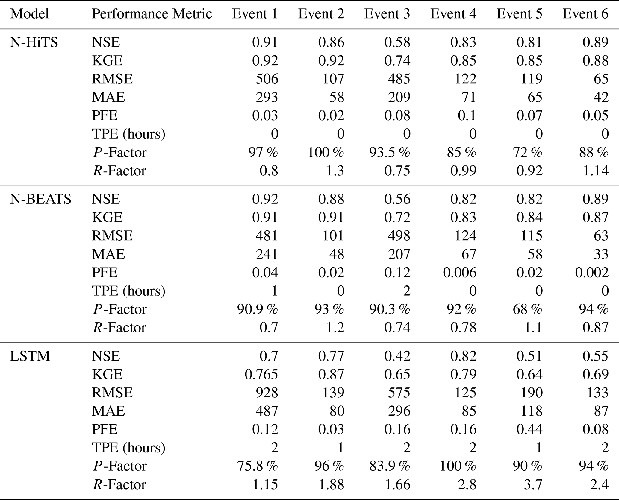
Table 6 The performance metrics of the models with 6 h prediction horizon.

To probe cross-catchment generalizability, we trained a single “regional” model by pooling Lower Dog River and Killian Creek, preserving per-site temporal splits and fitting a global scaler only on the pooled training portion to avoid leakage; evaluation remained strictly per site. Relative to per-site training, pooled fitting produced a small accuracy drop for N-HiTS and N-BEATS (∼ 2 % to 3 %). LSTM showed mixed performance to pooling, it improved in some storm events but degraded in others, so that, when averaged across both stations and storm events, LSTM's regional performance was effectively unchanged relative to the per-site training. Despite that, the regional N-HiTS/N-BEATS matched the accuracy of the best per-site models within the variability observed across storm events and, importantly, consistently surpassed LSTM at both basins. Mechanistically, N-HiTS's multi-rate pooling and hierarchical interpolation, and N-BEATS's trend/seasonality basis projection, act as catchment-invariant feature extractors that support parameter sharing across stations.

In our investigation, we conducted an analysis to assess the impact of varying input sizes on the performance of the N-HiTS, as the best model. We implemented four different durations as input sizes to observe the corresponding differences in modeling performance. Notably, one of the key metrics affected by changes in input size was 95 PPU, which exhibited a general decrease with increasing input size. As detailed in Table 7, we observed a discernible trend in the R-Factor of the N-HiTS model as the input size was increased. Specifically, there was a decline in the R-Factor as the input size expanded. This trend underscores the influence of input size on model performance, particularly in terms of 95 PPU band and accuracy.

Table 7 N-HiTS's R-Factor results for three storm events in each case study, using 1, 6, 12, and 24 h input size in training.

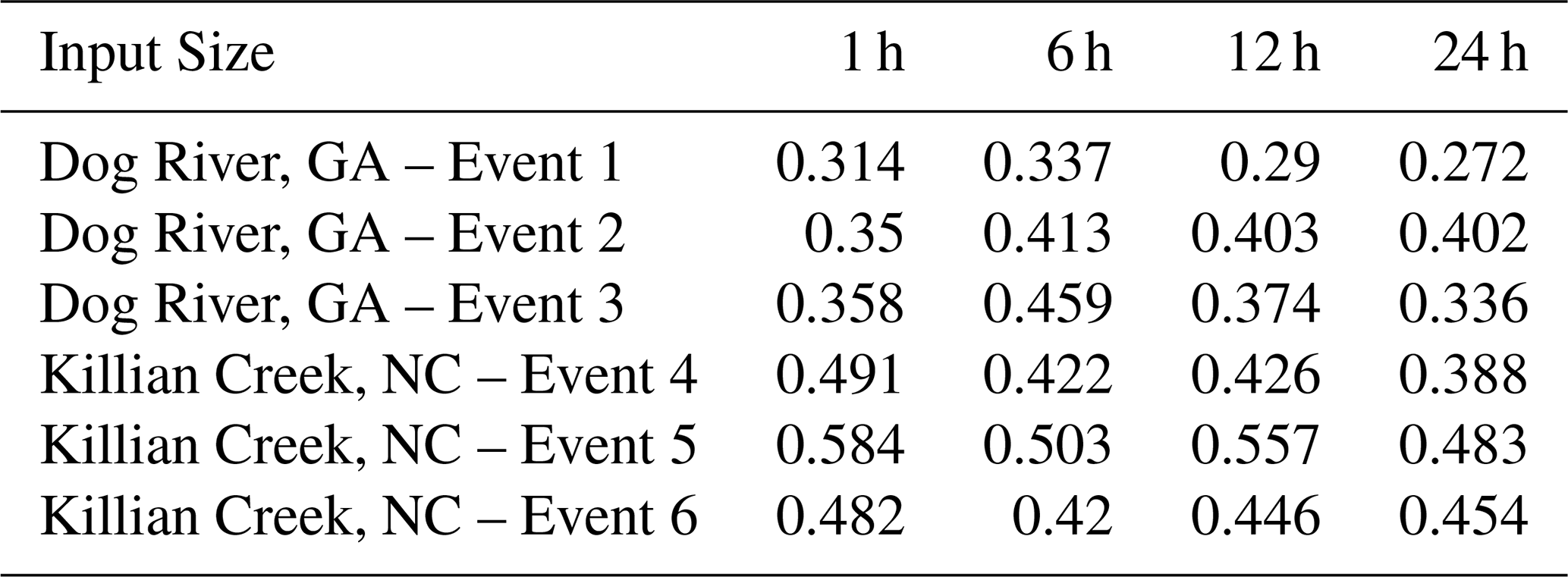
Overall, uncertainty analysis revealed that coupling MLE with N-HiTS and N-BEATS models demonstrated superior performance in generating 95 PPU, effectively reducing errors in flood prediction. The MLE approach was more successful in reducing 95 PPU bands of N-HiTS and N-BEATS models compared to the LSTM, as indicated by the R-Factor and P-Factor. The N-BEATS model demonstrated a narrower uncertainty band (lower R-Factor value), while the N-HiTS model provided higher precision. Furthermore, incorporating data with various sizes into the N-HiTS model led to a narrower 95 PPU and an improvement in the R-Factor, highlighting the significance of input size in enhancing model accuracy and reducing uncertainty.

3.4 Sensitivity Analysis

In this study, we conducted a comprehensive sensitivity analysis of the N-HiTS, N-BEATS, and LSTM models to evaluate their responsiveness to meteorological variables, specifically precipitation, humidity, and temperature. The goal was to assess how the omission of input features impacts the overall modeling performance compared to their full-variable counterparts.

To execute this analysis, we systematically trained each model by excluding meteorological variables one or more at a time, subsequently evaluating their predictive performance using the entire testing dataset. The results of our analysis indicated that N-HiTS and N-BEATS models exhibited minimal sensitivity to meteorological variables, as evidenced by the negligible impact on their performance metric (i.e., NSE, Persistent-NSE, KGE, RMSE, and MAE) upon input feature exclusion.

Notably, as shown in Table 8, the performance of the N-HiTS model displayed a marginal deviation under variable omission, while the N-BEATS model exhibited consistent performance irrespective of the inclusion or exclusion of meteorological variables. The structure of this algorithm is based on backward and forward residual links for univariate time series point forecasting which does not take into account other input features in the prediction task.  These findings suggest that the predictive capabilities of N-HiTS and N-BEATS models predominantly rely on historical flood data. Both models demonstrated strong performance even without incorporating precipitation, temperature, or humidity data, underscoring their ability in flood prediction in the absence of specific meteorological inputs. This capability underscores the robustness of the N-HiTS and N-BEATS models, positioning them as viable tools and perhaps appropriate for real-time flood forecasting tasks where direct meteorological data may be limited or unavailable.

Table 8 Performance metrics' values for N-HiTS, N-BEATS, and LSTM models by excluding meteorological variables one or more at a time.

3.5 Computational Efficiency

The computational efficiency of the N-HiTS, N-BEATS, and LSTM models, as well as a comparative analysis, is presented in Table 9. The study encompassed the entire process of training and predicting over the testing period, employing the optimized hyperparameters as previously described. Regarding the training time, it is noteworthy that the LSTM model exhibited the quickest performance. Specifically, LSTM demonstrated a training time that was 71 % faster than N-HiTS and 93 % faster than N-BEATS in the Lower Dog River watershed, while it was respectively,126 % and 118 % faster than N-HiTS and N-BEATS in the Upper Dutchmans Creek, over training dataset. This is because LSTM has simple architecture compared to the N-BEATS and N-HiTS and does not require multivariate features, hierarchical interpolation, and multi-rate data sampling. Perhaps, this outcome underscores the computational advantage of LSTM over other algorithms.

Table 9 Computational costs of N-HiTS, N-BEATS, and LSTM models in the Dog River and Killian Creek gauging stations.

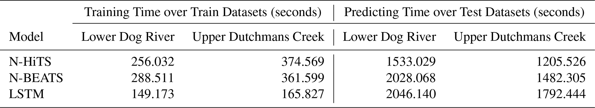
Conversely, during the testing period, the N-HiTS model emerged as the fastest and delivered the most efficient results in comparison to the other models. Notably, N-HiTS displayed a predicted time that was 33 % faster than LSTM and 32 % faster than N-BEATS. This finding highlights the computational efficiency of the N-HiTS model in the context of predicting processes. Our experiments unveiled an interesting contrast in the computational performance of these models. While LSTM excelled in terms of training time, it lagged behind when it came to the testing period.

In the grand scheme of computational efficiency, model accuracy, and uncertainty analysis results, it becomes evident that the superiority of the N-HiTS and N-BEATS models in terms of accuracy and uncertainty analysis holds paramount importance. This significance is accentuated by the critical nature of flood prediction, where precision and certainty are pivotal. Therefore, computational efficiency must be viewed in the context of the broader objectives, with the accuracy and reliability of flood predictions taking precedence in ensuring the safety and preparedness of the affected regions.

4 Conclusions

This study examined multiple NN algorithms for flood prediction. We selected two headwater streams with minimal human impacts to understand how NN approaches can capture flood magnitude and timing for these natural systems. In conclusion, our study represents a pioneering effort in exploring and advancing the application of NN algorithms, specifically the N-HiTS and N-BEATS models, in the field of flood prediction. In our case studies, both N-HiTS and N-BEATS models achieved state-of-the-art results, outperforming LSTM as a benchmark model, particularly in one-hour prediction. While a one-hour lead time may seem brief, it is highly significant for accurate flash flood prediction particularly in an area with a proximity to metropolitan cities, where rapid response is critical. These benchmarking results are arguably a pivotal part of this research. However, the N-BEATS model slightly emerged as a powerful and interpretable tool for flood prediction in most selected events.

This study focused on short-lead, operational forecasting at gauged sites, using historical discharge to deliver robust, low-latency updates. While the evaluation is limited to two Southeastern U.S. basins, the architecture (e.g., N-HiTS) is flexible and can incorporate additional covariates and catchment attributes. Extending the approach to ungauged or other basins is feasible through multi-basin training and transfer learning or few-shot adaptation when even brief warm-up records are available. These extensions represent promising directions for future work to assess geographic transferability under the same operational assumptions.

In addition, the results of the experiments described above demonstrated that N-HiTS multi-rate input sampling and hierarchical interpolation along with N-BEATS interpretable configuration are effective in learning location-specific runoff generation behaviors. Both algorithms with an MLP-based deep neural architecture with backward and forward residual links can sequentially project the data signal into polynomials and harmonic basis needed to predict intense storm behaviors with varied magnitudes. The innovation in this study, besides benchmarking the LSTM model for headwater streams, was to tackle volatility and memory complexity challenges, by locally specializing flood sequential predictions into the data signal's frequencies with interpretability, and hierarchical interpolation and pooling. Both N-HiTS and N-BEATS models offered similar performance as compared with the LSTM but also offered a level of interpretability about how the model learns to differentiate aspects of complex watershed-specific behaviors via data. The interpretability of N-HiTS and N-BEATS arises directly from their model architecture.

In the interpretable N-BEATS framework, forecasts are decomposed into trend and seasonality stacks, each represented by explicit basis coefficients that reveal how different temporal patterns contribute to the prediction. Similarly, N-HiTS achieves interpretability by aggregating contributions across multiple distinct time scales, allowing insight into the temporal dynamics driving each forecast. N-HiTS aims to enhance the accuracy of long-term time-series forecasts through hierarchical interpolation and multi-scale data sampling, allowing it to focus on different data patterns, which prioritizes features essential to understand flood magnitudes. N-BEATS leverages interpretable configurations with trend and seasonality projections, enabling it to decompose time series data into intuitive components. N-BEATS interpretable architecture is recommended for scarce data settings (such as flooding event), as it regularizes its predictions through projections onto harmonic and trend basis.

These approaches improve model transparency by allowing understanding of how each part of the model contributes to the final prediction, particularly when applied to complex flood patterns. Both models also support multivariate series (and covariates) by flattening the model inputs to a 1-D series and reshaping the outputs to a tensor of appropriate dimensions. This approach provides flexibility to handle arbitrary numbers of features. Like LSTM, both N-HiTS and N-BEATS models support producing probabilistic predictions by specifying a likelihood objective. In terms of sensitivity analysis, both N-HiTS and N-BEATS maintain consistent performance even when trained without specific meteorological input.

Although, during some flashy floods, the models encountered challenges in capturing the peak flows and the dynamics of the recession curve, which is directly related to groundwater contribution to flood hydrograph, both models were technically insensitive to rainfall data as an input variable. This suggests the fact that both algorithms can learn patterns in discharge data without requiring meteorological input. This ability underscores these models' robustness in generating accurate predictions using historical flood data alone, making them valuable tools for flood prediction, especially in data-poor watersheds or even for real-time flood prediction when near real-time meteorological inputs are limited or unavailable. In terms of computational efficiency, both N-HiTS and N-BEATS are trained almost at the same pace; however, N-HiTS predicted the test data much quicker than N-BEATS. Unlike N-HiTS and N-BEATS, LSTM excelled in reducing training time due to its simplicity and limited number of parameters.

Moving forward, it is worth mentioning that predicting the magnitude of the recession curve of flood hydrographs was particularly challenging for all models. We argue that this is because the relation between base flow and time is particularly hard to calibrate due to ground-water effluent that is controlled by geological and physical conditions (vegetation, wetlands, and wet meadows) in headwater streams. In addition, the situations of runoff occurrence are diverse and have a high measurement variance with high frequency that can make it difficult for the algorithms to fully capture discrete representation learning on time series.

In future studies, it will be important to develop strategies to derive analogs to the interpretable configuration as well as multi-rate input sampling, hierarchical interpolation, and backcast residual connections that allow for the dynamic representation of flood times series data with different frequencies and nonlinearity. A dynamic representation of flood time series is, at least in principle, possible by generating additive predictions in different bands of the time-series signals, reducing memory footprint and compute time, and improving architecture parsimony and accuracy. This would allow the model to “learn” interpretability and hierarchical representations from raw data to reduce complexity as the information flows through the network.

While a single station provides valuable localized information, particularly for small, headwater streams where runoff closely follows immediate meteorological conditions, it may not capture the spatial heterogeneity of larger watersheds. In our study, the applied methods successfully captured runoff magnitude and dynamics in small basins for an operational setting. However, broader spatial coverage and distributed data would likely enhance model accuracy for larger regions. Consequently, our conclusions are specifically scoped to the selected basins and forecast horizons, and broader generalizations would require multi-region investigations in future work.

Finally, the performance of N-HiTS, N-BEATS, or other neural network architectures could be further enhanced with robust uncertainty quantification. Approaches such as Bayesian Model Averaging (BMA) with fixed or flexible priors (Samadi et al., 2020) or Markov Chain Monte Carlo (MCMC) optimization methods (Duane et al., 1987) could capture both aleatoric and epistemic uncertainties. We leave these strategies for future exploration in the context of neural flood time-series prediction.