Do convection-permitting regional climate models have added value for hydroclimatic simulations? A test case over small and medium-sized catchments in Germany

Through fine grid structure and explicit representation of deep convective processes, convection-permitting regional climate models (CPRCMs) bear great potential for improved assessment of climate and hydrology under current and future climatic conditions. For a robust assessment of the added value of CPRCMs as climate service for hydrological impact modelling, the current scope of research needs to be expanded by studies on further model structures and study areas. The paper presented here considers the non-hydrostatic model ICON-CLM 2.6.4 at 3 km resolution (ICON3km) and its driving model ICON-CLM 2.6.4 with parametrised convection at 12 km (ICON12km) for a study area of 13 210 km² in East Central Germany, enclosing the small (107 km²) to medium-sized (529 km²) catchments of the upper and central part of the predominantly rural Weiße Elster river basin. The reanalysis-driven historical hourly air temperature, global radiation, relative humidity, wind speed and precipitation simulations are evaluated. ICON3km is further analysed for added value for discharge, soil moisture and evapotranspiration simulation using the distributed hydrological model WaSiM. Our results suggest primarily an improvement by ICON3km in the estimation of air temperature and summer global radiation, as well as a reduction of the overestimation of the left tail of the frequency distribution of wind speed. The most noticeable deficiencies of ICON3km are the strong overestimation of high precipitation intensity and too frequent heavy rainfall events. These shortcomings translate into a pronounced overestimation of discharge when uncorrected, dominating the hydrological impact estimations. As such, no added value in the use of ICON3km for hydrological impact modelling in the Weiße Elster basin was identified.

1 Introduction

Extreme rainfall events around the world are expected to become more intense and more frequent under global warming (IPCC, 2021; Myhre et al., 2019). In the UK for example, the frequency of rainfall events exceeding 20 mm h⁻¹, and thereby capable of producing flash floods, is estimated to be 4-fold by 2070 under a high emission scenario (Kendon et al., 2023). With urbanisation on the rise worldwide (Jiang and O'Neill, 2017) and a growth in population in flood-prone areas (Kam et al., 2021), an increase in the frequency and intensity of local extreme rainfall events leads to large flood risks. Convection-permitting regional climate models (CPRCMs) bear great potential for improved projections of changes in extreme rainfall. These models operate on spatial resolutions smaller than 4 km (Prein et al., 2021) and are built with a non-hydrostatic dynamical core, since the hydrostatic approximation is no longer valid at this scale (Giorgi, 2019; Steppeler et al., 2003). As such, they resolve deep convection and no longer rely on its parametrisation, thereby circumventing a major source of uncertainty (Prein et al., 2015). However, finer scale processes, such as cloud and precipitation microphysics, shallow convection, radiative transfer, and turbulence still need to be parametrised (Prein et al., 2015; Kendon et al., 2021). A full depiction of all energetic processes in clouds would require a downscaling to the smallest scale, i.e. the Kolmogorov scale, where viscous dissipation converts turbulent kinetic energy into heat (Prein et al., 2015; Friedlander and Topper, 1961 cited in Schulz and Sanderson, 2004). Besides a more process-based representation of atmospheric processes, CPRCMs also introduce finer grid spacing, allowing to better capture complex topography and land surface heterogeneities (Gutowski et al., 2020), constituting an added value for impact modelling over small catchments of mountainous or highly urban character (e.g. Schaller et al., 2020; Tamm et al., 2023).

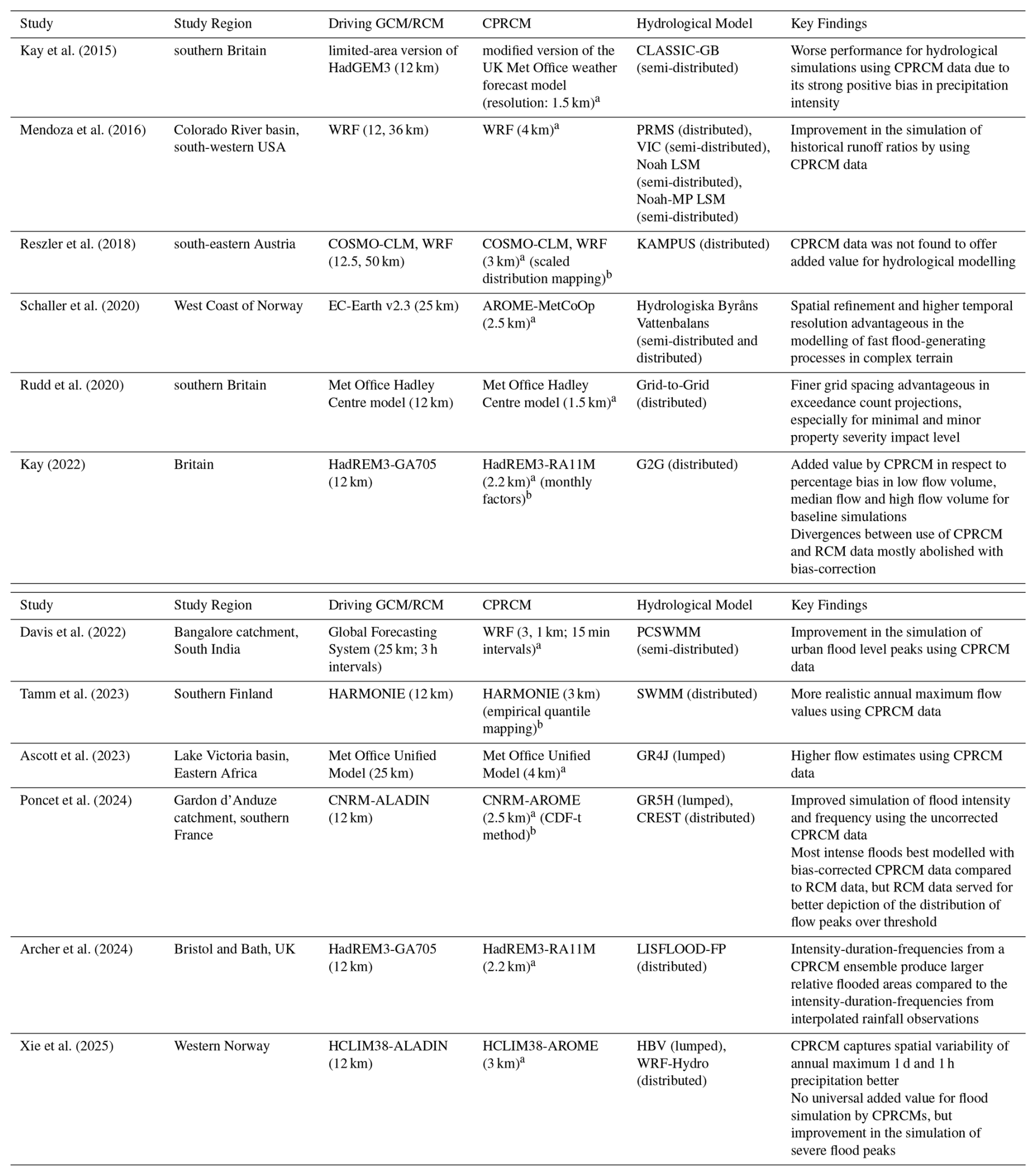
To justify their high computational costs and data storage requirements (Schär et al., 2020), CPRCMs must prove to indeed offer substantial improvement compared to coarser regional climate models with parametrised convection (RCMs). However, in the field of hydrological impact assessment, to this day only a limited number of studies comparing the use of CPRCMs to RCMs have been conducted. An overview is given in Table 1, reflecting how from a state of unsatisfactory performance for impact modelling in the early stages of development (e.g. Kay et al., 2015; Reszler et al., 2018), CPRCMs have made remarkable progress, with a number of recent studies showing substantial added value of CPRCMs for flood simulation. However, with most studies only focusing on a single basin, using data from a single CPRCM, over a short simulation time, there remains an urgent need for further studies (Lucas-Picher et al., 2021). Our paper introduces an additional geographical region and CPRCM to the discourse. It looks at the strengths and limitations of ICON-CLM (2.6.4) in convection-permitting setup at 3 km resolution in depicting hourly near-surface air temperature and relative humidity, wind speed at 10 m, global radiation and precipitation over a chosen catchment in East Central Germany, compared to its driving coarser RCM, ICON-CLM (2.6.4) at 12 km resolution. The focus of the added value of CPRCMs is on the depiction of summer convective events. The climate model data is further used as input to the distributed hydrological model WaSiM to identify potential added value of the studied CPRCM data for discharge simulations in the catchment, while underlining the results by analyses of soil moisture and evapotranspiration estimations.

Table 1 Previous studies investigating the added value of CPRCMs compared to RCMs, with non-bias-corrected (^a) and bias-corrected (^b) precipitation data, for hydrological impact modelling (exclusively model chains consisting of a climate or numerical weather prediction model and a hydrological model are considered).

In this paper, Sect. 2 outlines the study area considered in this paper, the observational and climate model data used, as well as the applied methodology. The results from the meteorological and hydrological data analysis are presented in Sect. 3, while Sect. 4 provides a discussion. A conclusion is given in Sect. 5.

2 Methods and Data

2.1 Study Area

The study area was chosen to encompass the focus regions of the KlimaKonform project (Zorn et al., 2024) in East Central Germany (Fig. 1a). It spans 13 210 km² and hosts the upper and central part of the Weiße Elster river basin (Fig. 1b). The twelve enclosed catchments stretch over an area of 2960 km², with the smallest having an area of 107 km² (Dröda) and the largest of 529 km² (Strassberg).

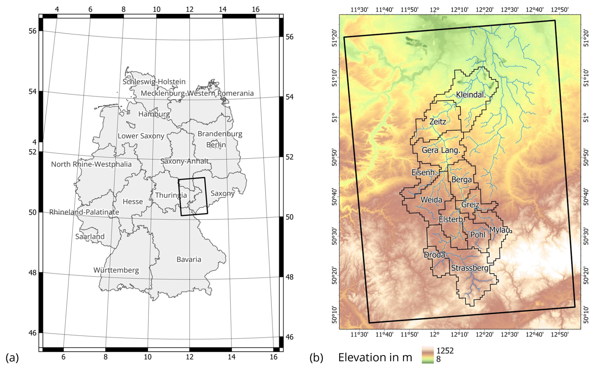
Figure 1 (a) Location of the study area in Germany and (b) the studied catchments within the area over a digital elevation model of 30 m resolution (SRTM 1 arcsec global; USGS, 2018).

The study area is embedded between the Leipzig lowlands to the North and the Elster Mountains and Ore Mountains to the South, resulting in a topographically varied landscape encompassing both flat plains and steeply sloped terrain (Rode et al., 2008; Miera et al., 2022). Altitudes range from 8 to 1252 m on a 30 m grid, from 85 to 1006 m on a 3 km grid, and from 101 to 852 m on a 12 km grid.

The northern part of the study area falls under the Köppen climate classification of Cfb (temperate, no dry season, warm summer), and the southern part is classified as Dfb (cold, no dry season, warm summer). In the study region, floods occur primarily in summer as a result of high-intensity convective storms, as well as in winter due to prolonged rainfall, sometimes amplified by rapid snowmelt.

The land use in the Weiße Elster river basin is predominantly cropland and pasture (Rode et al., 2008, see Fig. S1 in the Supplement). Chernozem/phaeozem and luvisol soils on loess are prevalent in the northern part of the study area, while cambisols and stagnic gleysols dominate the southern part (Miera et al., 2022).

2.2 Observational Data

Hourly observational data from 20 stations for mean air temperature, two stations for global radiation, 20 stations for relative humidity at 2 m, and 11 stations for wind speed at 10 m has been obtained from the German Weather Service (DWD) for the period from 2005 to 2014 (Fig. S2). No spatial interpolation has been performed; the station measurements are compared point-based to the corresponding climate model grid cells. For the assessment of precipitation anomalies, 60-year time series of monthly point-based precipitation data (1963–2022) have been obtained from DWD for five stations in the study area.

For other evaluations of precipitation simulations and hydrological modelling, adjusted radar-based quantitative precipitation estimations are used as reference for the study period from 2005 to 2014 in hourly time steps at a resolution of 1 km. The data set constitutes a gap-filled version of DWD's RADOLAN product (Weigl and Winterrath, 2010) and is provided through the ReKIS portal (Körner, 2022) for the federal states of Saxony, Saxony-Anhalt and Thuringia. RADOLAN is a radar-based precipitation dataset at 1 km resolution, which has been adjusted with measurements from DWD's ground station network (Winterrath et al., 2012). The choice of adjustment procedure is determined based on a performance test with a few control stations (Winterrath et al., 2012). It is unknown whether any, respectively which of these control stations correspond precisely to the stations used in this study. However, the station values can generally be assumed to be preserved.

The data has been upscaled and regridded to the climate model grids using the area-weighted average method (becoming RADOLAN3km and RADOLAN12km). Kreklow et al. (2020) evaluated the performance of the original RADOLAN dataset against rain gauge data and found RADOLAN to overestimate the number of days with daily precipitation sums >1 mm, as well as heavy rainfall days (i.e. daily precipitation sums >20 mm), in the summer half-year. Especially up to the year 2010, extreme high outliers in the time series were not uncommon, with markable improvements through the introduction of additional gauges in 2007, as well as further quality checks and new processing routines in 2010 (Kreklow et al., 2020). However, the average daily precipitation sum for the summer half-year was underestimated, with a similar trend reported for the winter half-year, yet far less pronounced (Kreklow et al., 2020). The mean median of the absolute daily deviations, when comparing RADOLAN data to daily point-based measurements of precipitation for the period from 2013 to 2016, was quantified as 0.761 mm d⁻¹ (DWD, 2021).

The hydrological model was calibrated and validated using Thiessen-interpolated point-based meteorological observations, including hourly precipitation from 20 precipitation gauges in the catchment (see Fig. S2 for a map of the observational network). An evaluation of how the RADOLAN product compares to the Thiessen-interpolated point-based precipitation measurements over the study area is outlined in Fig. S3 by means of a Q–Q plot.

Discharge data along the Weiße Elster has been obtained through the ReKIS project (Kronenberg et al., 2021), based on measurements by the Sächsisches Landesamt für Umwelt, Landwirtschaft und Geologie (LfULG), Thüringer Landesamt für Umwelt, Bergbau und Naturschutz (TLUBN) and Landesamt für Umweltschutz Sachsen-Anhalt (LAU).

Topographic information was obtained from SRTM 1 arcsec global (USGS, 2018), land use is based on Corine Land Cover 2018 (Copernicus Land Monitoring Service, 2020) and used soil data refers to BÜK200 (BGR and SGD, 2018).

2.3 Climate Model Data

The regional climate model ICON-CLM (version 2.6.4, Pham et al., 2021) has been run over the EURO-CORDEX domain at 12 km resolution for hourly output (ICON12km). It is driven three-hourly with data from the global atmospheric reanalysis ECMWF-ERA5 and provides the lateral boundary conditions for the CPRCM. As CPRCM, ICON-CLM (version 2.6.4) is employed in its convection-permitting setup at 3 km resolution over the Central European (CEU) domain providing hourly weather data (ICON3km). The domains are illustrated in Fig. S4. Information on the model dynamics is provided by Zängl et al. (2015).

In ICON12km, deep, mid-level, and shallow convection have been parametrised using the Tietke/Bechtold scheme (Tiedtke, 1989; Bechtold et al., 2008). ICON3km, in turn, operates on a resolution fine enough to explicitly resolve deep and mid-level convection, with only the shallow convection parametrisation needing to remain switched on. Vertical turbulent transfer is parametrised according to Raschendorfer (2008), and cloud microphysics are calculated with the single-moment scheme of Seifert (2008).

Tracer transport and fast-physics parametrisations are computed at time steps of 25 s, while the dynamical core runs at 5 s.

2.4 Evaluation of Simulated Meteorological Data

Air temperature, global radiation, relative humidity, and wind speed station measurements within the catchment bounding box (see Fig. S2) are compared to their co-located climate model grid cells. Air temperature estimates by the climate models are projected to the elevation of the measurement stations using the environmental lapse rate, which is of 0.65 °C/100 m. Precipitation simulations for the area are evaluated raster-based against radar precipitation estimations upscaled and regridded to the climate models' grids. Comparing precipitation simulations to observations on the same grid circumvents the need to consider differences in the degree of smoothing of local heavy rainfall fields with resolution (Iles et al., 2020). While the radar precipitation estimations are upscaled to the resolution of the climate models for comparison between the climate model simulations and the observations, the climate models themselves are not compared among each other by scaling the simulations to a common grid spacing. In fact, upscaling the finer climate simulation results to the grid of the coarser climate model would entail partial information loss (Iles et al., 2020), while downscaling the coarser climate model simulations would bring them into resolutions where processes dominate which are on a scale too fine to have been computed by the coarser model (Prein et al., 2016). It is however worth noting that first studies suggest that improvements at higher resolution may still be apparent after upscaling (e.g. Prein et al., 2016; Fantini et al., 2018 for upscaling from ∼ 12 to ∼ 50 km resolution).

When temporally aggregating observational data, time periods are not summarised if more than 20 % of their data is missing (Haylock et al., 2008). Smaller gaps are filled by dividing the totals through the proportion of non-missing observations (Haylock et al., 2008). Frequency analyses have been conducted based on frequency polygons with a number of bins according to Sturges' rule (Sturges, 1926). It should be noted that for large datasets Sturges' rule is prone to oversmoothing (Scott, 2009).

The meteorological time series are of only 10 years and thereby only a third of the length recommended for climatological analyses by the World Meteorological Organization (WMO, 2017). The short time series can only hint to strengths and limitations of the climate models, but longer time series are needed to draw firm conclusions on the hydroclimatic model performance.

Depth-duration-frequency curves have been constructed by sliding a moving window of a fixed duration (2, 4 to 24 h by 2 h-increments for 12 km-resolution data, and by 4 h- increments for 3 km-resolution data) over the time series and fitting the identified annual-maximum precipitation sums with a Gumbel distribution (Koutsoyiannis et al., 1998). The short duration of the time series of only 10 years poses a strong limitation to this approach.

2.5 Hydrological Modelling

The distributed, physically based deterministic hydrological model WaSiM (Message Passing Interface, model version: Richards 10.00.03; see Schulla, 2021) has been run for hourly time steps for the Weiße Elster river for the study period from 2005 to 2016. The first simulation year has been discarded to ensure adequate spin-up. Meteorological input variables consist of hourly air temperature, global radiation, relative humidity, wind speed and precipitation. The modules in WaSiM for high-resolution hydrological simulation in the temperate zone are for processes of evapotranspiration, snow accumulation and snow melt, interception of snow and precipitation, as well as an unsaturated-zone model and a groundwater model. Potential evapotranspiration is calculated after Penman-Monteith (Monteith, 1975; Brutsaert, 1982), thereby showing dependency on the meteorological input variables of air temperature, global radiation, relative humidity and wind speed. Interception processes are described by an energy balance approach, considering the complete suite of meteorological input variables, just as is the case for the simulation of snow accumulation and snow melt. The unsaturated zone model is built on the Richards-equation (Richards, 1931) and draws on the aforementioned modules, as well as on the groundwater model. The hydrological model was calibrated focussing on (1) the single reservoir recession constant for surface runoff, (2) the single reservoir recession constant for interflow, (3) the drainage density for interflow and (4) the fraction of surface runoff on snow melt.

Topography, land use/land cover (LULC) and soil characteristics have been embedded on a 1 km² grid for all simulation runs. As interpolation technique for the meteorological input data, Thiessen polygons were chosen in order to keep the grid structure of the climate model data unchanged. Radiation and temperature were adjusted considering the impact of topography, according to the implemented scheme by Oke (1987).

Alongside discharge, WaSiM outputs a range of other hydroclimatic variables. Among them are catchment-average total evapotranspiration and catchment-average relative soil moisture simulated for the upper soil section reaching from the soil surface to the root depth. Evapotranspiration and soil moistures estimates are studied in this paper. While snowmelt simulation data is outputted as well, it is not analysed further. CPRCMs are not expected to offer their main added value in winter, when large synoptic weather systems dominate, as these are already well represented by the driving RCMs (Strandberg and Lind, 2021). The focus of the paper presented here is therefore on summer storms, where CPRCMs and RCMs are likely to show their greatest differences (Strandberg and Lind, 2021) as the CPRCMs no longer rely on the parametrisation of deep convection (Ban et al., 2021).

Through the complex interactions of the hydroclimatic variables, the flood generation is likely to show a non-linear behaviour. In a scatter plot of rainfall to runoff volume, the presence of a breakpoint in the linear regression reflects such non-linear behaviour (Buttle et al., 2019). Ross et al. (2021) found the existence of a breakpoint to be most common when considering the relation of runoff volume (Q_tot) to the sum of rainfall volume (T_tot) and antecedent rainfall (AT). This relation is therefore used in the study presented here to analyse the effect the use of a CPRCM has on the non-linearity of flood generation compared to the use of a coarser regional climate model with parametrised convection. The temporal delineation of runoff events over a specified threshold of 0.03 mm h⁻¹ at the most downstream catchment (Kleindalzig) and the association of the triggering rainfall events was performed using a modified version of the HydRun tool (Tang and Carey, 2017; with modifications to the runoff peak search algorithm). The months of November to May were discarded to avoid the effect of snowmelt.

Boxplots of computed hourly discharge for a set of catchments are presented in the paper. Boxplots are built according to McGill et al. (1978), i.e. they represent the median with the 25th and 75th percentile, while whiskers extend to the largest/smallest value but no more than 1.5-times the interquartile range.

3 Results

3.1 Evaluation of Simulated Meteorological Data

3.1.1 Near-Surface Air Temperature

According to a Welch two sample t-test, both the RCM and the CPRCM compute significantly lower hourly air temperatures than have been observed on average over the study period (${\stackrel{\mathrm{‾}}{t}}_{\mathrm{ICON}\mathrm{3}\mathrm{km}}=\mathrm{8.5}$ °C, ${\stackrel{\mathrm{‾}}{t}}_{\mathrm{ICON}\mathrm{12}\mathrm{km}}=\mathrm{8.4}$ °C, ${\stackrel{\mathrm{‾}}{t}}_{\mathrm{Obs}}=\mathrm{8.7}$ °C) at 95 % confidence level. However, these cold mean biases fall within the measurement uncertainty bandwidth of the temperature stations of ±0.08 to ±0.76 K (Brinckmann and Dirksen, 2020). As such, no statement of added value by the CPRCM can be made for mean hourly air temperature simulation. It is however noticeable that the temperature estimates by the RCM are statistically significantly different from those by the CPRCM.

In the frequency distribution of hourly air temperature (see Fig. S5) and in the representation of its diurnal cycle for winter, spring and summer (see Fig. S6), ICON3km is not found to offer noticeable improvement compared to ICON12km. A better representation of the diurnal cycle of air temperature by ICON3km is however apparent for autumn (see Fig. S6).

Monthly mean biases of hourly air temperature of ICON12km and ICON3km fall within the uncertainty bandwidth of the observations (Fig. 2). Nevertheless, the results hint towards two points of improvement by the CPRCM. Firstly, while ICON12km only achieved zero monthly mean bias of hourly air temperature for the month of November, ICON3km did so for March, June, July and October. Consistently throughout the summer (JJA), and in April, ICON3km offered the greatest improvements compared to ICON12km, with a bias reduction by 0.2 K. Secondly, throughout the year the spatial bias variability from ICON3km is on average 38 % lower than from ICON12km, as reflected by the 95 % confidence interval from the station means. Monthly mean biases of hourly air temperature were negative or zero throughout most of the year, and greater in winter (DJF) than in summer (JJA) for both ICON3km and ICON12km.

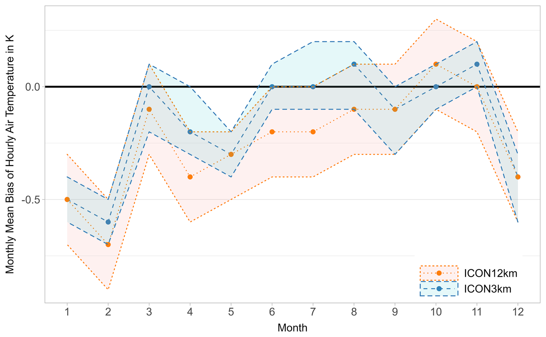
Figure 2 Monthly mean bias of hourly air temperature of ICON3km and ICON12km for the period from 2005 to 2014, as well as the 95 %-confidence intervals from the station means.

3.1.2 Global Radiation

Both ICON3km and ICON12km compute daily mean global radiation significantly higher than observed according to a Welch two sample t-test (${\stackrel{\mathrm{‾}}{G}}_{\mathrm{ICON}\mathrm{3}\mathrm{km}}=\mathrm{45.9}$ J cm⁻², ${\stackrel{\mathrm{‾}}{G}}_{\mathrm{ICON}\mathrm{12}\mathrm{km}}=\mathrm{45.9}$ J cm⁻², ${\stackrel{\mathrm{‾}}{G}}_{\mathrm{Obs}}=\mathrm{44.5}$ J cm⁻²). However, if it is assumed that the observations are systematically too low by 3 %, which is also the pyranometers' measurement uncertainty (DWD, 2023), the apparent overestimation by the climate models is not significant any more. Indeed, pyranometers face the challenge of temperature differences between their inner dome and detector, caused by infrared radiation from the instrument optics in conjunction with different thermal capacities and connectivities (Philipona, 2002), and further intensified by differential cooling by the colder sky, especially on cloud-free days (Sanchez et al., 2015). These effects lead to thermal negative offsets if not controlled sufficiently well, and hence to an underestimation of global radiation by the pyranometers (Philipona, 2002; Sanchez et al., 2015). Daily global radiation estimates by ICON3km were also not found to be significantly different from those computed by ICON12km.

Both climate models were found to overestimate the frequency of daily mean global radiation for the range of bins between 45.7 and 106.7 J cm⁻² but underestimate the frequency of higher global radiation (see Fig. S7). A similar picture can be drawn for the intensity estimates of global radiation. The climate models show a positive bias in the intensity of moderate daily mean global radiation. Extremes however were underestimated.

For most months of the year, the studied CPRCM does not offer noticeable improvement in the estimation of daily mean global radiation, apart during the peak of summer (July), where ICON3km was found to reduce the negative monthly mean bias of daily mean global radiation by 2.5 J cm⁻² (see Fig. S8). For reference, average daily mean global radiation in July was of 77.4 J cm⁻².

When looking at the diurnal cycle of global radiation, estimates from the climate models peak one hour earlier than the observations, however they are able to adequately represent the amplitude of the diurnal cycle (Fig. 3). No apparent improvement is offered by ICON3km compared to ICON12km.

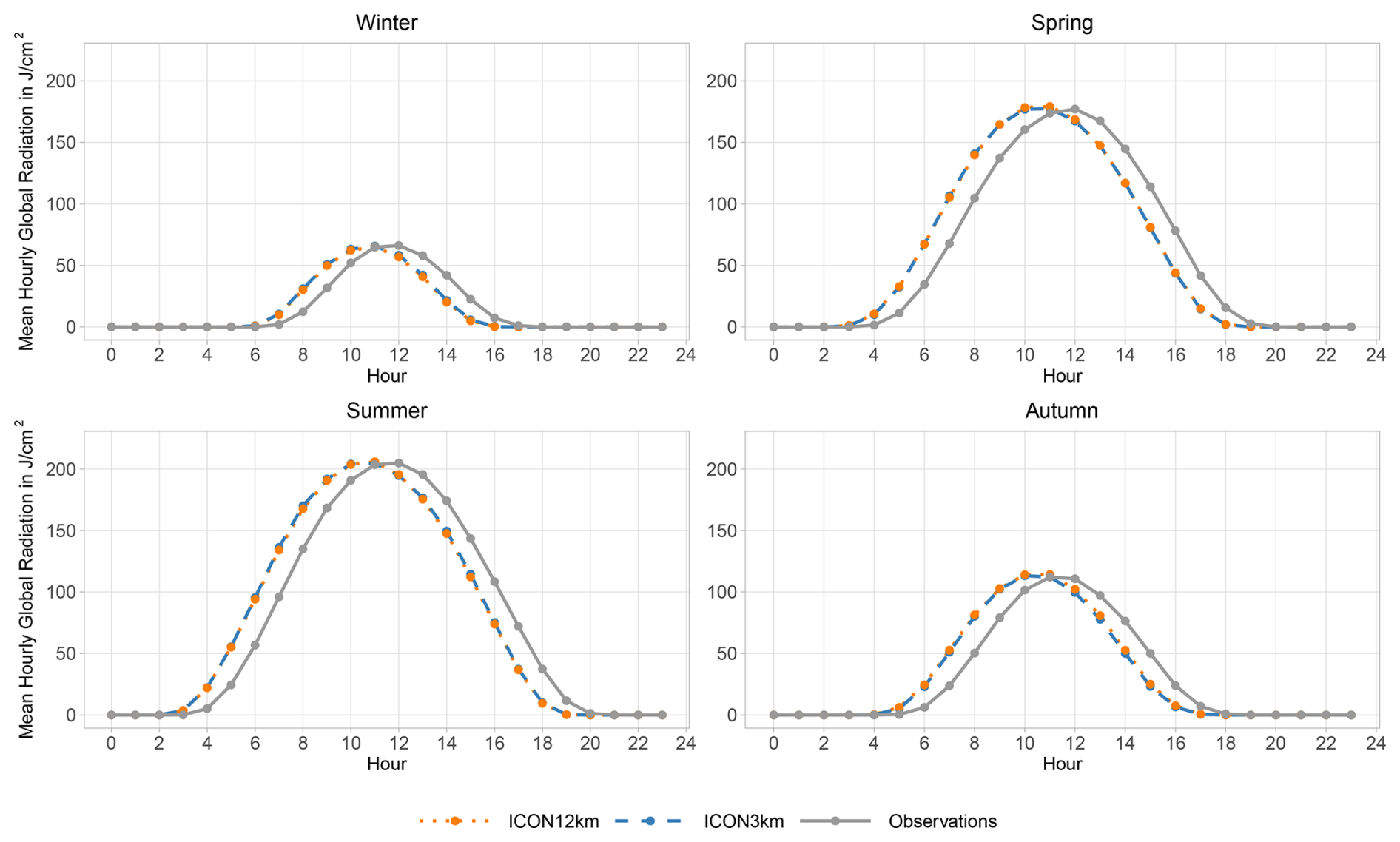
Figure 3 Seasonal diurnal cycles of mean hourly global radiation computed by ICON12km and ICON3km, as well as the observations for the study area for the period from 2005 to 2014.

3.1.3 Relative Humidity

While hourly relative humidity computed by ICON3km is significantly higher than observed (${\stackrel{\mathrm{‾}}{\mathrm{RH}}}_{\mathrm{ICON}\mathrm{3}\mathrm{km}}=\mathrm{78.7}$ % vs. ${\stackrel{\mathrm{‾}}{\mathrm{RH}}}_{\mathrm{Obs}}=\mathrm{78.3}$ %), this is not the case for the estimates by ICON12km according to a Welsh two sample t-test (with ${\stackrel{\mathrm{‾}}{\mathrm{RH}}}_{\mathrm{ICON}\mathrm{12}\mathrm{km}}$ = 78.3 %). Under consideration of the measurement uncertainty of ±2 % of the employed sensor HMP45D (Kyrouac and Theisen, 2017), however neither of the climate models show significant differences to the observations. The estimates by the climate models were found to be statistically significantly different from each other.

ICON12km tends to underestimate the frequency bins of relative humidity of below 46.0 % and of above 89.8 %, while overestimating those between 59.1 % and 89.8 % (see Fig. S9). ICON3km does not seem to offer noticeable improvement in the frequency distribution.

Overall, for most months of the year, monthly mean bias of hourly relative humidity is lower with ICON3km than with ICON12km (see Fig. S10). Only in the months of spring (MAM) was ICON12km found to outperform ICON3km. However, it should be noted that the largest absolute difference in the monthly means of hourly errors between the two models occurs in September and October and is of only 1.3 % relative humidity. These deviations fall within the measurement uncertainty bandwidth. Both climate models tend to show negative relative humidity biases during winter (DJF) and autumn (SON), and positive biases during spring (MAM) and summer (JJA).

3.1.4 Wind Speed

According to a Welch two sample t-test, the climate models show significantly higher mean hourly wind speeds than have been observed (${\stackrel{\mathrm{‾}}{v}}_{\mathrm{ICON}\mathrm{3}\mathrm{km}}=\mathrm{3.4}$ m s⁻¹, ${\stackrel{\mathrm{‾}}{v}}_{\mathrm{ICON}\mathrm{12}\mathrm{km}}=\mathrm{3.2}$ m s⁻¹, ${\stackrel{\mathrm{‾}}{v}}_{\mathrm{Obs}}=\mathrm{3.1}$ m s⁻¹). If the observations are assumed to be systematically too low in the order of the measurement uncertainty, the estimated mean from ICON12km is not significantly different from that of the observations. The measurement uncertainty of the employed anemometers (Ultrasonic Anemometer 2D) is of ±0.1 m s⁻¹ for wind speed below 5 m s⁻¹, and of ±1.5 % for wind speed higher than that (METEK, 2023). Computed wind speeds by ICON3km remain significantly too high in the mean even under consideration of the measurement uncertainty. While this might suggest a performance decline by the CPRCM, it was however found to be the result of an improved representation of the frequency distribution (Fig. 4). Both ICON3km and ICON12km tend to overestimate the frequency of moderate to high wind speeds (2.8 to 11.9 m s⁻¹, resp. 4.0 to 8.5 m s⁻¹), but ICON12km also does so for very low wind speeds (0.6 to 1.7 m s⁻¹), thereby attenuating its positive bias of the mean. While the climate models overestimate the frequency of high wind speeds, they underestimate their intensity, with slight improvements by ICON3km (see Fig. S11).

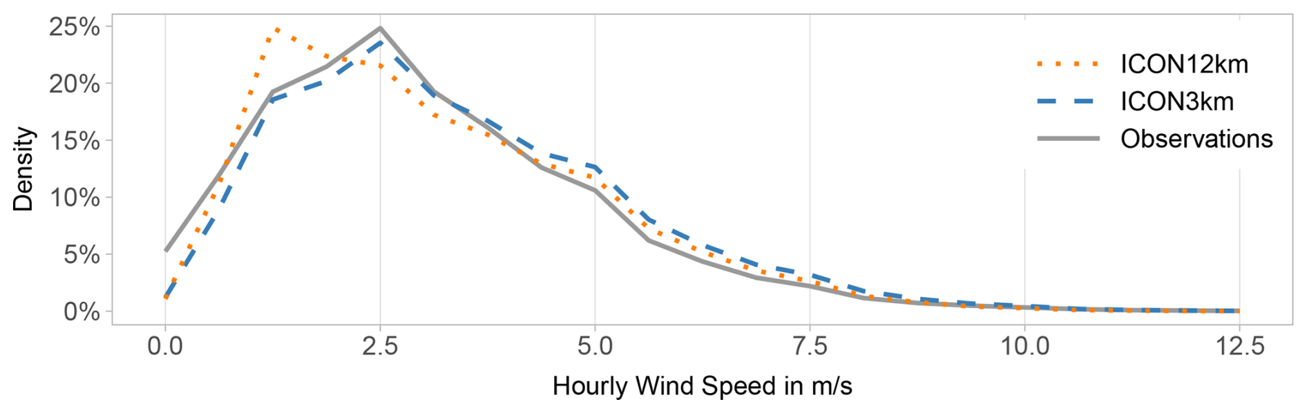
Figure 4 Frequency polygons for hourly wind speed as observed, and calculated by ICON3km and ICON12km over the study area for the period from 2005 to 2014.

ICON12km was found to compute a too pronounced amplitude of the diurnal cycle of hourly wind speed compared to the observations (Fig. 5). ICON3km shows a better performance yet tends to overestimate absolute values. While the observations plateau during the early afternoon, mean wind speed computed by ICON12km drops sharply after having reached its peak around noon, together with solar radiation. Mean wind speed simulations by ICON3km do not show a peak as sharp, but level out shortly, and are thereby in better alignment with the observations.

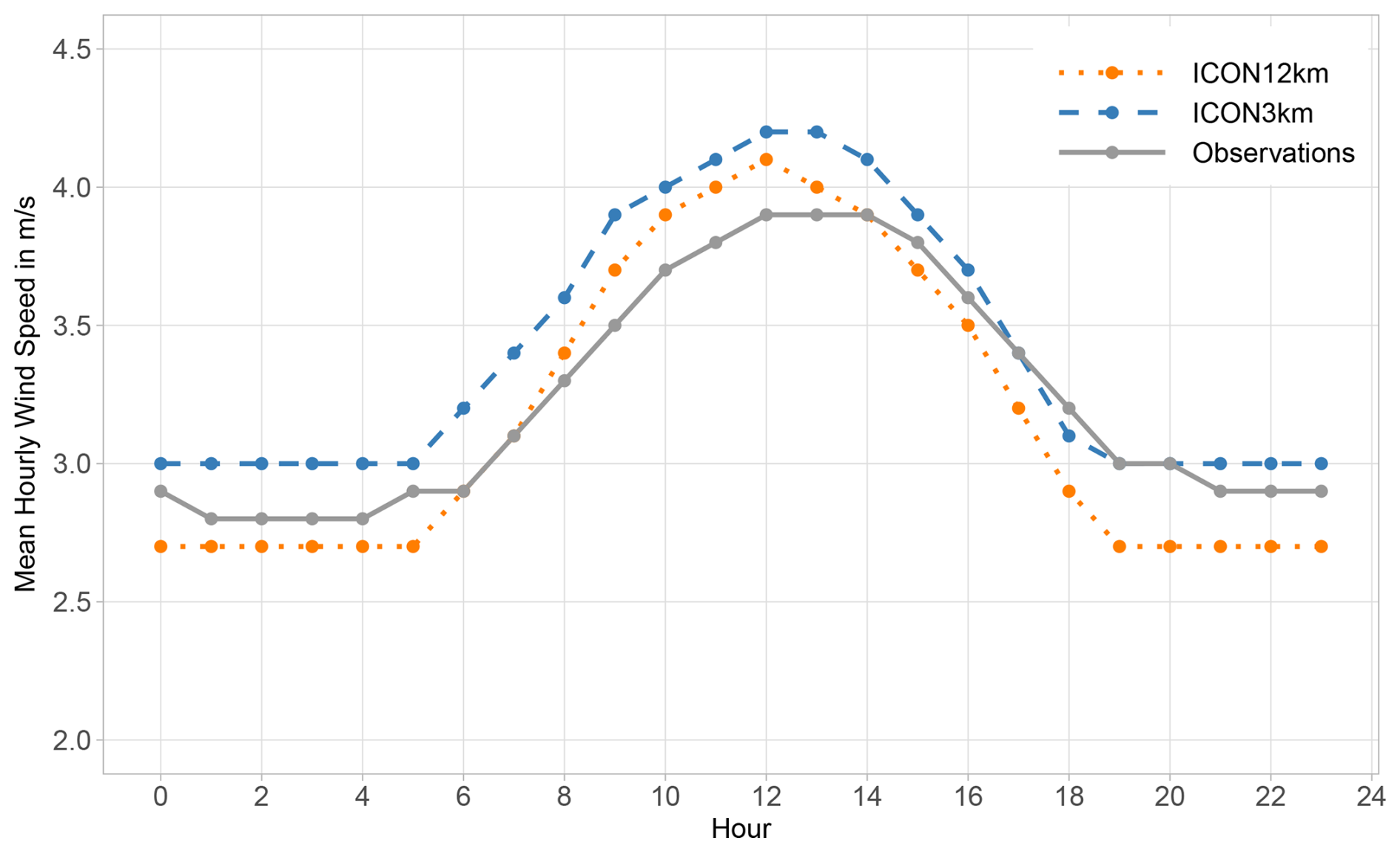
Figure 5 Diurnal cycle of mean hourly wind speed computed by ICON12km and ICON3km, as well as the observations for the study area for the period from 2005 to 2014.

3.1.5 Precipitation

With median hourly precipitation of 4.6 mm over the 99.9th percentile (left-closed interval), ICON12km shows an underestimation compared to adjusted radar data upscaled to the same grid (RADOLAN12km) with a respective estimate of 6.6 mm. In turn, ICON3km overestimates the median of the 99.9th percentile of hourly precipitation compared to upscaled adjusted radar estimates (RADOLAN3km) with 11.6 to 7.3 mm respectively. These trends are further visible in the Q–Q plots (Fig. 6). ICON3km computes unrealistically high hourly rainfall intensities of up to 157.3 mm h⁻¹ over the study region, which is around twice as high as the maximum seen in RADOLAN3km (73.6 mm h⁻¹). Looking exemplarily at all ICON3km hourly precipitation estimates surpassing a chosen threshold of 110 % of the maximum hourly precipitation registered in RADOLAN3km (a total of 146 estimates), these extreme values were found to cover up to 8 cells per time step (see histogram of the number of covered cells per time step in Fig. S12). These extreme estimates all occurred between late April and Mid-September, with a concentration over the summer months. No geographic region in the study area was the main recipient of these storms. An example of such an unrealistic heavy precipitation event can be seen in the simulation time series in July of 2009, when ICON3km computed an area of extreme precipitation with local hourly rainfall intensities of up to 143.3 mm h⁻¹ (peak on 17 July 2009, 17:00 UTC with 6 adjacent cells showing rainfall intensities above 100 mm h⁻¹). In Fig. S13, maps of the precipitation sums for the time window ±12 h around the discussed precipitation peak time in ICON3km are shown for ICON3km, ICON12km, RADOLAN3km and RADOLAN12km. The areal means of the precipitation sums over the study area are of 47.9 mm in ICON3km, 18.6 mm in RADOLAN3km, 18.8 mm in ICON12km and 18.4 mm in RADOLAN12km. This specific event has been chosen for closer hydrological investigation, as the combination of extent and intensity characterises it as one of the most severe downpours simulated. In Sect. 3.2.5, the hydrological impact of this simulated heavy precipitation event is presented.

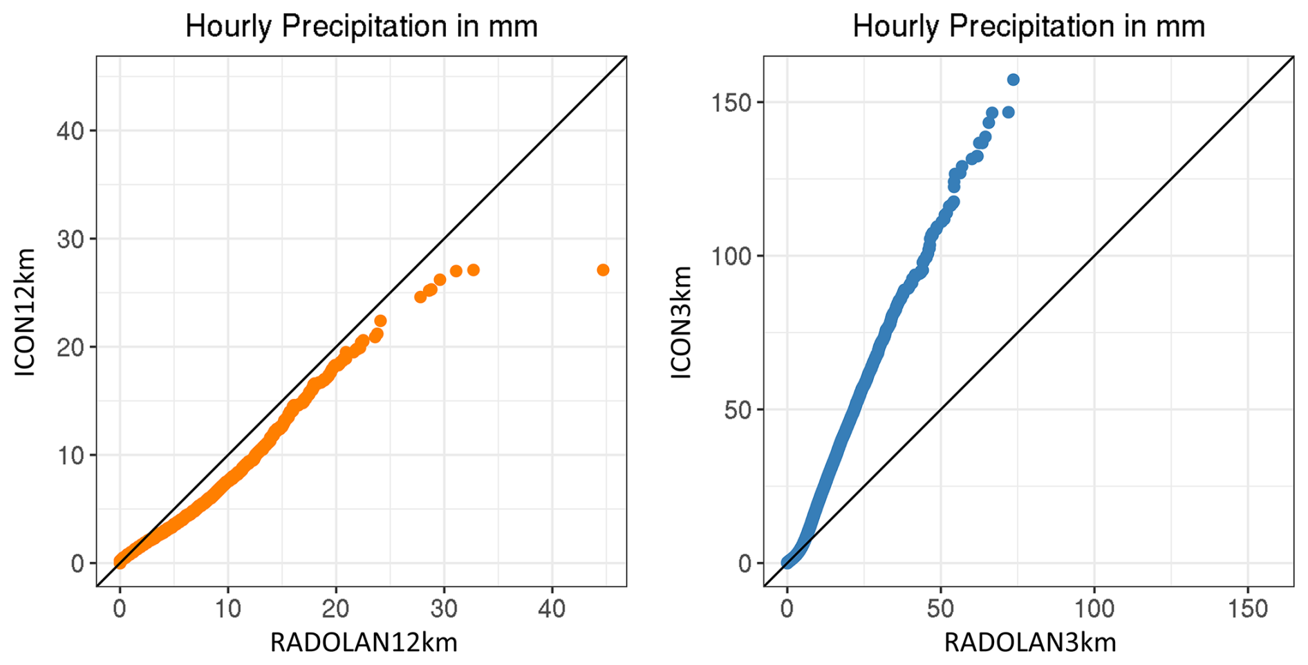
Figure 6 Q–Q plots for hourly precipitation for the period from 2005 to 2014 for ICON12km to RADOLAN12km (left) and ICON3km to RADOLAN3km (right).

The histograms for hourly precipitation are shown in Fig. 7. ICON12km overestimates the frequency of time steps of 0 to 2.9 mm of precipitation (with 7 259 900 counts compared to 7 244 504 counts in RADOLAN12km; bias by ICON12km of 0.21 %; not differentiable in the plot). The overestimation seen in ICON12km has been improved through ICON3km, with ICON3km giving similar counts as RADOLAN3km for precipitation of 0 to 2.9 mm (with 118 011 717 counts and 117 954 139 counts respectively; bias by ICON3km of 0.05 %). The frequency of heavy precipitation on the other hand is consistently underestimated by ICON12km, but overestimated by ICON3km.

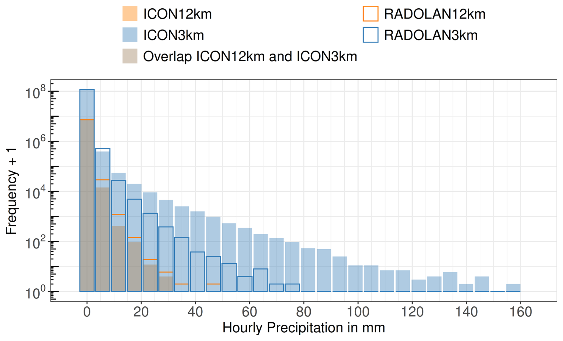
Figure 7 Histograms for ICON12km, ICON3km, RADOLAN12km and RADOLAN3km for hourly precipitation for the period from 2005 to 2014. Note the logarithmic scale of the vertical axis.

The overestimation of high precipitation intensities and their frequencies by ICON3km further results in too high depth-duration-frequency curves, as shown for selected return periods in Fig. 8. In keeping is an overestimation of the mean yearly precipitation totals by ICON3km compared to the radar data upscaled to equal resolution (790 mm compared to 670 mm). An overestimation of the frequency of light precipitation by ICON12km in turn also results in too high mean yearly precipitation totals by ICON12km compared to adjusted radar data estimates of respective resolution (729 mm compared to 665 mm).

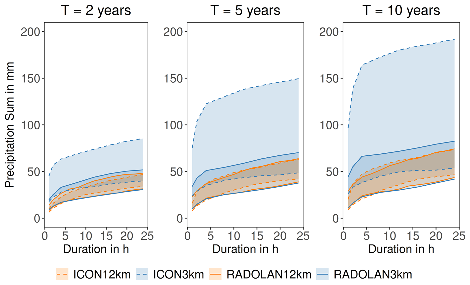
Figure 8 Minimum-maximum bandwidth of the depth-duration-frequency curves from all cells by ICON12km and ICON3km, together with the corresponding estimates from upscaled adjusted radar data (RADOLAN12km and RADOLAN3km) for return periods T of 2, 5 and 10 years.

The monthly means of the deviations of daily catchment-average precipitation computed by ICON3km and ICON12km to the adjusted radar data estimates upscaled to their respective resolution (Fig. S14) are similar between the climate models during autumn (SON) and winter (DJF) but differ more strongly during mid to late spring (April by 0.3 mm, May by 0.4 mm) and during summer (June by 0.3 mm, July by 0.6 mm, August by 0.3 mm). In July, the monthly mean bias of daily catchment-average precipitation is 2.5-times as high for ICON3km than for ICON12km (1.0 to 0.4 mm), given the overestimation of heavy precipitation by ICON3km. Throughout all of April to August, ICON3km gives consistently higher estimates than ICON12km, thereby improving on the negative bias ICON3km shows, with an exception for July, where ICON12km already showed a positive bias, which is only further amplified by ICON3km. It should be kept in mind, that the consideration of daily and catchment-spatial averages entails a smoothing of local extreme hourly precipitation values, dampening their effect.

Precipitation anomalies to the long-term mean are studied to identify how well the climate models are able to depict months with unusual wet conditions (positive precipitation anomalies) and unusual dry conditions (negative precipitation anomalies), as well as potential performance differences between these conditions. Positive monthly precipitation anomalies were found to be predominantly overestimated by the climate models (Fig. 9), especially by ICON3km. This is also reflected in the overestimation of the mean yearly precipitation sums discussed earlier. However, the climate models were still found to be able to reach into the deep negative monthly precipitation anomalies, sometimes even overestimating them. For a considerable number of months, the negative anomalies remain however underestimated, making the picture not as clear cut as for the depiction of positive precipitation anomalies. The same holds true when it comes to the performance comparison of ICON3km and ICON12km.

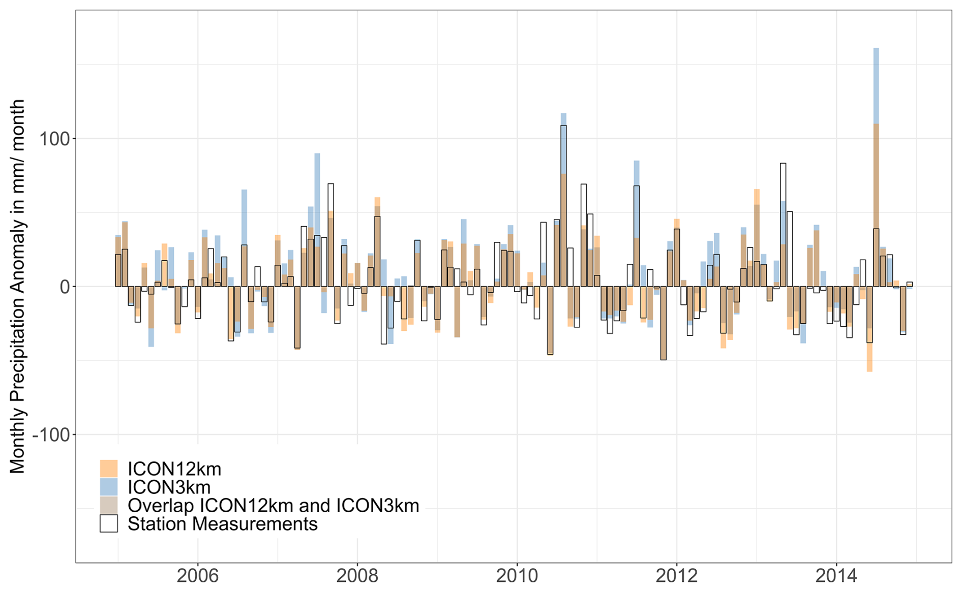
Figure 9 Monthly precipitation anomalies to the long-term reference (1963–2022) for the years 2005 to 2014 for ICON12km, ICON3km and the station measurements.

3.2 Hydrological Analysis

3.2.1 Calibration and Validation of the Hydrological Model

The hydrological model was calibrated manually and validated for its hourly discharge on a distinct flood, and for its weekly discharge on a one-year time series. Thiessen-interpolated meteorological point measurements were used to perform the calibration and validation.

For calibration, the largest summer flood in the area during the study period (flood of June 2013, time window: 31 May 2013, 00:00 to 6 June 2013, 23:00) was considered, looking at the seven catchments for which discharge observations were available. The flood occurred as a result of long-lasting rainfall, brought about by a low-pressure system over East Central Europe, which led to warm moist air being brought from Southern Europe to Germany (LHW, 2014). At Zeitz, peak discharges were measured of an estimated return period of 100 years (LHW, 2014). Nash-Sutcliffe efficiency (NSE) values range between 0.63 and 0.95 and Kling–Gupta efficiency (KGE) values between 0.76 and 0.96 for six of these catchments, while the catchment of Weida constitutes an outlier with a NSE of only 0.14 and a KGE of 0.60. The calibration results are shown in Fig. S15. The simulated responses generally fell short on depicting the flashiness of the catchments and all but two of them (viz. Eisenhammer and Zeitz) showed a retardation of the flood peak. Furthermore, the baseflow was found to be erroneously modelled as barely responsive. The model was validated on the winter flood of 2011 (time window: 7 January 2011, 00:00 to 24 January 2011, 23:00), given that no other pronounced summer flood occurred during the study period. The flood was induced by rapid melting of an unusually thick snow layer in conjunction with heavy rainfall (LHW, 2011). The return period of the measured peak discharge at the gauge Zeitz was of 10 years and at the gauge Kleindalzig of >25 years (LHW, 2011). The model was found to greatly overestimate direct discharge from snowmelt, computing too high and retarded flood peaks, as well as too flashy hydrographs, with a persisting underestimation of the baseflow response.

The model was furthermore calibrated and validated on measured weekly discharge of the years of 2012 and 2008 respectively, as these years are characterised by low monthly precipitation anomalies. The weeks of the year were defined according to ISO 8601. Validation shows that the model overestimates weekly direct discharge, interflow and baseflow.

Assuming the simulated discharges to be systematically distorted by the hydrological model, a qualitative comparison between the concurrent hydrological responses computed based on ICON and RADOLAN data is still possible.

Discharge results from the calibration of the model on the flood of 2013 using Thiessen-interpolated point-based observational data are almost identical to simulations of the same event using RADOLAN precipitation estimates (see Fig. S16). As such, the RADOLAN simulations are considered as reference in the climate model evaluations.

3.2.2 Soil Moisture

Mean hourly relative soil moisture in the hydrological model driven with ICON3km is at 0.144 m³ m⁻³ and thereby significantly higher than in the hydrological model driven with ICON12km, where it is at 0.130 m³ m⁻³. The hourly soil moisture simulations driven with the climate model data are furthermore significantly different in the mean to the results obtained with RADOLAN input data of equal resolution. In fact, the hydrological model driven with ICON3km shows an overestimation of mean hourly soil moisture compared to when driven with RADOLAN3km (${\stackrel{\mathrm{‾}}{\mathrm{SM}}}_{\mathrm{ICON}\mathrm{3}\mathrm{km}}=\mathrm{0.144}$ m³ m⁻³, ${\stackrel{\mathrm{‾}}{\mathrm{SM}}}_{\mathrm{RADOLAN}\mathrm{3}\mathrm{km}}=\mathrm{0.135}$ m³ m⁻³). When driven with ICON12km in turn, mean hourly soil moisture is underestimated by the hydrological model compared to when driven with RADOLAN12km (${\stackrel{\mathrm{‾}}{\mathrm{SM}}}_{\mathrm{ICON}\mathrm{12}\mathrm{km}}=\mathrm{0.130}$ m³ m⁻³, ${\stackrel{\mathrm{‾}}{\mathrm{SM}}}_{\mathrm{RADOLAN}\mathrm{12}\mathrm{km}}=\mathrm{0.133}$ m³ m⁻³). The overestimation, resp. underestimation is not only reflected in the mean over the entire time series, but also shows for the individual months of the year, as seen in the monthly mean biases (with an exception for April, where the bias using the ICON12km driving data is zero, see Fig. S17).

In fact, the soil moisture bias in the hydrological model driven with ICON12km is found to be negative for all quantiles compared to when driven with RADOLAN12km (Fig. 10). Looking at the model driven with ICON3km in relation to when driven with RADOLAN3km, the sign of the soil moisture bias however becomes positive for moderate to high soil moisture.

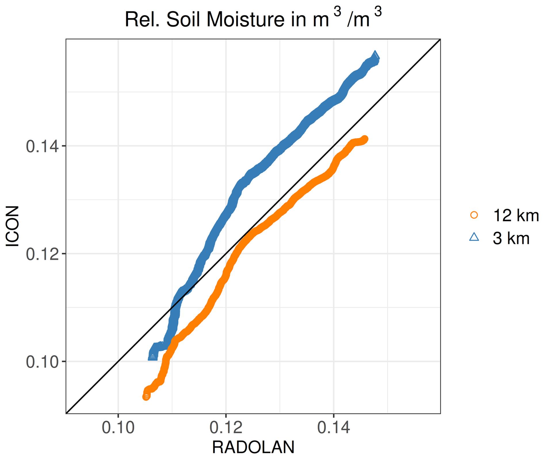
Figure 10 Q–Q plots for hourly soil moisture for the period from 2006 to 2014 for ICON12km to RADOLAN12km and ICON3km to RADOLAN3km.

3.2.3 Total Evapotranspiration

Mean hourly total evapotranspiration is higher in the hydrological model driven with ICON3km than when driven with ICON12km (${\stackrel{\mathrm{‾}}{\mathrm{ET}}}_{\mathrm{ICON}\mathrm{3}\mathrm{km}}=\mathrm{32.96}\times {\mathrm{10}}^{-\mathrm{3}}$ mm, ${\stackrel{\mathrm{‾}}{\mathrm{ET}}}_{\mathrm{ICON}\mathrm{12}\mathrm{km}}=\mathrm{32.56}\times {\mathrm{10}}^{-\mathrm{3}}$ mm). However, both ICON models lead to mean hourly total evapotranspiration values lower than the RADOLAN products of equal resolution (${\stackrel{\mathrm{‾}}{\mathrm{ET}}}_{\mathrm{RADOLAN}\mathrm{3}\mathrm{km}}=\mathrm{32.99}\times {\mathrm{10}}^{-\mathrm{3}}$ mm, ${\stackrel{\mathrm{‾}}{\mathrm{ET}}}_{\mathrm{RADOLAN}\mathrm{12}\mathrm{km}}=\mathrm{33.02}\times {\mathrm{10}}^{-\mathrm{3}}$ mm). It is however to be noted that none of these differences are significant according to a Welch two sample t-test at 95 % confidence level.

The annual cycle of the monthly mean bias of hourly catchment-average total evapotranspiration is shown in Fig. 11. The bias of ICON3km to RADOLAN3km deviates most strongly from the bias of ICON12km to RADOLAN12km in the summer months (JJA). For this time period, the negative bias of the driving model ICON12km is shifted to a positive bias by the nested model ICON3km.

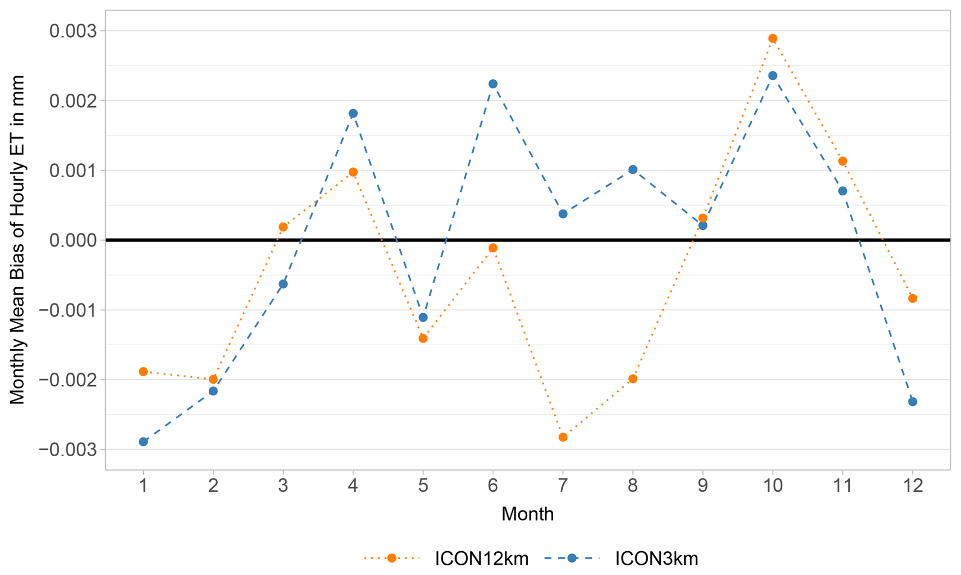
Figure 11 Monthly mean bias of hourly total evapotranspiration, as calculated by the hydrological model driven with ICON3km and ICON12km for the period from 2006 to 2014.

3.2.4 Continuous Discharge Simulation

The hydrological model driven with meteorological data from ICON12km was found to compute median hourly discharge values for the study period from 2006 to 2014 that are lower than when driven with adjusted radar data of the same resolution (RADOLAN12km) (Fig. 12). In turn, when driven with data from ICON3km, the hydrological model simulated median hourly discharges that were higher than estimates based on adjusted radar data of equal resolution (RADOLAN3km).

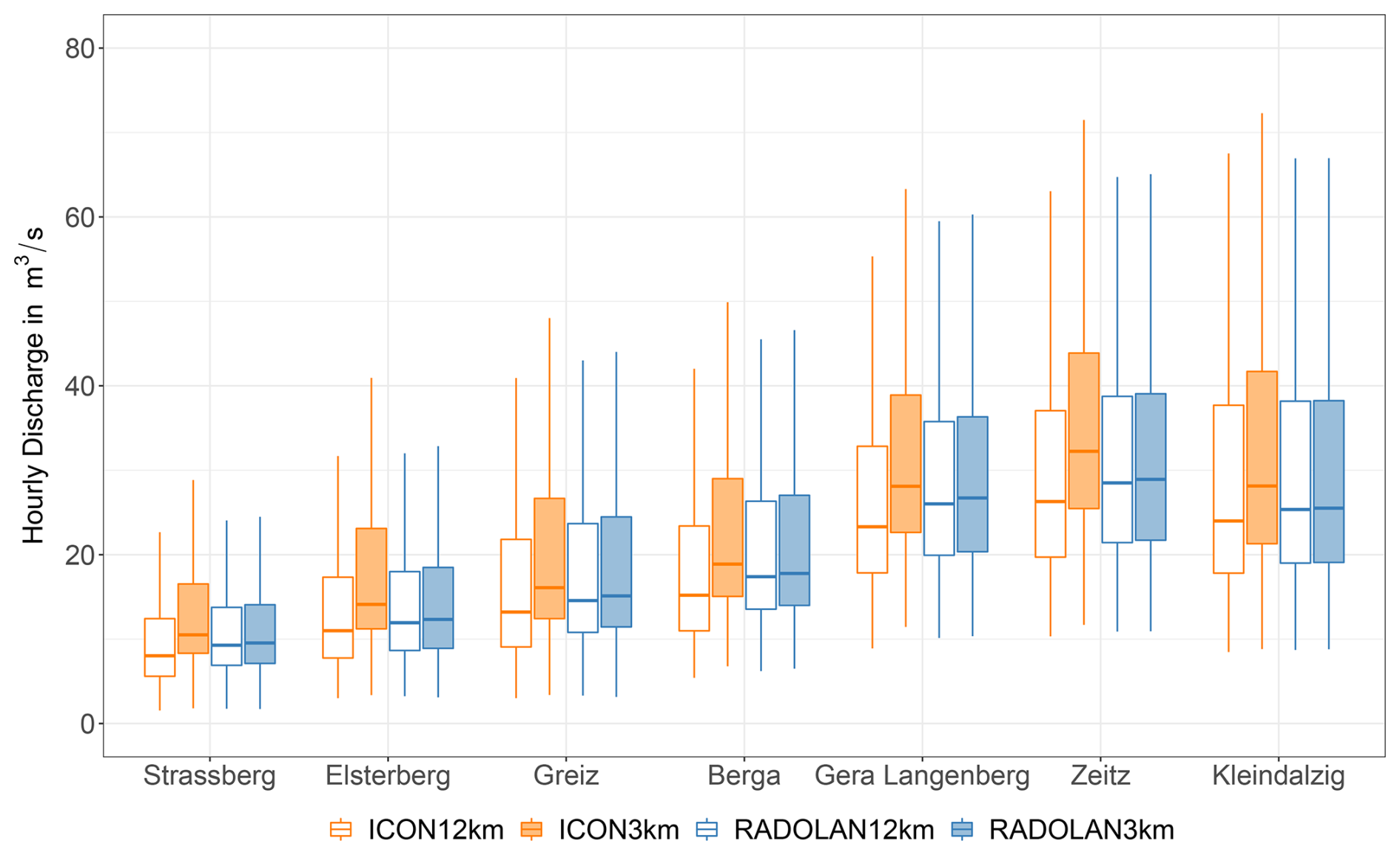
Figure 12 Boxplots of hourly discharge (period from 2006 to 2014) computed by the WaSiM hydrological model driven with meteorological data from ICON12km and ICON3km, as well as with adjusted radar data of respective equal resolution (RADOLAN12km and RADOLAN3km) for catchments of the main stem of the Weiße Elster river within the study area. Values beyond the whiskers are not represented.

The frequency distributions show too frequent low flows for the hydrological model driven with ICON12km and too frequent high flows when driven with ICON3km for nine out of the twelve studied catchments (with the exception of Eisenhammer, Dröda and Mylau, all of which are independent feeding catchments).

The temporal variability of the monthly mean bias of hourly discharge is similar for all studied catchments and was found to be strongly shaped by the annual cycle of precipitation bias. During winter (DJF) and early spring (March and April), the hourly discharge estimates based on the climate model data deviate to a similarly strong degree from simulation results obtained based on adjusted radar data of respective resolution (Fig. 13). However, for summer (JJA) the climate models' biases are markedly different to each other due to the pronounced overestimation of convective precipitation by ICON3km.

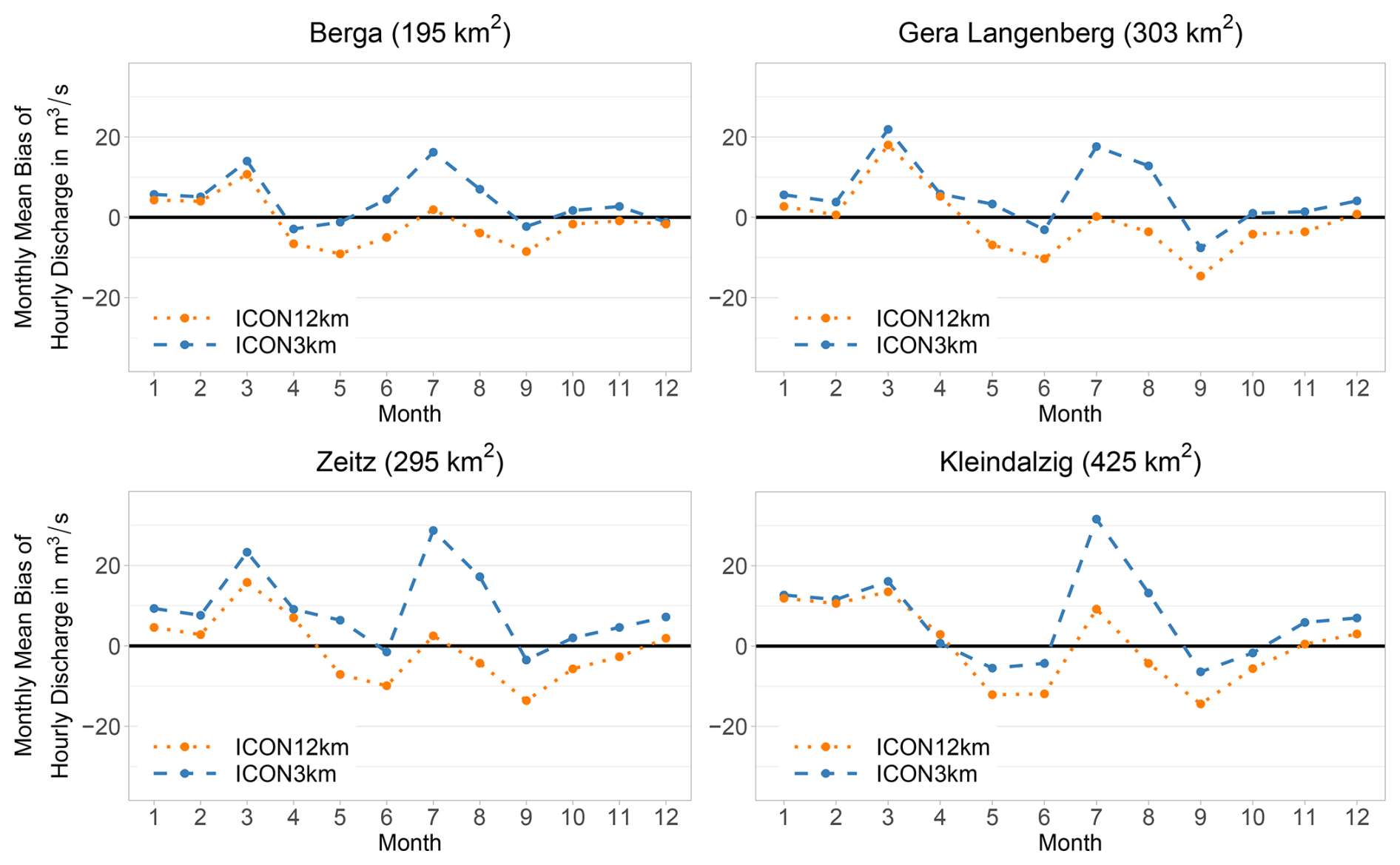
Figure 13 Monthly mean bias of hourly discharge from the hydrological model driven with ICON12km/ICON3km meteorological data compared to when driven with adjusted radar data of equal resolution (RADOLAN12km/RADOLAN3km) for the four most downstream catchments on the main stem of the Weiße Elster river within the study area for the period from 2006 to 2014.

Driving the hydrological model with ICON12km meteorological data was found to lead to an underestimation of median hourly discharge, but results in an overestimation when looking only at the 99.5th percentile of hourly discharge for six out of the seven catchments on the main stem (see Fig. S18). The use of ICON3km data as input to the hydrological model in turn leads to an overestimation of median hourly discharge among both the complete dataset and the 99.5th percentile. The interquartile range of the 99.5th percentile of hourly discharge computed by the hydrological model driven with climate model data (ICON12km/ICON3km) is found to be larger than when driven with meteorological observations (RADOLAN12km/RADOLAN3km).

Figure 14 shows the relation between runoff and the sum of total rainfall volume and 8 d antecedent rainfall for simulations with ICON12km, ICON3km, RADOLAN12km and RADOLAN3km. The segmented regression is highly sensitive to rainfall-runoff events of high return period, such as predominantly recorded from the ICON model simulations. As such, no firm conclusions can be drawn from Fig. 14 on the existence or position of a break point in the relation between runoff and rainfall.

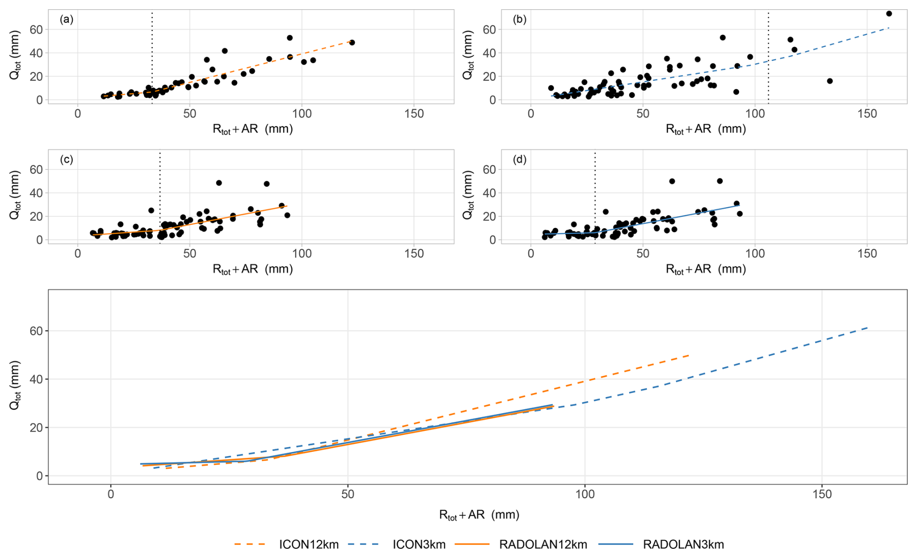
Figure 14 Upper half: Scatter plots of total runoff (Q_tot) to the sum of total rainfall (R_tot) and 8 d antecedent rainfall (AR) over the catchment of Kleindalzig and those upstream, fitted with a piecewise linear regression model for (a) ICON12km, (b) ICON3km, (c) RADOLAN12km and (d) RADOLAN3km. The thresholds are indicated with a dotted vertical line. Lower half: Combined piecewise linear regression model results of Q_tot to R_tot + AR.

3.2.5 Event-based Simulation

The model results for the largest flood that occurred during the study period, namely the flood of June 2013 (which is also the calibration event), are shown in Fig. 15 exemplarily for the catchment furthest downstream in the study area for which discharge measurements are available. Both climate models described a heavy precipitation event occurring too shortly with a peak earlier than observed. As a result, the hydrographs simulated based on ICON3km and ICON12km are too narrow and peak too early. Driven with RADOLAN3km and RADOLAN12km, the soil moisture results suggest that the storm rained off over saturated soils; the precipitation event did not lead to an increase of soil moisture, but to a pronounced runoff peak. In turn, ICON12km as climate input data leads to too low soil moisture, allowing for a buffering of the flood wave by the soils and an attenuation of the flood peak. ICON12km was found to underestimate the peak daily rainfall intensity of the storm. ICON3km in turn strongly overestimated it. While antecedent soil moisture in the hydrological model driven with ICON3km was similar to when driven with RADOLAN3km, however the rainfall by ICON3km likely fell over catchments with not yet fully exhausted storage capacities. In fact, the average soil moisture in the hydrological model driven with ICON3km rose, leading to a reduction of the flood peak, thereby buffering the large overestimation of daily rainfall intensity seen in ICON3km.

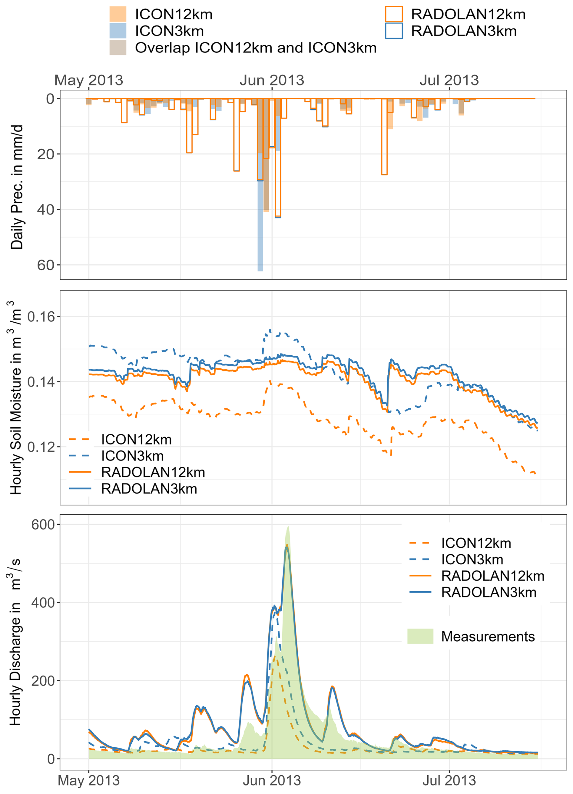
Figure 15 Top: Daily spatial average precipitation estimates over the catchment of Zeitz and those upstream for the period of the 2013 flood for ICON12km, ICON3km, RADOLAN12km and RADOLAN3km, Centre: the respective hourly relative soil moisture spatial averages gained from continuous simulation, Bottom: the resulting hydrographs (using hourly data) for the catchment of Zeitz together with the discharge measurements.

Throughout the data series, ICON3km shows a number of unrealistically high precipitation intensities, occurring predominantly in summer, and of which many are clustered. This has been discussed in Sect. 3.1.5, and an example of one of the most severe downpours simulated by ICON3km was presented. In the following, it is shown how this selected heavy precipitation event translates into discharge in the Weiße Elster river basin. Despite showing a maximum hourly precipitation intensity of 143.3 mm h⁻¹ (17 July 2009, 17:00), the resulting peak discharge at Zeitz was of only 198 m³ s⁻¹, which is somewhat lower than measured during the winter flood of 2011 (peak discharge: 253 m³ s⁻¹), to which a return period of 10 years was attributed (LHW, 2011). The extreme overestimations of precipitation intensity in ICON3km occur primarily in summer and are strongly confined in space and time. The available soil storage capacity in summer is usually high, the antecedent discharge in the river low, and precipitation volumes are restricted given the limited spatial and temporal extent of the simulated storms. As a result, the discharges simulated from such unrealistically heavy downpours are within the range of recent observations at the catchment outlet.

4 Discussion

Here we identify strengths and limitations of the studied CPRCM in depicting hourly air temperature, global radiation, relative humidity, wind speed and precipitation over a chosen medium-size river basin in Germany, and compare these to conclusions from other studies. Previous research efforts have mainly focused on precipitation, with only few discussing other meteorological variables (Lucas-Picher et al., 2021) and seldomly for medium to small basins, but rather on larger subnational scale. Furthermore, it is discussed how the performance results from the use of the analysed CPRCM data for hydrological impact modelling compare to previous studies on other river basins with varying model chains.

4.1 Near-Surface Air Temperature

While both the studied RCM (ICON12km) and the CPRCM (ICON3km) were found to compute mean hourly air temperatures lower than observed, the deviations fall within the measurement uncertainty bandwidth. Hackenbruch et al. (2016) also showed a cold bias for COSMO-CLM at 2.8 and 7.0 km resolution over southwestern Germany, and so did Tölle et al. (2018) for COSMO-CLM at 1.3 and 7.0 km resolution over central Germany. These studies found higher bias in summer than in winter, however our results show the opposite, likely due to the predominance of cropland and pasture in our study area (cf. Fig. S1). Over open land, cold biases are amplified due to higher albedo and shorter roughness lengths, the latter favouring the development of stable atmospheric conditions and allowing for stronger nocturnal cooling (Lind et al., 2020). These results underline the importance of scale and exemplarily show how dominating processes on the catchment scale can differ from those over larger study areas.

The CPRCM (ICON3km) was found to offer improvement for air temperature simulations in the summer months, in keeping with a variety of other studies conducted over Europe (Prein et al., 2015). These improvements have been linked to deep convection being explicitly resolved, which allows for better estimates of deep-convective clouds (Leutwyler et al., 2017; Hentgen et al., 2019) and a better representation of convective precipitation (Liu et al., 2017).

Furthermore, ICON3km exhibited a slightly lower spatial bias variability throughout the year compared to ICON12km, as reflected by the 95 % confidence interval from the station means. This finding is in line with Xie et al. (2025) who saw higher spatial variability in temperature bias by the RCM they used over western Norway compared the use of a CPRCM.

4.2 Global Radiation

Both ICON3km and ICON12km were found to overestimate mean daily global radiation over the study area, however the deviations were not significant under consideration of the measurement uncertainty. Hackenbruch et al. (2016) found an underestimation of half-year mean sums of global radiation over southwestern Germany (1983–2000) for COSMO-CLM at 2.8 and 7.0 km resolution. In our study an underestimation was registered for the highest quantiles of daily global radiation both in intensity and frequency. ICON3km was able to reduce this bias. Through a better estimation of the onset of convection in the summer mornings and resulting reduced stratification, CPRCMs were shown to be able to dampen the RCMs' positive bias in the estimation of the frequency of high clouds (Keller et al., 2016). The simulation of more frequent clear-sky conditions allows for a reduction in the underestimation of global radiation (Keller et al., 2016; Leutwyler et al., 2017; Hentgen et al., 2019).

4.3 Relative Humidity

The skill of CPRCMs in depicting relative humidity is seldomly studied, however it has been shown that an increase in relative humidity constitutes a critical factor in deep convective initiation (Morrison et al., 2022).

No significant differences in mean hourly relative humidity were found for ICON3km or ICON12km compared to the observations under consideration of the measurement uncertainty. Monthly bias means proved negative for winter and autumn, but positive for spring and summer for both the RCM and CPRCM. Hackenbruch et al. (2016) found median relative humidity biases computed by COSMO-CLM at 2.8 and 7.0 km resolution over southwestern Germany to be positive for both half years, with biases much greater than seen for the ICON-CLM models. Possible explanations for the smaller biases in our study might be improvements to the model physics in the newer ICON-CLM (version 2.6.4) compared to the COSMO-CLM model they used, or differing model parametrisations.

4.4 Wind Speed

ICON3km was found to estimate higher wind speed extremes than ICON12km, thereby slightly improving on the underestimation of extremes shown by both climate models. This result is in line with Iles et al. (2020), who found an increase in intensity and frequency of high winds with resolution, when comparing climate models of 12.5 and 50 km resolution over the European domain. Similar trends were found by Kunz et al. (2010) when comparing REMO-UBA at 10 km resolution and COSMO-CLM at 18 km resolution over Germany. ICON3km improved on the depiction of the frequency of light winds (0.6 to 1.7 m s⁻¹) computed by its driving model ICON12km, however both show an overestimation of the frequency of high wind speeds. As such, the simulation of wind speed remains a challenge for both climate models. Belušić et al. (2018) advance that it takes grid spacings of a few kilometres to accurately simulate small-scale wind systems. Hackenbruch et al. (2016) prove added value for the use of a CPRCM of 2.8 km resolution for the computation of channelled wind flow in the Neckar Valley and underline the importance of orographic structures for the initialisation of local wind systems.

4.5 Precipitation

ICON12km was found to compute too frequent light precipitation, while underestimating the intensity of heavy rainfall. ICON3km improves on the frequency estimation of light precipitation but overestimates the intensity of the highest quantiles. A reduction in the frequency of light precipitation and an increase in the intensity of heavy precipitation by the CPRCM compared to its driving RCM is in line with the consensus from literature (Lucas-Picher et al., 2021), e.g. with Ban et al. (2021) and Adinolfi et al. (2021). Ban et al. (2021) studied a 23-member ensemble of CPRCMs run at 3 km resolution and their driving RCMs at 12 km and found the CPRCMs to be able to alleviate the RCM-ensemble negative mean bias seen in the 99.9th-precipitation-percentile. In fact, the CPRCM-ensemble shows a respective mean bias within the acceptable range considering measurement uncertainty for all study areas and seasons, except winter (DJF) in Switzerland and summer in Italy (JJA) where the negative bias is weakened but remaining (Ban et al., 2021). Ban et al. (2021) furthermore found improvement through reduced wet-hour frequency by the studied CPRCM-ensemble. Adinolfi et al. (2021) show similar improvement by the CPRCM they analysed over an Alpine domain, stretching from central Italy to northern Germany, reducing precipitation frequency and increasing precipitation intensity compared to the driving RCM. Nevertheless, within the 99.9th percentile, the CPRCM intensity estimates remain slightly too low for precipitation values lower than 6 mm h⁻¹, but the CPRCM overestimates heavy precipitation higher than 6 mm h⁻¹ (Adinolfi et al., 2021). In their study over the southern United Kingdom, Kendon et al. (2012) showed an RCM of 12 km resolution to compute heavy rainfall as not intense enough, but as too persistent and widespread. A CPRCM of 1.5 km resolution in turn achieved improvements in the frequency distribution, duration and spatial extent, but estimated too intense heavy rainfall (Kendon et al., 2012). Xie et al. (2025) found an overestimation of annual maximum 1 d precipitation and maximum 1 h precipitation using the HARMONIE climate model in convection-permitting set-up at 3 km resolution compared to running it at coarser resolution (12 km) with parametrised convection. However, they found the CPRCM to outperform the RCM in capturing hourly precipitation above the 95th percentile (Xie et al., 2025).

RCMs with convective parametrisation have shown to underestimate heavy rainfall. In fact, small atmospheric instabilities are sufficient to trigger the convection schemes in the RCMs, leading to the release of light rain and thereby inhibiting a greater computational built-up of the convective cells (Ban et al., 2021). Parametrisation schemes were designed de facto to represent average effects at coarse resolution, however not localised extreme events and individual storms (Kendon et al., 2012).

CPRCMs in turn tend to overestimate the intensity of heavy rainfall, as updrafts are computed as too wide under the coarseness of the model grid (Kendon et al., 2023). Additionally, entrainment is insufficiently captured due to turbulence not being sufficiently resolved in the convective cells (Bryan and Morrison, 2012 cited in Quintero et al., 2022).

ICON3km was found to compute unrealistically high hourly rainfall intensities of up to 157.3 mm h⁻¹ over the study region, which is around twice as high as the maximum seen in RADOLAN3km (73.6 mm h⁻¹). These extremely high rainfall intensities were primarily estimated in the summer, and most were seen to cluster spatially and extend over several consecutive time steps. They are consequently likely the result of shortcomings in the parametrisation of the microphysics, rather than randomness or numerical instability.

ICON12km was found to compute too high mean annual precipitation totals, likely because of an overestimation of wet-hour frequency. This result is in agreement with findings by Strandberg and Lind (2021) for a 12.5 km resolution RCM over the European domain. The underestimation of average daily precipitation sums by RADOLAN compared to ground-truth rain gauge data (Kreklow et al., 2020) further exacerbates this positive bias.

The deviations of ICON3km and ICON12km to the adjusted radar data estimates upscaled to their respective resolution were found to be similar between the climate models during autumn and winter but differing most strongly during the peak of summer. In fact, synoptic weather systems, which are dominant in winter, are well represented even in coarse climate models (Strandberg and Lind, 2021) and the CPRCM is likely not providing much additional information or added value to their depiction. For summer however, when small-scale convective processes are at the forefront, the explicit representation of convection in the CPRCM likely leads to pronounced differences compared to estimates by its driving RCM where convection is parametrised (Strandberg and Lind, 2021).

Monthly negative precipitation anomalies were not found to be better represented by ICON3km than by ICON12km. They are predominantly shaped by large-scale atmospheric circulations, handed over to the CPRCM as lateral boundary conditions by its driving RCM. Taylor et al. (2013) however found a change from positive to negative in the sign of the soil-moisture precipitation feedback over their semi-arid domain when switching from an RCM with parametrised convection to a CPRCM. A negative feedback makes a drought less likely, whereas a positive feedback may prolong or intensify it (Taylor et al., 2013). Kendon et al. (2019) further show over an Africa-wide domain, that the use of a CPRCM (4.5 km resolution) can be of added value for the estimation of the length of dry spells through a more accurate depiction of the triggering of diurnal rainfall and an improved representation of the dying out of westward propagating systems.

4.6 Soil Moisture

Reszler et al. (2018) looked at soil moisture on a monthly basis and found estimates from a hydrological model driven with CPRCM data to be similar in winter and spring to those when using RCM input data, however the estimates deviate considerably in summer and autumn. In fact, during summer and autumn both climate models underestimate soil moisture, but the CPRCM is able to reduce the negative bias seen in the hydrological model driven with RCM data (Reszler et al., 2018). In contrast, ICON3km as input to the hydrological model WaSiM leads to an overestimation of hourly soil moisture throughout the year, while ICON12km leads to an underestimation. However, the results agree with the study of Reszler et al. (2018) on higher soil moisture in summer and autumn by the hydrological model driven with CPRCM data than when driven with RCM data.

4.7 Total Evapotranspiration

Biases in observed and modelled meteorological variables can greatly influence evapotranspiration estimates. Meyer et al. (1989) introduced random and systematic errors to the input data of the Penman method to study the effect of such errors on the estimation of daily potential evapotranspiration. They found that random errors distort potential evapotranspiration estimates in a similar manner than systematic errors. Standard errors in potential evapotranspiration were fairly low when introducing random errors on wind run data, but three times as high when applying random errors of the same scale on temperature data, and four to five times as high when adding the random errors on relative humidity or solar radiation data (Meyer et al., 1989). In climate modelling, however the uncertainty is not equally distributed among variables. Lai et al. (2022) investigated the missing-variable estimation approaches by FAO and how the selection or exclusion of certain climate variables from global climate models shape the uncertainty of projected reference crop evapotranspiration using the Penman-Monteith method. They concluded that air temperature and shortwave radiation should be prioritised given the low projection uncertainty of these variables and high influence on reference evapotranspiration. Kay and Davies (2008) found the uncertainty introduced by the climate model structure to be higher than that by the potential evaporation formulation.

Mendoza et al. (2016) found higher basin-averaged mean annual evapotranspiration estimates in hydrological modelling when using meteorological forcing data from the WRF model at 4 km resolution in convection-permitting set-up than at coarser resolution of 12 or 36 km with parametrised convection. These results are in keeping with the study presented here, where higher mean hourly total evapotranspiration is registered for the hydrological model driven with ICON3km compared to when driven with ICON12km. During summer (JJA), the monthly mean biases of hourly catchment-average total evapotranspiration computed by the hydrological model driven with ICON3km and ICON12km deviate most strongly, with a shift from a negative bias by the driving model ICON12km to a positive bias by the driving model ICON3km. Higher total evapotranspiration by ICON3km, especially in summer, is likely the result of higher water availability through higher precipitation intensities in ICON3km, as well as a reduction of the negative summer bias in temperature and global radiation by ICON3km. Mendoza et al. (2016) also saw a wet bias in the CPRCM they studied. They furthermore analysed the partitioning of basin-averaged mean annual precipitation into basin-averaged mean annual evapotranspiration and found partitioning to be lower when the hydrological model is driven with CPRCM data than when driven with data from the RCMs.

4.8 Discharge Simulations

All the discussed meteorological variables are used as input to the hydrological model and shape through their biases the accuracy of the discharge simulations. The hydrological model WaSiM driven with ICON3km simulates higher discharge than when driven with ICON12km. These findings are in agreement with the consensus from literature. Kay et al. (2015) report higher low flow volumes, median flows and high flow volumes when using CPRCM data compared to when using data from an RCM with parametrised convection. Mendoza et al. (2016) also saw higher basin-averaged mean annual runoff when driving their hydrological model with a CPRCM than with an RCM. Reszler et al. (2018) simulated higher maximum annual flood peaks using data from a CPRCM of 3 km resolution than from an RCM of 12.5 km resolution. Higher peak streamflows were also found by Schaller et al. (2020) using CPRCM data to simulate a selected autumn flood event on the West Coast of Norway compared to the use of GCM data. Davis et al. (2022) simulated higher (maximum) water levels in an urban catchment in India driving their hydrological model with data from a CPRCM ensemble than with data from the Global Forecasting System. Ascott et al. (2023) in turn computed greater daily river flows in the Lake Victoria basin when using CPRCM data compared to the use of RCM data. In keeping, Poncet et al. (2024) and Xie et al. (2025) found higher peak-over-threshold historical flood peak discharges using CPRCM data than when using RCM data to drive their hydrological models. Archer et al. (2024) found larger relative flooded areas from the historical intensity-duration-frequencies derived from a CPRCM ensemble than from interpolated rainfall observations.

Given its strong overestimation of precipitation intensity, ICON3km did not allow for improved discharge simulation compared to ICON12km. Kay et al. (2015) and Reszler et al. (2018) also attributed no added value to the use of their studied CPRCM for hydrological impact modelling. In fact, Kay et al. (2015) found worse performance in discharge computation using the 1.5 km CPRCM compared to using its driving 12 km RCM as input to the gridded hydrological model CLASSIC-GB, given the strong positive precipitation bias of the CPRCM when left uncorrected. Reszler et al. (2018) found deficiencies in the depiction of the temporal distribution of rainfall intensities to be another potential source of error. In a later study, Kay (2022) did however find added value in the use of a 2.2 km CPRCM compared to a 12 km RCM (each 12 member ensembles) for the simulation of daily low flow volume, median flow, and high flow volume across Britain. They attribute these improvements to changes in the physics of the used CPRCM compared to the earlier model employed in their 2015 study (cf. Kay et al., 2015). Also Mendoza et al. (2016), Schaller et al. (2020), Davis et al. (2022) and Poncet et al. (2024) found various added value in the use of CPRCMs for hydrological modelling (cf. Table 1). Xie et al. (2025) only found added value for the simulation of extreme flood peaks, characterised by return periods above 10 years.

The 99.5th percentile of hourly discharge was overestimated in the median by the hydrological model driven with ICON3km, as a result of the overestimation of the intensity of heavy precipitation. The input of ICON12km data to the hydrological model also resulted in an overestimation of hourly discharge of the 99.5th percentile in the median for six out of the seven catchments on the main stem, despite an underestimation of precipitation intensity. In fact, the rainfall-runoff-analysis (Fig. 14) showed a greater number of rainfall-runoff events of high return period when using the climate model data for hydrological modelling than when using meteorological observations. This is reflected through a more strongly scattered rainfall-runoff-plot in comparison to the use of observational meteorological data and translates to a higher interquartile range and a higher median of the 99.5th percentile of hourly discharge for the hydrological model driven with climate model data (Fig. S18). An overestimation of high discharges by the hydrological model driven with RCM data is also apparent in the study of Reszler et al. (2018). For four out of the six catchments they studied, the return periods from the hydrological model driven with 12.5 km RCM data overtake or at least come to match the return period curves from the observations for high return periods, while undercutting them for lower return periods.

We showed exemplarily for the flood event of 2013 in the Weiße Elster catchment that a simulated overestimation in precipitation does not always translate into an overestimation in flood peak discharge, as the storm cell might be shifted in space in the climate model simulation and rain off over soils with greater available storage capacity. In fact, in simulations run over vast domains, such as the Central European (CEU) domain in this study, the general events and patterns can be expected to match, but the climate models are unlikely to perfectly capture the actual geographic position of a local storm.

To conclude, no added value could be found in the use of uncorrected climate model data from ICON3km for hydrological impact modelling, given the overestimation of the intensity and frequency of heavy rainfall by ICON3km. The results presented here are drawn from a short time series (10 years) obtained from a single CPRCM run and reflect the hydroclimatic simulations over a single cluster of catchments. Longer time series, climate model ensembles and additional study areas are needed to draw firm conclusions on the general performance of CPRCMs for hydrological impact modelling.

5 Conclusion

Climate change projections are key for the development of mitigation and adaptation strategies (IPCC, 2023). Policy decisions rely on climate model results that are not only to be of low bias and uncertainty, but also of high spatial and temporal resolution. CPRCMs bear major potential for advancement towards these requirements, as they run on fine model grids and no longer rely on deep-convection parametrisation schemes, which come with great uncertainty (Ban et al., 2021). Yet to this day, their performance in depicting meteorological variables on the catchment scale and their potential added value for hydrological impact modelling is scarcely studied (Lucas-Picher et al., 2021).

In the work presented here, the skill of estimating meteorological variables on the catchment scale is analysed for ICON-CLM 2.6.4 in its convection-permitting setup at 3 km resolution (ICON3km), and for its driving model ICON-CLM 2.6.4 at 12 km resolution with parametrised convection (ICON12km, forced with ECMWF-ERA5). Analyses are conducted exemplarily over the Weiße Elster basin in East Central Germany for the historical period from 2005 to 2014. It is further studied how well the given uncorrected climate model data is suited for hydrological impact modelling in the catchment over the period from 2006 to 2014 using the distributed physically based hydrological model WaSiM, and whether the CPRCM provides added value.

While ICON3km offers some improvements in the depiction of meteorological variables on the catchment scale, however for a variety of other aspects no added value is to be found. ICON3km allows for an improved depiction of wind speed characteristics and shows improvements in the estimates of mean hourly air temperature and summer daily global radiation. However, the strong overestimation of the intensity and frequency of heavy rainfall by ICON3km impedes its suitability for hydrological impact modelling, as it translates into a pronounced overestimation of discharge in the hydrological model. With only a decadal-long time series from one CPRCM over a single basin studied, these results are however only able to give a hint at possible strengths and limitations of CPRCMs. The current body of literature shows a promising evolution of CPRCM results for hydrological impact modelling, while also highlighting persisting shortcomings and showcasing individual CPRCM runs with no apparent overall added value for hydrological impact modelling, as presented in this paper and e.g. in Kay et al. (2015) and Reszler et al. (2018). For robust generalised performance indications of CPRCMs, large ensembles and time spans, over varying study areas would be required. Coordinated research efforts are key to achieving this and have started to gain momentum in recent years (Lucas-Picher et al., 2021).

While biases induced by the climate models could be corrected through adjustment of the meteorological data or through calibration of the hydrological model, doing so comes with great limitations. On the one hand, bias correction of high spatial and temporal resolution meteorological data comes with major challenges (e.g. Haerter et al., 2011; Addor and Seibert, 2014). Furthermore, the bias correction approaches commonly rely on the assumption of stationary bias, making it questionable for climate projections (Huang et al., 2014; Maraun, 2016). On the other hand, in conceptual lumped models, systematic uni- or multivariate errors in the input data can to a certain degree be straightened out during the calibration process (Xie et al., 2025). This is more difficult in process-based deterministic models (Xie et al., 2025). However, using hydrological model calibration to overcome shortcomings in the meteorological data comes with the risk that parameters are calibrated outside of their plausible range. Furthermore, parameters obtained from calibration on historical discharge may not be valid under climate change projections (Merz et al., 2011; Osuch et al., 2015). The question of the optimal choice of the hydrological modelling structure for one-way coupling with CPRCMs remains a topic of ongoing research. While some studies show process-based deterministic models to outperform conceptual lumped models in the simulation of rainfall-generated flood peaks, flood frequency and flood seasonality from CPRCMs (Xie et al., 2025), other studies show better estimates of the number of peaks over threshold using a lumped model (Poncet et al., 2024). More studies are needed to draw firm conclusions on the most advantageous modelling structure for coupling with CPRCMs, also under consideration of the high computational costs of process-based fully distributed hydrological models.

Under consideration of expected model improvements over the next few years (Kendon et al., 2021), the results from this study suggest particular potential of CPRCMs for the simulation of hydroclimatic conditions in summer and for hydrological impact modelling in regions of highly mountainous or urban character. It is advised to direct research efforts to these areas.