the Creative Commons Attribution 4.0 License.
the Creative Commons Attribution 4.0 License.
 | 05 Jun 2026
Cause-effect discovery in hydrometeorological systems: evaluation of causal discovery methods
Murray C. Peel
Keirnan Fowler
Dongryeol Ryu
Bramha Dutt Vishwakarma
Identifying the driver(s) of a process or phenomenon is central to understanding and predicting its future state. In complex hydrometeorological systems, a process can have multiple drivers dynamically coupled to the system across timescales. Thus, a robust method to identify drivers is imperative. In hydrological sciences, methods like multivariate regression and, more recently, Big Data machine-learning approaches rely on finding a co-relation between variables, rather than identifying cause-effect relations. This study evaluates cause-effect discovery (Causal Discovery or CD) algorithms in hydrometeorological systems. Although earlier studies have made important contributions to exploring CD methods, they have primarily focused on bivariate methods in simple synthetic environments. Specifically, we evaluate the following four theoretically distinct multivariate CD algorithms, (i) TCDF, (ii) VARLiNGAM, (iii) PCMCI+, and (iv) DYNOTEARS. We evaluate these algorithms within a large, complex simulated environment of the Global Land Data Assimilation System (GLDAS) where the drivers, reference truth, are known perfectly. We evaluate the drivers identified by CD methods against this reference truth and also contrast its results with the widely used method of co-relation identification, Pearson’s Correlation Coefficient (PCC). The results show that CD methods identify fewer false drivers compared to PCC, across a range of Köppen-Geiger climate types. For example, PCC failed to distinguish true drivers from instantaneous and lagged cross-correlations, typically present in hydrometeorological systems. Whereas, CD methods eliminate a higher number of false instantaneous and lagged drivers. Thus, though PCC identifies the highest number of true drivers, it suffers from high false drivers. Overall, CD methods perform similar to or better than PCC, while PCMCI+ and DYNOTEARS performed the best. Further, we test whether time-series prediction models perform better when predictors are limited to those identified as causal by CD methods. Evaluation of surface soil moisture predictions during drought shows that CD-based models outperform PCC-based models and are more parsimonious. Thus, we demonstrate the effectiveness of using causal discovery to eliminate spurious relations and obtain a robust set of drivers for prediction and process understanding across different climate conditions. This study overviews, demonstrates and tests efficacy of CD methods in studying cause-effect relations in hydrometeorological systems. By exposing their capabilities and differences in a simulated environment, we hope to encourage their use in the real world and move beyond co-relation.
- Article
(11126 KB) - Full-text XML
- BibTeX
- EndNote


The Earth's hydrological system is a complex system of energy, water, and nutrient circulation. It interacts, at various spatial and temporal scales, with weather, climate and human interventions. Changes in the system via change in the state of variables and their interaction patterns cause diverse events such as floods, droughts, heatwaves and changes in streamflow regimes. To understand, adapt and mitigate such events, or for sustainable use of water resources, a comprehensive understanding of the processes leading to such phenomena is required. Fundamental to process understanding is a robust method to identify the true drivers of a process (Christian et al., 2024; Van Oldenborgh et al., 2022; Barriopedro et al., 2023; Mishra et al., 2022). Historically, driver identification has been based on correlation, simple regression, and probability-based models such as multivariate regression, auto-regressive modelling, and combinations thereof (Tasker, 1980; Holder, 1985). These methods rely on maximising correlation or lagged-correlation, rather than identifying direct causation.
Over time, process understanding has been translated into models of the hydrological system that have grown in complexity with increasing availability of data and computational resources (Peel and McMahon, 2020). These physically based models encode process understanding and drivers into numerical schemes to simulate hydrological variables (Beven et al., 1984; Beven, 1989; Zhang and Montgomery, 1994; Warszawski et al., 2014; Dutra et al., 2017), with several of these models now simulating the water cycle of the Earth (Schellekens et al., 2017; Gosling et al., 2023). However, these models are limited by approximations and parametrisations within their governing equations to represent sub-grid and sub-timestep processes, which has led research attention towards purely data-driven methods of Machine Learning and Artificial Intelligence (ML) to improve model performance (Zhang et al., 2018; Kratzert et al., 2019; Nearing et al., 2021; Feng et al., 2023).
While ML methods can outperform physical models (Kratzert et al., 2019; Xu and Liang, 2021; Nearing et al., 2021), they replace physically-based process understanding with complex and opaque model architectures. Despite large volumes of data being required to train these models (Tripathy and Mishra, 2024), methods like Random Forest, Long Short-Term Memory and Decisions Trees are growing in popularity in hydrology. Although ML methods can provide outstanding results, the relational approach at their core, by definition, falls short of identifying causal predictors. This results in a two-fold problem. First, it prohibits identifying drivers of a process, which is critical to decipher the impact of climate change on the water cycle across spatio-temporal scales. Second is the old problem of “getting the right answers for the wrong reasons” (Kirchner, 2006). This is evident when modellers interpret ML results; they rely on predictor importance methods to explain plausible model structures, which do not capture cause-effect relations. This task is challenging due to the opaque nature and complexity of ML methods (Nearing et al., 2021; Samek et al., 2019; Höge et al., 2022).
An alternative approach to identify drivers is to make use of the considerable progress that has been made in the science of cause and effect. Causal discovery (CD) is concerned with finding cause-effect (Causal) relations among variables from purely observational data, while causal inference offers methods to quantify the effect of intervening in a system and quantifying the influence of certain variables, using CD or actual interventional data (Pearl, 2009; Peters et al., 2017). Causal relations are defined as direct physical and dynamical influences from the causal drivers (causes) onto a variable (effect). For a given variable, its causal drivers conditionally isolate it from the remaining system and represent only direct interactions. This is fundamentally different from correlation-based approaches like Pearson’s correlation coefficient, which aim to identify a statistical dependence between variables, accounting for both, direct and indirect relations. Thus, for example a correlation may exist between rainfall and transpiration, however a causal relationship may not be found between them, given the causal drivers of transpiration are accounted for. So far, only a few studies have used CD for studying hydrometeorological systems. Following is a short summary of key terms, the Granger Causality (GC), introduced by Granger (1969), uses statistical measures to find causality between a pair of variables. Specifically, if including the past of a variable X, reduces the residuals of a prediction of Y, then X Granger causes Y. The Transfer Entropy (TE) (Schreiber, 2000), is an information theoretic extension of GC that finds the difference in information contained in a variable Y, with or without a given variable X, where the measure of information is the Shannon Entropy (Shannon, 1948). Convergent Cross Mapping (CCM), introduced by Sugihara et al. (2012), is a method based on time-delay embedding and reconstruction of deterministic dynamical systems to determine causality between a pair of variables. Finally, Pearl's Causality (Pearl, 1998, 2009), uses Graphs (Bayesian Networks) to represent the causal relations of a multivariate system, like PC-alg (Spirtes and Glymour, 1991). PC-alg uses conditional independence tests to find causal parents (drivers) of each variable in the system. For a brief history of the development of CD methods we suggest reading Ombadi et al. (2020).
In hydro-meteorology applications of CD have primarily used Granger Causality based methods, bi-variate methods, approaches that do not account for auto-correlation, or methods based on deterministic dynamical theory. Examples include Ruddell and Kumar (2009), who used TE to find causality between ecohydrological processes during different seasons. Tuttle and Salvucci (2017) used GC to understand the effect of precipitation persistence and seasonality in soil-moisture and precipitation feedback. Rinderer et al. (2018) used GC, TE and various measures of correlation and information flow to understand subsurface hydrologic connectivity. Goodwell et al. (2020) used various information theoretic measures to identify different types of plausible interactions in a multivariate system. Wang et al. (2018) used CCM to explore the effect of soil moisture on precipitation. Similarly, Bonotto et al. (2022) used CCM to find causality between groundwater and streamflow and reported weaker causal links during and after a drought period. Delforge et al. (2022) used CCM and graphical modelling based PCMCI (an extension of PC-alg) to discover hydrologic connectivity in a synthetic and real karstic site. Shi et al. (2022) used CCM to eliminate the spurious bi-directional correlation between meteorological and hydrological drought indices, isolate the causality from meteorological to hydrological drought, and estimate drought propagation times. Chauhan et al. (2023) used PCMCI to discover the interconnections of hydrologic and thermodynamic fluxes across neighbouring basins. While Wang et al. (2025) used PCMCI to understand the causal interactions in a complex system comprising ecological, hydrological and human activities.
Time series produced by hydrological systems are typically stochastic, multivariate, highly interconnected, contain self-causation (via auto-correlation) and contemporaneous causal relations. CD methods capable of handling such systems are required to unravel the true causality in Hydrological Sciences. While the adoption of CD methods in Hydrological Sciences is growing, it has been limited predominantly to GC, TE and CCM. Ombadi et al. (2020) provides an example where four CD methods, GC, TE, CCM, and PC-alg, were evaluated on the output of a simple bucket hydrological model and reported their results in the context of noise, time series length, and sample size. Several of these methods have limitations, particularly in the context of hydrological sciences. For example, GC, TE, and CCM are bivariate methods and cannot find the correct causation where a third (or more) variable acts as a confounder (common driver) between two variables (Ombadi et al., 2020; Delforge et al., 2022). Finally, PCMCI, a method gaining rapid adoption in hydrological and atmospheric science, was not selected as it cannot discover contemporaneous relations. Hydrometeorological systems are typically highly interconnected, across different timescales, with multiple variables responsible for driving a process. Similarly, many variables show strong state dependence (self-causation via autocorrelation) which cannot be handled by GC, TE, CCM or PC-alg (Runge et al., 2019b). Further, certain causal interactions happen at contemporaneous times. Since GC, TE by definition look for causal relations from past to future values, they cannot handle contemporaneous interactions (Granger, 1969; Sugihara et al., 2012), while PC-alg also does not consider contemporaneous interactions (Runge, 2022). Finally, real-world observations of hydrological systems are typically noisy and contain uncertainties. The deterministic dynamical system assumption of CCM limits its use in such cases (Sugihara et al., 2012; Ombadi et al., 2020).
In this study, we extend the evaluation of CD methods in a complex hydrometeorological system by evaluating four theoretically distinct methods of causal discovery. The algorithms overviewed and evaluated use frameworks suitable to find causal relations in multivariate time-series data. Further, by considering auto-correlation and cross-lagged and contemporaneous relations, these are suitable to identify self causation and causal relations across multiple time lags. Finally, by not assuming a deterministic system, these are theoretically well suited to the stochastic nature of hydrometeorological systems. Developed across diverse contexts and problems, we evaluate the following CD algorithms: (i) Score-based structure learning: DYNOTEARS (Pamfil et al., 2020), (ii) Noise-based: VARLiNGAM (Hyvärinen et al., 2008), (iii) Constraint-based method: PCMCI+ (Runge, 2022), and (iv) Granger causality based: Temporal Causal Discovery Framework (Nauta et al., 2019). We evaluate their performance by their ability to identify known causal drivers within a simulated dynamical system, GLDAS 2.0 (Li et al., 2018). We seek to answer the following questions:
-
Can CD methods identify the true drivers in a complex simulated hydrometeorological system, across different climate types?
-
What is their overall performance, in terms of identifying causal relations and eliminating non-causal co-relations, across different climate types?
-
What is the trade off between choosing a correlation-based approach and CD methods?
-
Can CD methods help building parsimonious and robust hydrological models? Identifying causal drivers of hydrological variables and time-series predictions.
The primary aim of this paper is to overview, demonstrate and evaluate state-of-the-art methods of Causal Discovery for identifying true drivers of a process. By reviewing the causal discovery literature, we select methods better suited for hydrometeorological systems. We apply the methods in diverse climate types of a large and complex simulated environment to recover the process drivers. Then, we contrast the results with PCC to expose the redundancies introduced by relying on correlation based methods. Further, to understand the significance of finding causal drivers in applications, we demonstrate its use to obtain parsimonious models for robust prediction under changing conditions. Like Ombadi et al. (2020), we hope this work encourages the hydrology community to embrace Causal Discovery methods for robust and interpretable understanding and transcend beyond the limitations of co-relation based approaches.
The paper is organised as follows: Section 2 lays out the approach for evaluating CD methods while describing some representations of causality and explains the CD methods evaluated here. Section 3 presents the results of overall evaluation across different climate zones and in particular of causal drivers of surface soil moisture. In Sect. 4 we evaluate the performance of each CD method. In Sect. 5 we summarise the main findings, provide perspectives towards applying CD methods and discuss the limitations of our work.
We divide this section into two parts: Methodology, which lays out the overall approach for the analysis and Methods, which explains the CD methods, their assumptions and their evaluation strategy adopted. We begin the Methodology subsection with a summary of the overall methodology adopted to evaluate the performance of CD methods. In the Methods sub-sections we describe some standard concepts and methods to represent cause-effect relations. Then we describe some metrics to evaluate different methods based on these representations. We present details of our synthetic environment and the resulting reference truth for evaluating the methods. Next, we describe the CD methods evaluated here, followed by a detailed explanation of each method and their assumptions. Finally, we describe the strategy adopted to test the efficacy of CD-based time-series prediction models.
2.1 Overall Methodology
The evaluation of CD methods was conducted in a simulated environment, since discovering true causal relationships from real-world observational data is inherently challenging. Several factors can complicate both the application and interpretation of CD methods: mismatches between the timescales of processes and their observations, the presence of observational or process noise, or simply the unavailability of key variables of a process. These factors make the task of finding causal relations from real-world observational data difficult. Even in systems, where such difficulties are reduced, establishing causality for well-understood processes remains a non-trivial task (Delforge et al., 2022; Ombadi et al., 2020). Applying CD methods in a synthetic environment avoids such issues. Although these simulated environments are only abstractions of the real world, they provide the crucial benefit of knowing the true causal relations via their generating equations.
To evaluate the ability of CD methods to discover true causal relations from data, we applied them on output from a physics-based hydro-meteorological Land Surface Model. Based on a literature review of the model structure and its governing equations (Appendix A) we determined which variables are causally related, which formed the reference truth against which the causal methods could be compared (Fig. 2a). Then, we applied the CD methods to the simulated data and recorded the estimated causal relations. These estimated causal relations were then compared to the reference truth to evaluate the performance of each CD method.
Detecting the presence of causal links is important to understand the connections between various processes. Similarly, correctly identifying the absence of causal links is important to eliminate correlated yet causally unrelated variables. This provides a parsimonious picture and potentially leads to a simpler representation of the overall system. Thus, our evaluation involves accuracy of CD methods on both aspects, of correctly identifying the causal links and their absence.
Further, to understand the robustness of CD methods in different climatic conditions, we performed the analysis on data from nine different locations. These sites span eight distinct Köppen-Geiger climate classes across Tropical, Temperate, Arid, and Cold zones. We also compare our results with a non-causal method. For this, we selected Pearson's Correlation Coefficient (PCC). We selected PCC due to its simple interpretation and wide acceptance.
Finally, we demonstrate the application of causal knowledge acquired above to a typical problem in hydrology, that of split-sample prediction. We apply PCC and CD methods as a predictor selection step to identify the predictors of surface soil moisture. We feed these predictor sets into machine learning models for predicting surface soil moisture time-series and evaluate their performances under drought period. The next section describes methods to represent causal relations in a multivariate system.
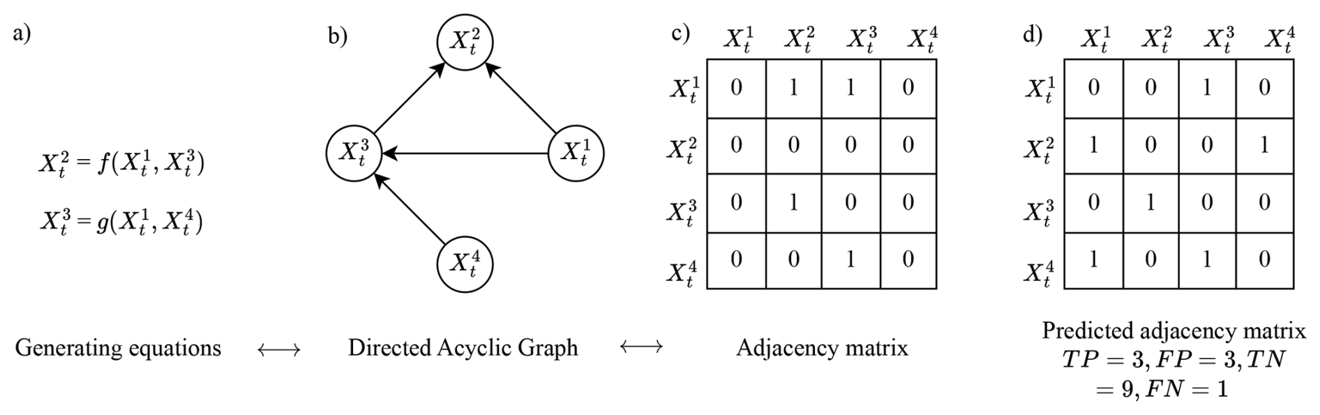
Figure 1Three equivalent methods to describe cause-effect relationship. In (a) variables and are input variables to generate and respectively. This is represented as a graph in (b) with directed edges from nodes into node and from nodes into node . The adjacency matrix in (c) represents this with binary operators in the corresponding cell of two variables, for example the directed edge in (b) between and is shown with “1” in the fourth row (cause) and third column (effect). (d) shows an exemplar adjacency matrix compared and its cells classified, with respect to (c).
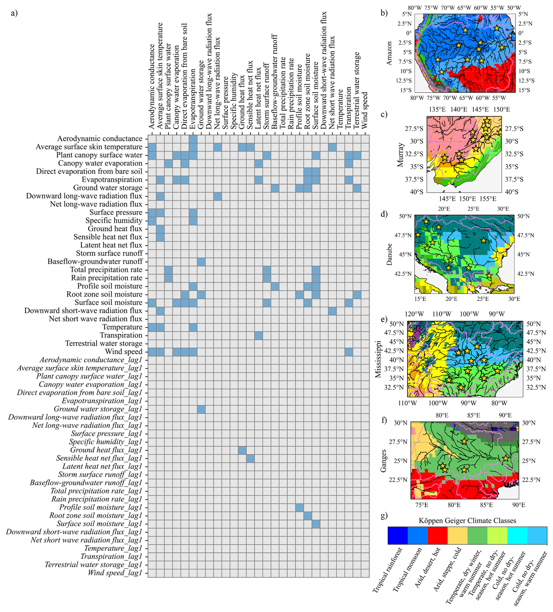
Figure 2(a) The True adjacency matrix representing the causal relationships between the simulated and forcing variables of CLSM-F2.5 model. Similar to Fig. 1c the matrix shows the relationship of causes (row variables) to their effects (column variables). The matrix is created based on the generating equations of the model (Appendix A2) and the definition of adjacency matrix adopted in Sect. 2.2. There are 82 true positives and 1376 true negatives in the matrix. (b) to (f) show the basins and the grids within, where the time-series data of simulated and forcing variables, were selected for the analysis. We extracted data from locations in nine Köppen-Geiger Climate Classes (eight unique classes). These locations are spread across 5 major river basins. For each Köppen-Geiger Climate Class we selected 5 grid points, thus a total of 45 grid points were selected for analysis. Though CLSM does not use a river routing scheme, we overlaid the HydroSHEDS (Lehner et al., 2008) river network to avoid choosing a grid over a stream, and manually selected points without any preference. (g) The legend showing the various Köppen-Geiger Climate Classes.
2.2 DAG and Adjacency Matrix
In a dynamical system, output variables change state through forcing variables applied to the system, and in response to coupling amongst variables, boundary conditions, thresholds and process noise. Consider the simple dynamical system in Fig. 1a where the cause-effect (causal) relation among variables is represented by functional relationships. This causal relationship can be schematised using graphs as well (Fig. 1b). Graphs represent the relations between variables (nodes) using arrows or links (edges). To represent a causal relation with a graph two necessary conditions are required: directed edges and acyclicity. Since causal relations are direct cause-effect relations, a causal graph requires all the edges to be directed. Further, due to temporal ordering of cause-effect relations, a causal graph cannot contain cycles, for example, rainfall and soil moisture are known to form a positive feedback under certain conditions (Guillod et al., 2015; Bui et al., 2023). However, while rain can affect current and future soil moisture states, soil moisture can only affect the future state of rain, not the current or past states. A graph with acyclicity and directed edges is called a Directed Acyclic Graph or DAG (Fig. 1b). DAGs are a common representation of causal relations (Pearl, 2009; Peters et al., 2017).
A DAG can also be represented as a matrix, called an Adjacency Matrix (Fig. 1c) (Peters et al., 2017). Representing DAGs as a mathematical object allows various mathematical operations to be performed on it (see Sect. 2.3). An adjacency matrix has its rows (or columns) named after the variables of the system and its columns (or rows) as the transpose of the former. The existence (or non-existence) of a relation between two variables is represented with a binary operator (1 and 0 or true and false) in the corresponding cell of the matrix. To show the directionality of relations, we choose to define the adjacency matrix such that the causes reside in the rows and the effects reside in the columns (see Fig. 1c).
We note that the strength of causal relations can be represented by the coefficients of the adjacency matrix, such that the values lie between . However, in this paper we are only interested in the presence (and absence) of causal relations, thus we restrict the adjacency matrices to represent the same via 1′s and 0′s.
An interesting consequence of causality and acyclicity of DAGs is the lower triangular ordering of the coefficients of the adjacency matrix (Cunningham and Schrijver, 1998; Park and Klabjan, 2017). It can be shown that by following a simple rule given in Eq. (1), the rows ri of an adjacency matrix Aij can be reordered to convert it into a lower triangular matrix.
where → represents a causal relation between variables ai and aj.
The following section discusses some methods to compare the similarity of two causal graphs.
2.3 Performance evaluation metrics
To compare two graphs, i.e. adjacency matrices, say where one represents the reference truth and the other an estimate of truth respectively, we can create a one-to-one correspondence between their coefficients. Thus, with two possible values in corresponding cells of both the matrices, we have four classes of comparison outcomes. As an example, consider matrices (c) and (d) in Fig. 1 as estimated and true adjacency matrices, respectively. Now, if corresponding cells in the true adjacency matrix and the estimated adjacency matrix contain 1, then the cell in the estimated adjacency matrix is a class of True Positive or TP. Similarly if corresponding cells contain 0, the cell is under the True Negative category (TN). If the true and estimated cells contain 0 and 1 respectively, then the cell is termed a False Positive (FP). Similarly, a False Negative class (FN) implies a 1 in the true adjacency matrix and 0 in the estimated adjacency matrix, see Fig. 1d) as an example. Using these classifications, various quantifications of adjacency matrix can be calculated (below).
- a.
Recall. The primary aim of any predictor or causal discovery algorithm is to identify the drivers of a system. Thus we choose Recall (or True Positive Ratio) to evaluate the ability to accurately identify the correct links in the adjacency matrix (Powers, 2020).
- b.
Matthews Correlation Coefficient (MCC). While Recall is a good metric to evaluate performance in identifying the true positives detected by an algorithm, it does not consider the true negatives and false positives classes. As a result, Recall does not consider the imbalance in different classes of the confusion matrix. Such metrics can show a biased picture in cases of high class imbalance (TP ≫ TN or TP ≪ TN). MCC considers all the four classes (TP, TN, FP and FN) and thus is unaffected by any imbalance in the dataset (Chicco and Jurman, 2020). Moreover, by considering both the ability to find true causal relations and eliminating false relations, MCC acts as a metric balancing the ability to find causal drivers and retaining a parsimonious representation.
- c.
False positive ratio (FPR). False positive ratio is defined by the number of False Positives identified as a proportion to True Negatives in the adjacency matrix (Powers, 2020).
2.4 Synthetic model and data
We surveyed various models and their outputs with the following criteria in mind: (a) all data generated by the model are available for use, (b) all model forcing variables are available, (c) all the time-series are available at the same resolution at which they were generated or used, and (d) the model provides a global coverage of land area. With these criteria, we surveyed various models (Gosling et al., 2023; Schellekens et al., 2017) and selected the Global Land Data Assimilation model Version 2.0 (GLDAS) outputs (Li et al., 2018). GLDAS primarily models the natural processes of land surface and sub-surface, with no representation of human activities like irrigation, water resources management practices like dam and canal operations. Other models such as WaterGap, PCRGLOB-WB, H08 etc., simulate such processes, however, their publicly available datasets, did not meet our above criteria.
The GLDAS dataset is a family of outputs from three Land Surface Models, Catchment Land Surface Model (Koster et al., 2000; Ducharne et al., 2000) (CLSM), NOAH-Land Surface Model and the Variable Infiltration Capacity model. We choose the output from the CLSM model. CLSM is based on the Mosaic Land Surface Model (Koster and Suarez, 1992) and adopts its energy and canopy interception routines. The model does not have vertical layers and it adopts the TOPMODEL (Beven and Kirkby, 1979) framework to simulate sub-surface moisture, defined as the average amount of water required to saturate the catchment. The vertical distribution of soil moisture profile is derived within the model framework using the soil hydraulic parameters from the Clapp and Hornberger (1978) model. Snow is represented with a three-layer snow model described in Lynch-Stieglitz (1994).
To create an adjacency matrix from the generating equations of CLSM, we did a literature review of the model structure and equations (Appendix A), and created the True CLSM adjacency matrix (Fig. 2a), following the definitions of a DAG and its corresponding adjacency matrix (explained in Sect. 2.2). Thus, the true adjacency matrix represents only the causal interactions of various state and flux variables, as represented by the model's generating equations, thereby rooting the causality in physical processes only. While a majority of the variables are generated with contemporaneous states, some variables, like storage terms (surface soil moisture storage, root-zone soil moisture, etc.), are dependent on their previous states. These are represented with lagged relations (Fig. 2a). The True CLSM adjacency matrix acts as a reference truth for our analysis, representing the cause-effect relations in the generating equations. We extracted data from eight different Köppen-Geiger Climate zones (Fig. 2b–f) to understand the performance of these methods in different climates. More details regarding the forcing, simulated variables and simulation period are described in Appendix A.
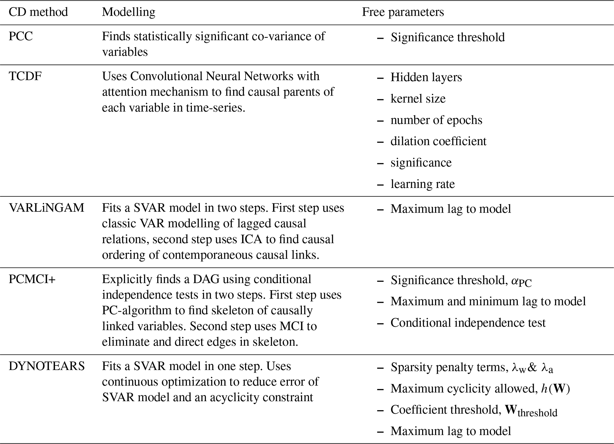
Table 1Table summarising PCC and Causal Discovery algorithms considered for evaluation.
2.5 Methods: Causal Discovery algorithms
Table 1 summarizes the assumptions, modelling framework and free parameters of the various CD methods evaluated here. As mentioned above, each of these methods can be applied to a multivariate time-series dataset to unravel drivers of variables with multiple confounding, self causation, and contemporaneous and lagged causal relations.
These methods adopt theoretically different modelling frameworks, for example, TCDF uses traditional Neural Networks to model time series datasets and uses GC to interpret the attention scores to unravel causal relations in the data. In turn, both VARLiNGAM and DYNOTEARS use traditional Structural Vector Auto-regressive model (SVAR) modelling to find the causal relations in the data. However, they implement different strategies to find the coefficients of the SVAR model. PCMCI+, on the other hand, uses a host of conditional independence testing to find causal drivers of a variable.
For the section below, we consider having time-series data for “d” variables in where for .
2.5.1 Granger causality based: Temporal Causal Discovery Framework
Introduced by Nauta et al. (2019), Temporal Causal Discovery Framework or TCDF identifies causal drivers of variables by combining deep neural network based modelling with a GC-inspired interpretation of model weights. TCDF can be divided into two broad steps. The first step involves identifying the potential causes of each variable by training deep neural networks. The second step uses the structure of the trained model to determine when a discovered causal driver has its effect (lagged and/or instantaneous).
The first step forms the major analysis of TCDF which can be broadly divided into three parts, where for each variable in the data it begins by (a) training a deep neural network model – a Convolutional Neural Network (CNN) to predict it, (b) it uses the attention of the trained model to identify the potential causes. The attention mechanism of a CNN model helps it to focus on certain variables when predicting a target variable, and (c) to verify the potential causes as true causes, it conducts a feature importance step by randomly permuting the values of a potential cause and predicting the target variable. Thus the first step ends by identifying the (likely) true causes of a variable and its corresponding trained CNN model.
In the second step, TCDF determines the temporal order of relation between the identified causes and the target variable. To do this TCDF simply interprets the kernel weights of the trained CNN model. Where TCDF traverses from the output layer (target variable) to the input layer (discovered cause), taking the path with the highest kernel weights. The position where it meets the input layer is decided as the order of the lagged relation. Both steps are repeated for the remaining variables in the system to identify all causal relations in the system. We describe the algorithm below, for a detailed description we suggest reading Nauta et al. (2019).
TCDF begins by training an independent CNN model for each variable. Thus, for each (target) variable Xj (for , it uses an independent CNN, Nj, to model the patterns in its time-series. This network uses all the other variables and their lags and past values of Xj. Thus network Nj is responsible for modelling Xj and its causes. Inside Nj, channels ni (for ), exist, which are responsible for modelling the relation from a variable Xi to Xj. Note that nj models self causation. Next, to identify potential causes of Xj it uses a GC-inspired approach. TCDF considers a variable Xi as a potential cause if it improves the prediction in Nj by reducing the model loss. To identify which variables the Nj considers important, TCDF uses the attention mechanism (attention vector aj Eq. 5) associated with it. These attention vectors are 1×N and their coefficients tell how much attention was paid by Nj, to a certain time-series when predicting Xj.
where is called an attention score, which represents the attention given to Xi by Nj when predicting Xj.
The more attention a variable receives, the more likely it is to be considered a causal influence. Since attention scores take continuous values between [0,1], TCDF applies a threshold to convert them into binary decisions (causal or non-causal) attention. Thus, if ai,j exceeds a certain threshold, Xi is considered a potential cause (Pj) of the jth variable. Finally, to verify if the identified causes are indeed true causes it uses a feature importance method called Permutation Importance Validation Method, we briefly define below.
For each potential cause Xi∈Pj, a new dataset is created by intervening into the system. This is done by randomly permuting the values of Xi to destroy their chronological ordering while keeping the values of other variables the same. The trained CNN model in the previous step is run again using the intervened data and the model loss is compared to the previous scenario where no intervention (via permutation) was done. If the loss is significantly higher after disturbing the values of the potential cause, it is considered to be a true cause (Nauta et al., 2019).
The final step involves determining the temporal order of causal relations between the identified causes in Pj and Xj. For this TCDF simply uses the kernel of the trained CNN model. The kernel is a convolution operator between Xi (the input layer) and its effect Xj (the output layer). Specifically, the kernel is a weight matrix of size N×K, where K is the kernel size. These K weights represent the influence of respective delays on the output. Thus by following the path from the Xj to Xi via the highest weights (coefficients) in the kernel matrix, the position in Xi can be identified which has the maximum influence on Xj. This position is considered to be the lag in the cause-effect relation between Xi→Xj. As mentioned earlier, this entire process is repeated for all the variables in the data to identify causal relations in the system.
As with any deep learning method, TCDF has several hyper-parameters. It requires tuning of a number of hyper-parameters, number of hidden layers, kernel size, number of epochs, learning rate, dilation coefficient and significance (Nauta et al., 2019; Assaad et al., 2022).
2.5.2 Vector Auto-regressive modelling using Non-Gaussian noise: VARLiNGAM
VARLiNGAM, introduced by Hyvärinen et al. (2008), seeks to model the causal relations in time series data with an SVAR model. To find the model coefficients, it uses a classic least squares solution and exploits the lower triangular ordering of the adjacency matrix. Similar to DYNOTEARS, it considers the coefficients matrix as composed of a contemporaneous adjacency matrix and a lagged adjacency matrix. It starts by calculating an initial estimate of the lagged adjacency matrix, this captures the lagged relations in the data. The estimated lagged effects are then subtracted from the original data to get the residuals. Now these residuals are assumed to contain only contemporaneous relations. To find the contemporaneous causal relations in the residuals, it searches for an ordering of the variables such that the resulting matrix is lower triangular, thus representing a DAG. Finally, it uses the contemporaneous adjacency matrix to get the final estimate of the lagged adjacency matrix. Specifically it seeks to model the data with an SVAR model of p lags as:
where Xt is a d×n matrix containing the time series data for all d variables. Bk is a d×d matrix of the causal relations at lag k. is a vector of errors obtained from model inaccuracy. To estimate the coefficients of Bk, it breaks down the matrix into a contemporaneous matrix B0, which contains the instantaneous relations. While Bk for , contains the lagged relations. It begins by calculating an initial estimate, , of the lagged relations , using an ordinary least squares solution. Then it removes the effect of lagged relations from the data to get the residuals as:
these residuals are assumed to contain only contemporaneous relations. To unravel these relationships it uses LiNGAM analysis.
The Linear Non-Gaussian Structural Equation Model or LiNGAM analysis was introduced by Shimizu et al. (2006). LiNGAM allows modelling of causal relations in a vector regressive model (i.e. a SVAR model with no time delays). LiNGAM assumes the causal relationships can be represented via an acyclic adjacency matrix (i.e. a DAG) and that the error terms are mutually independent and non-Gaussian. It exploits the non-Gaussianity, by using Independent Component Analysis (ICA) to find the causal ordering of the contemporaneous relationships (Hyvärinen et al., 2001). To find the coefficients matrix, it searches for an ordering in the columns of the matrix such that the resulting matrix is lower triangular and hence equivalent to a DAG representing causal relations. Note that for a small number of variables this can be done by following the steps in Eq. (1). However, for a large number of variables this becomes computationally expensive. LiNGAM finds this ordering by posing the problem as a classic ICA problem (Hyvärinen et al., 2001). Consider Eq. (7) written as:
where .
The aim is to find a permutation of the matrix W such that it has ones on its diagonals. So that B0 = I - W yields a matrix with zeros on its diagonals, which is a requirement of an adjacency matrix representing a DAG. To do this, ICA yields a raw estimate of , which is then decomposed as = PDW where D is a diagonal matrix and P is the particular permutation matrix which yields ones on the diagonals of DW. Thus we obtain the estimate for the contemporaneous matrix B0. The initial least squares estimate of the lagged adjacency matrix, , is biased as it did not consider the effect of contemporaneous adjacencies. This is corrected once B0 is estimated, which is used to update the estimates of the lagged adjacencies using Eq. (10).
Thus VARLiNGAM has one free parameter, the maximum lag parameter, to control the application of the algorithm.
2.5.3 Constraint-based causal discovery: PCMCI+
The constraint based PCMCI+ algorithm (Runge, 2022) uses conditional independence (CI) tests to find causal parents (drivers) of variables in multi-variate time-series data. It achieves this in two steps, (i) skeleton identification phase using a modified form of PC-alg (PC1), to model lagged relations, and (ii) full skeleton phase using Momentary Conditional Independence tests, to discover contemporaneous relations.
In the first phase PCMCI+ creates a skeleton, i.e. an undirected graph, of all plausible lagged relations. Thus a graph 𝒢 is initialized with all possible edges between pairs of contemporaneous and lagged variables. Then to remove the non-causal relations (edges) it uses CI testing. It uses the PC1 algorithm to reduce the number of CI tests required. Thus it ends with a partially directed graph representing lagged causal relations.
The second phase is designed to identify contemporaneous and self causation. It begins by re-initializing the graph 𝒢 obtained at the end of the first phase. Once again CI tests are used to remove non-causal edges. Here it uses Momentary Conditional Independence tests, which unlike PC1, also considers contemporaneous and self causation (Runge et al., 2019a). Additionally, collider orientation and rule orientation phase are used to orient any un-oriented contemporaneous or ambiguous links. Thus, it ends with a DAG likely representing the underlying causal relations in the data. We briefly explain the algorithm below.
The skeleton identification phase begins by creating a skeleton of all possible lagged relations. Here it starts with a fully connected undirected graph, 𝒢, with edges between all pairs of contemporaneous variables and their lagged versions (up-to the maximum anticipated lag, p). Such that for a particular variable , all possible (lagged) parents are considered. Let the set of plausible parents for be , where .
Now, it tests for CI between and one of its plausible parents from , say , by conditioning them against the remaining parents, if the hypothesis, Eq. (11), is not rejected at a desired significance level αPC, then the variable is removed from the set of plausible parents (consequently the edge is removed from 𝒢).
For a given size of parent set, say L, a high number of combinations for the conditioning set S can be generated (2L), which is also the problem faced by TE (Runge et al., 2012). This makes the task of pruning edges with CI tests computationally expensive, while a large conditioning set reduces the strength of the CI tests (Runge et al., 2019b). As mentioned earlier, PCMCI+ uses a modified form of the PC-alg, PC1, to reduce the number of CI tests required. The algorithm starts with the smallest possible conditioning set (τ=0, where ) and iteratively increases its size until the parents in are exhausted in the conditioning set, i.e. all possible parents of form the conditioning set S (). Thus by prioritizing smaller conditioning sets in the CI tests, it reduces the size of and also preserves the strength of CI tests with smaller size of the conditioning set S (Runge et al., 2012).
Now, within each pth iteration, the conditioning set can have different variables and their combinations as the conditioning set. This can quickly lead to an extremely high number of CI tests to be performed. For example, if and τ=3, the number of CI tests performed would be 8C3. To avoid this, the algorithm tests only against the strongest p combinations of the conditional set. Therefore for τ=0, the conditioning set is empty and the CI test is equivalent to a correlation analysis. The algorithm sorts the parent set according to the strength of correlation in the previous step. For τ=1, the CI test is equivalent to a partial correlation analysis, and so on. Where it tests for CI using only the first (strongest correlated) variable from in the conditioning set S.
To deal with auto-correlation in the time series and find the contemporaneous links, authors use the Momentary Conditional Information test (MCI) (Runge, 2022). The main difference between PC1 CI test and MCI test is that the latter considers the causal parents of the variables undergoing the CI test in the conditioning set itself (Eq. 12) (Runge et al., 2019a). Thus in the second step, the graph 𝒢 is re-initialised by adding all the contemporaneous links possible. Now, similar to PC1, pruning and orientation of edges follows using the MCI test (Eq. 13).
and are the causal parents of and respectively, identified at the end of PC1. S is a subset of contemporaneous adjacencies of . Finally, any undirected contemporaneous edges in 𝒢 are oriented using PC-alg's orientation rules (Spirtes and Glymour, 1991). Amongst the CD methods discussed here, PCMCI+ offers the highest flexibility to adapt the algorithm for discovery in linear and non-linear time-series datasets. Thus it has several free parameters, starting with the significance level of the CI tests in both the PC1 and MCI tests (αPC), second it allows the use of any linear or non-linear (user defined) test for independence in both the stages (PC1 and MCI). Third, the maximum and minimum lag up-to which the lagged relations are anticipated.
2.5.4 Score-based structure learning: DYNOTEARS
Introduced by Pamfil et al. (2020), DYNOTEARS seeks to find causal relations in time-series data by combining classic SVAR modelling with the acyclic property of DAGs. It models the relationships among the variables with an SVAR model and estimates its coefficients by minimizing a loss function. To ensure these coefficients represent only causal relations, DYNOTEARS considers the coefficient matrix as an adjacency matrix. Since an adjacency matrix has to be acyclic by definition, it exploits this by introducing a new term in the loss function. This new loss term represents the cyclicity of the adjacency matrix. Thus, by simultaneously minimizing the loss of fit of the SVAR model and penalizing its cyclicity, DYNOTEARS models the relations in the data and ensures the relations are strictly causal.
Specifically, it finds the coefficients of an SVAR model with p lags:
where W is a d×d matrix containing the coefficients that capture contemporaneous relations among the variables. Thus it is equivalent to an adjacency matrix with only contemporaneous rows and columns (). Similarly, the matrices contain the coefficients that reflect the lagged relationships between variables. Thus, it is equivalent to an adjacency matrix which represents lagged relations, hence it has both contemporaneous and lagged variables in its rows and columns but entries only in the lagged variables rows.
Further Eq. (14) can be rewritten as Eq. (15) such that X is an n×d matrix with each row containing , while are its lagged versions. This can be further compacted such that all lagged relations are represented by and contemporaneous relations by W (Eq. 16). Note that since A contains only lagged relations, it only connects earlier time-steps to later ones and is inherently acyclic due to time ordering (Fig. 1b).
DYNOTEARS estimates the coefficients of the SVAR model, W and A, using continuous optimization to reduce the error of fit. The loss function F(W,A), contains four terms (Eq. 17):
The first term is the sum of square of errors (ℓ2 norm) to reduce the error of fit. Next, since the causal relations in real world data are expected to be sparse, i.e. only a few variables affect a particular variable, thus many coefficients in W and A are expected to be zeros. To encourage this sparsity, a penalty term is added to reduce the number of non-zero coefficients. This penalty is based on the ℓ1 norm – the sum of the absolute coefficients of a matrix. This penalty term is added for both the matrices and weighted with a tuning parameter to control the degree of sparsity: λW∥W∥1 and λA∥A∥1. Finally, to represent causal relations, the matrices W and A must be acyclic. As discussed earlier, A is inherently acyclic. To enforce acyclicity of W, a term is introduced in the loss function to penalize cyclicity in W. Here the cyclicity of a matrix W is expressed as a mathematical function as:
where:
-
tr is the trace of a matrix (the sum of its diagonal entries),
-
∘ denotes the Hadamard product (element-wise matrix multiplication),
-
and d is the number of variables.
This function equals zero if and only if W is acyclic. Intuitively it provides a mathematical formulation of cyclicity, as a continuous function, which can be minimized by an optimization scheme. As suggested by Zheng et al. (2018), the equality in Eq. (18) can be solved using the augmented Lagrangian method. The resulting loss function takes the form as Eq. (17) which can be solved using standard optimization solvers like L-BFGS-B (Limited-memory Broyden, Fletcher, Goldfarb, and Shannon optimization method with bound constraints, Byrd et al., 1995). Finally, since the causal relations are represented by coefficients of the SVAR model, some coefficients can be very small. To ignore such coefficients, the algorithm allows a user defined threshold, Wthreshold, so that only coefficients greater than this threshold represent a causal relation. Thus, DYNOTEARS offers five free parameters to control the algorithm. The two sparsity penalty terms λw, λa, the maximum cyclicity allowed h(W), the threshold of SVAR coefficients Wthreshold, and the maximum lag to search for.
2.5.5 Other methods for Causal Discovery
We note that other distinct methods of discovering causal relations do exist for example, based on difference equations, which represents all causal relations by means of difference equations driving changes in the system (Voortman et al., 2010). Further, based on non-linear state space reconstruction – CCM (Sugihara et al., 2012), etc. For a comprehensive review we suggest reading Assaad et al. (2022); Gong et al. (2024); Ali et al. (2024). As mentioned earlier, CCM has been successfully applied to discover causal relations in hydrological systems. However, we did not select it for evaluation due to two major issues. First, being a bi-variate method, it allows to determine causality only between a pair of variables, thus it is highly susceptible to identify incorrect causal relations in multi-variate system as discussed earlier (Ombadi et al., 2020). Second, more importantly it assumes a deterministic system in order to create the high dimensional manifold which represents the dynamical and thus consistent (causal) relations in the data (Sugihara et al., 2012). In hydrology, observational and process noise are typical in observations. As shown by Ombadi et al. (2020), applying CCM in such systems can lead to reduced power of detecting causal relations. Despite these, it remains a strong candidate for discovering causal relations, when the assumptions are satisfied.
The choice of free parameters for the four CD methods described above was based on the suggestions from their respective papers. Details of these settings, along with those for the PCC method, are provided in Appendix B. In the next section we discuss the set of assumptions adopted by CD methods in order to discover causal relations.
2.5.6 Assumptions
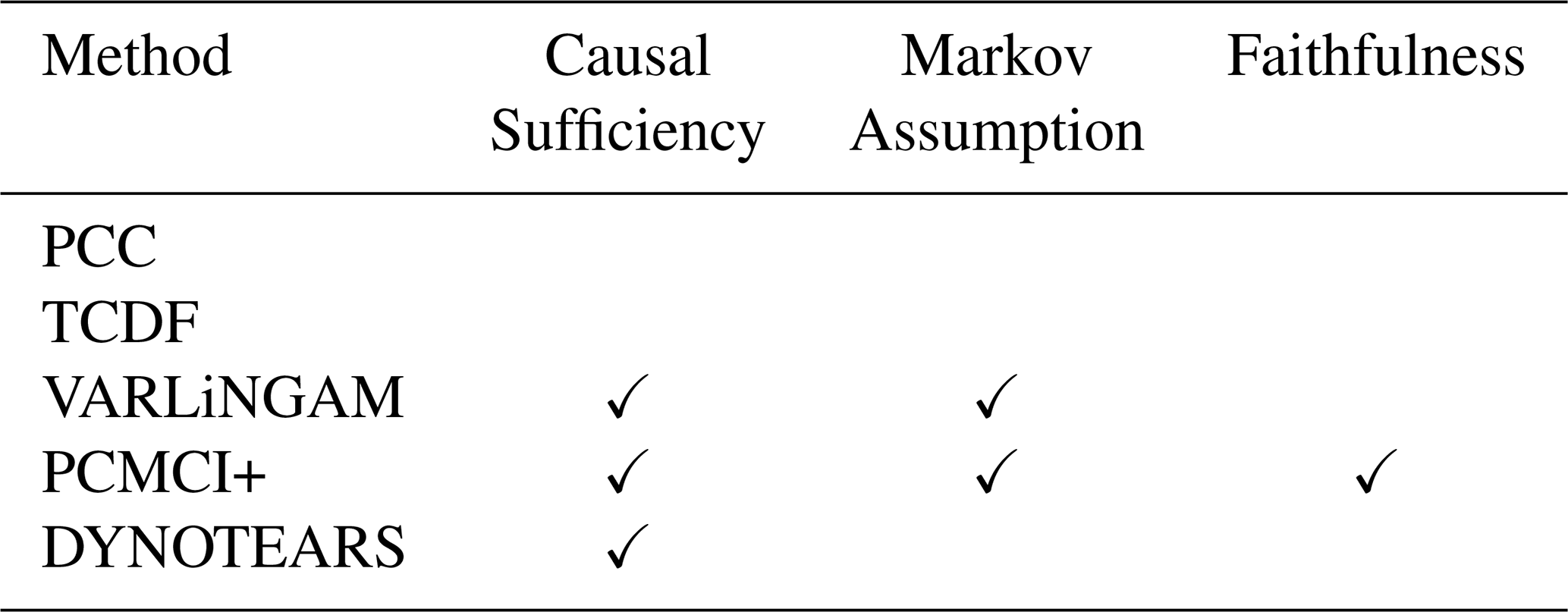
The ability of CD methods to discern causality from correlation lies in the statistical measures used by them and the definition of dependence adopted by them – via DAGs. These rely on two sets of assumptions: one about the nature of the data and the other on the recoverability of the underlying DAG. Thus, assumptions of Gaussian distribution of variables and stationarity of time-series are common to each method, except VARLiNGAM. Assumptions related to the recovery of the underlying DAG are (a) Causal Sufficiency, (b) Markov Assumption, and (c) Faithfulness, (Assaad et al., 2022). Below we briefly define these DAG related assumptions, while Table 2 lists the algorithms which adopt them.
Table 2Causal discovery assumptions. An empty cell indicates the assumption is not needed.
Causal Sufficiency, requires that all the variables which are anticipated to affect the system be included in the analysis. For example, if root zone soil moisture acts as a causal driver of surface soil moisture and transpiration, but it is unobserved, a causal analysis would wrongly yield a causal link between the latter two. Such cases of unobserved variables also result in discovery of incorrect lagged links (Runge, 2018).
Markov assumption implies that a DAG is supported by the conditional independencies present in it. More formally, for the joint distribution of variables in X with Graph G, the causal structure in G is supported by corresponding conditional independence tests. For example, the structure in graph G, Eq. (19), with only two links into Transpiration. The Markov assumption implies that this graph is supported by the conditional independence tests in Eq. (20).
where Pa(Transpirationt) is the Causal parent set of Transpirationt and consists of Precipitationt and Root Zone-Soil moisturet.
In contrast to the Markov assumption, the Faithfulness assumption implies that all conditional independencies of various disjoint sets in X are represented in the graph G. Thus if we are to find the conditional independence in Eq. (20) to be true, the Faithfulness assumption necessitates it to be represented in the structure G, Eq. (19).
2.6 Methods: Non-causal methods
Pearson's correlation coefficient is a widely used method to measure the co-relation between two variables. It quantifies the strength of the co-relation as the ratio of their covariance to the product of their standard deviations.
To test the statistical significance of the obtained PCC value, a hypothesis test can be performed. To do this, a null hypothesis of zero correlation, i.e. no linear dependence between the data is assumed, a significance level α is selected and the p value associated to the PCC value is calculated. α denotes the probability of rejecting the null hypothesis when in fact it is true. The p value is the probability of obtaining a PCC value equal to that obtained, under the assumption that the null hypothesis is true. Thus, if the p value is less than α, the hypothesis is rejected and the obtained PCC value is considered statistically significant at significance level α. For identifying the drivers of a target variable, we found its Pearson’s correlation coefficient with all the remaining variables in the system, both at contemporaneous time step and by creating their one-step-lagged time-series.
2.7 Time-series prediction model
To understand the effect of identifying various drivers (causal and non-causal) of a variable, we evaluated the difference in predicted surface soil moisture time-series when using drivers identified by PCC and the CD methods. In recent times causal discovery has been used in four different ways for time-series predictions. First, Yuan et al. (2022), used the difference in cross entropy amongst observed and simulated variables as a loss function in addition to the sum of square of errors, to train a deep learning model for predicting wetland methane emissions. Second, Li et al. (2022) used the adjacency matrix both, as a feature selection step and to modify the gates of their LSTM cell for soil moisture prediction. Third, Wu et al. (2025) used the adjacency matrix to introduce a causal inference unit alongside the LSTM cell, in their spatiotemporal soil moisture estimation model. Fourth, Vázquez-Patiño et al. (2022) used causal discovery to identify robust features for spatial downscaling of precipitation. Similarly, Zou et al. (2023) used causal discovery to identify the drivers of irrigation water use, to build a prediction model.
Similar to Zou et al. (2023), we use PCC and CD methods to identify the predictors of surface soil moisture. Then, we train machine learning models, based on these sets of predictors. To evaluate the performance of these ML models under contrasting conditions, we selected a location and period which underwent a significant change in climatic conditions. Thus, we choose a grid location in the Ganga basin which exhibited normal conditions between 2000 and 2003 but suffered drought during the 2004–2005 period. Hence, we trained the model with CLSM data from 1 January 2000 to 31 December 2003. While we evaluate their performance during the drought period from 1 January 2004 to 31 December 2005. Furthermore, we conducted a similar exercise for storm surface runoff prediction in Ganga basin and transpiration prediction in the Murray basin, and obtained similar results (Appendix C).
Since model training and evaluation is done using the CLSM data, the models will achieve a near perfect fit irrespective of the number of causal and non-causal predictors identified, or the model structure (Appendix C). This is a result of the perfect model environment, without observational or process noise in the simulated data. Thus, we introduced random additive Gaussian noise to the data to relax this idealized environment. This prevented trivial model fits within a deterministic environment and allowed us to test the models under a representation of observational noise, typically present in hydrometeorological systems. To evaluate the sensitivity of results to the magnitude and realization of the added noise, we conducted Monte Carlo simulations across multiple noise levels (Appendix C).
Further, we adopted two more strategies for evaluating models based on PCC and CD methods. First, we tested the ability of various ML models trained on different sample sizes to understand the effect of training data availability on the performance of ML models driven by causal and PCC based predictors. Second, we tested the effect of dimensionality on the performance of ML models. Since the number of predictors identified by PCC and CD methods are different, we selected a consistent number of predictors across all methods. This allowed us to test their performance under the same dimensionality. The details of these two analyses are presented in Appendix D and E respectively.
To evaluate the performance of the CD methods relative to PCC, we adopt two broad approaches. First, we see the performance at the macro scale by evaluating the adjacency matrices. Second, we zoom into the analysis by focusing on the drivers of surface soil moisture identified by different methods across all the grid points. Finally, to understand the consequence of finding causal and non-causal drivers in terms of applications, we use machine learning models to predict the surface soil moisture time-series. These models are trained separately with predictors identified by PCC and CD methods.
3.1 RQ1: Can CD methods identify the true drivers in a complex simulated hydro-meteorological system across different climate types?
The primary aim of any predictor discovery algorithm is to identify the true drivers of the target variable. To evaluate this, we consider the Recall (or True Positive Ratio, TPR) of all algorithms across the Köppen-Geiger climate classes in Fig. 3a.
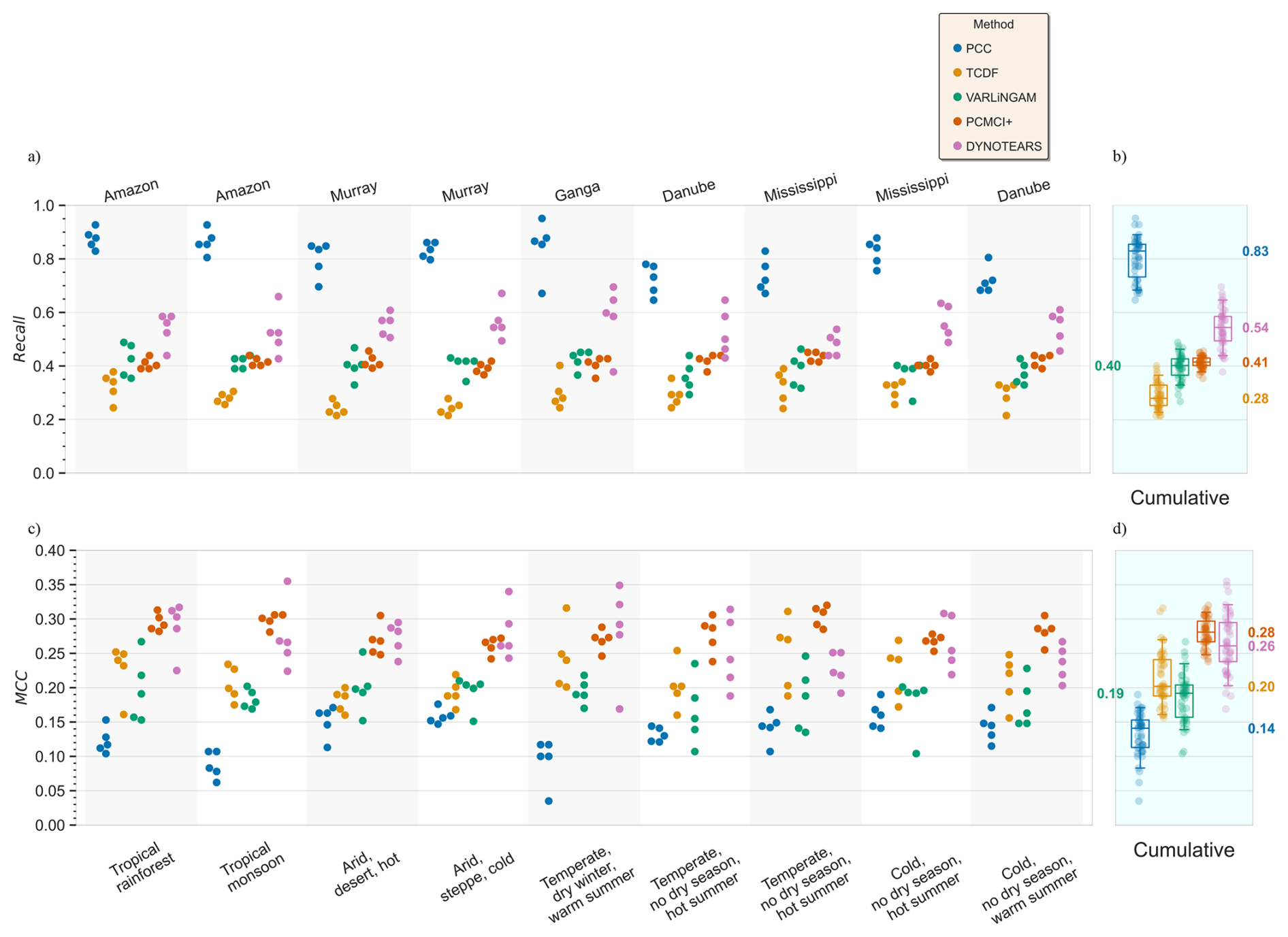
Figure 3Recall (or true positive ratio) (a) and Matthews Correlation Coefficient (b) for all the algorithms, across different Köppen-Geiger climate classes and in different river basins. The right most boxplots show the cumulative distributions with the median values annotated on the y axis. Note that both the top and bottom labels are common to (a) and (b). The legend is common to (a), (b). Recall is simply the ratio of true positives identified to the actual number of true positives in the reference truth, , . MCC consider the class imbalance by using all four classes, , .
Overall, across the Köppen-Geiger climate classes, PCC identifies the highest number of links present in the true adjacency matrix (Fig. 2a). While DYNOTEARS shows lower Recall than PCC, the other CD algorithms identify half or fewer causal links. The cumulative plot indicates that PCC exhibits the largest inter-quartile range (IQR). While CD methods show a narrower IQR, in the order PCMCI+ < VARLiNGAM < TCDF < DYNOTEARS. Interestingly, TCDF, VARLiNGAM and PCMCI+, have Recall scores strongly bound between (0.2–0.5). This is not expected as all three algorithms have different assumptions and adopt different methods to find true drivers.
Amongst the climate types, the temperate climate type exhibited the highest variability in results across methods. For example, PCC shows highest variance within the Ganga basin. Similarly, TCDF shows the highest variability in Mississippi basin, VARLiNGAM in Danube basin and DYNOTEARS in Ganga basin. While PCMCI+ remains relatively stable across all climate types. Overall, CD methods show a relatively stable Recall across climate types.
3.2 RQ2: What is the overall performance, in terms of identifying causal relations and eliminating non-causal co-relations across different climate types?
As mentioned in Methods, Recall does not consider the other classes of (mis)identification, such as false positives, nor the imbalance in their size. This is especially relevant to our analysis since the True adjacency Matrix is negatively imbalanced with 90 % negatives (1376 negatives and 82 positives). Thus, we use Matthew's correlation coefficient (MCC) score to get a balanced understanding of performances. After considering the class imbalance, we observe a change in the relative performance of all the algorithms (Fig. 3b). We explore these differences below.
The cumulative plot indicates that PCC has the lowest MCC scores, with median MCC 0.14. While CD methods score a median MCC greater than or equal to 0.19. Although PCC has the highest Recall, it has very high false positives, resulting in a lower MCC. Among CD methods, TCDF and VARLiNGAM yield comparable median MCC values, but TCDF achieves higher MCC within the IQR. Similar to Recall results, PCMCI+ achieves the most stable MCC scores, while DYNOTEARS shows the largest IQR amongst all the CD methods. The variability of IQR among CD methods follows the order PCMCI+ < VARLiNGAM < TCDF < DYNOTEARS.
Across the climate types, the temperate climate type produces the highest IQR for all the methods. Specifically, this occurs in the Ganga basin for PCC, TCDF, and DYNOTEARS, and in the Danube basin for VARLiNGAM and PCMCI+. In contrast, the two Arid climate types in the Murray basin produce the only climate where some clustering of MCC values is present across all methods. Overall, for all methods we observe a very high variance in MCC values, both across climate types and within the same climate class or even within the same basin.
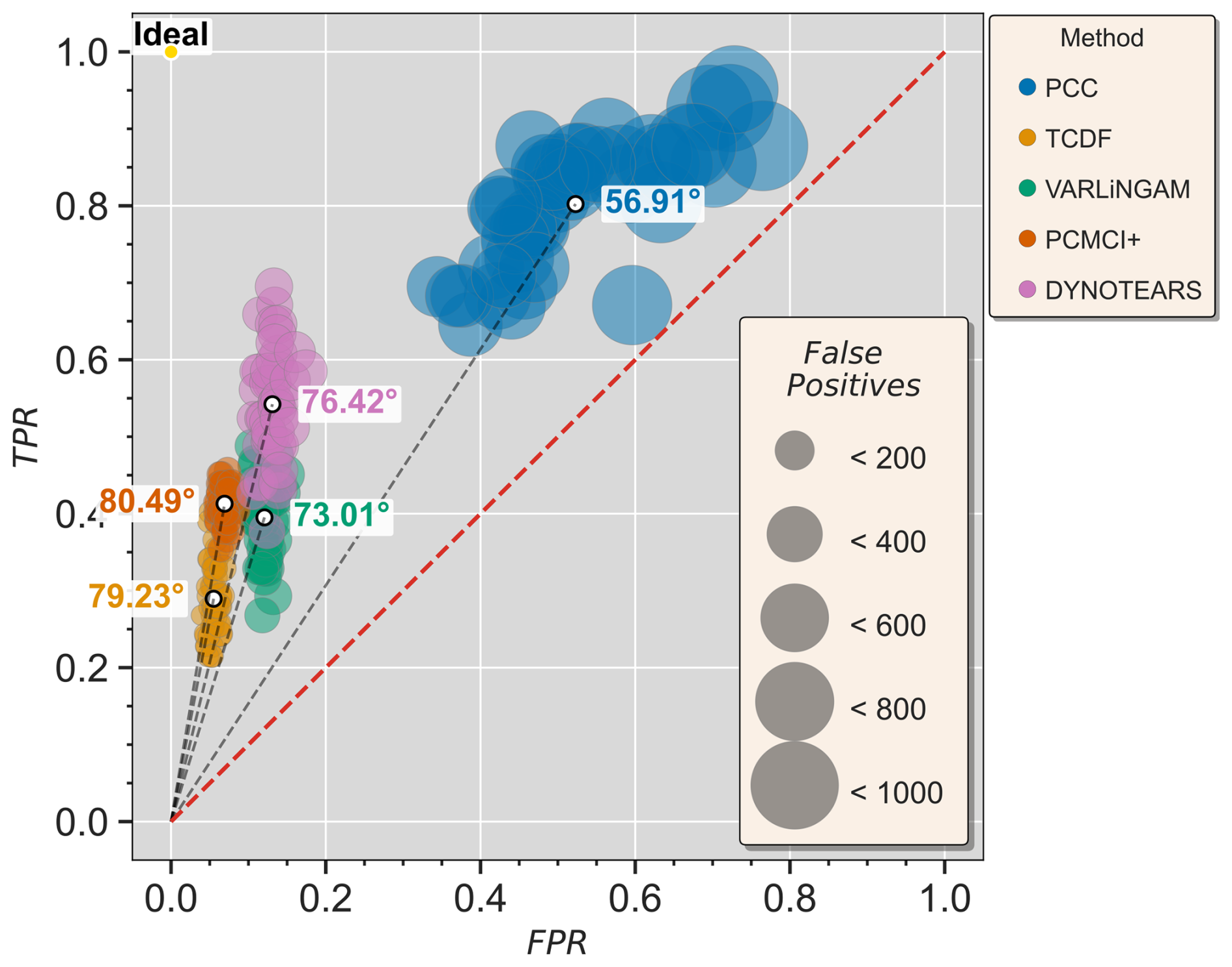
Figure 4Scatter plot of True Positive Ratio and False Positive Ratio in all the grids. The size of the points shows the absolute number of false positives categorically via the False Positives legend. The red dotted line represents a case where TPR=FPR, the top left `Ideal' point denotes a perfect scenario where no False positives are detected and all true positives are identified. The angles in-set show the angle between an imaginary line from the origin to the median of each point cloud and the FPR axes ().
3.3 RQ3: What is the trade off between choosing a correlation-based approach and CD methods?
To better understand the balance between True Positive discovery (Recall) and False Positive discovery we plot them in Fig. 4 for each method. As seen in the plot, the cost of identifying causal links is the accumulation of false positives. Overall, all the algorithms achieve a higher TPR compared to FPR (they sit above the red dotted line, which represents TPR = FPR). Amongst the CD methods, DYNOTEARS achieves the highest TPR, but also suffers from the highest FPR. Further, CD methods show variance along the TPR axis but less variance along the FPR axis. This demonstrates their robustness towards eliminating false positives. PCC shows high variance along both axes, lacking robustness in identifying true positives and avoiding false positives. In terms of absolute number of false positives, CD methods identify less than 200 links incorrectly, whereas PCC identifies between 600 to 1000 incorrect links as true positives. Overall, across the methods, we observe a higher TPR entails a higher False Positive discovery. Since the range of TPR and FPR is significantly different across the methods, we calculated the ratio of TPR to FPR for each method. That is the angle between an imaginary line connecting the origin to the median point of each point cloud, and the FPR axes (Fig. 4). It can be clearly observed that the CD methods, compared to PCC, achieve a higher TPR gain for a unit increase in FPR and a larger deviation from the TPR=FPR line.
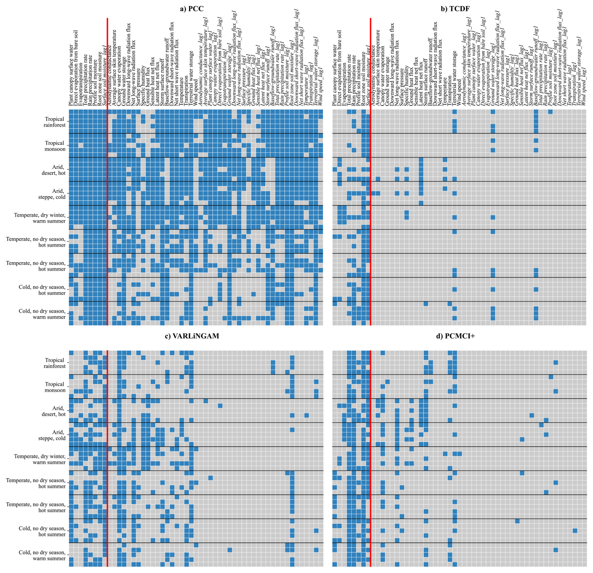
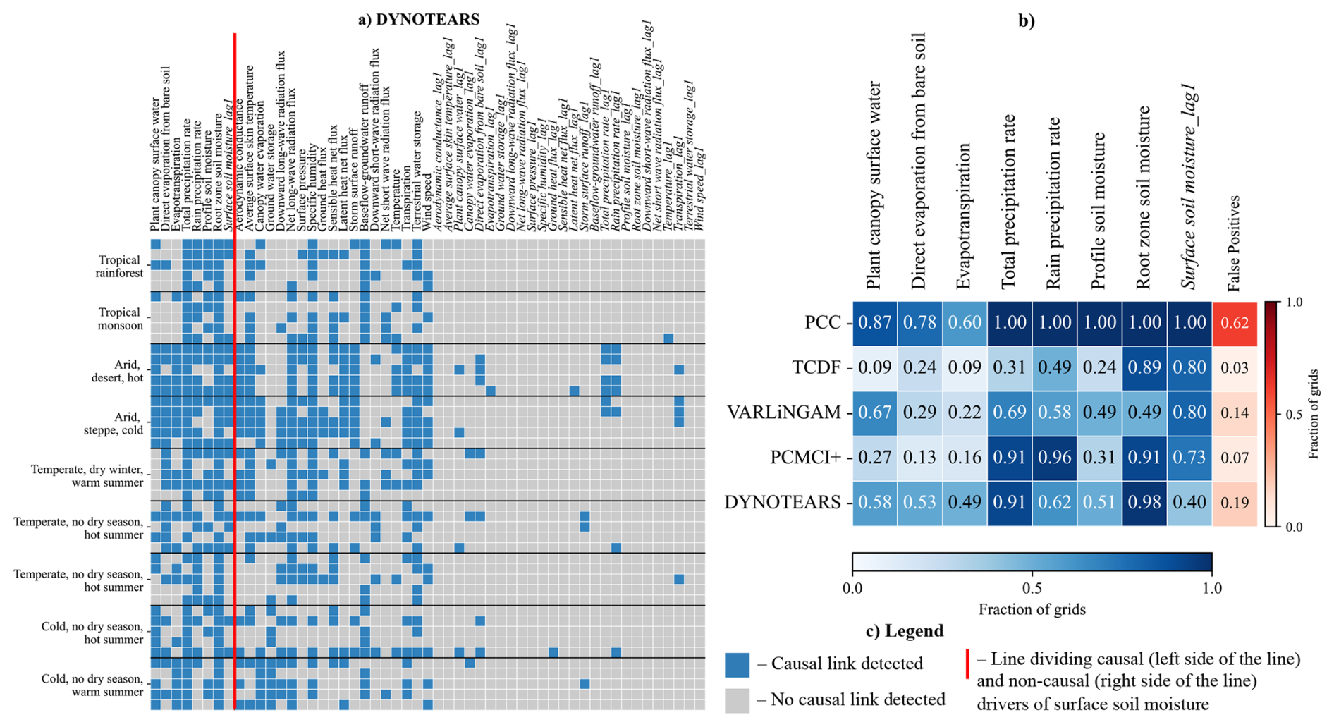
Figure 5Panels (a)–(d) show the various causal drivers of Surface soil moisture as identified by the algorithms in each grid across different climates. The variables left of the solid red line are the causal parents, of surface soil moisture, extracted from the True adjacency matrix, Fig. 2a. Whereas the variables to the right are all the remaining variables of the system and their lags. A blue coloured cell indicates the algorithm has identified a causal link to surface soil moisture from the corresponding variable (column) in the given climate grid (row). Similarly, a grey coloured cell indicates no causal link detected. Note: the legend in Fig. 6c is common to both, Figs. 5 and 6.
3.4 RQ4: Can CD methods help building parsimonious and robust hydrological models?
The previous results sections reported results across all causal relationships within the CLSM model. However, to better understand what the variance in FPR and TPR means in practice, we extract all the drivers of an individual variable, surface soil moisture, identified by the algorithms across all the grids in each climate and plot them in Figs. 5 and 6. Surface soil moisture is an important hydro-meteorological variable as it links the atmosphere with terrestrial hydrology (Seneviratne et al., 2010). In nature, the soil surface stores moisture from the atmosphere and provides moisture back to the atmosphere via evaporation. Active research is ongoing to understand the causality and timescales of this feedback system (Tuttle and Salvucci, 2017; Chauhan et al., 2023; Devanand et al., 2018).
In the CLSM model, surface soil moisture is modelled by combining various modelling routines. We define it explicitly in Appendix A. Essentially, it is modelled as a reservoir of moisture. The initial value of surface soil moisture is based on the catchment deficit (from full saturation), profile soil moisture. It receives input flux from above ground as excess precipitation and from below the ground as excess root zone soil moisture. While outgoing fluxes are direct evaporation from soil and infiltration into the root zone. To update its state at a time instant, the CLSM model takes the summation of these fluxes and adds (or subtracts) from the storage at the previous time-step. Thus, eight variables form the causal parents of surface soil moisture. These are (i) profile soil moisture, (ii) canopy interception and (iii) total precipitation (iv) precipitation as rain (v) total evaporation (vi) evaporation from bare soil (vii) root zone soil moisture, and (viii) surface soil moisture at the previous time step. These eight causal drivers can be classified into physical mechanisms governing the water and energy budgets. Where direct evaporation from bare soil and evapotranspiration form the energy budget related causal drivers. While plant canopy surface water, total and rain precipitation rate, profile soil moisture, root zone soil moisture and lagged surface soil moisture form the water budget related mechanisms. Below we evaluate the ability of the algorithms to identify the water and energy budget related causal drivers of surface soil moisture and to eliminate the non-causal drivers in each grid of the different climates.
3.4.1 PCC
Causal drivers
Among the water budget related causal drivers, PCC identifies almost all the causal drivers correctly (Fig. 5a), while missing plant canopy surface water in Temperate and Cold regions. Similarly, it identifies the energy budget related drivers correctly in Tropical, Arid and Temperate, dry winter and warm summer regions. However, it misses them in other Temperate and cold regions. Interestingly, PCC was able to identify canopy surface water as a causal driver. Since the canopy water acts as a reservoir above the surface and allows rainfall to reach the surface only if it is full to its capacity, it adds some non-linearity to the generation of surface soil moisture. Among CD methods, only VARLiNGAM and DYNOTEARS were able to identify this driver in at least half of the grids (Fig. 6b).
Non-causal drivers
PCC also classifies a very large number of non-causal variables as drivers, resulting in large false positives (Fig. 5a). For example, variables such as latent net heat flux, downward short-wave radiation are closely related to surface soil moisture and part of the surface energy budget and are also identified as causal drivers in a majority of the grids. Similarly, water budget variables like storm surface runoff, groundwater storage, are also classified as causal drivers. Though such variables may have a direct impact on surface soil moisture in the natural environment, these variables are absent in the generating equations of surface soil moisture in the CLSM model. Hence, they do not form the causal parents. Thus, PCC showed a systemic error by identifying many variables as drivers, consistently across different climate classes.
3.4.2 TCDF
Causal drivers
TCDF identified the fewest causal drivers amongst all the methods (Fig. 5b). Only three of the water budget related causal drivers, Rain precipitation rate, root zone soil moisture and lagged surface soil moisture, were identified in about half or more of the grids. While the energy budget related causal drivers could be identified only in some grids of the Temperate, dry winter and warm summer region.
Non-causal drivers
It showed a systematic error by falsely identifying the latent net heat flux as a possible driver in the Arid climates and lagged relation from baseflow in Tropical climates incorrectly (Fig. 5b). Apart from these, no other variable is consistently misidentified. Overall, TCDF achieves the fewest false positives across all climates (false positives = 0.03), making it the most conservative in terms of spurious detection.
3.4.3 VARLiNGAM
Causal drivers
The water budget related causal drivers were identified in half or more of the grids (Fig. 5c). While both energy budget related drivers could be identified only in the Arid, steppe, cold and Temperate, dry winter, warm summer regions. Interestingly, the non-linear causal link from plant canopy surface water was identified in Arid, Temperate and Cold regions with some consistency.
Non-causal drivers
VARLiNGAM also showed systemic bias, by incorrectly identifying canopy water evaporation as a causal driver (Fig. 5c). Further it falsely identified canopy water evaporation in most of the grids. Similarly, it failed to eliminate terrestrial water storage in all climates except arid, and ground heat flux and specific humidity in arid climates. Interestingly, it attributed a lagged causal link between surface soil moisture and root zone soil moisture instead of the true contemporaneous causality. Overall, VARLiNGAM identified a higher number of causal drivers while maintaining a lower false positive count (false positives = 0.14), though it showed systemic error against some variables.
3.4.4 PCMCI+
Causal drivers
Barring plant canopy surface water and profile soil moisture, PCMCI+ identified the remaining water budget related causal drivers with high consistency (≥0.73, Fig. 6b). While it struggled to consistently identify the energy budget related causal drivers in all the climate regions. Once again, plant canopy surface water was identified in some grids of Temperate and Cold regions (Fig. 5d).
Non-causal drivers
PCMCI+ also shows a systemic error by falsely identifying canopy water evaporation, storm surface runoff and terrestrial water storage as causal drivers (Fig. 5d). Compared to VARLiNGAM and DYNOTEARS, PCMCI+ has a very sparse false positive detection, similar to TCDF (false positives = 0.07).
3.4.5 DYNOTEARS
Causal drivers
In strong contrast to other CD methods, DYNOTEARS identifies all the causal drivers, except lagged surface soil moisture, in at least half of the grids. However, it missed the energy budget variables completely in the Tropical regions. Further, the water budget related causal driver, self-causation from surface soil moisture, was missed in most grids of Tropical, Temperate and Cold regions (Fig. 6a). The identification of self-causation in surface soil moisture by DYNOTEARS is far less compared to other CD methods and PCC (Fig. 6 column Surface soil moisture lag1), especially given the strong autocorrelation typically present in storage variables.
Non-causal drivers
DYNOTEARS also showed systemic error, failing to eliminate net long wave radiation flux, average surface skin temperature, baseflow, terrestrial water storage and wind speed (Fig. 6a). Interestingly, it identified the fewest lagged variables as causal drivers. Overall, DYNOTEARS identified more causal drivers of surface soil moisture than the other CD methods while only identifying a few more false positives (=0.19).
To understand the effect of missing a few causal drivers and identifying non-causal ones, we compare the difference by creating prediction models. In the next section, we train machine learning models based on the predictors of surface soil moisture identified by PCC and CD methods and evaluate their performance.
3.5 Predicting time-series using causal knowledge
Below we discuss surface soil moisture predictions under a noise level of 0.5 standard deviation, using a feedforward neural network model.
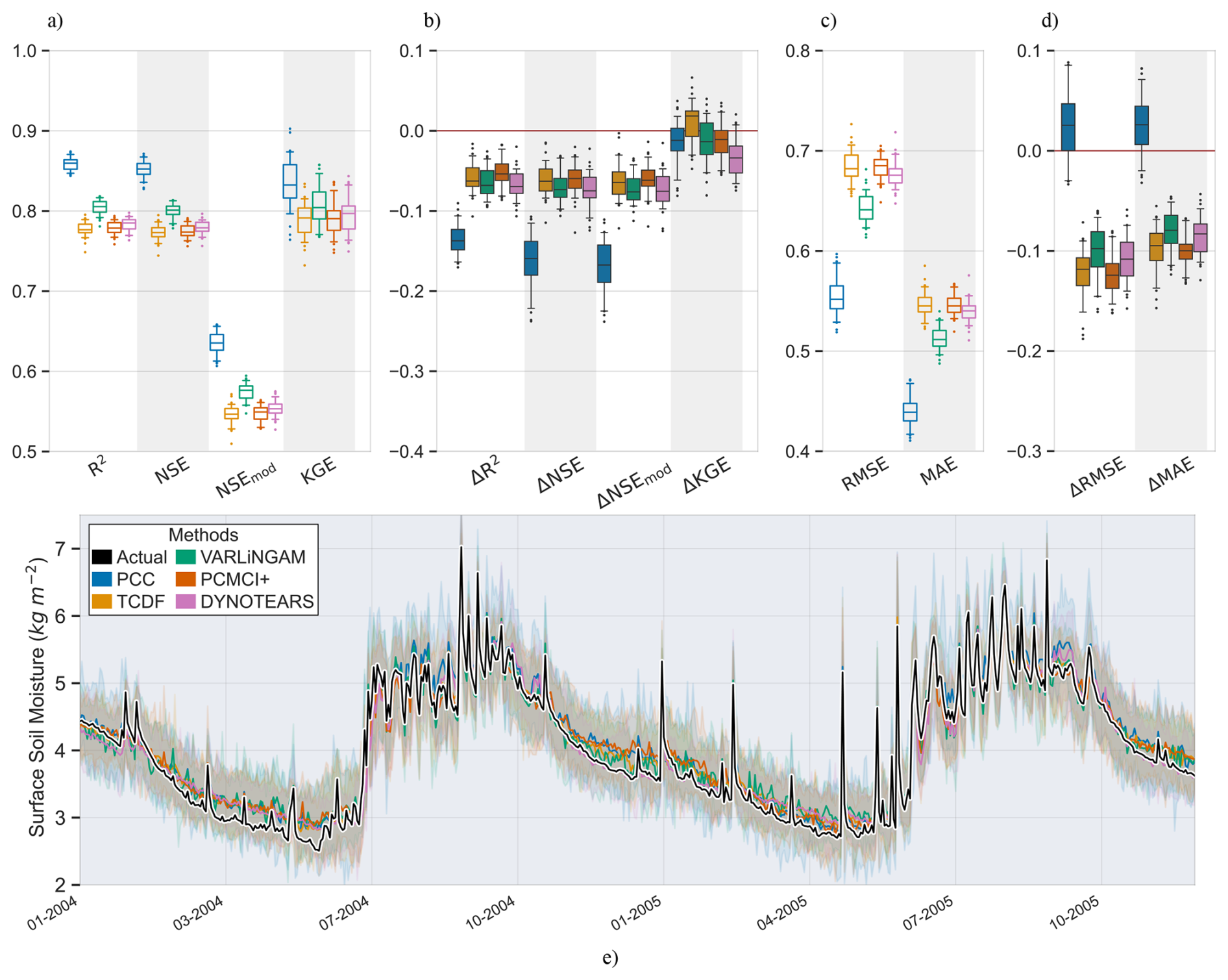
Figure 7Performance and error metrics of the machine learning models created for surface soil moisture prediction. Panels (a) and (c) show the performance and error metrics during the training period. While panels (b) and (d) show the difference in performance and error metrics between the testing and training, e.g.: . Panel (e) shows the predicted and actual time-series in the testing period, based on PCC and CD-based models. For each method, the plot shows the mean prediction of the 100 Monte Carlo simulations, while the shading shows the minimum and maximum range. The metrics adopted are commonly used metrics in hydrology. R2: Coefficient of Determination, NSE: Nash-Sutcliffe efficiency, NSEmod: modified Nash-Sutcliffe efficiency, KGE: Kling-Gupta efficiency, RMSE: Root Mean Square Error and MSE: Mean Squared Error, Jackson et al. (2019). A for performance metrics means a drop in performance during the testing period compared to the training period. While a for error metrics means a drop in performance during the testing period compared to the training period.
In the training period, PCC identified 47 drivers of surface soil moisture, of these 8 were the causal drivers discussed earlier, while 39 were non-causal variables. Similarly, TCDF, VARLiNGAM, PCMCI+ and DYNOTEARS identified 4 causal (4 non-causal), 3 causal (12 non-causal), 6 causal (3 non-causal) and 4 causal (5 non-causal) drivers, respectively. Figure 7a and c show the performance and error metrics respectively during this period. The PCC-based model achieves the highest accuracy relative to its training data, with median R2, NSE>0.8. However, it suffers a sharp decline in performance and gain in error when predicting out of sample during drought conditions. This may be a result of the high number of false positives identified as causal drivers. In contrast, the CD-based models obtain satisfactory performance metrics during the training period with median R2, NSE>0.75, while they show a smaller drop in performance testing out of sample during drought conditions, with median and median . We note that absolute values of soil moisture during the dry years of 2004–2005 are lower compared to the values during the normal years. This resulted in smaller RMSE and MSE values for the CD-based models in the testing period. Both PCC and CD-based models show consistency in performance during the training period with small IQRs. However, during the testing period, CD-based models show higher consistency compared to PCC-based models, with narrower Δ IQRs.
Further, we repeated the above analysis for different levels of added noise, Fig. C2 shows the results. We observe that with increasing levels of noise in the data, the performance of PCC based ML models degrades significantly. While CD-based models show smaller reductions in performance. Figure C1 shows results similar to Fig. C2 but with a different machine learning model, support vector regression. The figure shows similar conclusions, where with increasing levels of noise PCC based models suffer larger reductions in performance compared to CD-based models. Interestingly, at the noise level of one standard deviation, PCC based ML models perform only slightly worse than CD-based models.
Next, the analysis for varying lengths of training sample sizes, Figs. E1 and E2, shows that with shorter periods of training length, all models predict less accurately, but this drop in accuracy stabilises if the training period is longer than a year. Here, CD based models stabilised earlier compared to PCC based models and also suffer a smaller drop in performance across the training and testing periods.
In the analysis comparing various ML models across the same dimensionality of the predictor set, the results show that CD based models have higher performance than the PCC based models, both, in the training and testing periods (Figs. D1, D2). Further, CD based models remain more robust (Fig. D3), and show lower errors compared to PCC based models, both in the training and testing periods (Figs. D1, D2). However, they show similar levels of robustness in the error metrics (Fig. D3).
Overall, PCC-based models identify a large number of predictors and perform better in the training period, but suffered larger performance losses when tested under changing conditions. CD-based models obtain a parsimonious predictor set. This leads to smaller variance in performance during the testing period. More significantly, CD-based models show smaller drop in performance compared to PCC based models, when tested during changing conditions like droughts.
Below we discuss the capabilities of the different algorithms, discuss some caveats to applying Causal Discovery in general and in particular for Hydrology. We close the section with some perspectives on implementing CD methods and discuss limitations of our work.
As discussed in the introduction, Hydro-meteorological systems have highly interconnected variables with strong feedback mechanism and closely related processes. This introduces numerous contemporaneous and lagged correlations in the system. Thus identifying the true causal drivers of a process becomes a challenging task. Thus, a multivariate and cause-effect driven approach is needed to unravel the causal drivers of processes.
By applying multivariate and stochastic framework based causal discovery algorithms, we were able to recover about half of the causal drivers in the system. Further, by considering the possibility of lagged relations in the data CD methods were able to eliminate large numbers of contemporaneous and lagged spurious correlations. This provided a parsimonious set of drivers for different variables, which can potentially lead to better process understanding and identifying the causes of change like streamflow change, droughts etc. However, it also meant CD methods could not detect many causal links in the system.
While Ombadi et al. (2020) applied their CD methods on a simple model forced with stochastically generated rainfall, we evaluated our CD methods on a large, complex model forced with realistic forcings, and evaluated the results across diverse climates and basins of the world. We observed the consistency of CD methods to identify cause-effect relations across these regions. This suggests their viability to be applied in diverse hydrological systems.
Further by focusing on the drivers of surface soil moisture, we found PCC systematically identified large number of correlations with many closely related variables of the energy and water budget, of which a small subset were the causal drivers. This misidentification was consistent as a systemic error, across the different climate regions considered. Whereas CD methods showed such systemic error against far fewer variables, however they missed identifying certain causal drivers of surface soil moisture. A striking feature of CD methods is their ability to correctly eliminate lagged variables as false positives. Whereas PCC classifies each lagged relation of the causal parent as a causal driver. Hence the CD methods are able to handle auto-correlated variables.
To understand the effect of finding causal and non-causal drivers of a variable in terms of time-series prediction, we applied machine learning models to predict surface soil moisture time-series in drought periods. In this regard, we saw (i) CD-based models are more parsimonious compared to PCC-based models, (ii) Both PCC and CD-based models perform good under the training period, (iii) importantly, CD-based models suffer a smaller drop in performance during the evaluation period. This highlights the importance of identifying causal drivers of a process, both for process understanding and predictions, especially under changing conditions like drought and possibly climate change.
4.1 Method specific outcomes
4.1.1 PCC
As we expected, PCC found a high number of co-varying variable pairs. Choosing low threshold of correlation allowed it to discover most of the causal links (median Recall = 0.83). However, the definition of PCC lacks a causal interpretation, thus the variables identified can be called predictors and not causal drivers. This is the reason why any statistical test like PCC, Spearman's rho, Kendall's τ, or measures of Information Flow like Transfer Entropy, Mutual Information etc., are called Variable Selection or Predictor importance step. Overall, and in particular for drivers of surface soil moisture, PCC identifies very high false positives. This creates an illusion of model complexity by including redundant variables and their lags, which are statistically significant but causally unrelated. This makes understanding the process harder, while it necessitates the need of many variables for creating a prediction model that inherently has high computation cost in terms of time and memory.
4.1.2 TCDF
TCDF identified the fewest causal links across all the climates, however it was able to keep false positives to the lowest. As mentioned earlier, for each variable in the system, it uses CNN's to predict it and interprets the attention scores in a Granger-Causality sense to find causal drivers of the variable. The Granger-Causality method was evaluated in Ombadi et al. (2020), though a one-to-one comparison with results from TCDF is unfair, we comment on the similarities and differences we found with the former. Using Granger-Causality Ombadi et al. (2020) reported a high False Positive Rate, even with the small number of variables in their system. This highlights the problem with bivariate methods like PCC, Granger-Causality, etc., in a multivariate system. Where confounding (common cause) and autocorrelation severely affect the false positive discovery (Tuttle and Salvucci, 2017; Ombadi et al., 2020; Delforge et al., 2022). Comparatively, by adopting a multivariate approach and accounting for autocorrelation in its CNN architecture, TCDF was able to reduce the false positive discovery and performed the best (in FPR score) across all algorithms. However, TCDF failed to identify true positives, with the lowest Recall values (median Recall = 0.28). This may result from our inability to sufficiently train the CNN's, since the author's report F1 scores similar to the predecessor of PCMCI+, PCMCI (Nauta et al., 2019). We struggled to improve the Recall of TCDF by tuning its hyper-parameters. The process was particularly difficult owing to its high number of hyper-parameters, typical to any CNN architecture. This maybe since CNN's are better suited to predict spatial patterns and a different deep learning model like LSTM may yield better results (Kratzert et al., 2019).
4.1.3 VARLiNGAM
VARLiNGAM produced one of the most contrasting results amongst the CD methods. It consistently had varying MCC scores in all climate classes. Though it scored Recall values similar to PCMCI+ (median Recall = 0.40), as reported previously (Assaad et al., 2022; Hasan et al., 2024; Runge, 2022). However, it was able to retrieve the non-linear link from plant canopy surface water into surface soil moisture which TCDF and PCMCI+ struggled to retrieve in any climate class. As suggested by Hyvärinen et al. (2008), this may be a result of non-Gaussian errors obtained when VARLiNGAM uses linear models to fit the data.
4.1.4 PCMCI+
PCMCI+ provided the most stable results across all climates in both Recall and MCC scores. Though, on average it could only identify 40 % of all the causal links (medain Recall = 0.41), which is a little lower than reported by Runge (2022). Further, the majority of the causal links in our adjacency matrix (Fig. 2b) are contemporaneous, thus the algorithm was able to retrieve these contemporaneous links, as suggested by Delforge et al. (2022). Ombadi et al. (2020) reported a similar Recall for the base algorithm, PC-alg, for similar lengths of data. This is expected since the dimensionality of our test was higher (4 in former, 27 in ours) and the lag relation up-to which the search was done (lag-1 in former, lag-1 and contemporaneous in ours). However, we obtained similar levels of false positives (FPR <0.2) as Ombadi et al. (2020). This is expected as well, since both the modifications to PC-alg, the skeleton discovery and MCI phase have been designed to handle autocorrelation and contemporaneous edges.
4.1.5 DYNOTEARS
DYNOTEARS retrieved the highest causal links amongst all the CD methods (median Recall = 0.54). It showed that true positives can be discovered from the data as high as PCC, while keeping the False Discovery lower (Fig. 4). The Recall values are comparable to those in Pamfil et al. (2020), however, we obtained a higher False Positive Ratio.
The science of cause-effect analysis has seen rapid development over recent years (Assaad et al., 2022; Gong et al., 2024). Inspired by Ombadi et al. (2020) and the premise of finding causally-related variables, we evaluated state-of-the-art methods of Causal Discovery. While the former evaluated simpler methods of causal discovery in a simple lumped model, in the context of varying length of time-series, process and observational noise, here we evaluated strictly causal methods on output of a large, complex model. This allowed us to test the algorithms over a real-world like system while allowing the generating equations to be used as a benchmark of true causal relationships. We evaluated four theoretically distinct causal discovery methods (TCDF, VARLiNGAM, PCMCI+ and DYNOTEARS) that traverse the broad spectrum of causal discovery methods. We also overviewed some methods of representing causal relations via a graph and an adjacency matrix. By contrasting our results with PCC we exposed how bivariate and non-causal methods lead to inflated drivers.
We found the correlation based method PCC, identified the highest number of causal links, followed by DYNOTEARS. While other CD methods were able to Recall half or fewer causal links. However, CD methods were more effective at eliminating highly correlated but non-causal variables across climate types. By adopting multivariate frameworks with contemporaneous and lagged relations, CD methods were able to identify the correct order of lag relations amongst variables while eliminating multiple spurious correlations. This provided a parsimonious set of causal drivers of a process, potentially leading to a better process understanding and time-series prediction. To test the latter we identified drivers of surface soil moisture during normal conditions with PCC and CD methods, for time-series prediction. Evaluation during drought period showed CD-based machine learning models performed better, with higher performance scores and smaller variability, compared to correlation based models, highlighting the importance of finding causal drivers of a process. Finally, we discussed some caveats to applying CD methods in the real world and discussed how their assumptions and algorithms can be exploited to further retrieve causes of variables in hydrometeorological systems.
5.1 Caveats
It is evident that CD methods are able to identify many correct causal links while eliminating correlated but causally unrelated links. Although useful, satisfying the assumptions of CD methods in the real world can be difficult. For example, certain variables in a hydrological system may not be observed, like soil moisture below the surface, Baseflow, etc. This violates the assumption of causal sufficiency and can lead to spurious links between variables. In such cases, we suggest the identified links should be carefully interpreted in a Granger-Causality sense.
Another consequence of the strict assumptions of CD methods is the need to observe variables at the timescales of their causal interaction. This is especially relevant to hydrological applications since many variables are observed at different temporal resolutions. In such cases, the causal analysis is conducted on temporally aggregated data. Some research suggests partial recovery of the underlying causal interactions while other suggests occurrence of contemporaneous links instead of the lagged interactions (Gong et al., 2017; Runge, 2018).
5.2 Perspectives
In essence, the Causal Discovery methods discussed here are algorithms. Though they provide parameters to tweak their applications, their true potential lies in the fact that they're algorithms and hence parts of their structure can be swapped with alternative modules better suited in the context of their application. For example, as Runge et al. (2019b) and Runge (2022) suggested, if non-linear dependencies between variables are anticipated then the conditional independence tests of PCMCI+ can be done using various linear and non-linear methods. Similarly, if fewer lagged relations are expected in a system, then the initial estimate of the lagged adjacency matrix in VARLiNGAM can be calculated using a sparsity penalty (L1-norm of errors) instead of using a Ordinary Least Squares approach (L2-norm of errors).
Further, as mentioned by the authors of VARLiNGAM, the assumption of non-Gaussian errors makes it a unique tool in the family of Causal Discovery methods. We believe this makes it a valuable tool for CD in climate change scenarios, where non-stationarity in the distribution of hydro-meteorological variables is expected, which yields non-Gaussian model errors.
Although the objective of DYNOTEARS is to find a DAG, its theoretical implementation to find it as coefficients of a SVAR model allows for familiar interpretation. As SVAR models have long been used in Hydrology, particularly in forecasting models as ARMA, ARIMA and similar models. In the case of TCDF, by adopting the Granger-Causality framework, it avoids the fulfilment of the strong assumptions of Causal Sufficiency, Causal Markov assumption and Faithfulness on the data. This theoretically allows it to be applied in systems where the above assumptions cannot be satisfied.
5.3 Limitations
There are several limitations to our work. First, as mentioned by Ombadi et al. (2020), causal interactions can evolve in time and different mechanisms can drive a process in different time periods. For example, they found wind speed as a causal driver of evapotranspiration during the summer season but no causal link was not identified in the winter season. This phenomenon of time-evolution of causal relations has been recognized in the literature and classified as an issue to be addressed when identifying causality in a time window or over the entire time-series (summary causal graph) (Ombadi et al., 2020; Assaad et al., 2022). To this end, we applied causal analysis over the entire time-series, thus focusing on causal interactions over the entire time-period. Second, we assumed stationarity of the time-series data, which is necessary for many statistical tools like Linear Regression, which forms the backbone of most of the methods discussed here. Third, by performing the analysis in a simulated environment we ensured Causal Sufficiency. As discussed above, this may not be possible in real-world applications. This leads to the fourth issue, where the number of variables in the system increases to very high numbers. This creates a problem for algorithms in terms of (i) expanding the number of possible causal links that need to be evaluated (and eliminated if necessary), (ii) convergence of methods and (iii) computational time required. One could argue, for example, in the case of identifying the causal parents of surface soil moisture, that certain variables, like ground water storage, etc, could be excluded from the CD analysis as a direct cause-effect relationship is not expected between the variables. Thus, increasing the detection power of CD methods. Fifth, we applied CD methods in a simulated environment that represents physical processes with through a contemporaneous and 1 d lag relations. In contrast, many real-world hydrological variables, such as soil moisture, groundwater storage, and snowpack, exhibit pronounced long-term memory when observed empirically. In observational datasets, we rarely capture the complete state vector of the environment. This partial observability means that the unmeasured physical delays (e.g., percolation time, routing) manifest statistically as long memory. Therefore, if a purely data-driven modelling framework is to be used for prediction based directly on observations, relying solely on lag-1 variables is often insufficient, and higher-order (multi-step) Markov processes or autoregressive models are required to account for the system's integrated memory. While the CD methods evaluated in the manuscript can be adapted to allow detection of multi-step causal relations in a system, derivation of true drivers in this study is based on the mathematical governing equations of the CLSM F-2.5 model (Appendix A2). Because this simulated environment is governed contemporaneous and 1 d lag transitions, the resulting true causality matrix only contains contemporaneous and 1 d lag relations. Thus, the CD methods were evaluated on their ability to accurately identify the correct causal variable and its correct lag, up-to one timestep. This constraint was an intended design to robustly contrast the key drivers selected from CD against those selected by empirical correlation-based methods, and to evaluate their predictive skills assuming that an exhaustive set of hydrological variables (both forcing and state) is accessible.
However, the limited availability of complete observation data indicates that variables with longer lag need to be considered when applying CD to real-world datasets. Investigating causal structures under these conditions is an interesting topic of future research, as some apparent long-lag causal relationships may actually represent pseudo-causality induced by hidden variables and limited observability. Further studies are warranted to explore scenarios within simulated environments where data availability is artificially restricted to commonly measured variables (e.g. precipitation, discharge and potential evaporation), allowing researchers to determine what can be causally inferred about the missing states. For example, Delforge et al. (2022) utilised CD to reveal hydrological connectivity in a Karst aquifer system using time-series data for rainfall, potential evapotranspiration, resistivity, and percolation rates. By applying CD in both a synthetic case study and real-world observations, they incorporated lag relations of up to five time-steps to accurately capture the time span of preferential flow peaks. Similarly, Abbasizadeh et al. (2025), although with more comprehensive real-world data of climate and catchment attributes, used CD to identify the causal parents (drivers) of runoff signatures and report them to align with existing knowledge of the physical processes generating runoff.
A1 Model description
The CLSM model is composed of various routines to model different processes on the land surface. These routines are adopted or based on other works, Koster et al. (2000); Ducharne et al. (2000). The energy balance and canopy interception schemes are based on the MOSAIC LSM model, Koster and Suarez (1992, 1996). The sub-surface moisture distribution is based on Clapp and Hornberger (1978). Using this distribution, the calculation of sub-surface storages and surface runoff generation is based on TOPMODEL from Beven and Kirkby (1979). Finally, the snow related simulations are based on Lynch-Stieglitz (1994). Since none of the grids selected in our analysis contained any snow variables (time-series was zeros), we do not discuss their governing equations.
The model is forced with nine meteorological forcings from a General Circulation Model. Precipitation, rainfall as fraction of precipitation, downward short-wave radiation flux, downward long-wave radiation, specific humidity, snow precipitation rate, air temperature, surface pressure and wind speed. Since these act as forcing to the model and are not affected by any feedback from it to the GCM, we consider these as independent variables and hence they do not have any causal drivers. Rather, these only act as causal drivers of other variables.
Table A1Table describing the short and long names and units of simulated and forcing variables. * marked variables are forcing variables. Obtained from the GLDAS model documentation (Li et al., 2018).
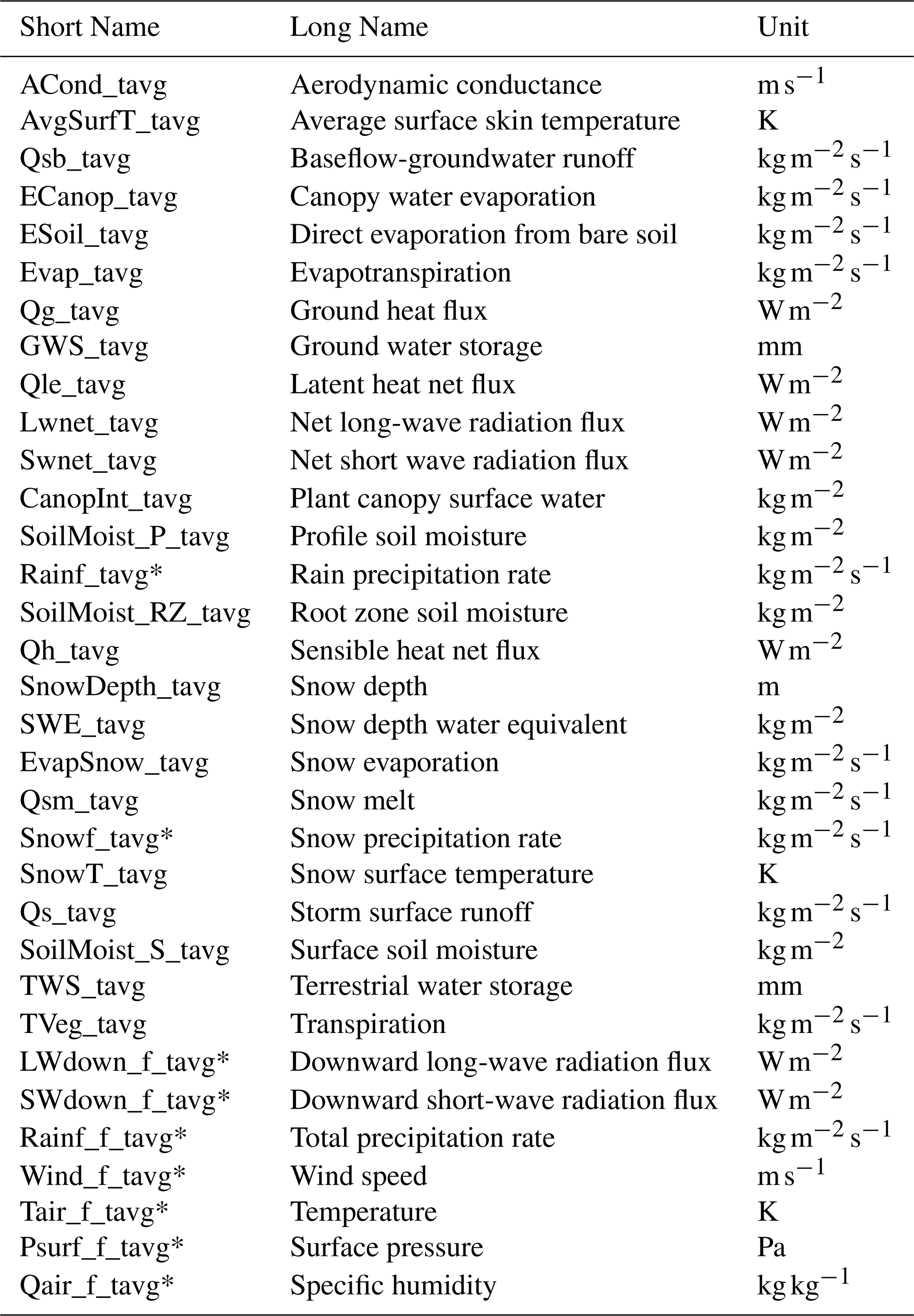
The model simulates various prognostic and internal variables, and outputs 33 hydro-meteorological variables. We avoided snow regions in our analysis due to highly varying snow-related variables where valid data was available. By ignoring the snow related variables we are left with 27 variables listed in Table A1. As mentioned above, eight of these are forcing variables (ignoring snow precipitation rate). Thus, we have a total of 20 dynamically simulated variables in our analysis that have causal drivers.
We found certain differences in the variables described in the original paper and the current version of model outputs. For example the papers describe how a TOPMODEL based bulk variable called Catchment-Deficit is used for sub-surface moisture distribution. However, the current output variables do not contain the same, rather a variable called Profile Soil Moisture is provided. Using visual inspection and literature review we consider Profile Soil Moisture to be the Catchment-Deficit term. Thus we make certain assumptions to overcome such issues wherever necessary to obtain all the governing equations and/or relations.
Further, apart from the forcing variables and dynamically generated variables, the model uses a host of static parameters which characterize the local distribution of vegetation and topography. These parameters affect the simulation of various variables, like vegetation indices affect the scaling of transpiration in zones between completely saturated and wilting zones.
Thus in favour of simplicity, we do not mention the full complexity of the model and only mention model equations and/or describe the simulation routine, with the functional forms used to describe the causal relations amongst the variables, which form the reference truth in Fig. 2a.
A2 Modelling schemes and generating equations
Canopy Interception
The canopy interception reservoir has one incoming flux of precipitation and one outgoing flux of evaporation from it. Thus, it has the functional form:
Surface Runoff
If the canopy interception reservoir is full after a precipitation event, the excess precipitation falls onto the land surface as through-fall precipitation. The model divides each spatial unit tile into three types based on the concurrent surface soil moisture. These are: completely saturated region, region at wilting point and the region between these two. The through-fall precipitation falling on the saturated region is immediately converted into storm surface runoff. While the through-fall precipitation on the latter two regions is scaled according to the surface soil moisture capacity. Thus, storm surface runoff is generated as:
where Mse is the surface excess given by surface soil moisture. This gives the functional form for Storm surface runoff as:
Surface and sub-surface storages
In the CLSM model, surface and sub-surface soil moistures are simulated in two steps combining different modelling techniques. First a bulk catchment term called Catchment Deficit is calculated following Beven and Kirkby (1979). Second, this deficit is distributed across the layers of soil using the formulation in Clapp and Hornberger (1978). Then the local values of these storages are based on the antecedent conditions and the transfer of moisture between the vertical levels. The transfer of moisture from surface to atmosphere follows the equations in Koster and Suarez (1992) and sub-surface transfers are simulated using the TOPMODEL scheme from Beven and Kirkby (1979).
Surface soil moisture. The surface soil moisture is modelled as a reservoir of moisture with incoming flux as precipitation (through-fall or direct) and outgoing flux as infiltration into root-zone soil moisture and evaporation from soil. At each time-step the model reduces the excess (or deficit) in this storage by percolating (or gained via capillary action) a fraction of the storage into the reservoir below. The amount percolated (or gained via capillary action) is proportional to the absolute storage, this adds a auto-correlation type relation in the variable. Thus its functional form is given as:
Root-zone soil moisture. The Root-zone soil moisture is modelled as a reservoir of moisture with incoming flux as moisture from Surface soil moisture and outgoing flux as percolation into groundwater and evaporation from soil. Root-zone soil moisture excess (or deficit) is also reduced as proportional to the absolute value of storage. Thus its functional form is given as:
Profile soil moisture. The Profile soil moisture term was assumed to be related to the Catchment Moisture Deficit term in Koster et al. (2000). Catchment moisture deficit is the moisture required to completely saturate the sub-surface and bring the water table to near the surface. Thus it is updated according to the moisture storages in various sub-surface levels locally and summed over the entire catchment. Thus, its functional form is given as:
Groundwater storage. Finally, the root zone moisture transfers the moisture to the water table in the groundwater. The groundwater acts as a reservoir for groundwater baseflow. Thus it has one incoming flux as percolation from Root-zone soil moisture and outgoing flux as baseflow discharge. Thus its functional form is given as:
Baseflow-groundwater runoff
The discharge from the groundwater storage is modelled as a non-linear function of the bulk catchment moisture deficit, the local water table depth and the mean water table depth of the catchment.
where and are the mean water table depth of the catchment and the local topography, Ks(surface) and ν is the surface-saturated hydraulic conductivity and describes the exponential decay of the saturated hydraulic conductivity with depth. Thus, its functional form is given as:
Terrestrial water storage
Terrestrial water storage was not found to be mentioned in the original or supporting papers. Perhaps it was introduced much later in light of the GRACE mission. However, it has been defined in the product README document. Thus the TWS is defined following the same, with the functional form as:
Evaporative Fluxes
The total evaporation from the surface is modelled using a bulk effective resistance term, reff. It captures the effect of canopy resistance, aerodynamic resistance and bare soil resistance. Thus the total evaporation is given as:
Therefore, its functional form is given as:
Similar to the total evaporation the other evaporative fluxes are calculated as below:
where rbs is the bare soil resistance to evaporation and rc is the canopy resistance to transpiration, function of CanopIntt and WindSpeed-ft. Thus, we obtain the functional relationships as:
Aerodynamic Conductance
Aerodynamic conductance is defined on the data product website, as the measure of how effectively vapour flows through stomata openings, total leaf area and soil surface. It is the inverse of aerodynamic resistance. In the papers the effective aerodynamic resistance is defined as the summation of
Energy Balance equations and Vapour flux equation
The above two equations are simultaneously solved using a first order linearization of terms to get the δTc and ea terms.
These are then used to update the values ground heat flux, sensible heat flux and upward long-wave radiation fluxes as:
This gives a functional form for the temperature of the surface/canopy system and the energy budget terms as:
A3 Model forcings and simulation period
As described above, the model is forced with global meteorological forcing dataset from Princeton University Sheffield et al. (2006). The model simulations were initialized on simulation date 1 January 1948 using soil moisture and other state fields set at climatology. The total simulation period spans 1 January 1948 to 31 December 2014. The models simulates the variables at 3-hourly intervals and provides the output at 3-hourly, daily and monthly temporal resolution. The data used in this study was from 1 January 2002 till 31 December 2014 at daily timescale resolution.
Below we describe the algorithm parameters used and modifications applied for this study. Before running the analysis we standardized the data by subtracting its mean and dividing it by the standard deviation. Since the maximum lag in causal relations was set to be 1, we conducted the analysis by fixing the maximum lag parameters accordingly for testing.
B1 PCC
For PCC, we selected only those variables as drivers where the p value was smaller than 0.05 and absolute correlation coefficient greater than 0.2 (Wu and Chau, 2011) We chose a low correlation threshold to maximize the inclusion of potential causal drivers, while reducing the likelihood of retaining purely spurious associations via the significance threshold.
B2 TCDF
As summarized in Table 1, TCDF has six parameters. By reviewing the method paper, we chose the following parameters: maximum lag = 1, hidden layers = 0, kernel size = 4, dilation coefficient = 4, number of epochs = 1000, significance = 1 and learning rate = 0.005.
B3 PCMCI+
The parameters for PCMCI+ were minimum lag = 0 and maximum lag = 1. In addition, at the significance threshold αpc=0.95, the conditional independence test was the partial correlation (ParCorr) from the tigramite package itself (see Code availability). Since the analysis data was from a perfect environment with no observational or process noise, this could potentially lead to “perfect fitting” of various variables during the conditional independence tests. This leads to variables negating each other's effects, where in fact, both may be causal drivers (Ombadi et al., 2020). This is a case of violation of causal faithfulness, wherein the causal relations exist, however they cannot be recovered by conditional independence tests (Runge, 2022). Thus, to avoid such issues, we added randomly generated noise to the data before conducting the analysis. The noise was generated using a Gaussian random noise of N(0,(0.2σ)2) where σ is the sample standard deviation of the time-series. We tested the algorithm in range of noise levels, 0.1σ−0.5σ and found the results to be qualitatively robust, giving confidence that the results are not an artifact from the level of noise. While this does not guarantee causal faithfulness, it allows us to create a non-deterministic system which is a condition for causal faithfulness. Further, it also makes the evaluation more comparable to realistic world scenarios where observational is present.
Further, since PCMCI+ models causal relations using a graph (the Directed Acyclic Graph), it allows prior knowledge to be injected into the graph. This allows the benefit of expert knowledge of the system (if any) to be utilised to find causal relations, instead of just relying on the algorithm. Thus, we explicitly removed incoming causal links into the eight forcing variables.
B4 VARLiNGAM
VARLiNGAM offers a single parameter to modify the algorithm, the maximum lag parameter which was selected as 1. A key assumption of VARLiNGAM is that error terms are non-Gaussian and mutually independent. However, majority of variables in our analysis showed Gaussian distribution. Thus, similar to PCMCI+, to satisfy this assumption and stabilize estimation, we added randomly generated noise sampled from a gamma distribution with scale factor = 0.1 and shape = 1. This introduces mild skewness while maintaining overall variance of the original time-series. We tested for varying levels of noise ranging between 0.1 to 0.3 scale factor and obtained qualitatively similar results. Thus, giving us confidence towards the robustness of the results towards the addition of noise.
Finally, the algorithm provides the modelled relations as the coefficients of a SVAR model (the adjacency matrix). Since these coefficients can take very small values, we applied a simple threshold of 0.1 for the contemporaneous adjacency matrix and 0.01 for the lagged adjacency matrix. The coefficients above these thresholds were considered to represent causal relations. We selected 0.1 for the contemporaneous adjacency matrix because we anticipated most links to be contemporaneous and hence have a larger coefficient in the SVAR model. Similarly, we expected fewer causal links in the lagged adjacency matrix, thus, selected a lower threshold of 0.01 for it.
B5 DYNOTEARS
For DYNOTEARS, we selected the sparsity penalty terms as λw=0.001 and λa=0.01, while the maximum cyclicity allowed was h(W=0.01), instead of 0 to allow for any converge errors issues. Then, similar to VARLiNGAM, the causal relations in DYNOTEARS are represented by coefficients of the SVAR model. We select the Wthreshold=0.01 for the existence of a causal relation. Further, similar to PCMCI+, DYNOTEARS allows including the posterior probability of known causal relations to be included in the system, accordingly we restrict the causal relations incoming into the forcing variables.
We used two machine learning models for prediction of variable time-series, support vector regression model and a feedforward neural network.
We implemented a Support Vector Regression (SVR) model with a radial basis function (RBF) kernel using the scikit-learn library (Pedregosa et al., 2011). Model hyperparameters were optimized using a grid search with three-fold cross-validation. The hyperparameter search space included the regularization parameter , the epsilon parameter , and the kernel coefficient . Model performance was evaluated using the coefficient of determination (R2) as the scoring metric.
We implemented a feedforward neural network (FNN) using the Keras library (Chollet, 2015). The network consisted of three hidden layers with 32, 16, and 8 neurons, respectively. Rectified Linear Unit (ReLU) activation functions were used for the hidden layers, while the output layer employed a linear activation suitable for regression tasks. Light dropout regularization was applied to mitigate overfitting. The model was trained using the Adam optimizer with a learning rate of 0.001, minimizing the mean squared error (MSE) loss function.
The figures below show the performance and error metrics for the prediction of different variables, across increasing noise levels. The subplots show the scores in the training period and the difference in testing and training periods.
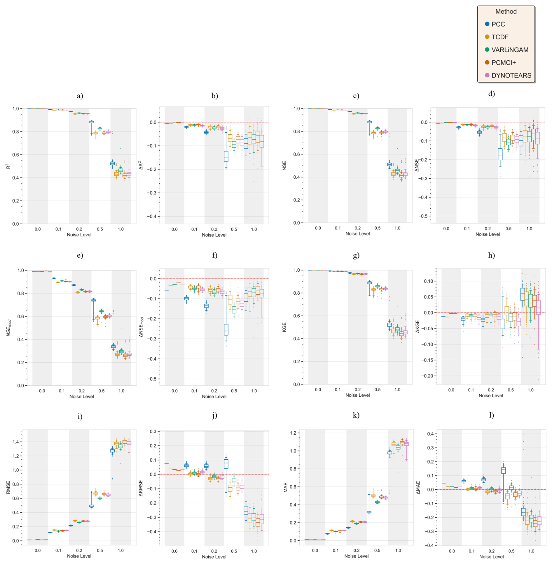
Figure C1Performance and error metrics for surface soil moisture predictions over a grid in Ganga basin. Similar to Fig. 7a–c and b–d, the figures show the performance (and error metrics) during the training period and the difference in performance during the testing and training periods. Further, figures show the results across different levels of noise in the system. The machine learning model used for prediction is support vector regression model.
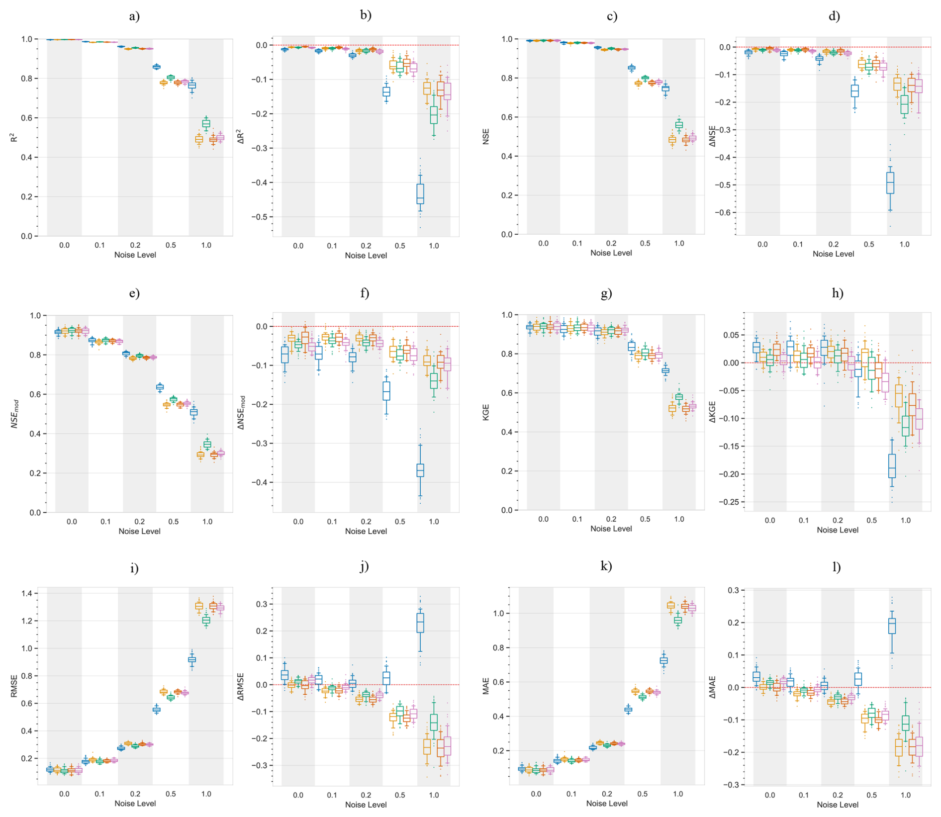
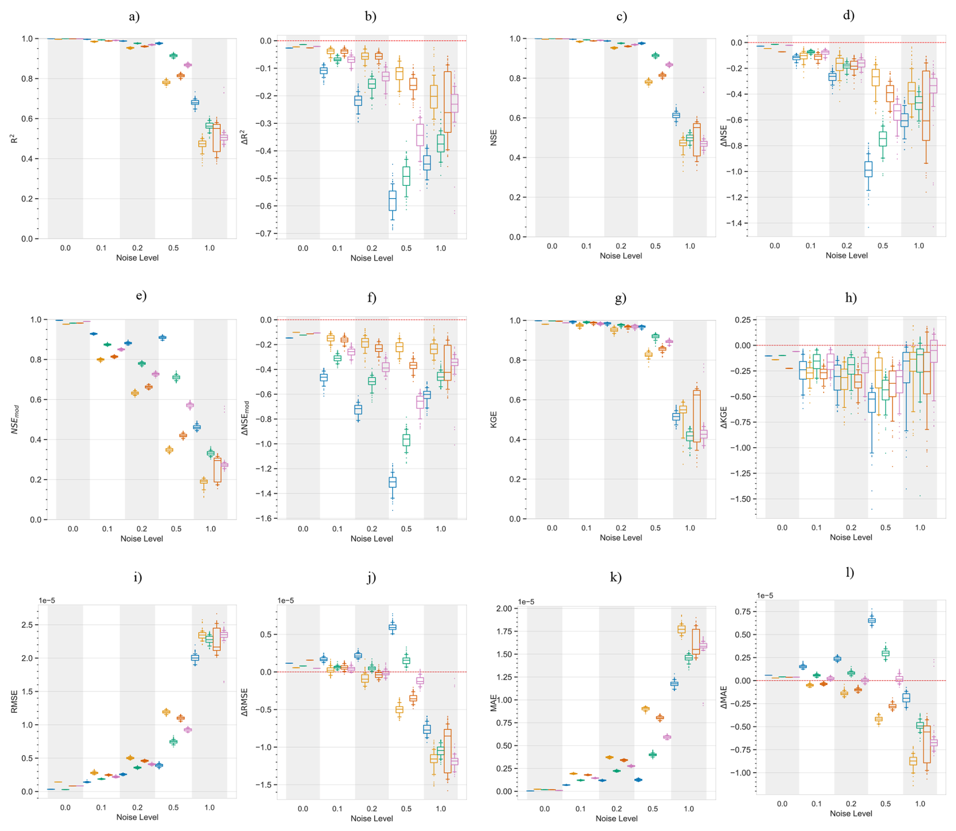
Figure C3Similar to Fig. C1 but scores for prediction of surface storm runoff in the Ganga basin. Training period: 1 January 2000 to 31 December 2003, Testing period: 1 January 2004 to 31 December 2005.
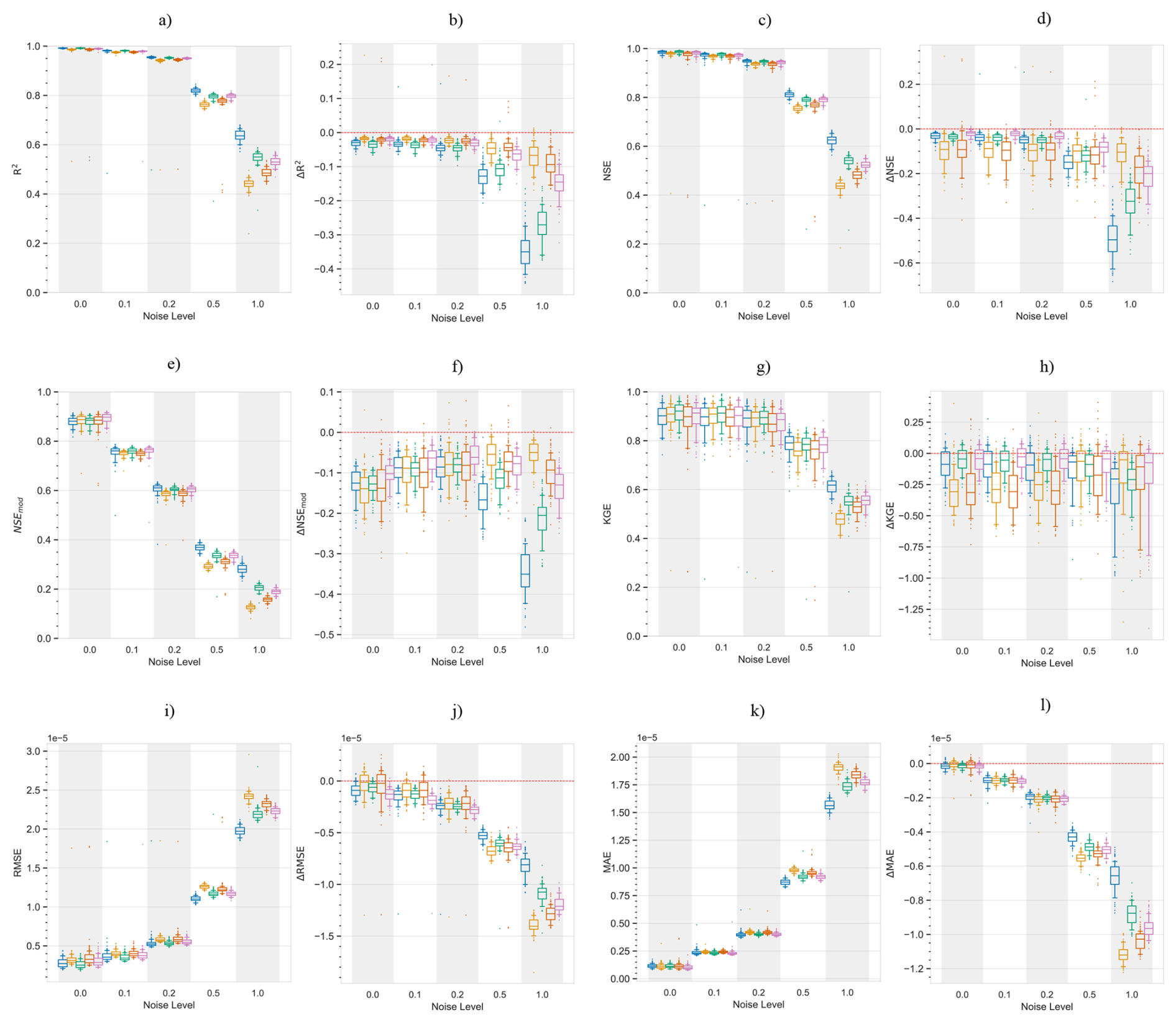
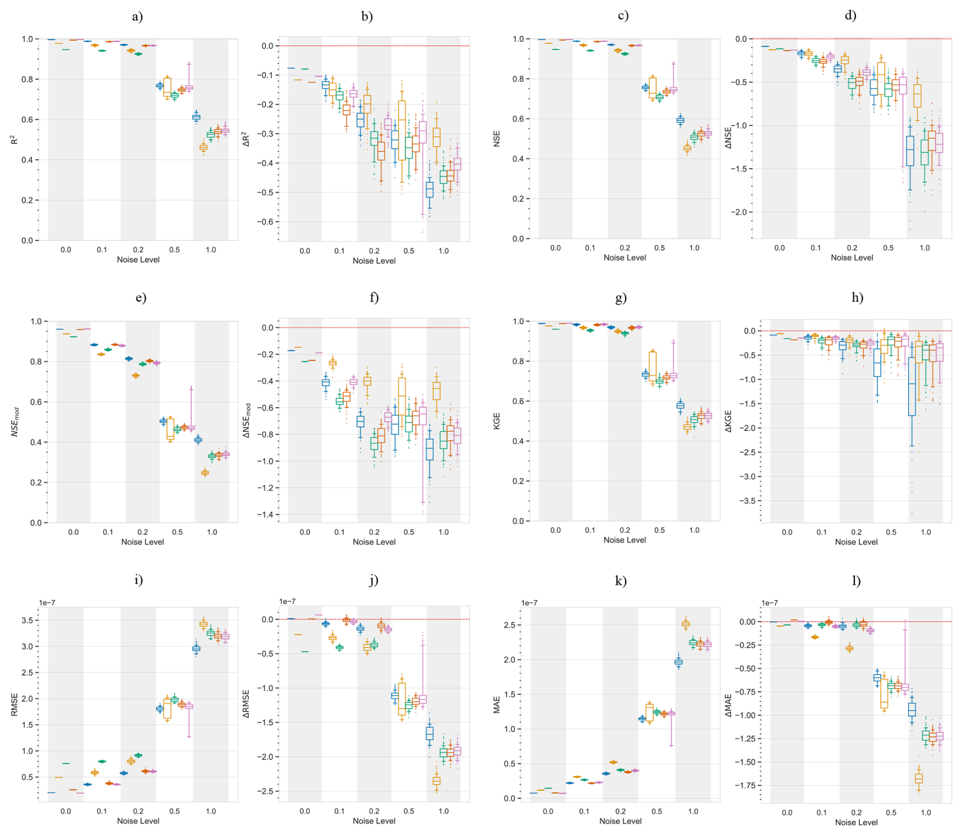
Figure C5Similar to Fig. C1 but scores for prediction of transpiration in the Murray basin. Training period: 1 January 2007 to 31 December 2012, Testing period: 1 January 2005 to 31 December 2006.
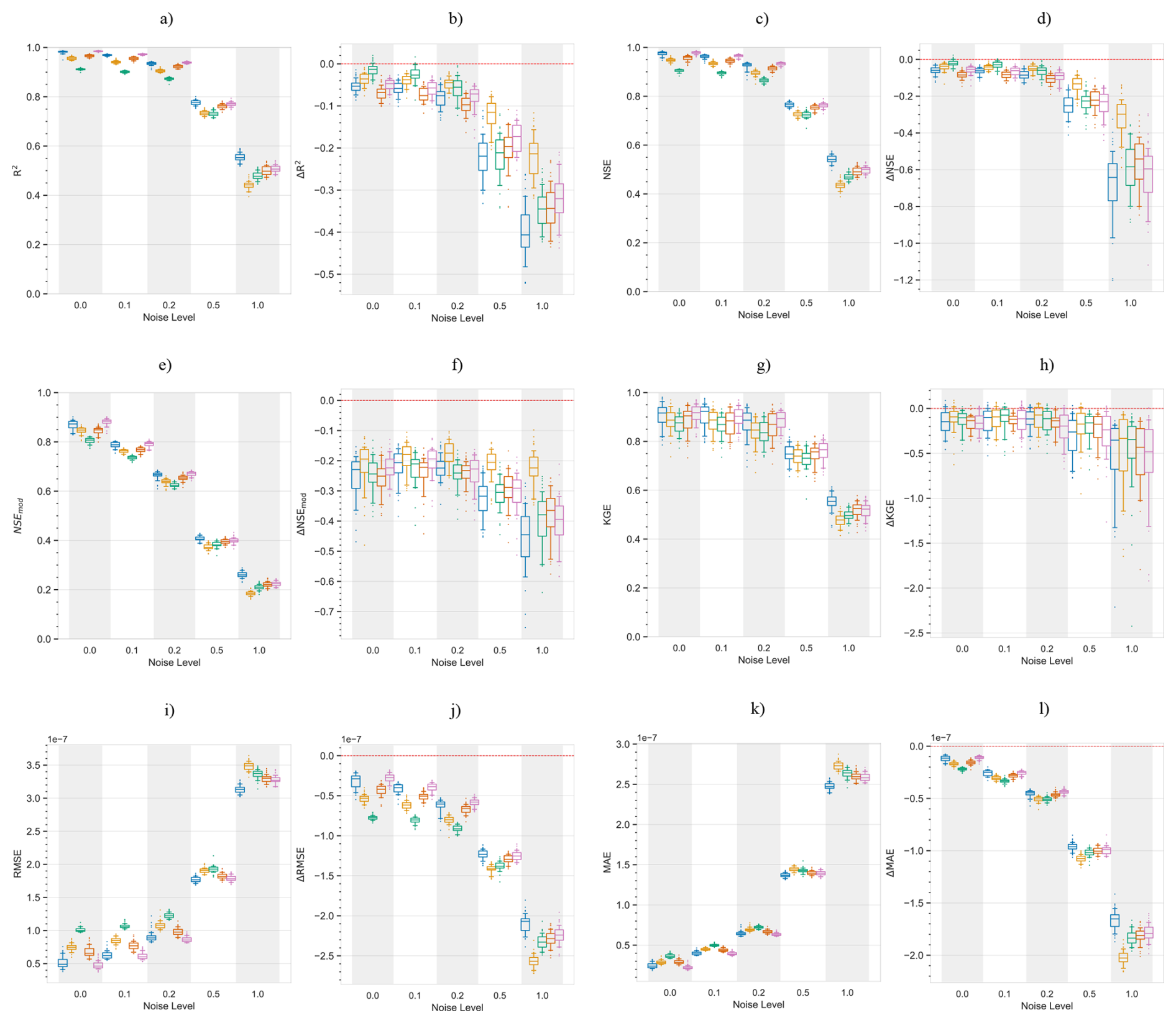
We tested the performance of various PCC and CD-based models under increasing training sample size. The details of the analysis and the results are presented below. This analysis is similar to the one shown in Sect. 2.7 with two key differences. First, we did not add any synthetically generated random noise to the data. Second, we trained separate models on increasing sample sizes of 75 d, 150 d, 6 months, 9 months, 1 year and 4 years. Then we evaluated their performance over the period of 1 January 2004 to 31 December 2004. The Table D1 summarises the analysis, while results are presented in Figs. D1, D2 and D3.
Table D1Experiment details for increasing sample size analysis.
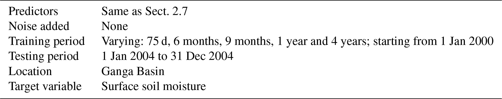
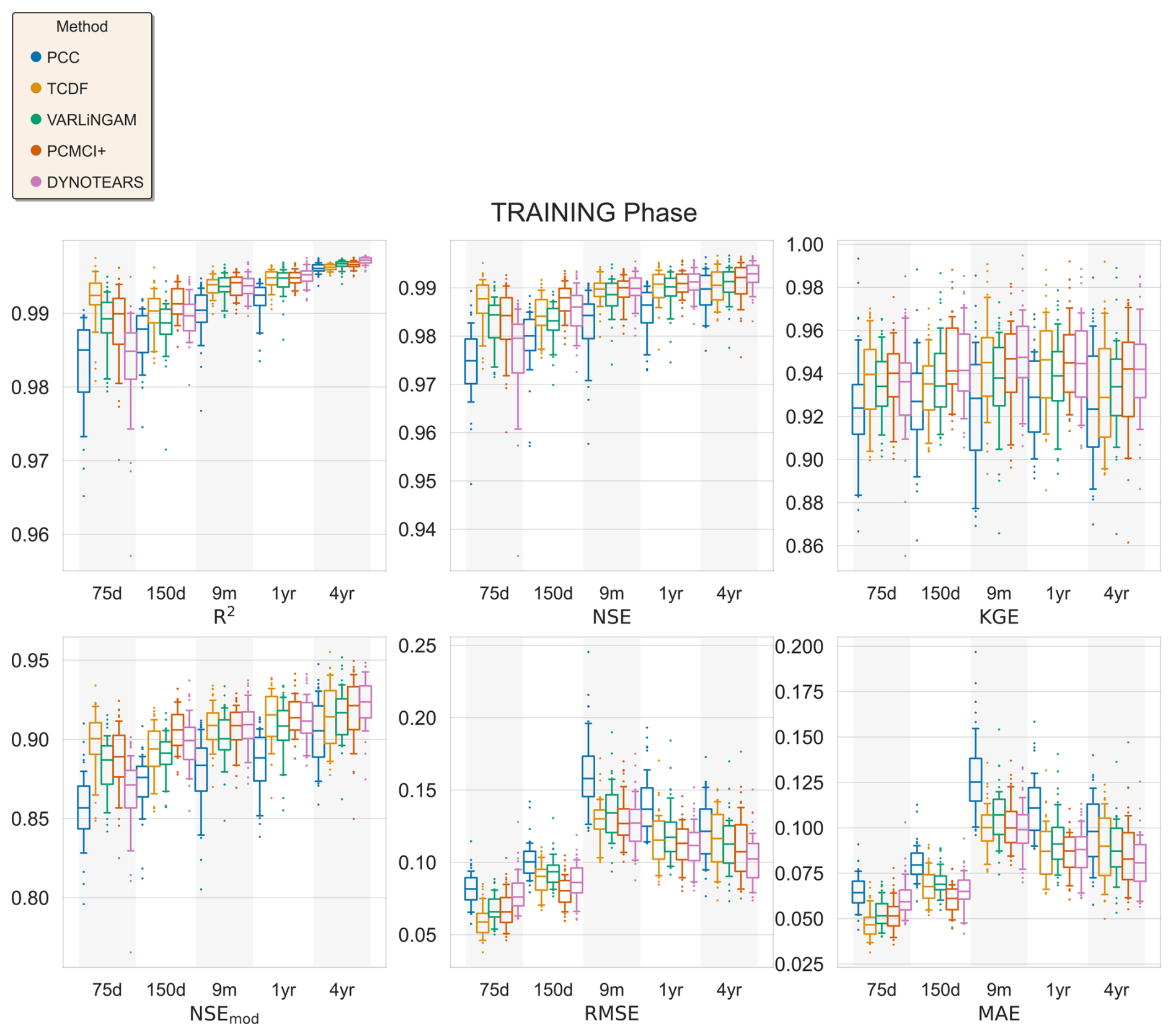
Figure D1Training period performance (and error) metrics of analysis with different training sample sizes (Appendix D). Results shown for increasing periods of training length.
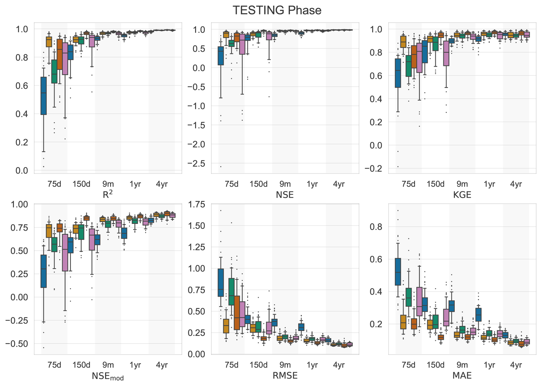
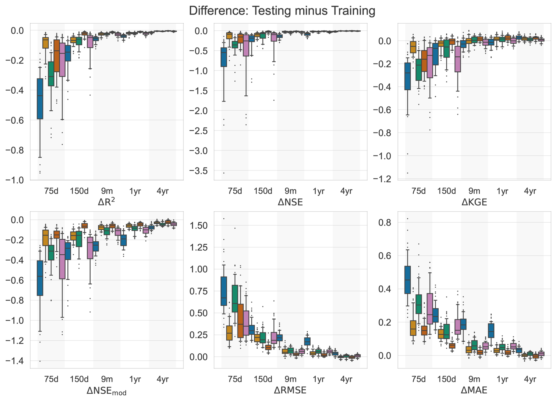
Since different methods, PCC and CD, return different numbers of predictors of the target variable, surface soil moisture, the analysis based on ML models and synthetically generated randomly gaussian noise can be affected by the dimensionality of the predictor set. Thus, in this analysis we select a common number of predictors for all methods. Towards this, we selected the predictors identified in Sect. 2.7 and filtered according to the criteria below. We call this approach TOP-K.
Table E1Selection criteria to implement the TOP-K approach for various methods.
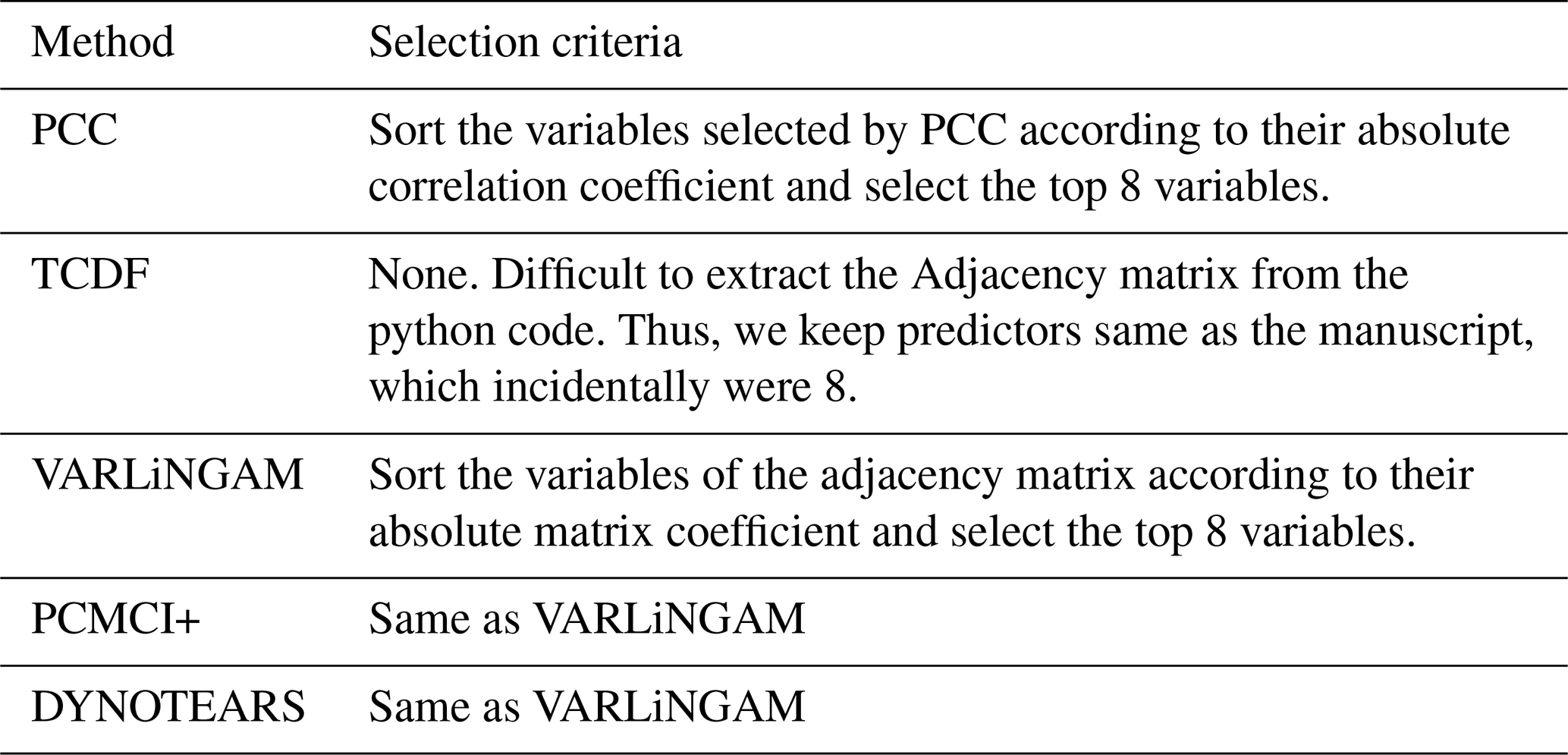
Table E2The set of predictors for each method, after filtering the respective set identified by each method respectively.
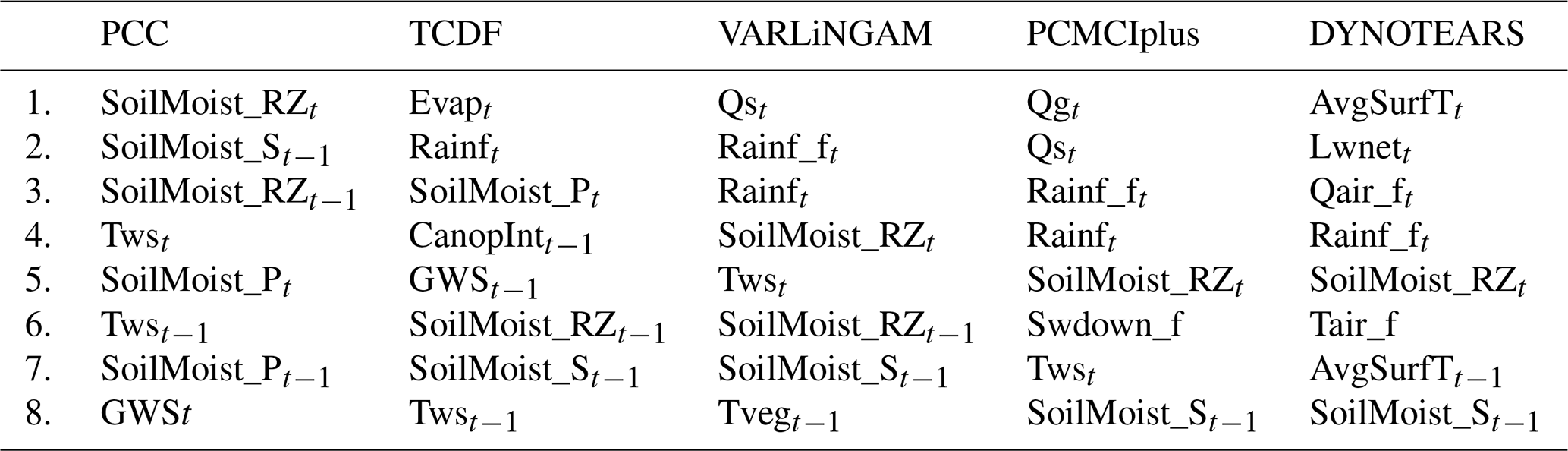
Table E3Details of analysis for ML models with the same dimensionality.
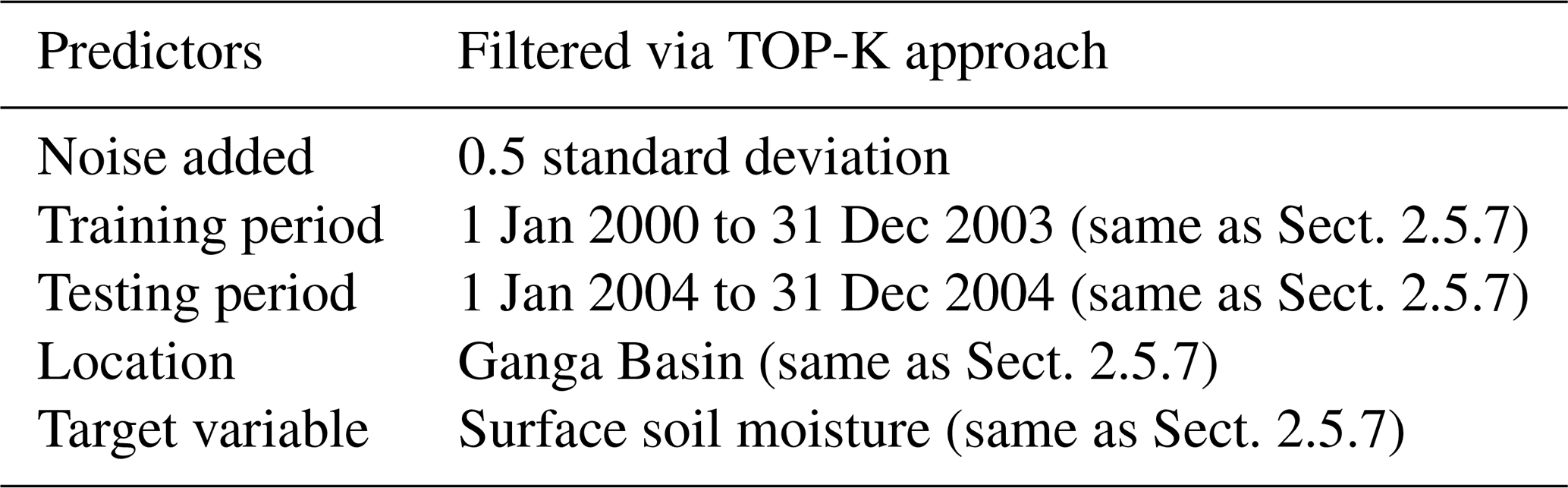
TOP-K approach. To select a common number of drivers for all methods we took the predictors selected by different methods (i.e. from Sect. 2.7) and filtered them with the approach in Table E1. We choose K=8, as it is equal to the actual number of true causal drivers of surface soil moisture. This yielded the equal number of predictors for each method (Table E2).
Details of machine learning models. Based on the set of predictors in Table E2, the machine learning models (feedforward neural network) were trained for surface soil moisture prediction. The model architecture was ensured to be the same for all the methods. The other details, i.e. the train and test period, location, target variable and noise level are the same as the Sect. 2.7. and listed in Table E3. The results of this analysis are presented in Figs. E1 and E2.
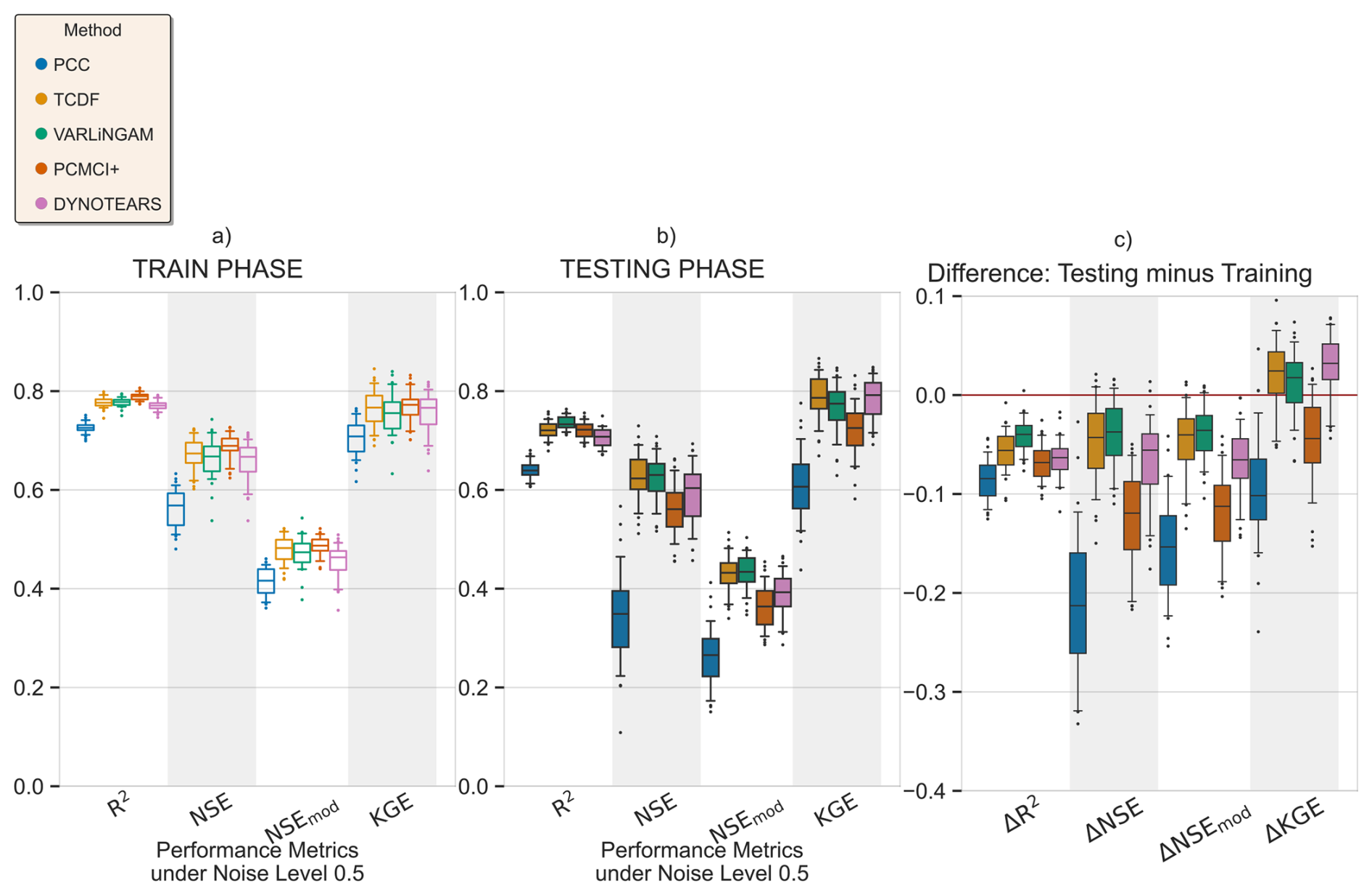
Figure E1Performance metrics for machine learning models based on predictors in Table E2. (a)–(c) for the training, testing and difference phases.
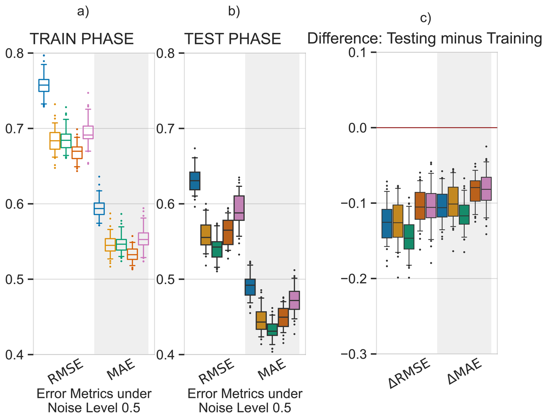
All the data used in the analysis was downloaded from NASA Earth Data and can be publicly accessed at https://doi.org/10.5067/LYHA9088MFWQ (last access: May 2024) (Li et al., 2018). All the analysis and plots created were done using publicly available python libraries. The analysis was done using standard python libraries like numpy (Harris et al., 2020), scipy (Virtanen et al., 2020), jupyter notebooks (Project Jupyter et al., 2018) and plots were created using matplotlib (Hunter, 2007) and seaborn (Waskom, 2021). The code for the CD algorithms are publicly available. For TCDF, the code is available on GitHub TCDF https://github.com/M-Nauta/TCDF (last access: May 2024). For VARLiNGAM the lingam python package was used: https://github.com/cdt15/lingam, (Ikeuchi et al., 2023). For PCMCI+ the tigramite python package was used: https://github.com/jakobrunge/tigramite (last access: May 2024). For DYNOTEARS the causalnex python package was used: https://causalnex.readthedocs.io/en/latest/ (last access: May 2024). The code to do the analysis and recreate the plots in this study are in https://github.com/lsmvivek/project_ci_eval (last access: May 2025) and https://doi.org/10.5281/zenodo.20337850 (Vivek Kumar, 2026).
VKY: Conceptualization, Data curation, Formal analysis, Methodology, Visualisation, Writing (original draft preparation), Writing (review and editing), MP: Supervision, Writing (review and editing), KF: Supervision, Writing (review and editing), DR: Supervision, Writing (review and editing), BDV: Conceptualization, Supervision, Writing (review and editing).
At least one of the (co-)authors is a member of the editorial board of Hydrology and Earth System Sciences. The peer-review process was guided by an independent editor, and the authors also have no other competing interests to declare.
Publisher's note: Copernicus Publications remains neutral with regard to jurisdictional claims made in the text, published maps, institutional affiliations, or any other geographical representation in this paper. The authors bear the ultimate responsibility for providing appropriate place names. Views expressed in the text are those of the authors and do not necessarily reflect the views of the publisher.
We thank the Editor, Yonggen Zhang for their valuable comments, which helped improve the discussion our results. Further, authors gratefully acknowledge the reviewers Uwe Ehret and Lu Li for their valuable comments, which improved the manuscript structure, strengthened the interpretation of the results and improved the analysis of causality-based time-series prediction models.
VKY gratefully acknowledges the financial support of Ministry of Education, Government of India through the PhD fellowship. Additional support was provided by the Melbourne India Postgraduate Academy (MIPA) fellowship.
This paper was edited by Yonggen Zhang and reviewed by Uwe Ehret and Lu Li.
Abbasizadeh, H., Maca, P., Hanel, M., Troldborg, M., and AghaKouchak, A.: Can causal discovery lead to a more robust prediction model for runoff signatures?, Hydrol. Earth Syst. Sci., 29, 4761–4790, https://doi.org/10.5194/hess-29-4761-2025, 2025. a
Ali, S., Hasan, U., Li, X., Faruque, O., Sampath, A., Huang, Y., Gani, M. O., and Wang, J.: Causality for Earth Science – A Review on Time-series and Spatiotemporal Causality Methods, arXiv [preprint], https://doi.org/10.48550/arXiv.2404.05746, 2024. a
Assaad, C. K., Devijver, E., and Gaussier, E.: Survey and Evaluation of Causal Discovery Methods for Time Series, J. Artif. Int. Res., 73, https://doi.org/10.1613/jair.1.13428, 2022. a, b, c, d, e, f
Barriopedro, D., García-Herrera, R., Ordóñez, C., Miralles, D. G., and Salcedo-Sanz, S.: Heat Waves: Physical Understanding and Scientific Challenges, Rev. Geophys., 61, e2022RG000780, https://doi.org/10.1029/2022RG000780, 2023. a
Beven, K.: Changing ideas in hydrology – The case of physically-based models, J. Hydrol., 105, 157–172, https://doi.org/10.1016/0022-1694(89)90101-7, 1989. a
Beven, K., Kirkby, M., Schofield, N., and Tagg, A.: Testing a physically-based flood forecasting model (TOPMODEL) for three U.K. catchments, J. Hydrol., 69, 119–143, https://doi.org/10.1016/0022-1694(84)90159-8, 1984. a
Beven, K. J. and Kirkby, M. J.: A physically based, variable contributing area model of basin hydrology/Un modèle à base physique de zone d'appel variable de l'hydrologie du bassin versant, Hydrol. Sci. J., 24, 43–69, https://doi.org/10.1080/02626667909491834, 1979. a, b, c, d
Bonotto, G., Peterson, T. J., Fowler, K., and Western, A. W.: Identifying Causal Interactions Between Groundwater and Streamflow Using Convergent Cross-Mapping, Water Resour. Res., 58, e2021WR030231, https://doi.org/10.1029/2021WR030231, 2022. a
Bui, H. X., Li, Y.-X., Sherwood, S. C., Reid, K. J., and Dommenget, D.: Assessing the soil moisture-precipitation feedback in Australia: CYGNSS observations, Environ. Res. Lett., 19, 014055, https://doi.org/10.1088/1748-9326/ad15b7, 2023. a
Byrd, R. H., Lu, P., Nocedal, J., and Zhu, C.: A Limited Memory Algorithm for Bound Constrained Optimization, SIAM Journal on Scientific Computing, 16, 1190–1208, https://doi.org/10.1137/0916069, 1995. a
Chauhan, T., Devanand, A., Roxy, M. K., Ashok, K., and Ghosh, S.: River interlinking alters land-atmosphere feedback and changes the Indian summer monsoon, Nat. Commun., 14, 5928, https://doi.org/10.1038/s41467-023-41668-x, 2023. a, b
Chicco, D. and Jurman, G.: The advantages of the Matthews correlation coefficient (MCC) over F1 score and accuracy in binary classification evaluation, BMC Genomics, 21, 6, https://doi.org/10.1186/s12864-019-6413-7, 2020. a
Chollet, F.: Keras, https://keras.io (last access: May 2024), 2015. a
Christian, J. I., Hobbins, M., Hoell, A., Otkin, J. A., Ford, T. W., Cravens, A. E., Powlen, K. A., Wang, H., and Mishra, V.: Flash drought: A state of the science review, WIREs Water, 11, e1714, https://doi.org/10.1002/wat2.1714, 2024. a
Clapp, R. B. and Hornberger, G. M.: Empirical equations for some soil hydraulic properties, Water Resour. Res., 14, 601–604, https://doi.org/10.1029/WR014i004p00601, 1978. a, b, c
Cunningham, W. J. C. W. H. and Schrijver, W. R. P. A.: Combinatorial optimization, NY, United States, https://doi.org/10.1002/9781118033142, 1998. a
Delforge, D., de Viron, O., Vanclooster, M., Van Camp, M., and Watlet, A.: Detecting hydrological connectivity using causal inference from time series: synthetic and real karstic case studies, Hydrol. Earth Syst. Sci., 26, 2181–2199, https://doi.org/10.5194/hess-26-2181-2022, 2022. a, b, c, d, e, f
Devanand, A., Roxy, M. K., and Ghosh, S.: Coupled Land-Atmosphere Regional Model Reduces Dry Bias in Indian Summer Monsoon Rainfall Simulated by CFSv2, Geophys. Res. Lett., 45, 2476–2486, https://doi.org/10.1002/2018GL077218, 2018. a
Ducharne, A., Koster, R. D., Suarez, M. J., Stieglitz, M., and Kumar, P.: A catchment-based approach to modeling land surface processes in a general circulation model: 2. Parameter estimation and model demonstration, J. Geophys. Res.-Atmos., 105, 24823–24838, https://doi.org/10.1029/2000JD900327, 2000. a, b
Dutra, E., Balsamo, G., Calvet, J., Munier, S., Burke, S., Fink, G., van Dijk, A., Martinez-de la Torre, A., van Beek, R., De Roo, A., Balsamo, G., Calvet, J.-C., Munier, S., Burke, S., Fink, G., van Dijk, A., Martinez-de la Torre, A., van Beek, R., De Roo, A., and Polcher, J.: Report on the improved water resources reanalysis, Tech. rep., EartH2Observe, https://doi.org/10.13140/RG.2.2.14523.67369, 2017. a
Feng, D., Beck, H., Lawson, K., and Shen, C.: The suitability of differentiable, physics-informed machine learning hydrologic models for ungauged regions and climate change impact assessment, Hydrol. Earth Syst. Sci., 27, 2357–2373, https://doi.org/10.5194/hess-27-2357-2023, 2023. a
Gong, C., Zhang, C., Yao, D., Bi, J., Li, W., and Xu, Y.: Causal Discovery from Temporal Data: An Overview and New Perspectives, ACM Comput. Surv., 57, https://doi.org/10.1145/3705297, 2024. a, b
Gong, M., Zhang, K., Schölkopf, B., Glymour, C., and Tao, D.: Causal discovery from temporally aggregated time series, in: Proceedings of the 33rd Conference on Uncertainty in Artificial Intelligence ID 269, edited by: Elidan, G., Kersting, K., and Ihler, A. T., AUAI Press, Corvallis, Oregon, USA, 2017. a
Goodwell, A. E., Jiang, P., Ruddell, B. L., and Kumar, P.: Debates – Does Information Theory Provide a New Paradigm for Earth Science? Causality, Interaction, and Feedback, Water Resour. Res., 56, e2019WR024940, https://doi.org/10.1029/2019WR024940, 2020. a
Gosling, S. N., Müller Schmied, H., Betts, R., Chang, J., Chen, H., Ciais, P., Dankers, R., Döll, P., Eisner, S., Flörke, M., Gerten, D., Grillakis, M., Hagemann, S., Hanasaki, N., Huang, M., Huang, Z., Jerez, S., Kim, H., Koutroulis, A., Leng, G., Liu, J., Liu, X., Mao, G., Masaki, Y., Montavez, J. P., Morfopoulos, C., Oki, T., Orth, R., Ostberg, S., Papadimitriou, L., Pokhrel, Y., Portmann, F., Qi, W., Satoh, Y., Seneviratne, S., Sommer, P. S., Stacke, T., Tang, Q., Tsanis, I., Wada, Y., Wang, X., Zhou, T., Büchner, M., Schewe, J., and Zhao, F.: ISIMIP2a Simulation Data from the Global Water Sector, ISIMIP2a Simulation Data from the Global Water Sector, ISIMIP Repository [data set], https://doi.org/10.48364/ISIMIP.882536, 2023. a, b
Granger, C. W. J.: Investigating Causal Relations by Econometric Models and Cross-spectral Methods, Econometrica, 37, 424–438, https://doi.org/10.2307/1912791, 1969. a, b
Guillod, B. P., Orlowsky, B., Miralles, D. G., Teuling, A. J., and Seneviratne, S. I.: Reconciling spatial and temporal soil moisture effects on afternoon rainfall, Nat. Commun., 6, 6443, https://doi.org/10.1038/ncomms7443, 2015. a
Harris, C. R., Millman, K. J., van der Walt, S. J., Gommers, R., Virtanen, P., Cournapeau, D., Wieser, E., Taylor, J., Berg, S., Smith, N. J., Kern, R., Picus, M., Hoyer, S., van Kerkwijk, M. H., Brett, M., Haldane, A., del Río, J. F., Wiebe, M., Peterson, P., Gérard-Marchant, P., Sheppard, K., Reddy, T., Weckesser, W., Abbasi, H., Gohlke, C., and Oliphant, T. E.: Array programming with NumPy, Nature, 585, 357–362, https://doi.org/10.1038/s41586-020-2649-2, 2020. a
Hasan, U., Hossain, E., and Gani, M. O.: A Survey on Causal Discovery Methods for I.I.D. and Time Series Data, arXiv [preprint], https://doi.org/10.48550/arXiv.2303.15027, 2024. a
Höge, M., Scheidegger, A., Baity-Jesi, M., Albert, C., and Fenicia, F.: Improving hydrologic models for predictions and process understanding using neural ODEs, Hydrol. Earth Syst. Sci., 26, 5085–5102, https://doi.org/10.5194/hess-26-5085-2022, 2022. a
Holder, R.: Multiple regression in hydrology, Institute of hydrology, ISBN 0948540001, 1985. a
Hunter, J. D.: Matplotlib: A 2D graphics environment, Comput. Sci. Eng., 9, 90–95, https://doi.org/10.1109/MCSE.2007.55, 2007. a
Hyvärinen, A., Karhunen, J., and Oja, E.: What is Independent Component Analysis?, chap. 7, 145–164, John Wiley and Sons, Ltd, ISBN 9780471221319, https://doi.org/10.1002/0471221317.ch7, 2001. a, b
Hyvärinen, A., Shimizu, S., and Hoyer, P. O.: Causal modelling combining instantaneous and lagged effects: an identifiable model based on non-Gaussianity, in: Proceedings of the 25th International Conference on Machine Learning, ICML '08, p. 424–431, Association for Computing Machinery, New York, NY, USA, ISBN 9781605582054, https://doi.org/10.1145/1390156.1390210, 2008. a, b, c
Ikeuchi, T., Ide, M., Zeng, Y., Maeda, T. N., and Shimizu, S.: Python package for causal discovery based on LiNGAM, J. Mach. Learn. Res., 24, 1–8, 2023 (code available at: https://github.com/cdt15/lingam, last access: May 2024). a
Jackson, E. K., Roberts, W., Nelsen, B., Williams, G. P., Nelson, E. J., and Ames, D. P.: Introductory overview: Error metrics for hydrologic modelling – A review of common practices and an open source library to facilitate use and adoption, Environ. Model. Softw., 119, 32–48, https://doi.org/10.1016/j.envsoft.2019.05.001, 2019. a
Kirchner, J. W.: Getting the right answers for the right reasons: Linking measurements, analyses, and models to advance the science of hydrology, Water Resour. Res., 42, https://doi.org/10.1029/2005WR004362, 2006. a
Koster, R. D. and Suarez, M. J.: Modeling the land surface boundary in climate models as a composite of independent vegetation stands, J. Geophys. Res.-Atmos., 97, 2697–2715, https://doi.org/10.1029/91JD01696, 1992. a, b, c
Koster, R. D. and Suarez, M. J.: Energy and water balance calculations in the Mosaic LSM, NASA Technical Memorandum 104606, Technical Report Series on Global Modeling and Data Assimilation, vol. 9, 60 pp., 1996. a
Koster, R. D., Suarez, M. J., Ducharne, A., Stieglitz, M., and Kumar, P.: A catchment-based approach to modeling land surface processes in a general circulation model: 1. Model structure, J. Geophys. Res.-Atmos., 105, 24809–24822, https://doi.org/10.1029/2000JD900327, 2000. a, b, c
Kratzert, F., Klotz, D., Herrnegger, M., Sampson, A. K., Hochreiter, S., and Nearing, G. S.: Toward Improved Predictions in Ungauged Basins: Exploiting the Power of Machine Learning, Water Resour. Res., 55, 11344–11354, https://doi.org/10.1029/2019WR026065, 2019. a, b, c
Lehner, B., Verdin, K., and Jarvis, A.: New Global Hydrography Derived From Spaceborne Elevation Data, Eos, Transactions American Geophysical Union, 89, 93–94, https://doi.org/10.1029/2008EO100001, 2008. a
Li, B., Beaudoing, H., and Rodell, M.: NASA/GSFC/HSL (2018), GLDAS Catchment Land Surface Model L4 daily 0.25 x 0.25 degree V2.0, Greenbelt, Maryland, USA, Goddard Earth Sciences Data and Information Services Center (GES DISC), Tech. rep., Goddard Earth Sciences Data and Information Services Center (GES DISC) [data set], https://doi.org/10.5067/LYHA9088MFWQ (last access: 17 April 2024), 2018. a, b, c, d
Li, L., Dai, Y., Shangguan, W., Wei, Z., Wei, N., and Li, Q.: Causality-Structured Deep Learning for Soil Moisture Predictions, J. Hydrometeorol., 23, 1315–1331, https://doi.org/10.1175/JHM-D-21-0206.1, 2022. a
Lynch-Stieglitz, M.: The development and validation of a simple snow model for the GISS GCM, J. Climate, 7, 1842–1855, https://doi.org/10.1175/1520-0442(1994)007<1842:TDAVOA>2.0.CO;2, 1994. a, b
Mishra, A., Mukherjee, S., Merz, B., Singh, V. P., Wright, D. B., Villarini, G., Paul, S., Kumar, D. N., Khedun, C. P., Niyogi, D., Schumann, G., and Stedinger, J. R.: An Overview of Flood Concepts, Challenges, and Future Directions, J. Hydrol. Eng., 27, 03122001, https://doi.org/10.1061/(ASCE)HE.1943-5584.0002164, 2022. a
Nauta, M., Bucur, D., and Seifert, C.: Causal Discovery with Attention-Based Convolutional Neural Networks, Machine Learning and Knowledge Extraction, 1, 312–340, https://doi.org/10.3390/make1010019, 2019. a, b, c, d, e, f
Nearing, G. S., Kratzert, F., Sampson, A. K., Pelissier, C. S., Klotz, D., Frame, J. M., Prieto, C., and Gupta, H. V.: What Role Does Hydrological Science Play in the Age of Machine Learning?, Water Resour. Res., 57, e2020WR028091, https://doi.org/10.1029/2020WR028091, 2021. a, b, c
Ombadi, M., Nguyen, P., Sorooshian, S., and Hsu, K.-l.: Evaluation of Methods for Causal Discovery in Hydrometeorological Systems, Water Resour. Res., 56, e2020WR027251, https://doi.org/10.1029/2020WR027251, 2020. a, b, c, d, e, f, g, h, i, j, k, l, m, n, o, p, q, r
Pamfil, R., Sriwattanaworachai, N., Desai, S., Pilgerstorfer, P., Georgatzis, K., Beaumont, P., and Aragam, B.: DYNOTEARS: Structure Learning from Time-Series Data, Proceedings of Machine Learning Research, arXiv, 108, 1595–1605, https://doi.org/10.48550/arXiv.2002.00498, 2020. a, b, c
Park, Y. W. and Klabjan, D.: Bayesian Network Learning via Topological Order, J. Mach. Learn. Res., 18, 1–32, 2017. a
Pearl, J.: Graphs, Causality, and Structural Equation Models, Sociol. Method. Res., 27, 226–284, https://doi.org/10.1177/0049124198027002004, 1998. a
Pearl, J.: Causality, Cambridge University Press, ISBN 978-0-521-89560-6, 2009. a, b, c
Pedregosa, F., Varoquaux, G., Gramfort, A., Michel, V., Thirion, B., Grisel, O., Blondel, M., Prettenhofer, P., Weiss, R., Dubourg, V., Vanderplas, J., Passos, A., Cournapeau, D., Brucher, M., Perrot, M., and Duchesnay, E.: Scikit-learn: Machine Learning in Python, J. Mach. Learn. Res., 12, 2825–2830, 2011. a
Peel, M. C. and McMahon, T. A.: Historical development of rainfall-runoff modeling, WIREs Water, 7, e1471, https://doi.org/10.1002/wat2.1471, 2020. a
Peters, J., Janzing, D., and Schölkopf, B.: Elements of causal inference: foundations and learning algorithms, The MIT Press, ISBN 9780262037310, 2017. a, b, c
Powers, D. M. W.: Evaluation: from precision, recall and F-measure to ROC, informedness, markedness and correlation, arXiv [preprint], https://doi.org/10.48550/arXiv.2010.16061, 2020. a, b
Project Jupyter, Bussonnier, M., Forde, J., Freeman, J., Granger, B., Head, T., Holdgraf, C., Kelley, K., Nalvarte, G., Osheroff, A., Pacer, M., Panda, Y., Perez, F., Kelley, B. R., and Willing, C.: Binder 2.0 – Reproducible, interactive, sharable environments for science at scale, in: Proceedings of the 17th Python in Science Conference, edited by: Akici, F., Lippa, D., Niederhut, D., and Pacer, M., 113–120, https://doi.org/10.25080/Majora-4af1f417-011, 2018. a
Rinderer, M., Ali, G., and Larsen, L. G.: Assessing structural, functional and effective hydrologic connectivity with brain neuroscience methods: State-of-the-art and research directions, Earth-Sci. Rev., 178, 29–47, https://doi.org/10.1016/j.earscirev.2018.01.009, 2018. a
Ruddell, B. L. and Kumar, P.: Ecohydrologic process networks: 1. Identification, Water Resour. Res., 45, https://doi.org/10.1029/2008WR007279, 2009. a
Runge, J.: Causal network reconstruction from time series: From theoretical assumptions to practical estimation, Chaos, 28, 075310, https://doi.org/10.1063/1.5025050, 2018. a, b
Runge, J.: Discovering contemporaneous and lagged causal relations in autocorrelated nonlinear time series datasets, arXiv [preprint], https://doi.org/10.48550/arXiv.2003.03685, 2022. a, b, c, d, e, f, g, h
Runge, J., Heitzig, J., Petoukhov, V., and Kurths, J.: Escaping the Curse of Dimensionality in Estimating Multivariate Transfer Entropy, Phys. Rev. Lett., 108, 258701, https://doi.org/10.1103/PhysRevLett.108.258701, 2012. a, b
Runge, J., Nowack, P., Kretschmer, M., Flaxman, S., and Sejdinovic, D.: Detecting and quantifying causal associations in large nonlinear time series datasets, Sci. Adv., 5, eaau4996, https://doi.org/10.1126/sciadv.aau4996, 2019a. a, b
Runge, J., Nowack, P., Kretschmer, M., Flaxman, S., and Sejdinovic, D.: Detecting and quantifying causal associations in large nonlinear time series datasets, Sci. Adv., 5, eaau4996, https://doi.org/10.1126/sciadv.aau4996, 2019b. a, b, c
Samek, W., Montavon, G., Vedaldi, A., Hansen, L. K., and Müller, K.-R.: Explainable AI: interpreting, explaining and visualizing deep learning, vol. 11700, Springer Nature, https://doi.org/10.1007/978-3-030-28954-6, 2019. a
Schellekens, J., Dutra, E., Martínez-de la Torre, A., Balsamo, G., van Dijk, A., Sperna Weiland, F., Minvielle, M., Calvet, J.-C., Decharme, B., Eisner, S., Fink, G., Flörke, M., Peßenteiner, S., van Beek, R., Polcher, J., Beck, H., Orth, R., Calton, B., Burke, S., Dorigo, W., and Weedon, G. P.: A global water resources ensemble of hydrological models: the eartH2Observe Tier-1 dataset, Earth Syst. Sci. Data, 9, 389–413, https://doi.org/10.5194/essd-9-389-2017, 2017. a, b
Schreiber, T.: Measuring Information Transfer, Phys. Rev. Lett., 85, 461–464, https://doi.org/10.1103/PhysRevLett.85.461, 2000. a
Seneviratne, S. I., Corti, T., Davin, E. L., Hirschi, M., Jaeger, E. B., Lehner, I., Orlowsky, B., and Teuling, A. J.: Investigating soil moisture–climate interactions in a changing climate: A review, Earth-Sci. Rev., 99, 125–161, https://doi.org/10.1016/j.earscirev.2010.02.004, 2010. a
Shannon, C. E.: A Mathematical Theory of Communication, Bell System Technical Journal, 27, 379–423, https://doi.org/10.1002/j.1538-7305.1948.tb01338.x, 1948. a
Sheffield, J., Goteti, G., and Wood, E. F.: Development of a 50-Year High-Resolution Global Dataset of Meteorological Forcings for Land Surface Modeling, J. Climate, 19, 3088–3111, https://doi.org/10.1175/JCLI3790.1, 2006. a
Shi, H., Zhao, Y., Liu, S., Cai, H., and Zhou, Z.: A New Perspective on Drought Propagation: Causality, Geophys. Res. Lett., 49, e2021GL096758, https://doi.org/10.1029/2021GL096758, 2022. a
Shimizu, S., Hoyer, P., Hyvärinen, A., and Kerminen, A.: A linear non-gaussian acyclic model for causal discovery, J. Mach. Learn. Res., 7, 2003–2030, 2006. a
Spirtes, P. and Glymour, C.: An algorithm for fast recovery of sparse causal graphs, Soc. Sci. Comput. Rev., 9, 62–72, https://doi.org/10.1177/089443939100900106, 1991. a, b
Sugihara, G., May, R., Ye, H., hao Hsieh, C., Deyle, E., Fogarty, M., and Munch, S.: Detecting Causality in Complex Ecosystems, Science, 338, 496–500, https://doi.org/10.1126/science.1227079, 2012. a, b, c, d, e
Tasker, G. D.: Hydrologic regression with weighted least squares, Water Resour. Res., 16, 1107–1113, https://doi.org/10.1029/WR016i006p01107, 1980. a
Tripathy, K. P. and Mishra, A. K.: Deep learning in hydrology and water resources disciplines: concepts, methods, applications, and research directions, J. Hydrol., 628, 130458, https://doi.org/10.1016/j.jhydrol.2023.130458, 2024. a
Tuttle, S. E. and Salvucci, G. D.: Confounding factors in determining causal soil moisture-precipitation feedback, Water Resour. Res., 53, 5531–5544, https://doi.org/10.1002/2016WR019869, 2017. a, b, c
Van Oldenborgh, G. J., Wehner, M. F., Vautard, R., Otto, F. E. L., Seneviratne, S. I., Stott, P. A., Hegerl, G. C., Philip, S. Y., and Kew, S. F.: Attributing and Projecting Heatwaves Is Hard: We Can Do Better, Earth's Future, 10, e2021EF002271, https://doi.org/10.1029/2021EF002271, 2022. a
Vázquez-Patiño, A., Samaniego, E., Campozano, L., and Avilés, A.: Effectiveness of causality-based predictor selection for statistical downscaling: a case study of rainfall in an Ecuadorian Andes basin, Theor. Appl. Climatol., 150, 987–1013, https://doi.org/10.1007/s00704-022-04205-2, 2022. a
Virtanen, P., Gommers, R., Oliphant, T. E., Haberland, M., Reddy, T., Cournapeau, D., Burovski, E., Peterson, P., Weckesser, W., Bright, J., van der Walt, S. J., Brett, M., Wilson, J., Millman, K. J., Mayorov, N., Nelson, A. R. J., Jones, E., Kern, R., Larson, E., Carey, C. J., Polat, İ., Feng, Y., Moore, E. W., VanderPlas, J., Laxalde, D., Perktold, J., Cimrman, R., Henriksen, I., Quintero, E. A., Harris, C. R., Archibald, A. M., Ribeiro, A. H., Pedregosa, F., van Mulbregt, P., and SciPy 1.0 Contributors: SciPy 1.0: Fundamental Algorithms for Scientific Computing in Python, Nature Methods, 17, 261–272, https://doi.org/10.1038/s41592-019-0686-2, 2020. a
Vivek Kumar, Y.: lsmvivek/project_ci_eval: Release for Zenodo archive (hess-accepted-v1), Zenodo [code], https://doi.org/10.5281/zenodo.20337850, 2026. a
Voortman, M., Dash, D., and Druzdzel, M. J.: Learning why things change: the difference-based causality learner, in: Proceedings of the Twenty-Sixth Conference on Uncertainty in Artificial Intelligence, UAI'10, 641–650, AUAI Press, Arlington, Virginia, USA, ISBN 9780974903965, 2010. a
Wang, L., Gu, H., Liu, L., Liang, X., Chen, S., and Xu, Y.-P.: Revealing joint evolutions and causal interactions in complex ecohydrological systems by a network-based framework, Hydrol. Earth Syst. Sci., 29, 361–379, https://doi.org/10.5194/hess-29-361-2025, 2025. a
Wang, Y., Yang, J., Chen, Y., De Maeyer, P., Li, Z., and Duan, W.: Detecting the causal effect of soil moisture on precipitation using convergent cross mapping, Sci. Rep., 8, 12171, https://doi.org/10.1038/s41598-018-30669-2, 2018. a
Warszawski, L., Frieler, K., Huber, V., Piontek, F., Serdeczny, O., and Schewe, J.: The Inter-Sectoral Impact Model Intercomparison Project (ISI–MIP): Project framework, P. Natl. Acad. Sci. USA, 111, 3228–3232, https://doi.org/10.1073/pnas.1312330110, 2014. a
Waskom, M. L.: seaborn: statistical data visualization, J. Open Source Softw., 6, 3021, https://doi.org/10.21105/joss.03021, 2021. a
Wu, C. and Chau, K.: Rainfall–runoff modeling using artificial neural network coupled with singular spectrum analysis, J. Hydrol., 399, 394–409, https://doi.org/10.1016/j.jhydrol.2011.01.017, 2011. a
Wu, T., Xu, L., Lv, Y., Cai, R., Pan, Z., Zhang, X., Zhang, X., and Chen, N.: Integrating causal inference with ConvLSTM networks for spatiotemporal forecasting of root zone soil moisture, J. Hydrol., 659, 133246, https://doi.org/10.1016/j.jhydrol.2025.133246, 2025. a
Xu, T. and Liang, F.: Machine learning for hydrologic sciences: An introductory overview, WIREs Water, 8, e1533, https://doi.org/10.1002/wat2.1533, 2021. a
Yuan, K., Zhu, Q., Li, F., Riley, W. J., Torn, M., Chu, H., McNicol, G., Chen, M., Knox, S., Delwiche, K., Wu, H., Baldocchi, D., Ma, H., Desai, A. R., Chen, J., Sachs, T., Ueyama, M., Sonnentag, O., Helbig, M., Tuittila, E.-S., Jurasinski, G., Koebsch, F., Campbell, D., Schmid, H. P., Lohila, A., Goeckede, M., Nilsson, M. B., Friborg, T., Jansen, J., Zona, D., Euskirchen, E., Ward, E. J., Bohrer, G., Jin, Z., Liu, L., Iwata, H., Goodrich, J., and Jackson, R.: Causality guided machine learning model on wetland CH4 emissions across global wetlands, Agr. Forest Meteorol., 324, 109115, https://doi.org/10.1016/j.agrformet.2022.109115, 2022. a
Zhang, W. and Montgomery, D. R.: Digital elevation model grid size, landscape representation, and hydrologic simulations, Water Resour. Res., 30, 1019–1028, https://doi.org/10.1029/93WR03553, 1994. a
Zhang, Y., Chiew, F. H. S., Li, M., and Post, D.: Predicting Runoff Signatures Using Regression and Hydrological Modeling Approaches, Water Resour. Res., 54, 7859–7878, https://doi.org/10.1029/2018WR023325, 2018. a
Zheng, X., Aragam, B., Ravikumar, P. K., and Xing, E. P.: DAGs with NO TEARS: Continuous Optimization for Structure Learning, in: Advances in Neural Information Processing Systems, edited by Bengio, S., Wallach, H., Larochelle, H., Grauman, K., Cesa-Bianchi, N., and Garnett, R., vol. 31, Curran Associates, Inc., arXiv [preprint], https://doi.org/10.48550/arXiv.1803.01422, 2018. a
Zou, L., Zha, Y., Diao, Y., Tang, C., Gu, W., and Shao, D.: Coupling the causal inference and informer networks for short-term forecasting in irrigation water usage, Water Resour. Manage., 37, 427–449, https://doi.org/10.1007/s11269-022-03381-0, 2023. a, b
- Abstract
- Introduction
- Methodology and Methods
- Results
- Discussion
- Summary, Conclusions and Outlook
- Appendix A: CLSM model: Description, modelling schemes and generating equations
- Appendix B: Algorithm settings
- Appendix C: Machine learning model for time-series predictions
- Appendix D: PCC and CD-based ML models under increasing training sample size
- Appendix E: PCC and CD-based ML models under the same dimensionality
- Code and data availability
- Author contributions
- Competing interests
- Disclaimer
- Acknowledgements
- Financial support
- Review statement
- References