Can streamflow observations constrain snow mass reconstructions? Lessons from two synthetic numerical experiments

Historical estimates of seasonal snow mass are key to understanding snowmelt-driven streamflow and climate change impacts on mountain water resources. However, direct observations of snow mass are sparse in space and time, forcing most reconstructions to rely on snow models driven by uncertain meteorological inputs. While ground-based and satellite snow observations are commonly used to constrain these models, their potential is limited in data-scarce regions and before the onset of satellite monitoring. Here, we investigate the potential of streamflow observations as an additional source of information to improve historical snow mass reconstructions. We introduce an inverse hydrological modeling framework that selects realistic snow mass realizations based on the accuracy of their streamflow response. Before real-world application, we test the framework in two synthetic experiments. Our results demonstrate that streamflow has the potential to constrain snow mass reconstructions, but that non-uniqueness in the snow-streamflow relationship and uncertainties in the inverse modeling chain can easily stand in the way. We also show that streamflow is most helpful in constraining catchment-aggregated properties of snow mass reconstructions, in particular catchment-aggregated melt rates. Future work should assess the potential of streamflow to constrain snow mass reconstruction under real-world conditions and investigate the added value of streamflow when combined with other snow data sources.

1 Introduction

Seasonal snow is essential to hydrology, ecology, tourism, and hydropower in mountainous regions (Beniston et al., 2018). A key variable in understanding snow dynamics is snow water equivalent (SWE), which represents the amount of water stored in the snowpack. Historical SWE estimates are important to understand how snow accumulation and melt have responded to climate change over the past decades (Gottlieb and Mankin, 2024), and to assess the role of changing snowpack dynamics in altering streamflow timing, volume, and drought risk (Berghuijs et al., 2014; Gordon et al., 2022; Brunner et al., 2023; Han et al., 2024; Hou et al., 2025). However, direct observations of SWE from ground stations are often limited due to sparse station networks and the high logistical and physical cost of manual snow surveys (Haberkorn et al., 2019). In addition, snowfall and snowmelt patterns vary spatially (Grünewald et al., 2010; Mooney and Webb, 2025), making it difficult to generalize available observations. Passive microwave measurements from space provide large-scale SWE estimates, but at a resolution insufficient for mountainous areas (Luojus et al., 2021). Measurements of other snow properties are more widespread, such as snow covered area (SCA) (Gascoin et al., 2019) and wet snow maps (Cluzet et al., 2024) from satellites, and snow depth (SD) from both satellites (Lievens et al., 2021; Besso et al., 2024) and ground measurements (Fontrodona-Bach et al., 2023), but their relationship to SWE is indirect; SCA and wet snow measurements only provide information on the presence or the wetness of snow, while SD must be converted to SWE using snow density estimates, which are highly variable in space and time as well (López-Moreno et al., 2013; Raleigh and Small, 2017).

To understand SWE dynamics, numerous studies have performed gridded SWE reconstructions through snow modeling constrained by different sources of indirect SWE observations. Mudryk et al. (2024) benchmarked 23 coarse-resolution, continental-scale SWE products with different inputs and data assimilation approaches. While most analyzed products performed well in capturing SWE climatology and interannual variability over low-relief regions, their performance degraded substantially in mountainous areas. Using a higher resolution to target mountain areas specifically, Margulis et al. (2016) and Fang et al. (2022) reconstructed gridded SWE in the Western US using a land-surface model combined with remotely sensed fractional SCA maps through batch data assimilation. Fiddes et al. (2019) applied a similar approach to Switzerland, while additionally including a grid cell clustering scheme in the land-surface model. Also in Switzerland, Mott et al. (2023) produced gridded SWE reconstructions using two different snow models with forward data assimilation of in-situ SD observations. Similarly, Broxton et al. (2016, 2019) combined in-situ SWE and SD observations with meteorological data to reconstruct SWE since 1981 in the continental United States. Avanzi et al. (2023) reconstructed SWE in Italy, using a snow model with data assimilation of both interpolated SD and SCA maps. Finally, Premier et al. (2023) identified periods of snow accumulation and melt by integrating in-situ SD observations, SCA maps, and snow classification maps from spaceborne synthetic aperture radar. They then reconstructed SWE accumulation by summing degree-day melt estimates during the identified melt phases using an empirical melt factor.

In addition to indirect SWE observations, empirical knowledge on recurring SD patterns can help to reconstruct SWE. Numerous studies have shown that spatial SD distributions can be statistically linked to terrain characteristics such as elevation, slope, and sky view factor (Lehning et al., 2011; Grünewald et al., 2013; Revuelto et al., 2014) and vegetation features such as canopy structure and density (Trujillo et al., 2007; Mazzotti et al., 2019; Helbig et al., 2020). Helbig and van Herwijnen (2017) derived gridded SD estimates from point-scale SD measurements using terrain properties of each grid cell. Pflug and Lundquist (2020) were able to extrapolate SD for an entire catchment from observing only 4 % of its surface by leveraging recurring SD patterns. Similarly, Geissler et al. (2025) and Ylönen et al. (2025) used repeated UAV LiDAR surveys to define clusters of locations showing similar snow dynamics. They then used these clusters to spatially extrapolate point snow-depth measurements, producing region-wide maps of SD and SWE. Zakeri et al. (2025) downscaled low resolution SWE estimates by reusing high resolution reanalysis SWE from dates with similar low resolution SWE and climate data patterns. Finally, Michel et al. (2023) demonstrated that SWE reconstructions for poorly observed years can be constrained by applying bias corrections derived from well-observed years.

However, in scarcely monitored regions and before the onset of remote sensing, the above sources of information are often lacking. In such contexts, streamflow observations offer a complementary source of information for SWE reconstruction. Streamflow gauging stations are relatively abundant due to their cost-effectiveness and importance for flood forecasting (Harrigan et al., 2022), and their observations often predate snow information sources (Do et al., 2018). Streamflow represents the integrated hydrological response of a catchment, in terms of both timing and volume (Kirchner, 2009). As such, it ought to contain information on the snow melt dynamics and the water balance of the entire catchment, including the higher elevations which are typically underrepresented in snow and meteorological observations (Thornton et al., 2021; Dettinger, 2014). However, the SWE information in streamflow is indirect and subject to transformation: the melt signal is delayed and smoothed by processes of water partitioning, storage and transport through the catchment, confounded by rainfall contributions, and affected by sublimation and evaporation losses. Moreover, streamflow is a one-dimensional, catchment-integrated observation, while SWE is a spatially distributed state variable. These complications raise a fundamental question: to what extent can streamflow observations constrain SWE reconstructions?

Three main approaches have been proposed to retrieve SWE information from streamflow. The first is the mass-curve technique, which estimates maximum catchment-wide SWE directly from the maximum seasonal deficit between accumulated precipitation and streamflow. Schaefli (2016) showed good agreement with the SWE output of a snow model, while Horner et al. (2020) found that although interannual variability was well captured, absolute SWE was overestimated due to unaccounted losses and storage assumptions. A second approach estimates SWE from the difference between total streamflow and baseflow, as applied by Casson et al. (2018) and Whittaker and Leconte (2022) in large boreal catchments. This method is sensitive to baseflow separation uncertainty and assumes that all direct runoff in spring originates from snowmelt, an assumption less valid in smaller and steeper basins. A third strategy involves inverse hydrological modeling, or “doing hydrology backwards” (Kirchner, 2009): Henn et al. (2015, 2018) used Bayesian inversion to infer annual catchment precipitation from streamflow in snow-dominated Californian basins, while Rudisill et al. (2023) applied the same approach in the Upper Colorado river basin. However, they did not evaluate SWE explicitly and did not separate rain from snow, limiting the applicability of the approach in mixed-phase climates. Also using inverse hydrological modeling, Le Moine et al. (2015) and Ruelland (2020) derived multi-year temperature and precipitation gradients in mountainous catchments. While Le Moine et al. (2015) evaluated the resulting SWE estimates against station observations, Ruelland (2020) used binary snow cover maps alongside streamflow in a multi-objective inference. Despite these advances, the potential of inverse hydrological modeling for gridded SWE reconstruction remains largely unexplored, along with the amount and nature of SWE information embedded in streamflow and the conditions under which it can effectively constrain SWE reconstructions.

Here, we present a framework for streamflow-constrained SWE reconstruction that formulates snow inference as an inverse hydrological problem. Similar in concept to the inversion approach of Henn et al. (2015, 2018), our method generates a large ensemble of spatially distributed SWE realizations, propagates them through a distributed hydrological model, and selects a posterior ensemble based on the match between simulated and observed streamflow. To benchmark the core capabilities of the inversion, we conduct two synthetic numerical experiments. The first is a fully synthetic experiment, where we eliminate all sources of uncertainty to test the theoretical constraining potential of streamflow on SWE. The second is a semi-synthetic experiment, where we test how much the constraining potential is reduced under meteorological forcing and snow model uncertainty. In both experiments, we evaluate which SWE metrics are best constrained by the streamflow and how their identifiability changes across spatial scales. While in real-world settings streamflow observations will often exist alongside spaceborne or in-situ snow observations, the goal of this study is to isolate the constraining potential of streamflow on SWE to reveal how streamflow observations are most effectively exploited in inverse hydrological SWE reconstruction.

2 Methodology

2.1 Streamflow-constrained SWE as an inverse problem

The constraining of SWE reconstructions through streamflow can be framed as an inverse problem, where the known output of a system (streamflow) is used to infer an unknown internal state (SWE). Prior knowledge on snow physics, topographic controls, and meteorological inputs reduce the solution space. Still, the inversion remains ill-posed: we aim to retrieve the space-time evolution of gridded SWE (3-dimensional aspect) from a catchment-integrated streamflow signal (single dimension).

We denote the time series of observed streamflow with Q_obs, and the spatio-temporal SWE field as H_SWE. In a Bayesian framework, we seek the posterior distribution:

$$\begin{array}{}\text{(1)}& P(H_{\text{SWE}}\mid Q_{\text{obs}})\propto P(Q_{\text{obs}}\mid H_{\text{SWE}})\cdot P\left(H_{\text{SWE}}\right).\end{array}$$

The prior distribution P(H_SWE) reflects our initial uncertainty about SWE, and the likelihood P(Q_obs∣H_SWE) quantifies how well a given SWE realization explains the observed discharge. Since H_SWE is not a free variable but the result of snow model simulations, we rather define P(H_SWE) as the result of the finite sampling of the informative prior distributions of parameters θ as follows:

$$\begin{array}{}\text{(2)}& \begin{array}{rl}{H}_{\text{SWE}}^{\left(i\right)}=& f_{\text{snow}}\left(M;{\mathit{\theta }}_{\text{meteo}}^{\left(i\right)},{\mathit{\theta }}_{\text{snow}}^{\left(i\right)}\right),\\ & \text{ \hspace{0.17em}\hspace{0.17em}\hspace{0.17em}\hspace{0.17em}with }{\mathit{\theta }}_{\text{meteo}}^{\left(i\right)}\sim P\left({\mathit{\theta }}_{\text{meteo}}\right),{\mathit{\theta }}_{\text{snow}}^{\left(i\right)}\sim P\left({\mathit{\theta }}_{\text{snow}}\right),\end{array}\end{array}$$

where M is the meteorological forcing (precipitation and temperature), θ_meteo are meteorological parameters (e.g., precipitation scaling, lapse rates, phase partitioning), and θ_snow are snow model parameters controlling melt rates and snowpack dynamics. Repeating this for $i=\mathrm{1},\mathrm{\dots },N_{\text{prior}}$ yields an ensemble that approximates the prior distribution P(H_SWE).

To be able to compute the likelihood, the resulting SWE and the meteorological forcing are passed to a runoff generation model f_runoff:

$$\begin{array}{}\text{(3)}& \begin{array}{rl}{Q}_{\text{sim}}^{\left(i\right)}=& f_{\text{runoff}}\left(H_{\text{SWE}}^{\left(i\right)},M;{\mathit{\theta }}_{\text{meteo}}^{\left(i\right)},{\mathit{\theta }}_{\text{runoff}}^{\left(i\right)}\right),\\ & \text{ \hspace{0.17em}\hspace{0.17em}\hspace{0.17em}\hspace{0.17em}with }{\mathit{\theta }}_{\text{runoff}}^{\left(i\right)}\sim P\left({\mathit{\theta }}_{\text{runoff}}\right)\end{array}\end{array}$$

where Q_sim is the simulated streamflow and θ_runoff governs surface and subsurface runoff generation, soil storage, and evaporation. The model thus maps each parameter set $\mathrm{\Theta }=\mathit{\{}{\mathit{\theta }}_{\text{meteo}},{\mathit{\theta }}_{\text{snow}},{\mathit{\theta }}_{\text{runoff}}\mathit{\}}$ to a streamflow simulation Q_sim, and the inverse problem becomes one of estimating the posterior distribution:

$$\begin{array}{}\text{(4)}& P(\mathrm{\Theta }\mid Q_{\text{obs}})\propto P(Q_{\text{obs}}\mid \mathrm{\Theta })\cdot P\left(\mathrm{\Theta }\right).\end{array}$$

While it is difficult to compute this posterior distribution analytically, it can be approximated with numerical methods that generate samples of the posterior distribution, such as Importance Sampling (Nott et al., 2012) and Markov Chain Monte Carlo methods (Vrugt, 2016). These methods repeatedly sample parameter sets from their prior distributions, use them to run a simulation model, and evaluate their likelihood against observations. Parameters sets with a high likelihood have more chances of being considered as samples from the posterior (e.g., Vrugt, 2016).

Both formal and informal methods exist in hydrological parameter inference literature: formal methods use a well-defined likelihood function based on an assumed error distribution and combine this with the prior to obtain a well-defined posterior distribution (Kavetski et al., 2006; Renard et al., 2010). Informal methods do not necessitate a formal likelihood function and instead obtain a heuristic approximation of the posterior distribution using performance metrics as proxies for likelihood (Beven and Binley, 1992; Nott et al., 2012). We opt for an informal approach where we select a fixed percentage of the best-performing members among the prior ensemble as the heuristic posterior ensemble. This informal approach has the main advantage that the size of the posterior ensemble remains constant across experiments, which is helpful in assessing whether the posterior ensemble indeed contains the most realistic SWE realizations. Section 2.2.5 presents the sampling strategy, while Sect. 2.4 introduces the posterior ensemble selection and the performance metric used for streamflow evaluation.

2.2 Implementation

Figure 1 illustrates the streamflow-constrained SWE reconstruction framework implemented in this study. Meteorological forcing M (Sect. 2.2.4) is used to drive a snow model f_snow (Sect. 2.2.1), producing gridded SWE and snowmelt estimates. These are combined with rainfall inputs and routed through a runoff model f_runoff (Sect. 2.2.2) to generate simulated streamflow Q.

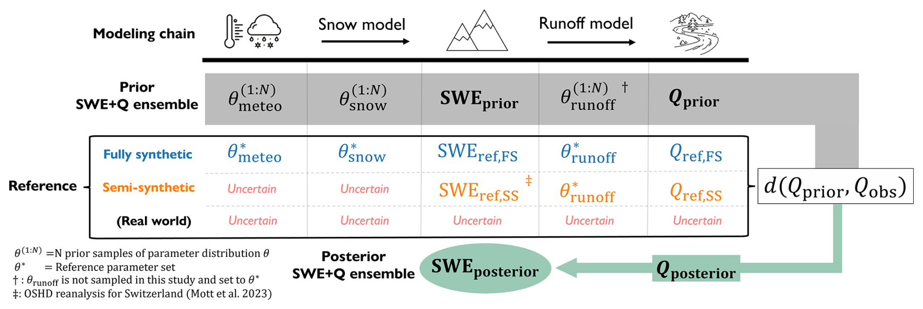
Figure 1 Schematic overview of the streamflow-constrained SWE reconstruction framework and the two synthetic numerical experiments. Q represents streamflow, θ represents the parameters to be sampled, θ^∗ represents the reference parameter set, and d represents the streamflow performance metric. Color-coding is consistent with the remainder of the study, with grey denoting the prior ensemble, green the posterior ensemble, blue the fully synthetic experiment (FS), and orange the semi-synthetic experiment (SS). See Sect. 2.2 for a detailed explanation of the workflow.

For each year between 2001 and 2022, 5000 model realizations are generated by randomly sampling parameter sets from uniform prior distributions $\mathrm{\Theta }=\mathit{\{}{\mathit{\theta }}_{\text{meteo}},{\mathit{\theta }}_{\text{snow}},{\mathit{\theta }}_{\text{soil}}\mathit{\}}$ using Latin Hypercube Sampling (Sect. 2.2.5). The resulting prior ensemble of simulated streamflow Q_sim is compared to observed streamflow Q_obs using a performance metric d(Q_sim,Q_obs), and the 1 % best-performing members are selected as the heuristic posterior ensemble (Sect. 2.4).

To test the methodology in a controlled environment, we evaluate it in two synthetic experiments: a fully synthetic case (FS; Sect. 2.3), which eliminates all modeling chain uncertainty, and a semi-synthetic case (SS), which adds meteorological and snow model structural uncertainty. The lower panel of Fig. 1 outlines the anticipated challenges for real-world applications, where additional uncertainty sources, particularly in the runoff model and streamflow observations, further complicate the inversion (Sect. 4.2).

2.2.1 Snow model

We use an enhanced temperature-index snow model that includes both air temperature and potential clear-sky radiation as melt drivers (Hock, 1999; Argentin et al., 2025). The model is implemented within the hydrological model wflow_sbm (van Verseveld et al., 2024, Sect. 2.2.2). Precipitation is partitioned into rainfall and snowfall using a melt temperature threshold T_thresh and a transition range as follows:

$$\begin{array}{}\text{(5)}& P_{\text{snow}}=\left\{\begin{array}{ll}P& \text{if }{T}_{\mathrm{a}}\le T_{\text{thresh}}-\mathrm{1}\\ P\cdot \left({\displaystyle \frac{\begin{array}{c}(T_{\text{thresh}}\\ +\mathrm{1})-T_{\mathrm{a}}\end{array}}{\mathrm{2}}}\right)& \begin{array}{l}\text{if }{T}_{\text{thresh}}-\mathrm{1}\\ <T_{\mathrm{a}}<T_{\text{thresh}}+\mathrm{1}\end{array}\\ \mathrm{0}& \text{if }{T}_{\mathrm{a}}\ge T_{\text{thresh}}+\mathrm{1}\end{array}\right.\end{array}$$

where P is precipitation and T_a represents air temperature in °C. We account for elevation-dependent biases in T_thresh using a linear lapse-rate correction:

$$\begin{array}{}\text{(6)}& T_{\text{thresh}}(x,y)=T_{\text{thresh}}+{\displaystyle \frac{{\mathit{\gamma }}_{T_{\text{thresh}}}}{\mathrm{1000}}}\cdot \left(z\right(x,y)-\stackrel{\mathrm{‾}}{z}),\end{array}$$

where (x,y) denote grid-cell coordinates, ${\mathit{\gamma }}_{T_{\text{thresh}}}$ is the temperature threshold lapse rate (°C km⁻¹), z(x,y) is grid-cell elevation, and $\stackrel{\mathrm{‾}}{z}$ is the catchment-mean elevation. Snowfall biases are corrected using a spatially uniform multiplicative correction factor c_snow combined with an elevation-dependent modulation γ_snow:

$$\begin{array}{}\text{(7)}& c_{\text{snow}}(x,y)=c_{\text{snow}}\cdot \left(\mathrm{1}+\stackrel{\mathrm{̃}}{z}(x,y)({\mathit{\gamma }}_{\text{snow}}-\mathrm{1})\right),\end{array}$$

where $\stackrel{\mathrm{̃}}{z}(x,y)$ is a dimensionless elevation coordinate defined as

$$\begin{array}{}\text{(8)}& \stackrel{\mathrm{̃}}{z}(x,y)={\displaystyle \frac{z(x,y)-\stackrel{\mathrm{‾}}{z}}{z_{\text{max}}-\stackrel{\mathrm{‾}}{z}}}\end{array}$$

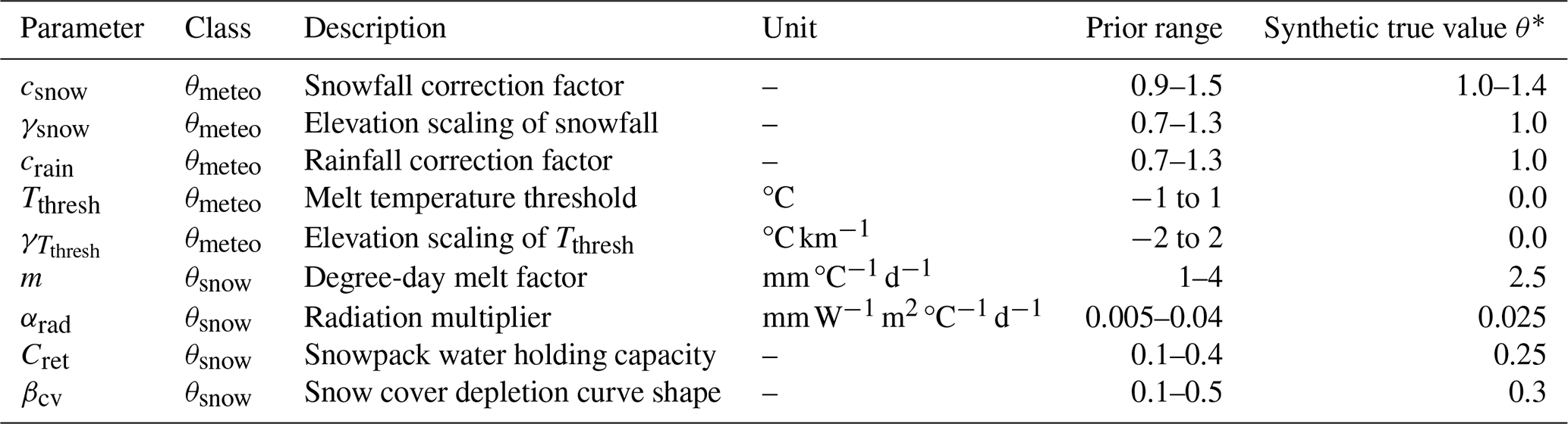
This formulation ensures non-negativity and equal but opposite adjustments of c_snow(x,y) above and below the catchment mean elevation. Note that a linear precipitation lapse rate does not account for potential capping of high elevation precipitation due to moisture depletion (Napoli et al., 2019). Liquid precipitation is calculated as P−P_snow and corrected separately using a spatially uniform rainfall correction factor c_rain (Sect. 2.2.4). The use of separate rainfall and snowfall correction factors is shown to improve meteorological bias correction in snow-dominated catchments (Pulka et al., 2024), and additionally allows us to assess whether the rainfall–snowmelt partitioning can be inferred from streamflow observations. The parameters c_snow, γ_snow, T_thresh, and ${\mathit{\gamma }}_{T_{\text{thresh}}}$ belong to the meteorological parameter set θ_meteo used to generate the prior SWE ensemble (Eq. 2 and Table 1).

Table 1 Overview of meteorological and snow model parameters used in the synthetic experiments. For details on the synthetic true parameter values, see Sect. 2.3.

Following the melt model introduced by Hock (1999), melt occurs when air temperature exceeds T_thresh, following:

$$\begin{array}{}\text{(9)}& F_{\mathrm{M}}\left(t\right)=\left\{\begin{array}{ll}\begin{array}{c}(m+{\mathit{\alpha }}_{\text{rad}}\cdot I_{\text{pot}})\\ \left(T_{\mathrm{a}}\right(t)-T_{\text{thresh}})\end{array}& \text{if }{T}_{\mathrm{a}}\left(t\right)>T_{\text{thresh}}\\ \mathrm{0}& \text{otherwise}\end{array}\right.\end{array}$$

where F_M is the melt rate (mm d⁻¹), m is the melt factor ($\mathrm{mm}{\mathrm{d}}^{-\mathrm{1}}\mathrm{°}{\mathrm{C}}^{-\mathrm{1}}$), α_rad is the radiation factor for snow or ice ($\mathrm{mm}{\mathrm{d}}^{-\mathrm{1}}\mathrm{°}{\mathrm{C}}^{-\mathrm{1}}{\mathrm{m}}^{\mathrm{2}}{\mathrm{W}}^{-\mathrm{1}}$) and I_pot is the potential clear-sky direct solar radiation (W m⁻²). We calculate I_pot for each grid cell based on the formula by Hock (1999) using the HydroBricks Python package (Horton and Argentin, 2024).

Meltwater is retained within the snowpack until it exceeds a calibratable water holding capacity (C_ret) fraction of the total snow mass (default: 0.1), after which drainage occurs. Liquid water may refreeze within the snowpack when T_a<T_thresh. Snow density evolution and rain-on-snow thermodynamics are not represented.

To represent sub-grid variability in snow depletion, we apply a fractional snow-covered area (f_SCA) parameterization based on Essery and Pomeroy (2004) and Magnusson et al. (2014):

$$\begin{array}{}\text{(10)}& f_{\text{SCA}}\left(t\right)=\tanh \left(\mathrm{1.26}\cdot {\displaystyle \frac{H_{{\text{SWE}}_{\text{sim}}}\left(t\right)}{{\mathit{\beta }}_{\text{cv}}\cdot H_{{\text{SWE}}_{\text{max}}}}}\right),\end{array}$$

where $H_{{\text{SWE}}_{\text{sim}}}$ is the simulated average SWE in the grid cell at time t, β_cv is the coefficient of variation, and $H_{{\text{SWE}}_{\text{max}}}$ is the pre-melt seasonal maximum SWE.

To account for snow redistribution by gravity, we implement a mass wasting scheme adapted from Frey and Holzmann (2015). Snow is redistributed to downhill cells as follows:

$$\begin{array}{}\text{(11)}& F_{\text{MW}}=\left\{\begin{array}{ll}\begin{array}{c}{c}_{\text{MW}}\cdot \text{min}\left(\mathrm{0.5},\frac{\mathit{\gamma }}{\mathit{\alpha }}\right)\\ \text{min}\left(\mathrm{1.0},\frac{H_{\text{SWE}}}{\mathit{\beta }}\right)\end{array}& \begin{array}{l}\text{if }{H}_{\text{SWE}}\\ >\mathrm{500}\wedge {\mathit{\rho }}_{\text{wet}}\\ <\mathrm{0.001}\wedge \mathit{\gamma }\\ >\mathrm{0.3},\end{array}\\ \mathrm{0}& \text{otherwise}\end{array}\right.\end{array}$$

where F_MW (mm d⁻¹) is the mass wasting flux per grid cell, c_MW (d⁻¹) is a correction factor set to 0.5, γ (–) is the slope, α (–) and β (–) are precalibrated factors set to α=5.67 and β = 10 000. ρ_wet (–) is the wet snow to dry snow ratio, which is a variable that our model outputs at every time step. m, α_rad, C_ret, and β_cv are retained as snow model parameters θ_snow used to generate the prior SWE ensemble (Eq. 2 and Table 1).

2.2.2 Runoff model

wflow_sbm (v0.7.1; van Verseveld et al., 2024) is an open-source, medium-complexity distributed hydrological model. While we adapted the wflow_sbm snow model (Sect. 2.2.1), we kept the runoff model intact. Each grid cell contains a vertically stratified soil column with up to four unsaturated layers and one saturated layer, allowing for dynamic water table movement. Soil hydraulic properties are inferred from global soil texture maps using pedotransfer functions (Imhoff et al., 2020).

For channel, overland, and lateral subsurface flow, the model uses the kinematic wave approach (van Verseveld et al., 2024). wflow_sbm uses globally available soil, vegetation, and terrain datasets, which are preprocessed using HydroMT (Eilander et al., 2023) (Table A1), and operates on a regular grid set to 30 arcsec resolution (approximately 900 m × 700 m at 40° latitude). We run wflow_sbm through the eWaterCycle hydrological modeling platform (Hut et al., 2022).

2.2.3 Test case: the Dischma catchment

The Dischma catchment in Switzerland spans 42.9 km² with elevations ranging from 1595 to 3180 $\mathrm{m}\mathrm{a}.\mathrm{s}.\mathrm{l}.$ (mean: 2372 m) (Fig. 2). The catchment is predominantly alpine, with minimal forest cover (∼ 3 %) and limited glacier extent (< 1 %). Beside cattle grazing, anthropogenic disturbances are negligible. Precipitation is fairly evenly distributed throughout the year, with roughly half falling as snow. Average annual discharge is 1229 mm yr⁻¹. The catchment has featured in numerous snow hydrological studies (Berghuijs et al., 2025; Brauchli et al., 2017; Comola et al., 2015; Schaefli, 2016), is actively monitored by the Swiss Federal Institute for Forest, Snow and Landscape Research (SLF; Magnusson et al., 2024), and is part of the CAMELS-CH dataset (Höge et al., 2023).

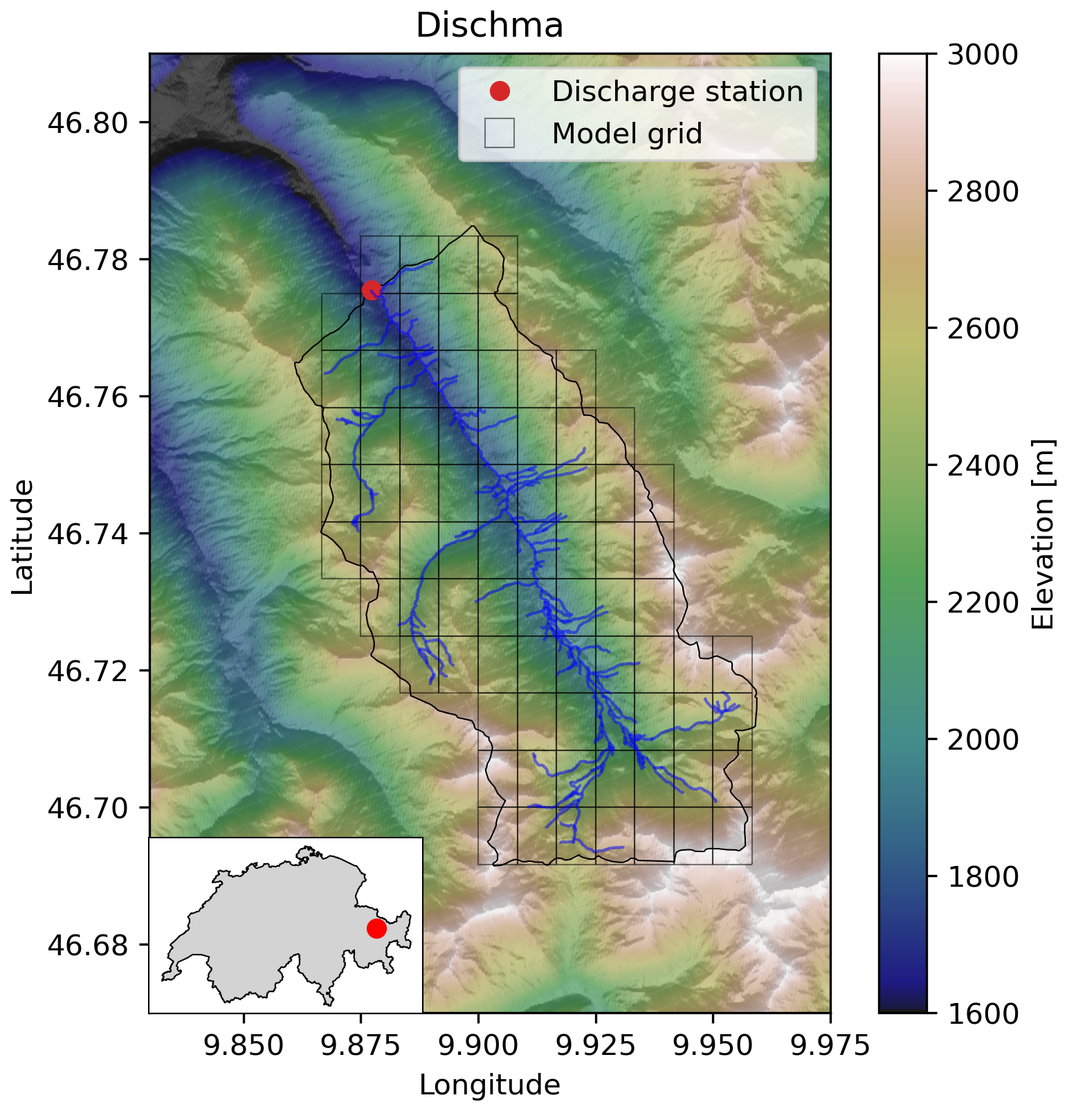
Figure 2 Digitial elevation model and delineation of the Dischma catchment, along with its location within Switzerland. The regular model grid has a resolution of 30 arcsec × 30 arcsec.

2.2.4 Meteorological forcing

Meteorological forcing data are obtained from MeteoSwiss and consist of gridded daily temperature (TabsD) and precipitation (RhiresD) estimates at 2 km × 2 km spatial resolution (MeteoSwiss, Federal Office of Meteorology and Climatology (2024), version 2.0). Both are based on station observations and use interpolation methods that account for topographic effects. The RhiresD dataset is known to suffer from gauge undercatch inherited from the station data (Magnusson et al., 2014). For the Dischma catchment, mean RhiresD precipitation across all grid cells is 1029 mm yr⁻¹ (1998–2022), which is in contradiction with observed streamflow of 1229 mm yr⁻¹ over the same period.

TabsD and RhiresD were downscaled to the 30 arcsec model grid using area-weighted regridding with ESMValTool (Eyring et al., 2020). TabsD was first adjusted to sea level using a fixed lapse rate of 6.5 °C km⁻¹ before regridding and then reprojected back to the original terrain elevation, while precipitation was regridded directly. For both coarse and fine resolution DEM we used the MERIT digital elevation model (Yamazaki et al., 2017). Potential and actual evapotranspiration were estimated using the semi-empirical method of de Bruin et al. (2016), which relies on shortwave radiation and near-surface air temperature.

2.2.5 Sampling strategy

As defined in Sect. 2.1, each parameter set Θ consists of meteorological parameters (θ_meteo), snow model parameters (θ_snow), and runoff model parameters (θ_runoff) (Eqs. 2 and 3). We restrict our analysis to synthetic experiments with complete knowledge of the runoff model structure and parameters. Consequently, θ_runoff is not subject to calibration and is fixed at default values as defined in the wflow_sbm documentation (Imhoff et al., 2020; van Verseveld et al., 2024) (Table B1). To generate the prior SWE and streamflow ensemble, we thus only sample from meteorological and snow model parameters θ_meteo and θ_snow (Table 1). Note that this approach is unsuitable when including θ_runoff, whose values likely vary little between years. A two-step sampling is then more suited, separating constant and annually varying parameters (Henn et al., 2015).

For each year between 2001 and 2022, 5000 parameter combinations are sampled from the joint prior parameter distributions of the 9 retained parameters using Latin Hypercube Sampling (LHS) (McKay et al., 2000), implemented through the SPOTPY Python package (Houska et al., 2015). While 5000 samples do not densely populate the prior parameter space, it is considered adequate for this study, as increasing the number of samples did not alter the results. We do not use an actual optimization algorithm or Markov Chain Monte Carlo sampling since the objective of our study is to explore the information content of streamflow for SWE inference by efficiently exploring the full parameter space rather than identifying the posterior distribution.

2.3 Synthetic numerical experiment design

To evaluate the constraining potential of streamflow for SWE reconstruction, we perform two synthetic experiments, both use the same prior ensemble of 5000 parameters described above.

2.3.1 Experiment 1: Fully synthetic (FS)

The first is an “inverse crime” experiment (Wirgin, 2004): we generate synthetic SWE and streamflow using the same snow and runoff model structures as those used for inversion, ensuring consistency between forward and inverse models. In doing so, we aim to quantify the theoretical potential of streamflow-constrained SWE inversion by eliminating any model structural error or observation uncertainty. The synthetic true parameters θ^∗ used to generate synthetic SWE (SWE_ref,FS) are given in Table 1. The snowfall correction factor oscillates over all years between 1 and 1.4, with annual changes of 0.1. This mimics the full potential extent of seasonal meteorological forcing bias. For the remaining parameters, θ^∗ is set to the midpoint between the lower and upper prior bounds. Because LHS ensures uniform coverage of each parameter's range, the median of the sampled parameter set Θ will approximate θ^∗. Consequently, the ensemble mean of the resulting prior SWE simulations SWE_prior is expected to roughly approximate the reference simulation SWE_ref,FS.

2.3.2 Experiment 2: Semi-synthetic (SS)

The second experiment is a semi-synthetic experiment, where we use the Swiss temperature-index SWE reanalysis product OSHD (Mott et al., 2023; Mott, 2023) as the synthetic SWE reference SWE_ref,SS. This product combines a temperature-index snow model with data assimilation of in-situ SD observations for both snowfall and SWE state correction. It is available for all of Switzerland since 1998 at 1 km resolution. Although the underlying meteorological forcing is comparable to that used in this study, the combination of an alternative model structure and assimilation-induced SWE corrections introduces both snow model and meteorological deviations relative to the base snow model and forcing. This introduces artificial snow-related uncertainty in the inversion, thereby making it closer to real-world conditions (Fig. 1). The semi-synthetic experiment thus allows us to examine the degradation in inversion performance when realistic discrepancies exist between the “true” and assumed snow processes. To establish the coupling between OSHD and wflow_sbm, the OSHD output is first resampled to the wflow_sbm grid and then inserted in the wflow_sbm model by modifying the meteorological forcing: all snowfall events (i.e., P when T_air < 0 °C) are removed, OSHD-derived snowmelt is added as precipitation, and air temperature is capped at a minimum of 0 °C to ensure this precipitation falls as rain. Testing of this coupling approach showed that the secondary effects of capping the temperature at 0 °C are negligible. The runoff model and streamflow observations remain without uncertainty, isolating the impact of snow-related uncertainties. Rainfall correction factor c_rain is not dictated by OSHD and is still inferred, with the true c_rain ($c_{\text{rain}}^{\ast }$) set to 1. The rainfall correction is applied only to the RhiresD forcing, not to the OSHD-derived snowmelt implemented as rainfall.

2.4 Posterior ensemble selection

We use the Nash–Sutcliffe Efficiency (NSE, Nash and Sutcliffe, 1970) as the streamflow performance metric to quantify agreement between model output and observations (denoted as E_Q-NSE). An NSE of 1 indicates perfect agreement, while an NSE of 0 implies no improvement over using the observed mean as a predictor. We calculate NSE over the snowmelt season (March to July) to focus on snowmelt-driven discharge. Although NSE can give inflated values in catchments with strong seasonality, such as the Dischma (Schaefli and Gupta, 2007), our focus is on relative differences in NSE, reflecting variations in squared error magnitudes.

We adopt a rank-based heuristic posterior selection. All prior ensemble members are evaluated against observed streamflow using NSE, and the top 1 % are selected as the posterior ensemble, yielding a posterior size of N_posterior = 50. The quality of this posterior ensemble is then evaluated on different SWE metrics (Sect. 2.5).

2.5 Posterior SWE evaluation

2.5.1 SWE metrics and scales

We evaluate SWE reconstructions using a set of performance metrics that target different physical properties of the seasonal snowpack. We follow the concept of the “snow triangle” metrics from Trujillo and Molotch (2014) and Rhoades et al. (2018), with modifications. Unlike Rhoades et al. (2018), who reduce snowfall and melt to seasonal means, we use the daily time series of snowfall and melt to better evaluate temporal dynamics and individual events. For snow accumulation, we use the sum of seasonal snow accumulation rather than peak SWE volume, to reflect the total snow contribution to the catchment water balance. We include the dates of SWE onset and melt-out but omit other timing metrics, such as date of peak SWE and melt season length, as their information is assumed to be embedded in the remaining metrics. Each performance metric E is computed annually at two spatial scales:

• Catchment-aggregated (AGG): E_AGG metrics are calculated from the spatially averaged SWE time series across the catchment.

• Distributed (GRID): E_GRID metrics are computed per grid cell and averaged over space.

This allows assessment of whether streamflow informs the spatial structure or only the integrated behavior of the snowpack. Such multi-scale evaluation is enabled by full spatio-temporal availability of the reference SWE.

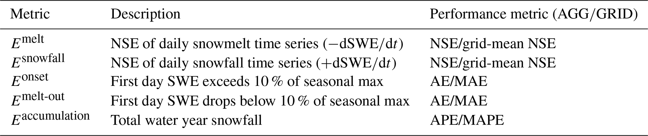
Each performance metric matches the nature of the evaluated variable (Table 2). For the evaluation of time series (melt and snowfall), we use the NSE (Sect. 2.4) in AGG mode, and the grid-mean NSE in GRID mode. For total accumulation, we use Absolute Percentage Error (APE) in AGG mode and Mean Absolute Percentage Error (MAPE) in GRID mode. For timing metrics evaluating SWE onset and melt-out dates, we express the dates in day-of-year and use Absolute Error (AE) in AGG mode and Mean Absolute Error (MAE) in GRID mode.

Table 2 Overview of SWE performance metrics used to evaluate the streamflow-derived posterior SWE ensemble. Error types are given for catchment-aggregated (AGG) and distributed (GRID) modes.

2.5.2 Posterior rank evaluation

To assess how well streamflow constrains SWE, we apply a rank-based diagnostic. All 5000 prior members are ranked on each performance metric. We then identify the ranks of the 50 posterior ensemble members in this list and compute their median rank, denoted R_post,median.

If streamflow perfectly selects the best SWE scenarios, we expect R_post,median = 25, corresponding to the median of 50 samples (rounded down from 25.5). Conversely, if streamflow offers no useful constraint, posterior members will be randomly distributed throughout the prior, and R_post,median = 2500, corresponding to the median rank among 5000 samples (rounded down from 2500.5). A median rank significantly higher than 2500 would suggest streamflow-based selection degrades performance for that metric. Note that this rank-based summary neglects the distribution shape of posterior ranks, focusing solely on the median.

3 Results

3.1 Posterior parameter ensembles

The inferred posterior parameter ensembles do not consistently align with the true parameter values in the FS experiment (Fig. 3a and b). Among all parameters, c_snow is the most sensitive. Its annual posterior values generally reflect the imposed artificial bias fluctuations $c_{\text{snow}}^{\ast }$, but still span a wide range. For example, in 2001 where $c_{\text{snow}}^{\ast }$ = 1, posterior values range from approximately 0.9 to 1.3, implying that both a 10 % underestimation and a 30 % overestimation of total snowfall can result in high streamflow skill. The remaining parameters are considerably less sensitive and generally span most of their prior ranges, equally indicating that a wide range of SWE realizations can produce similarly high-performing streamflow responses and suggesting compensating behavior among parameters.

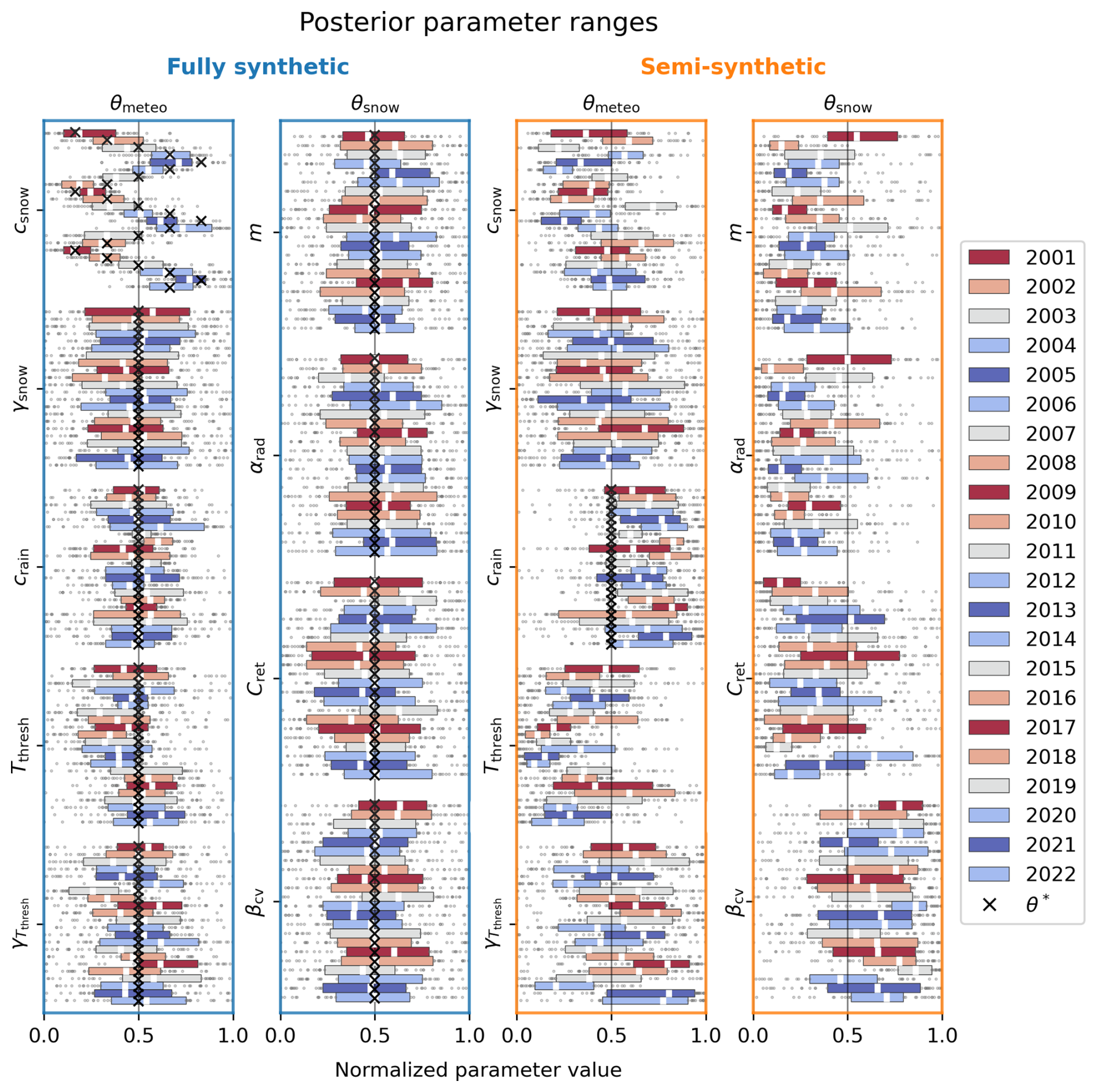
Figure 3 Annual posterior parameter ensembles for the FS and SS experiments, expressed relative to the normalized prior range. θ_meteo and θ_snow represent the meteorological and snow model parameters. Medians (white squares), interquartile ranges (boxes), and lower- and upper-quartile values (grey dots) are shown for the 50 posterior parameter values. The true parameter values used to generate the synthetic observations (θ^∗) are represented by black crosses. The color-coding is based on the annually fluctuating values of $c_{\text{snow}}^{\ast }$ in FS.

In the SS experiment, of all true parameter values Θ^∗ only $c_{\text{rain}}^{\ast }$ is imposed. The true value of the remaining parameters is unknown, as the reference SWE is an external product. Figure 3c shows that c_rain is consistently overestimated, which is compensated by an annual underestimation of catchment-wide SWE accumulation of 6.6 ± 4.4 %. The posterior c_snow values vary widely across the prior range, suggesting annually varying biases in the snowfall forcing and confirming the need for annual rather than multiannual inversion. The values of T_thresh, m, r and C_ret are generally on the lower edge of the prior range, while ${\mathit{\gamma }}_{T_{\text{thresh}}}$ and β_cv are generally on the higher edge. This suggests slower melt taking place preferentially at higher elevations, lower water holding capacity, and faster snow cover depletion of SWE_ref,SS (i.e. OSHD-TI product) compared to our prior assumptions.

3.2 Streamflow and SWE performance

In the previous section, we showed that we cannot reliably recover the true parameter values from streamflow alone, with NSE as the streamflow performance metric. To better understand this result, we analyze the model performances associated with the best ranked parameter sets. Figure 4 shows the E_Q-NSE results and posterior ensemble selection (Fig. 4a and c) and the subsequent evaluation of this selection on $E_{\text{GRID}}^{\text{accumulation}}$ (Fig. 4b and d), for both FS and SS. We show $E_{\text{GRID}}^{\text{accumulation}}$ results as it is arguably the most relevant performance metric for gridded SWE reconstructions. The results for other target SWE metrics are presented in Figs. S1–S10 in the Supplement.

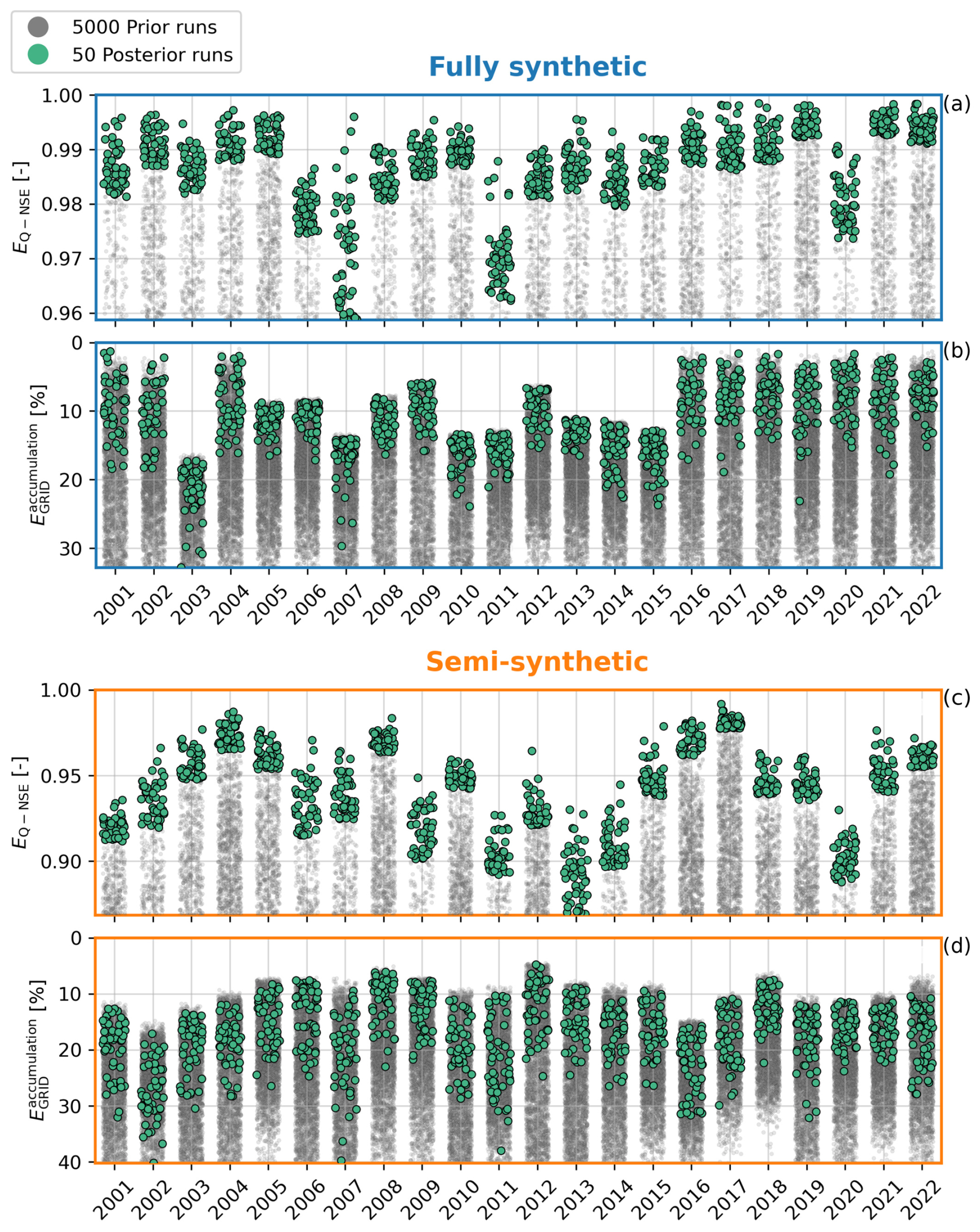
Figure 4 NSE-based posterior selection (a, c) and grid-mean total snowfall mismatch ($E_{\text{GRID}}^{\text{accumulation}}$) of all model runs (b, d), for both FS (a, b) and SS (c, d) experiments. Grey points represent the 5000 annual prior members (above the y-axis cutoff), while green points represent the posterior ensemble, i.e. the 50 members with the best streamflow performance.

The E_Q-NSE results confirm strong agreement between simulated and synthetic streamflow in both experiments, with an overall mean posterior NSE of 0.99 ± 0.01 for FS, and 0.94 ± 0.03 for SS (Fig. 4a and c), compared to an overall mean prior NSE of 0.67 ± 0.11 for FS and 0.56 ± 0.16 for SS. $E_{\text{GRID}}^{\text{accumulation}}$ results reach maximum scores of near 0 % in FS in some years, while not exceeding 10 % in most other FS and SS years. This is likely due to a combination of high sensitivity of the highest and lowest elevation grid cells to the γ_snow and ${\mathit{\gamma }}_{T_{\text{thresh}}}$ parameters, and the fact that in the SS experiment a perfect approximation of the external SWE product is generally not possible.

Across both experiments, posterior members generally occupy the lower-error portion of the prior distribution, indicating that streamflow provides a meaningful constraint on gridded SWE accumulation. However, many prior members outperform the posterior ensemble, demonstrating that high streamflow skill does not uniquely translate into high spatial SWE accumulation skill. The strength of this constraint varies between years, with some years showing a narrow spread and others showing a wide spread among the posterior ensemble.

3.3 Posterior rank evaluation across SWE metrics

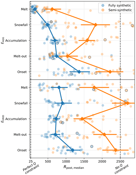
Across both experiments, $E_{\text{AGG}}^{\text{melt}}$ is the most strongly constrained metric among all SWE metrics, indicating that streamflow most effectively constrains catchment-scale melt dynamics (Fig. 5). In FS, R_post,median values lie close to the perfect-constraint limit in most years, whereas in SS they are substantially higher and more variable, reflecting reduced identifiability under added forcing and model uncertainty. In contrast, $E_{\text{GRID}}^{\text{melt}}$ is only weakly constrained in both experiments, indicating that while streamflow constrains integrated melt production, it provides limited information on its spatial origin.

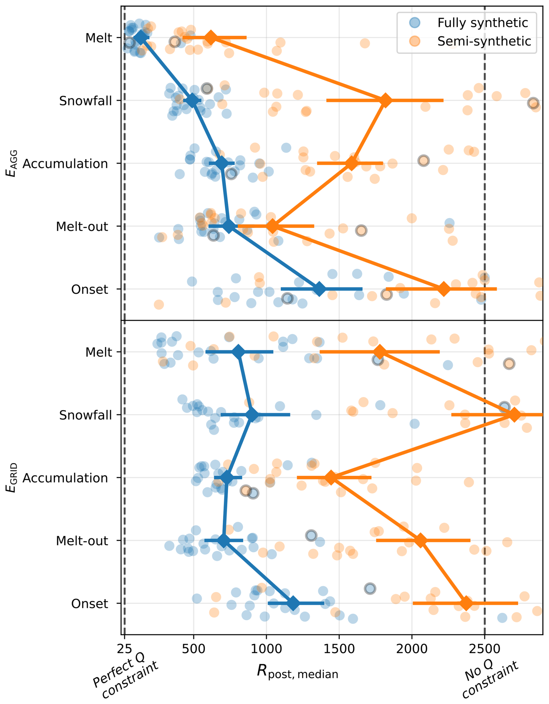
Figure 5 Annual median SWE metric ranks of the streamflow-derived posterior ensembles, relative to all 5000 prior members. The top figure shows the results for catchment-aggregated SWE metrics (E_AGG), while the bottom shows grid-averaged metrics (E_GRID), sorted based on the FS E_AGG ranks. Each point represents the annual median posterior rank between 2001–2022, with the year 2003 in thick outline as an example. The diamonds represent the mean of all median posterior ranks, and the error bars represent the 95 % confidence interval. The fully and semi-synthetic experiments are represented in blue and orange, respectively. The definitions of the error metrics are given in Sect. 2.5.1.

Snowfall-related metrics are more weakly and inconsistently constrained. In FS, both $E_{\text{AGG}}^{\text{snowfall}}$ and $E_{\text{GRID}}^{\text{snowfall}}$ show moderate constraint, likely benefiting from the same parameter sets that favor melt performance. In SS however, both metrics are weakly constrained, confirming the limited ability of streamflow to inform snowfall dynamics when accumulation and melt biases differ.

Accumulation metrics show intermediate constraint. $E_{\text{GRID}}^{\text{accumulation}}$ is more strongly constrained than $E_{\text{AGG}}^{\text{accumulation}}$ in both experiments, suggesting that the spatial distribution of snow accumulation is equally or better constrained by streamflow than the total catchment-wide accumulation. Note, however, that a different streamflow performance metric than NSE (e.g. seasonal streamflow bias) might favor the constraint of catchment-aggregated accumulation more (Sect. 4.3).

Among timing metrics, melt-out dates are relatively well constrained, particularly in AGG mode. This is consistent with their physical link to the cessation of snowmelt-driven streamflow. In contrast, SWE onset dates are weakly constrained across experiments and scales.

Overall, constraints are systematically weaker and more heterogeneous in SS than in FS. R_post,median increases by 989 on average across all metrics, corresponding to 20 % of N_prior, while its standard deviation increases on average by 414. This confirms that the added structural and input uncertainty in SS reduce the ability of streamflow to constrain SWE. Additionally, the increased spread in R_post,median across different SWE performance metrics in SS indicates that members performing well on one metric no longer consistently perform well on others. This suggests a decoupling of performance among metrics and growing trade-offs between competing aspects of SWE reconstruction under added uncertainty. Nonetheless, except for $E_{\text{GRID}}^{\text{snowfall}}$ in SS, most median ranks remain above the no-constraint threshold.

3.4 Correlation among metrics

To assess the complementarity of the retained SWE metrics, Fig 6 shows the Spearman rank correlation between all SWE performance metrics and streamflow NSE across the full prior ensemble for each year. Consistent with previous results, $E_{\text{AGG}}^{\text{melt}}$ is the SWE metric most strongly associated with E_Q-NSE in both experiments (ρ_FS = 0.89, ρ_SS = 0.63). Overall, correlations are systematically stronger in FS than in SS, and catchment-aggregated metrics generally correlate well with their gridded counterparts. While $E_{\text{AGG}}^{\text{melt}}$ correlates the strongest with E_Q-NSE, correlation of other SWE metrics with catchment-aggregated melt does not translate to strong correlation with E_Q-NSE as well. It is the case for E^melt-out, but not for $E_{\text{GRID}}^{\text{melt}}$. These results suggest that, in general, streamflow contains information about different SWE metrics independently. In other words, the posterior members performing well on one SWE metric do not necessarily perform well on others. This supports the use of multiple, complementary SWE metrics and cautions against drawing conclusions from any single metric.

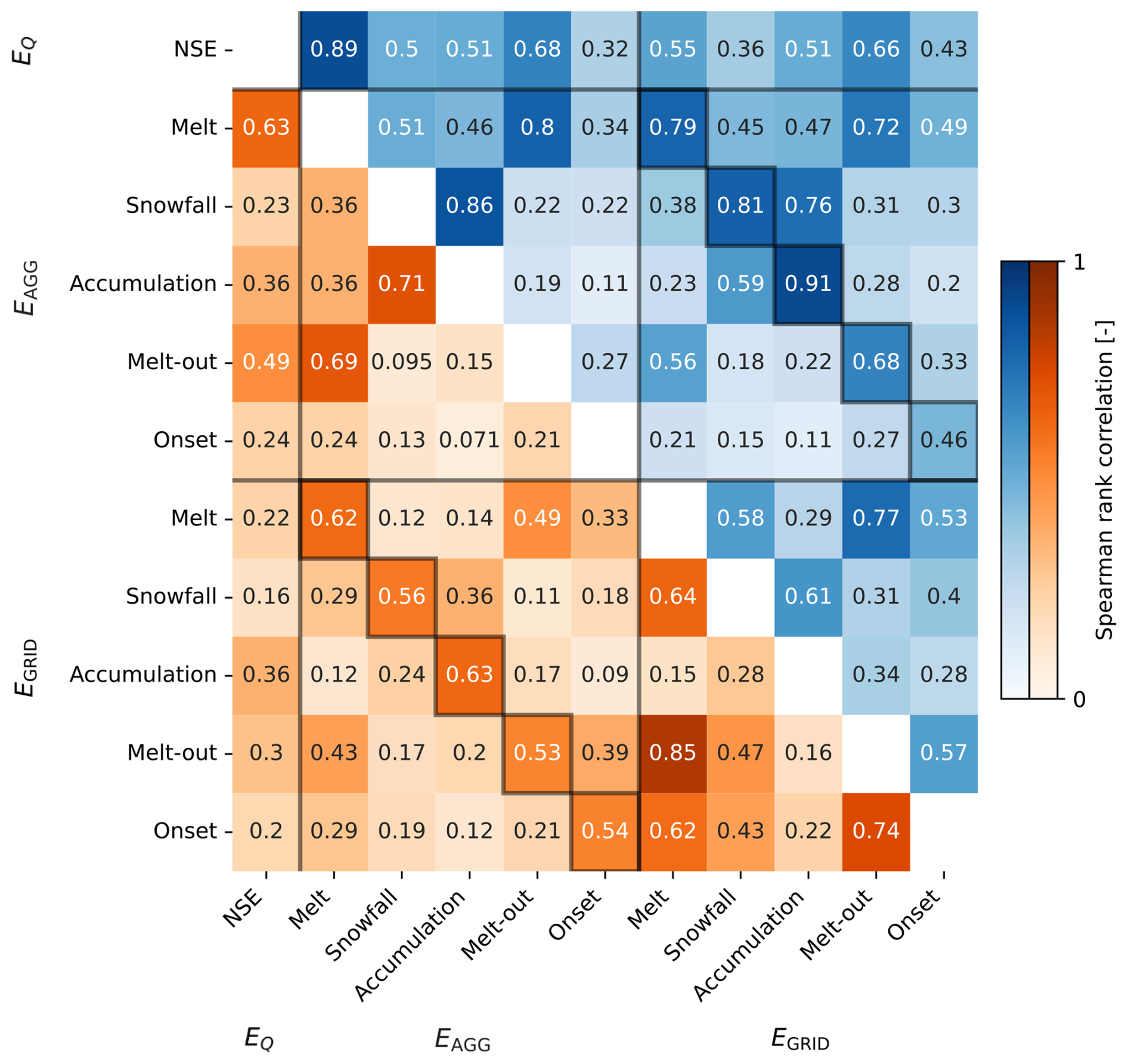
Figure 6 Correlations among all retained streamflow and SWE performance metrics, expressed as the median of annual Spearman rank correlations over all 5000 yearly prior members between 2001 and 2022. The upper values in blue represent the fully synthetic experiment, while the lower values in orange represent the semi-synthetic experiment. Black lines delineate streamflow (Q), catchment-aggregated SWE (E_AGG), and spatially distributed SWE (E_GRID) performance metrics. Black squares emphasize E_AGG-E_GRID diagonals.

4 Discussion

4.1 Streamflow constraining potential under idealized conditions

The fully synthetic experiment confirms that streamflow-constrained SWE inversion works in theory, but near-perfect constraint is only achieved for catchment-aggregated melt. Other SWE properties generally remain well-constrained, but far from perfectly constrained. We hereby demonstrate that even under highly idealized conditions, streamflow does not consistently identify the best-performing SWE scenarios across all performance metrics. This finding is mainly explained by physical non-uniqueness in the SWE-streamflow relationship (Beaton et al., 2024): different SWE and rainfall scenarios can lead to equivalent streamflow responses. Catchment-aggregated melt being better constrained than distributed melt is a first indication of this, by showing that biased spatial melt distributions can lead to an accurate aggregated melt output. A second indication is given by the imperfect constraint on catchment-aggregated accumulation: the best-performing streamflow performance can be achieved with biased catchment-wide SWE accumulation estimates. Finally, we show that multiple distinct SWE and rainfall combinations can yield similar streamflow responses (Fig. 3 and Sect. 3.1).

A second source of uncertainty in the FS experiment is structural non-uniqueness or equifinality (Beven and Freer, 2001; Günther et al., 2020), whereby multiple parameter sets yield similar SWE outcomes. However, since this study focuses on SWE performance rather than parameter convergence, such equifinality is not of major concern. A third potential source is parameter estimation uncertainty, i.e., the failure to identify optimal parameter combinations by the sampling algorithm. Yet this is also of minor importance, as the posterior simulations already achieve high streamflow skill, and further optimization or a different $N_{\text{posterior}}/N_{\text{prior}}$ ratio would not affect the SWE-streamflow relationships central to our analysis.

The semi-synthetic experiment shows that adding meteorological and snow model uncertainty significantly reduces the ability of streamflow to constrain SWE across all performance metrics. This reduction suggests a mismatch between our meteorological forcing and snow model versus the OSHD reference that the current inversion framework is unable to correct. Alongside physical non-uniqueness, uncertainties throughout the modeling chain thus present an additional barrier to accurately identifying realistic SWE scenarios from streamflow. These added uncertainties also introduce stronger trade-offs between SWE metrics: even when the best-performing ensemble members for one SWE metric are correctly identified, they are less likely to perform well on other SWE performance metrics.

4.2 Additional challenges under real-world conditions

Under real-world conditions, constraining SWE reconstructions using streamflow presents additional challenges beyond the idealized setup explored in this study. These challenges include both substantially increased uncertainty and reduced opportunities for performance evaluation (Fig. 1). One major source of uncertainty not addressed here is runoff model uncertainty. This encompasses both uncertainty in static catchment properties and uncertainty in the representation of water transport processes through the catchment (Beven, 2006). Such uncertainty can introduce persistent timing biases in the translation of snowmelt into streamflow, thereby complicating efforts to infer SWE dynamics from streamflow observations (Henn et al., 2018). Additional uncertainty arises from streamflow observations, including errors in stage measurements, discharge gauging, rating curve estimation (Di Baldassarre and Montanari, 2009), and ice-related effects (Burrell et al., 2023), which can propagate into both event-scale timing errors and biases in seasonal water balance estimates. Finally, the meteorological and snow model uncertainties imposed in the semi-synthetic experiment are likely to be conservative relative to real-world conditions. In practice, meteorological forcing errors are expected to be larger, not least due to the addition of evaporation estimation uncertainty, and snowpack dynamics are more heterogeneous and complex than represented by the OSHD model. Taken together, these additional sources of uncertainty are expected to further diminish the constraining potential of streamflow on SWE reconstruction beyond the reduction observed here between the fully synthetic and semi-synthetic experiments.

An additional challenge in real-world applications is the lack of long-term, temporally continuous and catchment-scale SWE observations against which to evaluate inversion results (Revuelto et al., 2025). Unlike in our synthetic experiments, real-world evaluations forcibly rely on spatially or temporally incomplete observations, making it inherently difficult to assess whether the SWE inversion was successful. At present, the best evaluation dataset is arguably the biweekly gridded SWE product of the Airborne Snow Observatory (Painter et al., 2016), available for a limited number of catchments and years in the Western US. The lack of evaluation data equally implies a lack of training data for data-driven methods, thereby limiting the potential of machine learning methods as an alternative link between SWE and streamflow in inverse hydrological SWE reconstruction. A practical way forward is to continue refining idealized experiments by further adding controlled sources of uncertainty, such as runoff model and streamflow observation errors, thereby approximating real-world complexity while retaining the ability to assess inversion effectiveness quantitatively.

4.3 Potential inversion framework adaptations

Several elements of the inversion framework proposed here may require adaptation under real-world conditions, where uncertainty is higher and evaluation opportunities are more limited. One key limitation is the use of NSE as the streamflow performance metric. NSE is highly sensitive to timing errors, potentially penalizing simulations that reproduce melt events with small temporal shifts more strongly than simulations that miss them entirely. This sensitivity is particularly relevant given our finding that streamflow most strongly constrains catchment-aggregated melt, which is inherently timing-dependent. In addition, as a residual-based metric, NSE may preferentially favor parameter sets that perform well on residual-based SWE metrics, while disadvantaging those that perform better on bias-based SWE metrics. Alternative streamflow metrics targeting hydrological signatures, such as variability or seasonal volume (Schaefli, 2016), may therefore provide more robust constraints under real-world uncertainty. Consequently, the results presented here should be considered strictly in light of the use of NSE as the streamflow performance metric. A full analysis of the streamflow and SWE performance metric interactions is outside the scope of this work, but is recommended for future research.

Given the increased spatial and temporal variability of meteorological forcing in real-world applications, the simple bias-correction factors used here (θ_meteo) are likely insufficient. In reality, snowfall, rainfall and melt biases vary at sub-seasonal and event time scales, and elevation dependencies are often non-linear in complex terrain. Allowing for greater temporal flexibility and spatial heterogeneity in the correction of meteorological biases may therefore improve the identifiability of relevant SWE processes from streamflow observations, albeit at increased computational cost.

Finally, the choice of snow and runoff models is likely to influence inversion performance. While relatively simple snow models can perform well at the catchment scale (Magnusson et al., 2015), more physically based formulations may be better suited where meteorological data are abundant (Mott et al., 2023). In contrast, the inversion could benefit from decreased complexity in the runoff model. Since the primary function of the runoff model in this framework is to translate spatial melt into streamflow, semi-distributed or lumped models could reduce computational costs and allow for larger ensembles compared to the fully distributed runoff model used here. More broadly, employing multiple snow and runoff models within the inversion framework could enhance robustness by better accounting for structural model uncertainty and increasing the likelihood of capturing realistic SWE evolution and snowmelt runoff.

4.4 Outlook on the added value of streamflow in SWE reconstructions

Under real-world conditions, streamflow alone may fail to reliably distinguish biased from unbiased SWE simulations. In the absence of reliable SWE evaluation data, the streamflow-based selection of biased SWE simulations might even go undetected. This implies that streamflow may, in some cases, not provide added value compared to simply running a snow model with uncorrected meteorological forcing. Several factors determine whether streamflow is likely to provide added value for SWE reconstruction. First, the quality of meteorological observations is crucial. Low meteorological biases result in low biases in SWE reconstructions, reducing the need for streamflow to constrain them. Secondly, the size, shape, and climate of the target catchment play a role. Smaller, elongated catchments (e.g. the Dischma catchment of this study) exhibit lower non-uniqueness than large, round catchments (Rinaldo et al., 1995), while snow-dominated catchments offer better identifiability of snowmelt than snow-scarce catchments (Griessinger et al., 2016). Dry spring and summer climates particularly benefit streamflow-assisted SWE inversion as they limit the confounding between rainfall and snowmelt signals (Henn et al., 2015). The same logic likely also applies to inter-annual variability within each catchment. In years with higher snowfall fractions and less spring rainfall, streamflow likely has greater constraining potential on SWE reconstructions. The above factors favor the application of streamflow-assisted SWE inversion as far back as streamflow observations allow, as meteorological forcing products have become less biased (Kouki et al., 2023), and snowfall dominance has decreased with time (Han et al., 2024). They also favor its application to meteorologically under-observed mountain regions such as the Himalayas and the Andes, where forcing products equally tend to be more biased and SWE evaluation is scarcer (Beck et al., 2019; Thornton et al., 2021). While this study focuses on mountainous catchments, it would be valuable to assess the constraining potential of streamflow in lower-relief, less topographically complex environments such as boreal catchments, where different controls on snow accumulation and melt may lead to different identifiability of SWE dynamics in streamflow.

In this study, we isolate the constraining potential of streamflow alone. However, streamflow is likely most effective when used in combination with other sources of snow information. These can be direct observations of different snow properties (Revuelto et al., 2025), but we particularly encourage future work to explore the use of recurring spatial patterns of snow dynamics (Vögeli et al., 2016; Pflug and Lundquist, 2020; Geissler et al., 2025). Such patterns represent catchment-specific prior knowledge that, once characterized, can be reused across time, including periods predating satellite observations but overlapping streamflow observations. Prior SWE ensembles could be defined as scaled versions of present-day observed spatial SWE patterns, thereby reducing the number of parameters to be inferred and mitigating part of the physical non-uniqueness identified in this study. Alternatively, the recurring patterns could be used to filter posterior SWE members based on physical plausibility. So far, these recurring patterns have been characterized in a limited number of catchments, but recent advances in automated UAV and LiDAR technologies are likely to increase this number in the near future (Revuelto et al., 2021). Combined with long streamflow records, this opens the possibility of extending SWE reconstructions back in time by decades while maintaining realistic spatial SWE patterns.

Regardless of the accompanying information source, streamflow remains a unique source of snow information in its ability to capture catchment-integrated SWE dynamics, most notably the timing and total volume of snowmelt runoff. Our finding that streamflow most effectively constrains catchment-aggregated melt supports its potential role in this context. In light of results by Rhoades et al. (2018), who showed that many SWE products systematically misrepresent average melt rates in mountainous terrain, streamflow is the only observational source capable of directly constraining such errors at the catchment scale. We therefore propose that future studies investigate the integration of streamflow with other snow data sources to constrain SWE reconstructions as much as practically possible.

5 Conclusion

We presented a framework for streamflow-constrained SWE reconstruction at the catchment scale using inverse hydrological modeling. We tested the methodology in two synthetic numerical experiments and across five target SWE metrics calculated on both catchment-aggregated and spatially distributed scales. The fully synthetic experiment showed that, even in the absence of all modeling chain uncertainty, a range of different SWE realizations and snowmelt/rainfall combinations can lead to equivalent and very high-performing streamflow estimates. The semi-synthetic experiment showed that the addition of artificial meteorological and snow model uncertainty leads to a considerable reduction in the constraining potential of streamflow across all SWE properties. In both experiments, streamflow has the most constraining potential on catchment-aggregated melt, although this finding is conditional to the use of NSE as the streamflow performance metric. Overall, this study showed that even in synthetic experiments devoid of observation and runoff model uncertainty, the relationship between streamflow and SWE properties is complex and non-linear, and streamflow alone can only constrain SWE reconstructions to a limited degree. We therefore expect streamflow-constrained SWE reconstructions using the presented framework to be challenging in many real-world cases, when the issues of non-uniqueness and uncertainties across the modeling chain are further amplified. We suggest future studies to explore the combined use of streamflow with other sources of snow information, across diverse catchments and using a wider range of streamflow performance metrics.

Appendix A: HydroMT global datasets

Karger et al. (2017)Kottek et al. (2006)Yamazaki et al. (2017)Yamazaki et al. (2019)Myeni et al. (2015)Poggio et al. (2021)Buchhorn and smets (2020)

Table A1 Global datasets used to setup wflow through the HydroMT package.

Appendix B: wflow_sbm default parameters

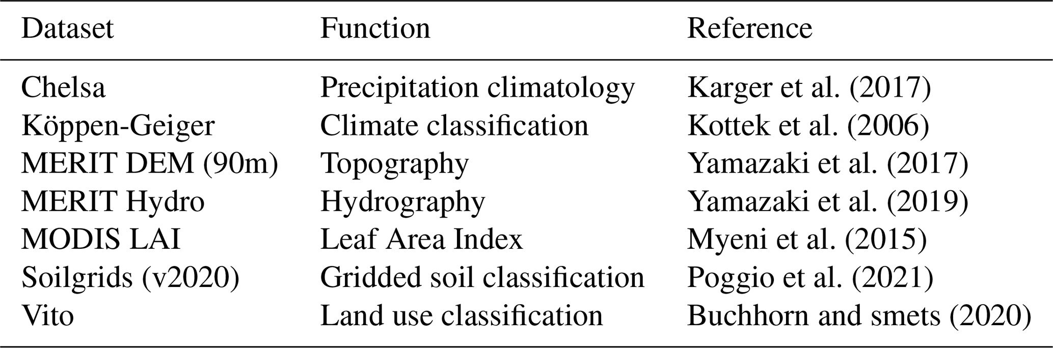
Table B1 Key wflow_sbm parameters used in this study. All parameters are unitless. For the remaining parameter values, we refer to van Verseveld et al. (2024).