High resolution monthly precipitation isotope estimates across Australia from machine learning

The stable isotopic composition of precipitation (δ²H_P, δ¹⁸O_P; “water isotopes”) is a powerful tool for tracking water through the atmosphere, as well as fingerprinting land-surface water masses and identifying water cycle biases in isotope-enabled climate models. Water isotopes also underpin our understanding of multi-decadal to multi-centennial water cycle variability via their retrieval from palaeoclimate archives. Water isotopes thereby increase our understanding of past and present – and hence future – water cycle variability. Understanding the drivers of spatial and temporal water isotope variability is a critical first step in applying these tracers for a better understanding of the water cycle. However, water isotope observations are sparse in both space and time. Here we develop and apply a machine learning (random forest) approach to predict spatially continuous monthly δ²H_P and δ¹⁸O_P across the Australian continent at 0.25° resolution from 1962–2023. We train the random forest models on monthly δ²H_P (n=5199) and δ¹⁸O_P (n=5217) observations from 60 sites across Australia. We also predict the deuterium excess of precipitation (dxs_P, defined as δ²H${}_{\mathrm{P}}-\mathrm{8}\times {\mathit{\delta }}^{\mathrm{18}}$O_P). Out-of-sample δ²H_P and δ¹⁸O_P prediction skill is high both geographically and temporally. Skill is slightly lower for the secondary parameter dxs_P, likely reflecting the larger reliance of spatio-temporal dxs_P variability on moisture source conditions. The random forest models accurately capture both the seasonal cycle of precipitation isotopic variability and long-term annual-mean precipitation isotopic variability across the continent, and outperform estimates from an isotope-enabled atmosphere general circulation model over an equivalent time period. We show that spatio-temporal variability in precipitation amount, precipitation intensity, and surface temperature are particularly important for monthly δ²H_P and δ¹⁸O_P variations across the continent, with local surface pressure also important for dxs_P. Drivers of site-level δ²H_P, δ¹⁸O_P, and dxs_P are more varied. Overall, the new random forest modelled dataset reveals clear spatial and temporal variability in δ²H_P, δ¹⁸O_P, and dxs_P across the Australian continent over the past decades – providing a robust foundation for hydrology, ecology, and palaeoclimate research, as well as an accessible framework for predicting water isotope values in other locations.

1 Introduction

The stable isotopic composition of precipitation (δ²H_P, δ¹⁸O_P¹) is an integrative tracer of the dynamical processes resulting in a particular amount of precipitation falling in a particular place at a particular time (Bowen et al., 2019; Galewsky et al., 2016). Water molecules comprising only the common light (¹H, ¹⁶O) isotopes have higher saturation vapour pressures than water molecules containing a rarer heavy (²H, ¹⁸O) isotope. Consequently, a mass-dependent isotopic fractionation occurs every time water changes phase (evaporation, condensation, sublimation, riming). For example, when water vapour condenses to liquid, water molecules with heavy isotopes will preferentially go to the liquid phase relative to those with light isotopes. The magnitude of equilibrium fractionation depends on the ambient temperature (Majoube, 1970, 1971). Diffusive processes impart additional kinetic fractionation, resulting in important impacts from, for example, ambient relative humidity and the time available for isotopic equilibration between the two phases (Galewsky et al., 2016). Hence, information about any process involving a water phase change is recorded in the stable isotope composition of a moisture parcel as it moves through the atmosphere, and may be preserved in the ultimate isotope composition of surface precipitation. These water cycle processes include (but are not limited to): evaporation from a particular oceanic source (e.g., Araguás-Araguás et al., 1998; Wolf et al., 2020), cloud formation (Aggarwal et al., 2016), sub-cloud evaporation (e.g., Graf et al., 2019; Risi et al., 2010a), and prior rainout along a moisture parcel's trajectory (e.g., Dansgaard, 1964; Gat, 1996; Wang et al., 2020). The derived parameter “deuterium excess” (dxs; δ²H $-\mathrm{8}\times {\mathit{\delta }}^{\mathrm{18}}$O) describes a water sample's deviation from equilibrium isotope fractionation (Craig, 1961; Dansgaard, 1964). dxs_P provides additional information about temperature and relative humidity at a moisture parcel's source – including any continental moisture recycling (Aemisegger et al., 2014; Pfahl and Sodemann, 2014).

The integrative nature of precipitation isotope tracers means they have applications beyond understanding dynamical variability in the water cycle. For example, water isotopes are useful for fingerprinting terrestrial water masses (e.g., rivers, groundwater) because environmental waters tend to strongly reflect the isotopic composition of the source precipitation (Bowen et al., 2011; Jasechko, 2019; Vystavna et al., 2024). Spatial and temporal water isotope patterns can be further incorporated into flora and fauna that use environmental waters to form tissues or biomolecules containing H and/or O (e.g., bone, cellulose, chitin, enamel, feather, fur, lipids) (Anon, 2008; Hobson, 2023; Meier-Augenstein, 2019). This allows use of spatio-temporal isotope fingerprints for tracking insect and animal migration (e.g., Hobson et al., 2021; Rogers et al., 2022; Wunder, 2012), identifying illegal plant and animal trafficking (e.g., Hopkins et al., 2022; Retief et al., 2014), identifying movement of invasive species (Heinrich and Collins, 2017), food provenancing (Camin et al., 2017; Kelly et al., 2005; Varrà et al., 2023), and tracing the origin and movements of modern and ancient humans – with applications in archaeology, anthropology, and criminal forensics (Bartelink and Chesson, 2019; Depaermentier, 2023; Font et al., 2015; Fraser and Meier-Augenstein, 2007; Mützel Rauch et al., 2009; Obertová et al., 2023).

Water isotope tracers are also used to reconstruct past climates. The stable isotope composition of environmental waters can be incorporated into natural archives with minimal transformation relative to other environmental proxies for climatic variables (Konecky et al., 2020). Palaeoclimate archives that preserve information about their source water isotope composition are globally distributed and include coral and cave carbonate, lake and marine sediments, tree wood, and ice (Konecky et al., 2020) – allowing reconstruction of many aspects of the global water cycle. Water isotope proxy records from these archives have been used to quantify decadal to multi-centennial variability in climate variables ranging from the El Niño-Southern Oscillation (e.g., Falster et al., 2023; Thompson et al., 2013) and the Pacific-North American teleconnection (Liu et al., 2014) to local precipitation amount (e.g., Bird et al., 2020; Hu et al., 2008; Kurita et al., 2016; Sinha et al., 2007; Tierney et al., 2017), groundwater recharge (e.g., Priestley et al., 2023), and dynamical variability in the global water cycle (Konecky et al., 2023).

Water isotope transport and fractionation processes have also been incorporated into the atmospheric water cycle of some general circulation models (GCMs) (e.g., Brady et al., 2019; Hoffmann et al., 1998; Joussaume et al., 1984; Risi et al., 2010b; Steen-Larsen et al., 2017). Understanding water cycle bias in GCMs is important as they are used for both future climate projections and palaeoclimate reconstructions. Comparing outputs from isotope-enabled GCMs with precipitation and vapour isotope observations has revealed previously unidentified biases in how these GCMs simulate dynamical variability in the atmospheric water cycle. Identified biases include: model overestimates of deep convection over the mid-latitude oceans (Nusbaumer et al., 2017); too-weak shallow convective mixing in the tropical mid-troposphere (Tanoue et al., 2023); and biases in both mid-troposphere rain evaporation and stratiform rain fraction over India (Nimya et al., 2022).

Understanding the drivers of spatial and temporal δ²H_P, δ¹⁸O_P, and dxs_P variability is a critical first step in applying water isotope tracers for a better understanding of the water cycle. However, δ²H_P and δ¹⁸O_P observations are sparse in both space and time (Terzer-Wassmuth et al., 2021). Previous attempts to understand precipitation isotopic variability beyond data from discrete monitoring stations have mostly been via temporally invariant long-term mean precipitation “isoscapes”. Long-term mean isoscapes (or “time-mean isoscapes”) infer spatially continuous precipitation isotopic variability between monitoring stations (Bowen, 2010; Bowen et al., 2009). Interpolation is usually performed with a linear geostatistical algorithm that uses information from one or more explanatory variables to predict climatological δ²H_P, δ¹⁸O_P, and/or dxs_P over a particular spatial domain. Explanatory variables are generally geographical, and have commonly included elevation, latitude, and minimum distance to the coast (e.g., Bowen and Wilkinson, 2002) – with the assumption that these variables provide adequate proxies for the dynamical processes affecting a moisture parcel's isotopic composition. When creating time-mean isoscapes, observational data are temporally reduced into long-term mean annual, seasonal, or monthly values. More recently, machine learning approaches have been used to infer spatial variability in global surface seawater δ¹⁸O (Murray et al., 2023) and spatio-temporal variability in precipitation isotopes over New Zealand (Hill et al., 2025) and Europe (Erdélyi et al., 2023; Nelson et al., 2021). In the case of the latter, the machine learning models performed better than both geostatistical models and isotope-enabled GCMs.

The Australian continent has a network of current and former precipitation isotope monitoring stations (Hollins et al., 2018) that has very large gaps in both space and time. This low density of observational precipitation isotope data mirrors the small number of water isotope-based palaeoenvironmental reconstructions for the continent (Konecky et al., 2020), as well as limiting the use of water isotopes in ecological, hydrological, and forensic studies compared with other regions. There are isoscape estimates of spatially-continuous precipitation variability across the continent (e.g., Hollins et al., 2018; Terzer et al., 2013; Terzer-Wassmuth et al., 2021). However, these isoscapes either (1) do not provide information about precipitation isotope variability through time, or (2) span at most a two-year period, across the subset of the continent with relatively high observational data density (Duff et al., 2025). Here we develop and apply a machine learning (random forest) approach to predict monthly δ²H_P, δ¹⁸O_P, and dxs_P across the entire Australian continent, at 0.25° resolution from 1962–2023. We quantify the random forest models' out-of-sample predictive skill in both the spatial and temporal domains, and compare the predicted values with outputs from a state-of-the-art isotope-enabled GCM. This allows us, for the first time, to characterise spatio-temporal variability in δ²H_P, δ¹⁸O_P, and dxs_P across the entire Australian continent – and facilitates a wide range of future applications. Outputs are available in netcdf format at monthly and annual resolution from https://doi.org/10.5281/zenodo.15486277 (Falster, 2025). We also provide a web app (https://wateriso-aus.shinyapps.io/apic, last access: 21 January 2026 – the “Australian Precipitation Isotope Calculator”) where users can: (1) download δ²H_P, δ¹⁸O_P, and/or dxs_P time series at locations and temporal resolutions of their choice; and (2) obtain maps of locations across the continent matching specific input values (e.g., for sample provenance searches). The web app also hosts downloadable maps of long-term mean δ²H_P, δ¹⁸O_P, and dxs_P across the Australian continent.

2 Methods

We used a machine learning approach to model the relationships between each of δ²H_P, δ¹⁸O_P and dxs_P (the “target variables”) and a range of geographical, meteorological, and dynamical variables (the “predictors”). The models were then used to predict time series precipitation isotope maps spanning the Australian continent, and to explore the drivers of their predictability across different locations.

2.1 Precipitation isotope training data

We trained the models on δ²H_P and δ¹⁸O_P observations from 60 unique sites across Australia (Table S1). We also calculated dxs_P for the 59 sites with both δ²H_P and δ¹⁸O_P values. The δ²H_P and δ¹⁸O_P data are from a mix of published, “grey”, and unpublished sources, as well as the Australian contributions to the Global Network of Isotopes in Precipitation (GNIP) database, which in turn is facilitated by the International Atomic Energy Agency. “Grey” refers to data published in government reports or student theses. Where water isotope data were sub-monthly, the values were converted to amount-weighted monthly means using the precipitation amount measurements associated with the water isotope data. If precipitation amount measurements were not available, we used the daily precipitation amount data from the Australian Gridded Climate Dataset v1 (AGCDv1), which is available at 0.05° latitude by 0.05° longitude resolution from 1900 to 2022 (Jones et al., 2009). At some sites there were months with observations from multiple sources (Table S1); in those cases, monthly values were averaged. Temporal coverage at the sites ranged from 2 to 573 months of data, with data in between 1 and 56 calendar years. The dataset spans 1962–2023; this interval was used to set the temporal bounds on our predictions. All site information is summarised in Table S1.

2.2 Random forest models to predict precipitation isotopes

We used random forest regression models to predict monthly δ²H_P, δ¹⁸O_P, and dxs_P values from a suite of 26 geographical, meteorological, and dynamical predictor variables (described in Sect. 2.3). Random forest models are ideal for capturing highly non-linear relationships and handling correlated predictors, and perform well with a small number of target variable samples. These features make random forest models suitable for the target variables and predictors used in this study. Precipitation isotopic variability is influenced by many highly correlated variables, and by using a random forest approach we aim to capture as much of the nuance across those relationships as possible.

In brief, our random forest models are ensembles of regression trees (Breiman, 2001). Each tree in the forest is created with a unique bootstrapped (with replacement) subset of the full training dataset. That is, the forest's trees are trained on different but overlapping datasets, introducing randomisation and variability across the forest. Data omitted from the bootstrapped subset are used by the algorithm to compute the training error and optimise tree construction. In each tree, the training data undergo recursive binary partitioning (“splitting”), with each split at a node defined by a particular threshold in a particular predictor variable. For example, at one node, the precipitation isotope data may be grouped according to whether the amount of precipitation in that month was more or less than 70 mm. At another node, the data may be split according to whether the site elevation is above or below 20 m. At each node, the predictor variable by which the data are split is chosen from a reduced set of predictor variables randomly selected from the full available set of predictors. From that reduced set, the model chooses (1) the variable (e.g., precipitation amount) and (2) the threshold (e.g., 70 mm) that best homogenise the precipitation isotope samples in subsequent “child” nodes, reducing the variability of the child nodes compared to the parent node. A different randomly determined subset of predictor variables is used to choose the variable for each split. This binary partitioning continues until the number of samples remaining at a node falls below a threshold. These nodes, which no longer undergo splitting, constitute the leaves of the tree, with their values representing the average precipitation isotope value of the remaining samples. Predictions from all trees in the forest are averaged to provide the final predictions for the given set of predictors.

The random forest models were built using the ranger package (Wright and Ziegler, 2017) in R (v4.4.0; R Core Team, 2024). Random forest model hyperparameters were determined objectively using the tuneRanger package (Probst et al., 2018). The hyperparameters tuned for each model (with the parameter name in ranger shown in italics) were: (1) the size of the reduced set of predictor variables used at each node for splitting (mtry); (2) the minimum number of samples in a node to continue splitting (min.node.size); and (3) the fraction of the training dataset used in each tree's training dataset (sample.fraction). All other model parameters were as per the ranger defaults. Random forest models incorporate randomness in both the data subset used to grow the trees, and the subset of variables available for splitting at each node. To account for this inherent randomness, we repeated each of the stages described below 50 times, each with a different random seed.

Each precipitation isotope metric (δ²H_P, δ¹⁸O_P, dxs_P) was modelled separately. We acknowledge that this represents a fundamental inconsistency, in that dxs_P is not an independent parameter. After producing the models, we therefore compared the independently modelled dxs_P values with dxs_P as calculated from the modelled δ²H_P and δ¹⁸O_P.

2.2.1 Quantifying model predictive skill

We tested out-of-sample model skill separately in the spatial and temporal domains (spatial and temporal transitivity). To test spatial transitivity we excluded all data from one site (the “test site”) from the full training dataset, trained a random forest model using the remaining data, then used that model to predict values for the excluded test site. We repeated that process for all sites. To test temporal transitivity we excluded a random 10 % of observations from the full training dataset, trained the model on the remaining 90 %, then used the model to predict values for the excluded 10 %. We repeated that process so every data point was tested out-of-sample.

To formally quantify skill, we used a suite of seven independent skill metrics (Table S4 in Abramowitz et al., 2024). The skill metrics are independent in the sense that a change can be made to the predicted values that affects one metric but not the others. The metrics are:

• The Pearson correlation coefficient (r) between the observed and modelled monthly values;

• the Mean Bias Error (MBE), which describes the average size of the deviation between model and observation;

• the Normalised Mean Error (NME), which is the ratio of MBE to the average deviation of observations from the observational mean;

• the difference between the Standard Deviation (SD) of the observed and modelled monthly values (modified from Abramowitz et al. (2024), who report the absolute difference);

• the difference in the 5th percentile of modelled versus observed values (modified from Abramowitz et al. (2024), who report the absolute difference);

• the difference in the 95th percentile of modelled versus observed values (modified from Abramowitz et al. (2024), who report the absolute difference); and

• the density estimate overlap proportion, which summarises the degree of overlap between density estimates calculated for the modelled and observed values (a value of 1 indicates perfect overlap; 0 indicates no overlap).

We report the mean and variance of each skill score across models created with the 50 unique seeds.

Finally, we qualitatively evaluated the stability of model performance through time. For this, we calculated the difference between observed and modelled δ²H_P, δ¹⁸O_P, and dxs_P values for all months that have observations. We then summarised these bias values by decade. For this analysis, we used the final δ²H_P, δ¹⁸O_P, and dxs_P estimates (Sect. 2.2.3) from the longer models trained over 1962–2023 (see Sect. 2.3.1), and show the mean of the 50 models created with unique random seeds.

2.2.2 Estimating predictor importance

Random forest models assess the relative importance of predictor variables based on their impact on the model's predictive skill. This relative importance can be estimated using methods such as permutation and impurity importance. The permutation method involves selecting a predictor variable, shuffling its values, and observing the resulting degradation in model performance based on the out-of-bag error (see Sect. 2.2) across the entire forest (see Breiman, 2001 for details). Predictor variables that cause a larger degradation in performance are considered more important for accurately predicting the target variable. The impurity importance method, on the other hand, quantifies the extent to which a predictor variable contributes to reducing the dataset's variability at each split within the forest (Ishwaran, 2015). Variables that result in greater variance reduction have higher impurity importance. It is important to note that relative importance values compare the importance of predictors with each other, rather than being interpreted as absolute measures of importance.

The two methods were tested and yielded similar results; in the interest of brevity we report only results from the permutation method – which is easily interpretable in that in effect, it “removes” each variable in turn by randomising its values, thereby removing any predictive power. This is also the importance method used by Hill et al. (2025) in their recent assessment of precipitation isotopic variability over New Zealand. We report predictor importance estimates for the final models (incorporating information from all sites). We also report predictor importance estimates for the seven individual sites with over 200 monthly observations; results are likely not meaningful with fewer than ∼ 200 observations. In all cases, for each predictor variable we report its average rank across the models created with the 50 unique seeds, with 1 being the least important and a rank equivalent to the number of included variables being the most important. Note that the random forest predictor importance estimation algorithms assign a negative importance value to variables that decrease model skill (this was not the case with any of our chosen predictor variables).

2.2.3 Building final models

When creating the final models, we trained the random forest models using the entire water isotope observation dataset. We then used those models to predict monthly δ²H_P, δ¹⁸O_P, and dxs_P values for each 0.25° grid cell over the Australian continent across 1962–2023.

2.3 Predictor variables

To predict monthly precipitation isotope variability on a spatially continuous grid across the Australian continent, we assembled a suite of known meteorological, dynamical, and geographical drivers of precipitation isotope spatio-temporal variability (Table S2). Geographical variables include latitude, longitude, minimum distance to the coast (“continentality”), and elevation (of these, only elevation was included in the final models; see Sect. 2.3.2). Continentality was calculated using the Australian Statistical Geography Standard GDA2020 digital boundary file. Elevation data are from the GEODATA 9 Second Digital Elevation Model Version 3 (Hutchinson et al., 2008), available at 9 s latitude by 9 s longitude resolution (approximately 250 m) over Australia. All meteorological data were derived from the European Centre for Medium-Range Weather Forecasts Reanalysis v5 (ERA5), available at 6-hourly and monthly resolution on a 0.25° latitude by 0.25° longitude grid (approximately 31 km) from 1940 to present (Hersbach et al., 2020; Soci et al., 2024). Meteorological variables include: air temperature, evaporation, fraction of precipitation delivered as snow, mean sea level pressure, precipitation amount, precipitation intensity, ratio of convective to total precipitation, relative humidity, wind direction, and wind strength (more details provided in Table S2). We note that there is a gridded precipitation amount product specific to Australia that spans our 1962–2023 analysis interval – the AGCDv2 (Evans et al., 2020). However, AGCDv2 is only available at monthly resolution, and daily data are required to calculate precipitation intensity. Nevertheless, we compared monthly precipitation amount in ERA5 with AGCDv2 in discrete locations across Australia and the two were similar (not shown). We therefore used the ERA5 precipitation amount data for consistency across the predictor variables.

The source and delivery mechanism of precipitation are important drivers of local precipitation isotopic variability, but extremely difficult to condense into discrete site-level variables. We therefore included “weather objects” in our suite of predictor variables, providing a proxy for many of these processes (Table S2). In brief, the synoptic processes responsible for daily precipitation over the Australian continent can be classified into eight weather object categories: anticyclone, cutoff low (troposphere), cutoff low (stratosphere), cyclone, front, potential vorticity streamer, warm conveyor belt (ascent), and warm conveyor belt (inflow) – see Jin et al. (2024) and Sprenger et al. (2017) for details. The weather object/s responsible for precipitation are implicitly linked to particular weather systems that characteristically transport moisture from distinct source regions, and follow particular trajectories. Therefore, including the weather object data as predictors incorporates information about the processes that brought the moisture to its ultimate precipitation location. The precipitation-bringing weather objects were originally calculated at daily resolution, on a 0.5° latitude by 0.5° longitude grid from 1980–2019 (Jin et al., 2024).

To include information about possible broader-scale dynamical drivers of Australian precipitation isotopic variability, we included indices for known remote drivers of Australian precipitation amount. These are: the Niño 3.4 index for the strength of the El Niño-Southern Oscillation (ENSO); the trans-Pacific sea level pressure gradient (ΔSLP) index for the strength of the Pacific Walker Circulation; the Dipole Mode Index (DMI) for the strength of the Indian Ocean Dipole; the difference in the zonal mean SLP between 40 and 65° S for the Southern Annular Mode (SAM); and the first principal component of Indian Ocean SST for the Indian Ocean Basin Mode (IOBM). The Nino 3.4 index was calculated as area-mean sea surface temperature (SST) anomalies in a box 10° S–10° N, 170–120° W. The ΔSLP index was calculated as the difference in SLP anomalies averaged over the central/east Pacific (5° S–5° N, 160–80° W) and the Indian Ocean/west Pacific (5° S–5° N, 80–160° E) (following Vecchi et al., 2006). The DMI was calculated as the difference in SST anomalies averaged over the west (10° S–10° N, 50–70° E) and east (10° S–0°, 90–110° E) Indian Ocean (following Saji et al., 1999). The SAM index was calculated as the difference in SLP anomalies averaged over 40 and 65° S (following Velasquez-Jimenez and Abram, 2024). The IOBM index was calculated as the first principal component of linearly detrended SST anomalies over the Indian Ocean (following Yu et al., 2022). All indices were calculated using SST or SLP data from ERA5 and all area means were area weighted.

Finally, we explicitly accounted for the seasonal cycle by encoding the month of the year using sine and cosine transformations and including these as predictors.

When similarly using a regression tree approach to model precipitation isotopic variability, Nelson et al. (2021) started with a broad suite of possible predictor variables. They then used the impurity importance method (see Sect. 2.2.2) to identify their models' least important predictor variables, and excluded those variables in their final models. We did not perform a similar feature selection step, instead relying on (1) a careful initial choice of predictors; then (2) the random forest's predictor importance algorithm to determine if any predictors were detrimental to model skill (which was not the case; see Sect. 2.2.2)

2.3.1 Predictor data processing

All predictor variable datasets not sourced from ERA5 were regridded to a common 0.25° latitude by 0.25° longitude grid using bilinear interpolation (matching the spatial resolution of ERA5). The weather object data were converted from daily to monthly resolution by calculating the proportion of total monthly precipitation delivered by each weather object category. To train the models, we extracted the predictor data from the 0.25° grid cells matching the location of each monitoring site, then filtered the monthly time series to only retain months with observations. Together with the δ²H_P, δ¹⁸O_P, and dxs_P data, this formed the set of full training datasets. We retained the full spatio-temporally continuous set of predictor variables for making predictions with the final models.

The weather object data are available from 1980–2019; all other datasets are either time-invariant or available for the full calendar years matching the precipitation isotope data availability (1962–2023). We therefore performed all methodological steps described in Sect. 2.2 twice: once using the longer, reduced set of predictor variables (without the weather objects; spanning 1962–2023), and once using the shorter, complete set of predictor variables (including the weather objects; spanning 1980–2019).

2.3.2 Predictor variables included in the final models

Previous spatially-continuous estimates of precipitation isotope variability across the Australian continent were predicted based solely on geographical variables (latitude, elevation, continentality). We initially incorporated these as predictors in our random forest models; however, latitude, longitude, and continentality induced visible artifacts in derived metrics (e.g., the slope of the meteoric water line, not shown). Repeating the skill tests (Sect. 2.2.1) on results from models using a predictor set without these variables did not impact the results, so they were omitted from the final models.

2.4 Comparison with observations and precipitation stable isotopic estimates from other sources

We compared final modelled δ²H_P, δ¹⁸O_P, and dxs_P values (Sect. 2.2.3) with (1) observations from each site; and (2) outputs from an isotope-enabled atmospheric GCM, ECHAM6-wiso, which simulates δ²H_P and δ¹⁸O_P (Cauquoin and Werner, 2021). The ECHAM6-wiso simulation had its 3D fields of temperature, vorticity, and divergence, as well as its surface pressure field, nudged toward ERA5 data – and is therefore directly comparable with monthly observations (Cauquoin and Werner, 2021). Outputs from ECHAM6-wiso are available globally at 0.9° latitude by 0.9° longitude resolution from 1979–2021 (1979–2018 publicly available, with an additional three years provided by the authors). We assessed both models' (random forest and ECHAM6-wiso) performance in retrieving (1) the full distribution of observed δ²H_P, δ¹⁸O_P, and dxs_P values at each site; and (2) the seasonal cycle of δ²H_P, δ¹⁸O_P, and dxs_P at each site. When calculating the density functions and seasonal cycles, we used isotope values from the time interval in which all three data sources overlap (1979–2021), only including months with observations. In the case of the random forest models, we used predictions from the longer models trained over 1962–2023 with the reduced set of predictor variables (without weather objects), and show the mean of the 50 models created with unique random seeds.

We also used both models (random forests and ECHAM6-wiso) to estimate long-term mean precipitation amount-weighted annual mean δ²H_P, δ¹⁸O_P, and dxs_P (“time-mean isoscapes”), and compared this with a set of linear regression-based time-mean isoscapes (Hollins et al., 2018). The linear regression-based time-mean isoscapes were estimated from latitude, altitude, and distance from the nearest coastline, and are available at 0.17° latitude by 0.17° longitude resolution (no time dimension). When directly comparing the three time-mean isoscapes, we used a mass-conservative interpolation scheme to regrid the climatological δ²H_P, δ¹⁸O_P, and dxs_P from the ECHAM6-wiso and linear regression models to match the spatial resolution of the random forest isoscapes.

In all three cases, we estimated the isoscape bias relative to observations by calculating observed long-term mean amount-weighted annual mean δ²H_P, δ¹⁸O_P, and dxs_P at each site with five or more years of observations, then calculating the difference between this observed value and the matching grid cell in each of the three modelled time-mean isoscapes. We report both total and absolute mean bias across all sites – noting that this is not representative of the true isoscape skill given the temporal and geographical bias in site distribution. Values are reported as a percentage of the total observed range in mean annual mean δ²H_P, δ¹⁸O_P, and dxs_P at each site, so the bias estimates for the three isotope metrics are roughly comparable. At each site, we only included years with > 3 monthly observations (sites north of 23° S, where it is common for no precipitation to be delivered in dry-season months) or > 8 monthly observations (sites south of 23° S, where precipitation delivery is relatively uniform through the year). Noting that these bias estimates compare average observed values over different time periods: for the random forest and ECHAM6-wiso models we additionally calculated the absolute and overall bias, only including model years with matching observations. This test was not possible for the temporally-invariant linear regression-based isoscape.

We note that Duff et al. (2025) used a linear (kriging) approach to estimate monthly δ²H_P and δ¹⁸O_P isoscapes across south-eastern Australia over a two-year time period (2007–2008). However, formal comparison of our random forest results with the regional monthly δ²H_P and δ¹⁸O_P isoscapes of Duff et al. (2025) was not possible as these data are not publicly available.

3 Results

3.1 Overall model skill

The random forest models' out-of-sample predictive skill across all metrics is high in both the geographical (Figs. 1–2, S1–4) and temporal (Figs. 3, S5–6) domains, indicating that the random forest approach is suitable for modelling precipitation isotope variability across the Australian continent. All results are robust to the inherent randomness of the method, with minor differences between the 50 instances of each model (Fig. S7). Temporal transitivity is generally superior to spatial transitivity; that is, the random forest models are better at filling gaps in time than filling gaps in space. There is little difference in predictive skill between shorter models trained over 1980–2019 (including the weather objects) and the longer models trained over 1962–2023 (omitting the weather objects). Skill scores for the shorter models are generally slightly better: for example, the average model-observation correlation coefficient for δ²H_P and δ¹⁸O_P spatial transitivity in the shorter models is 0.7 (not shown) compared with 0.68 for the longer models (Figs. 2a, S3a). The exception is the density estimate overlap proportion for dxs_P with respect to temporal transitivity, which is much higher in the shorter models (including the weather objects) than the longer models (omitting the weather objects; Fig. S6g). Model performance is fairly stable through time (Fig. 4).

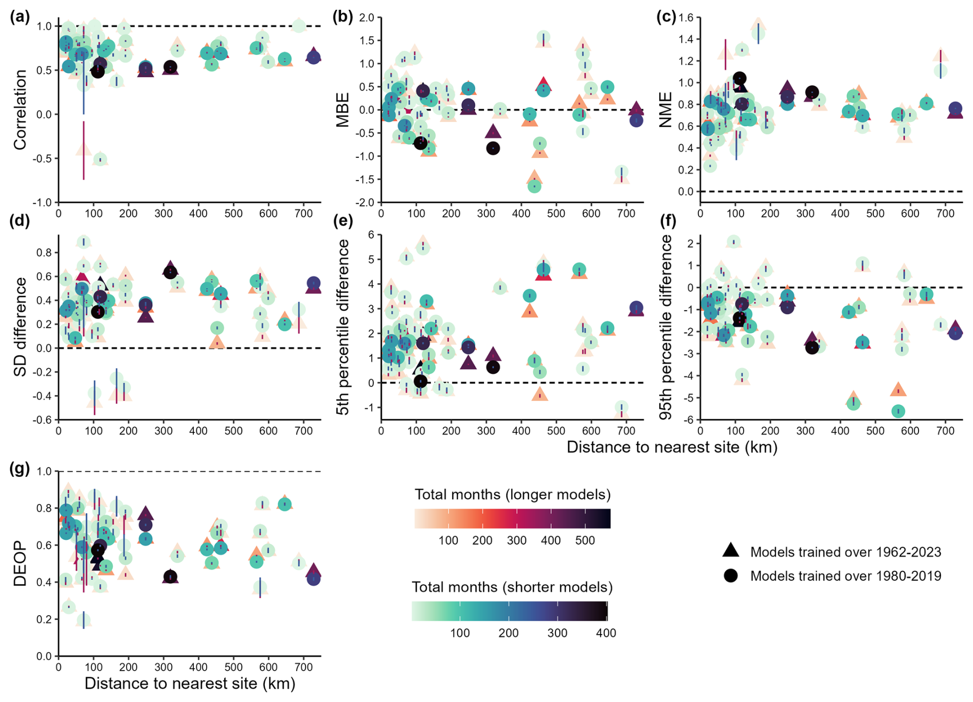
Figure 1 Crossplots summarising a suite of independent metrics describing out-of-sample random forest model skill in predicting spatial δ¹⁸O_P variability. Scores were calculated by removing one site from the training data (the “test site”), training a random forest model using the remaining data, then using that model to predict values for the excluded test site. This process was repeated 50 times for each site, each time initialising the random forest model with a different random seed. Each point shows the skill for a single site. Sites are plotted according to the distance to the nearest site included in the training dataset. Each site has two points on each crossplot: triangles show results for δ¹⁸O_P predicted using the longer models trained over 1962–2023 using the reduced set of predictor variables (without weather objects). Circles show results for δ¹⁸O_P predicted using models trained over 1980–2019 using the full set of predictor variables (including weather objects). Sites are coloured according to record length. The vertical line over each point shows ± one standard deviation in that skill score across the 50 models. In all cases, the dashed black line shows the expected value if the modelled values perfectly matched observations. Panel (a) shows the Pearson correlation coefficient between the observed and modelled monthly δ¹⁸O_P values. Panel (b) shows the Mean Bias Error (MBE). Panel (c) shows the Normalised Mean Error (NME). Panel (d) shows the difference between the Standard Deviation (SD) of the observed and modelled values (following (Abramowitz et al., 2024), a positive value denotes modelled values have lower SD than observations). Panel (e) shows the difference in the 5th percentile of modelled versus observed values (a positive value denotes the 5th percentile of the modelled values has a positive bias relative to observations). Panel (f) shows the difference in the 95th percentile of modelled versus observed values (a negative value denotes the 95th percentile of the modelled values has a negative bias relative to observations). Panel (g) shows the density estimate overlap proportion (DEOP), which summarises the degree of overlap between density estimates calculated for the modelled and observed values (a value of 1 would indicate perfect overlap; 0 would indicate no overlap). See Sect. 2.2.1 or Table S4 in Abramowitz et al. (2024) for skill metric definitions.

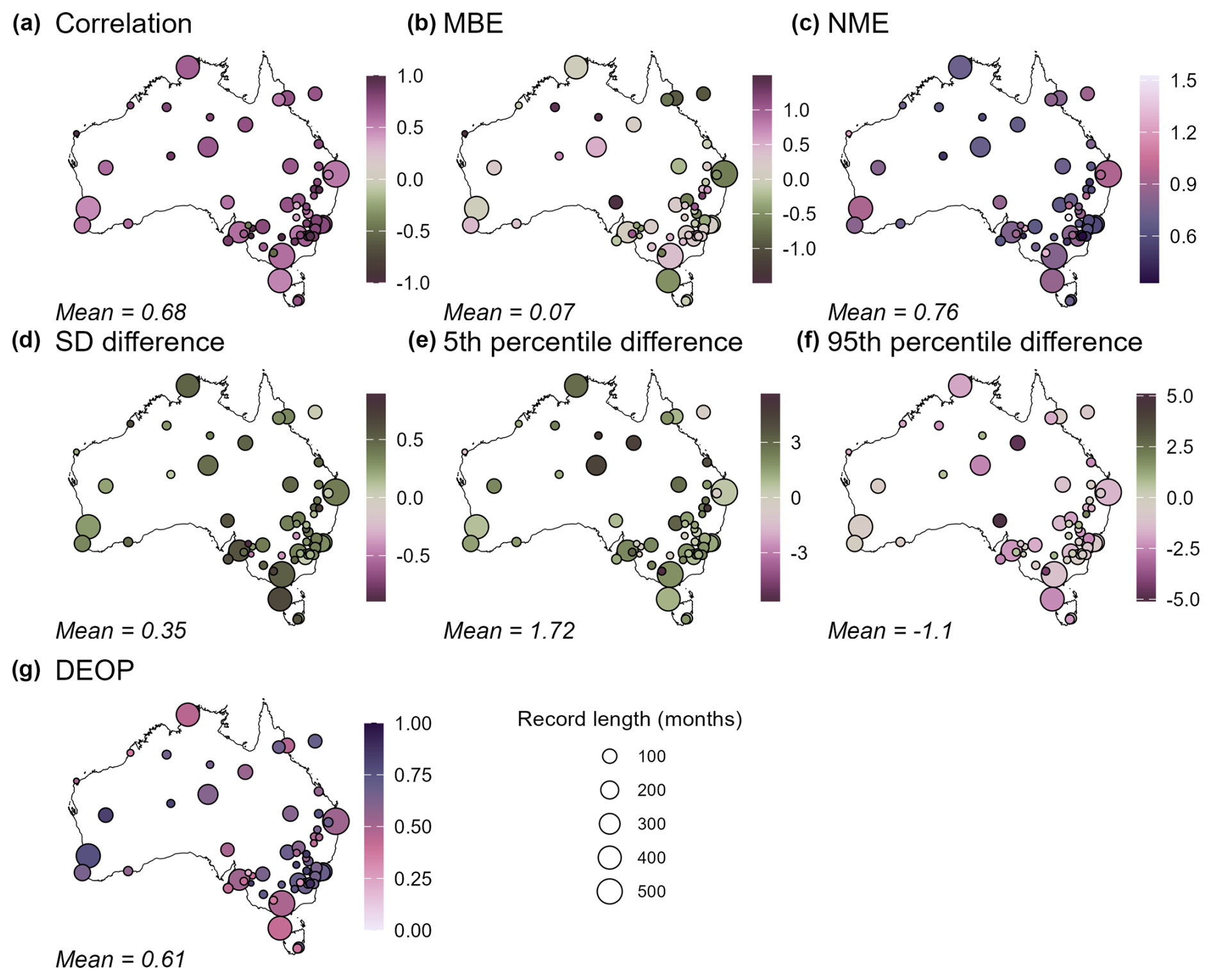
Figure 2 Maps showing average random forest model skill in predicting out-of-sample δ¹⁸O_P variability at the 60 sites across Australia with δ¹⁸O_P observations. Scores were calculated by removing one site from the training data (the “test site”), training a random forest model using the remaining data, then using that model to predict values for the left-out test site. This process was repeated 50 times for each site, each time initialising the random forest model with a different random seed. Points are coloured according to the average skill score from the 50 models, and are sized according to the record length (record lengths range from 2 to 573 months). Values are monthly δ¹⁸O_P predicted using the longer models trained over 1962–2023, using the reduced set of predictor variables (without weather objects). Skill metrics across panels (a)–(g) are all as per Fig. 1. The average skill score across all sites is shown in the lower left corner.

In terms of predictive skill in modelling isotope variability at out-of-sample locations: for all three isotope metrics, there was no relationship between skill and the distance to the nearest site included in the training dataset (Figs. 1, S1–2). This provides confidence that the model predictions for locations with no training data are likely no worse than indicated by the skill tests at the training data locations – noting that on average, for over 98 % of grid cells, > 99 % of predictor values are within the range of the training dataset (Fig. S8).

When predicting values out-of-sample, the random forest models generally under-estimate extreme values at both ends of the distribution. That is, the slope of the linear relationship between observed and modelled values is generally less than 1 (Figs. 5, S9–10). This is the case for both spatial (Figs. 1–2e–f, S1–4e–f) and temporal transitivity (Figs. 3e–f, S5–6e–f), where the modelled 5th percentile values are mostly positively biased, and the modelled 95th percentile values are mostly negatively biased, and standard deviations are mostly lower than in observations. However, the seasonal cycles of δ²H_P, δ¹⁸O_P, and dxs_P are well represented by the random forest models (blue versus grey curves in Figs. 6, S11–12). This is the case even at sites with very few observations (e.g., rows 7–10 of Figs. 6, S11–12).

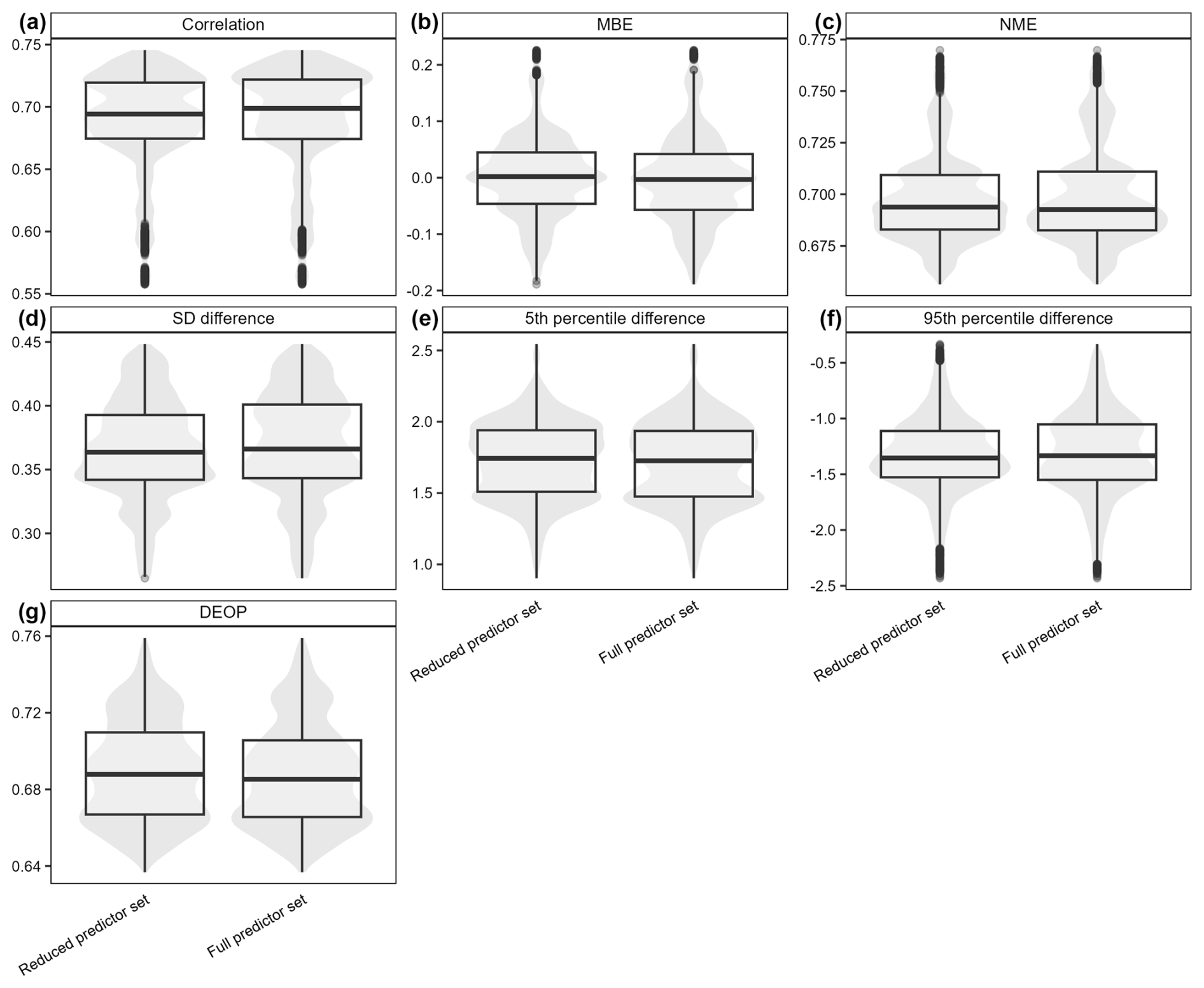
Figure 3 Violin-and-boxplots (“voxplots”) summarising a suite of independent metrics describing model skill in predicting out-of-sample temporal δ¹⁸O_P variability (across all sites). Scores were calculated by removing a random 10 % of all training data, predicting the missing values, then assessing the model's skill in retrieving the held-out data. This process was repeated such that all training data were tested out-of-sample. Additionally, each random forest model was calculated 50 times, each time with a different random seed. These two iterative processes comprise the distributions. In each panel, the left voxplot shows results for monthly δ¹⁸O_P predicted using models trained over 1962–2023, using the reduced set of predictor variables (without weather objects). The right voxplot shows results for monthly δ¹⁸O_P predicted using models trained over 1980–2019, using the full set of predictor variables (including weather objects). Skill metrics across panels (a)–(g) are all as per Fig. 1.

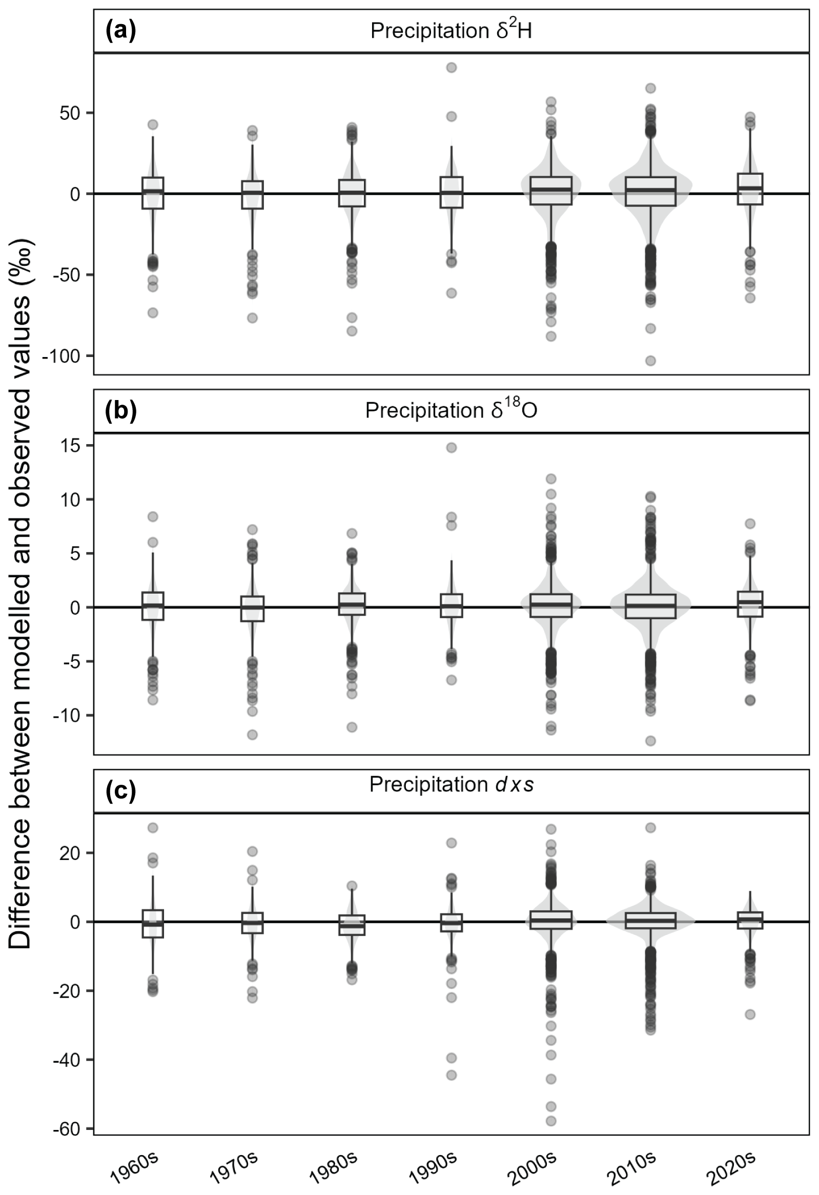
Figure 4 Violin-and-boxplots (“voxplots”) summarising bias in modelled monthly δ²H_P, δ¹⁸O_P, and dxs_P values with respect to observed values at the equivalent months/locations. Each distribution summarises all months at all locations for each decade. Modelled values are from the longer models trained over 1962–2023, using the reduced set of predictor variables (without weather objects), and in all cases are the mean of values predicted by 50 unique random forest models, each initiated with a different random seed. Note that the 1960s and 2020s are incomplete decades (comprising 1962–1969 and 2020–2023, respectively). Voxplot width scales with the number of observations in that decade.

3.1.1 Relative predictability of the three isotope metrics

Predictive skill for δ²H_P and δ¹⁸O_P is similar whilst predictive skill for dxs_P is slightly lower across all metrics. This is the case for out-of-sample skill in both the temporal and spatial domains (Figs. 1–3, 5, S1–6, S9–10), for predictions based on the full training dataset (Figs. 6–7, S11–14), and for the models with the full versus reduced predictor sets. For example, both the mode and shape of site-wise density functions for observed versus modelled δ²H_P and δ¹⁸O_P are similar (Figs. 7, S13, grey versus blue curves). This is particularly the case for sites with over ∼ 50 observations (first four rows in Figs. 7, S13) where there is generally a large overlap between the grey (observations) and blue (random forest models) distributions. Additionally, the random forest models accurately reproduce features such as the left-skewed δ²H_P and δ¹⁸O_P distributions at the tropical sites (Cairns, Willis Island). In comparison, although the mode of the random forest-modelled dxs_P values is generally accurate at sites with over ∼ 50 observations, the distributions generally have excessive kurtosis (Fig. S14).

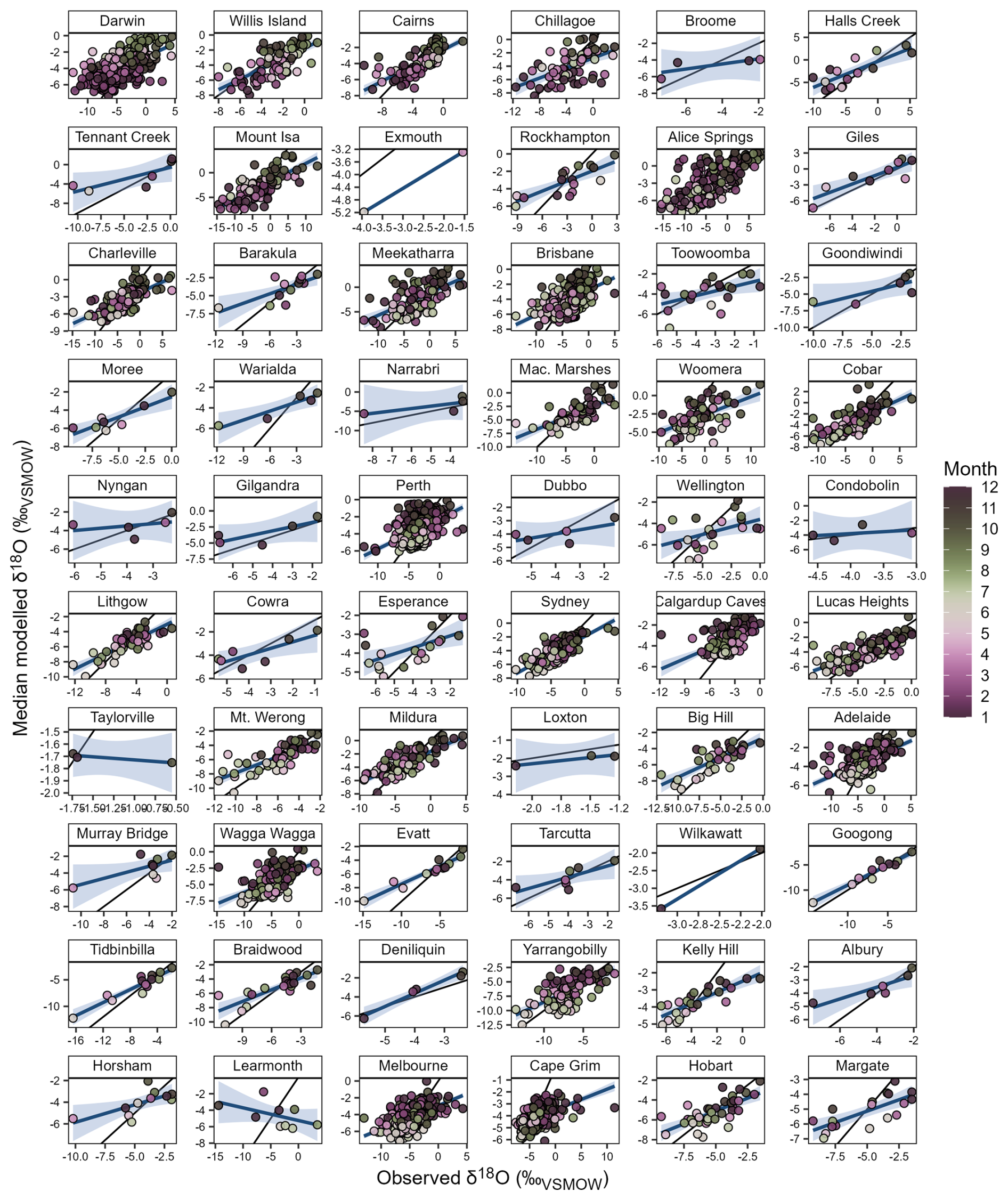
Figure 5 Crossplots comparing modelled and observed monthly δ¹⁸O_P values at the 60 sites across Australia with δ¹⁸O_P observations. For each site, δ¹⁸O_P values were predicted out of sample (i.e., that site's data was removed from the training dataset). Each point shows the mean of values predicted by 50 unique random forest models, each initiated with a different random seed. Sites are arranged by decreasing latitude, with the northern-most site (Darwin) in the top left corner and the southern-most site (Margate) in the bottom right corner. Site details are as per Table S1. In each panel, the thin black line shows the expected relationship if modelled δ¹⁸O_P values exactly matched observations (1:1). The blue line shows the linear relationship between the modelled and observed δ¹⁸O_P values, with the 95 % confidence interval shown in the blue shading. Data points are coloured by month to highlight the seasonal cycle. Values are from the longer models trained over 1962–2023, using the reduced set of predictor variables (without weather objects).

Figure 6 Average seasonal cycle of δ¹⁸O_P at 60 sites across Australia, in observations (grey circles); the random forest models described in this paper (blue diamonds); and the ECHAM6-wiso simulation nudged to the ERA5 reanalysis (see Methods; green squares). Seasonal cycles are calculated from δ¹⁸O_P values in the interval overlapped by all three data sources (1979–2021), and only include months with observations present in all three data sources. In the case of the random forest-predicted δ¹⁸O_P, values are from the longer models trained over 1962–2023, using the reduced set of predictor variables (without weather objects), and show the mean of the 50 models created with unique random seeds. Sites are arranged by decreasing number of observations. Brisbane (top left) has the most observations (n=500); Wilkawatt and Exmouth (bottom right) have the equal fewest observations (n=3).

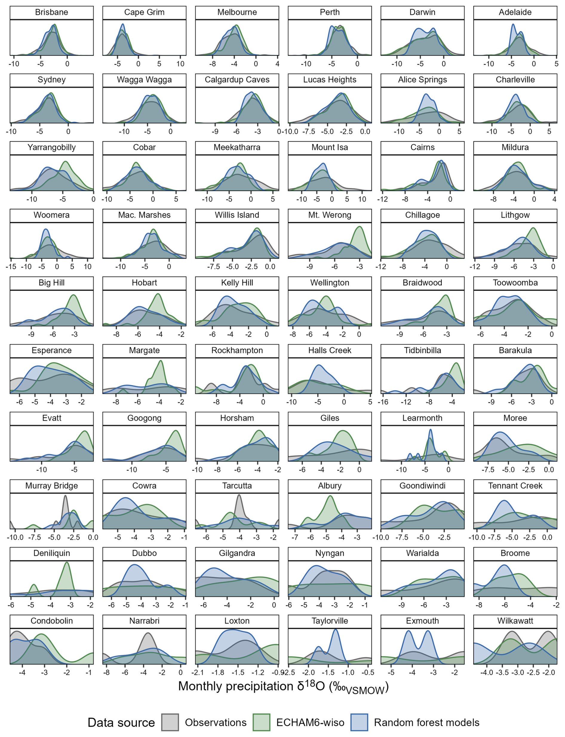
Figure 7 Density plots comparing the distributions of monthly δ¹⁸O_P values at 60 sites across Australia, from observations (grey); the random forest models described in this paper (blue); and the ECHAM6-wiso simulation nudged to the ERA5 reanalysis (see Methods; green). Density curves are calculated from δ¹⁸O_P values in the interval overlapped by all three data sources (1979–2021), and only including months with observations (i.e., curves are constructed with δ¹⁸O_P values from exactly the same months). In the case of the random forest-predicted δ¹⁸O_P, values are from the longer models trained over 1962–2023, using the reduced set of predictor variables (without weather objects), and show the mean of the 50 models created with unique random seeds. Sites are arranged by decreasing number of observations across 1979–2021. Brisbane (top left) has the most observations (n=500); Wilkawatt and Exmouth (bottom right) have the equal fewest observations(n=3).

3.2 Comparison of independently modelled dxs_P with dxs_P calculated from δ²H_P and δ¹⁸O_P

There is minimal difference in long-term dxs_P across the Australian continent as estimated from the independent set of random forest models, compared with long-term mean dxs_P calculated from modelled δ²H_P and δ¹⁸O_P (Fig. 8). Broadly, the independent random forest models (Fig. 8a) predict slightly higher dxs_P across inland western Australia than implied by the δ²H_P and δ¹⁸O_P models (Fig. 8b). The reverse is true for the southern and northern coastline, excepting the far-northern tips of the continent. However, the magnitudes of the difference are small in the long-term annual mean (Fig. 8c).

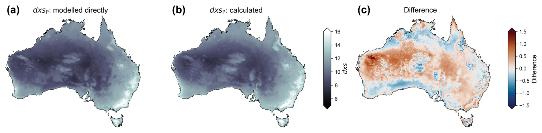
Figure 8 Maps showing the effects of modelling dxs_P across the Australian continent directly versus calculating dxs_P from modelled δ²H and δ¹⁸O. Panel (a) shows long-term annual mean precipitation dxs across the Australian continent, modelled directly as described in Sect. 2.2 (and shown in Fig. 13k). Panel (b) shows long-term annual mean precipitation dxs across calculated from the random forest-modelled δ²H_P and δ¹⁸O_P as follows: dxs_P=δ²H${}_{\mathrm{P}}-\mathrm{8}\times {\mathit{\delta }}^{\mathrm{18}}$O_P. Panel (c) shows the difference between dxs_P as estimated by the two approaches; the dxs_P values implied by the separate δ²H_P and δ¹⁸O_P models subtracted from the directly-modelled dxs_P values.

3.3 Key predictors of δ²H_P, δ¹⁸O_P, and dxs_P spatio-temporal variability

For the final models (incorporating all training data), precipitation amount and precipitation intensity were the most important predictors of δ²H_P and δ¹⁸O_P spatio-temporal variability (Fig. 9). Relative humidity, surface temperature, the ratio of convective to total precipitation, and the seasonal cycle were also important. For dxs_P, surface temperature and mean sea level pressure were the most important predictors, followed by precipitation amount and relative humidity.

In the shorter models including the weather object data, the weather objects (shown in lavender on Fig. 9) were generally of middling importance, with precipitation delivered by potential vorticity streamers the most important weather object for spatio-temporal variability in all three isotope metrics. Remote drivers (e.g., ENSO, SAM, shown in green) tended to be less important across all isotope metrics. Of the remote drivers, the ΔSLP and Niño 3.4 indices for tropical Pacific variability were the most important. The fraction of precipitation delivered as snow was the least important predictor of spatio-temporal variability in all isotope metrics – likely because it is only relevant for a very small geographical region. Nevertheless, all predictors contributed meaningfully to the final models. Predictor importance was robust to the inherent randomness of the models, with minimal differences between the models produced with the 50 unique seeds.

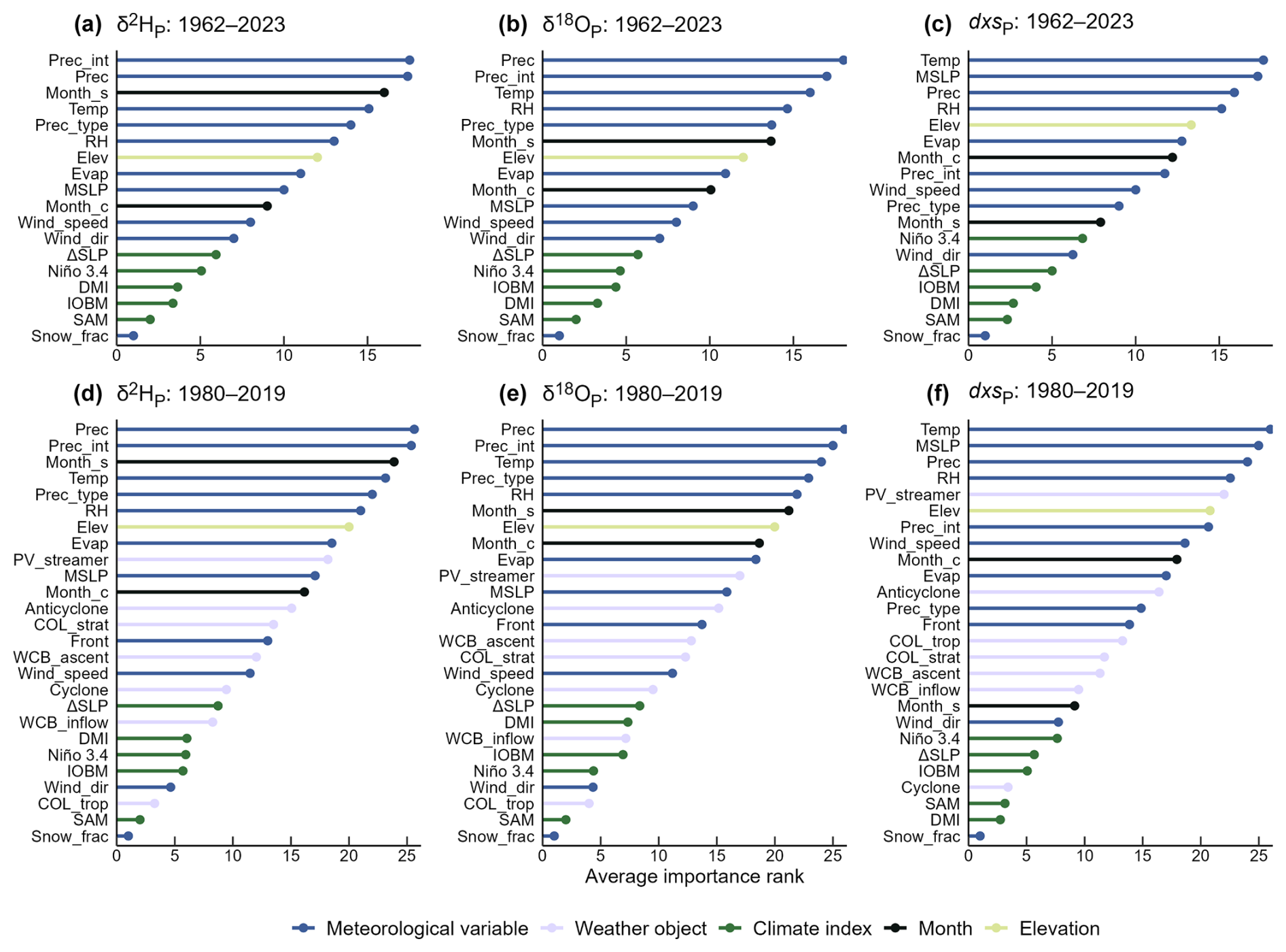
Figure 9 Average importance rank of each predictor variable with respect to the random forest models' predictive performance, calculated using the “permutation” method. The panels show the overall rank of each variable's relative importance in predicting spatio-temporal precipitation isotopic variability across the Australian continent. Ranks are the average for that variable across 50 random forest models, each created with a different random seed. The least important variable for a predictor model receives a rank of 1; the most important variable receives a rank equal to the number of variables included. So, the most important variables for the model are shown at the top of each panel; the least important at the bottom. Predictors are coloured according to the variable type: blue for meteorological variables, lavender for weather objects, forest green for climate indices (representing remote dynamical drivers), black for month of the year, and lime green for elevation. Panel (a) shows results for the δ²H_P models trained over 1962–2023, using the reduced set of predictor variables (without weather objects). Panel (b) is as per panel (a) but for δ¹⁸O_P. Panel (c) is as per panel (a) but for dxs_P. Panels (d)–(f) are as per panels (a)–(c) but for the models trained over 1980–2019, using the full set of predictor variables (including weather objects). Variable names and descriptions are as per Table S2.

3.3.1 Predictor importance for individual sites

Predictor importance for temporal variability in δ²H_P, δ¹⁸O_P, and dxs_P varied by site (Fig. 10). For δ²H_P and δ¹⁸O_P: precipitation amount, precipitation intensity, relative humidity, and the seasonal cycle were prevalent in the top five most important predictors across sites, but other variables – including those less important for continental spatio-temporal δ²H_P and δ¹⁸O_P variability – also scored highly. These include the ratio of convective to total precipitation and local evaporation; weather objects also regularly featured in the five most highly-ranked predictors.

Relative to δ²H_P and δ¹⁸O_P, there was more inter-site variability in dxs_P predictor importance (Fig. 10 third column). Both surface temperature and precipitation delivered by potential vorticity streamers appeared the most frequently in the five most highly-ranked predictors across the five sites. Weather objects (shown in lavender) tended to be ranked more highly than for δ²H_P and δ¹⁸O_P, with local precipitation amount and intensity generally less important.

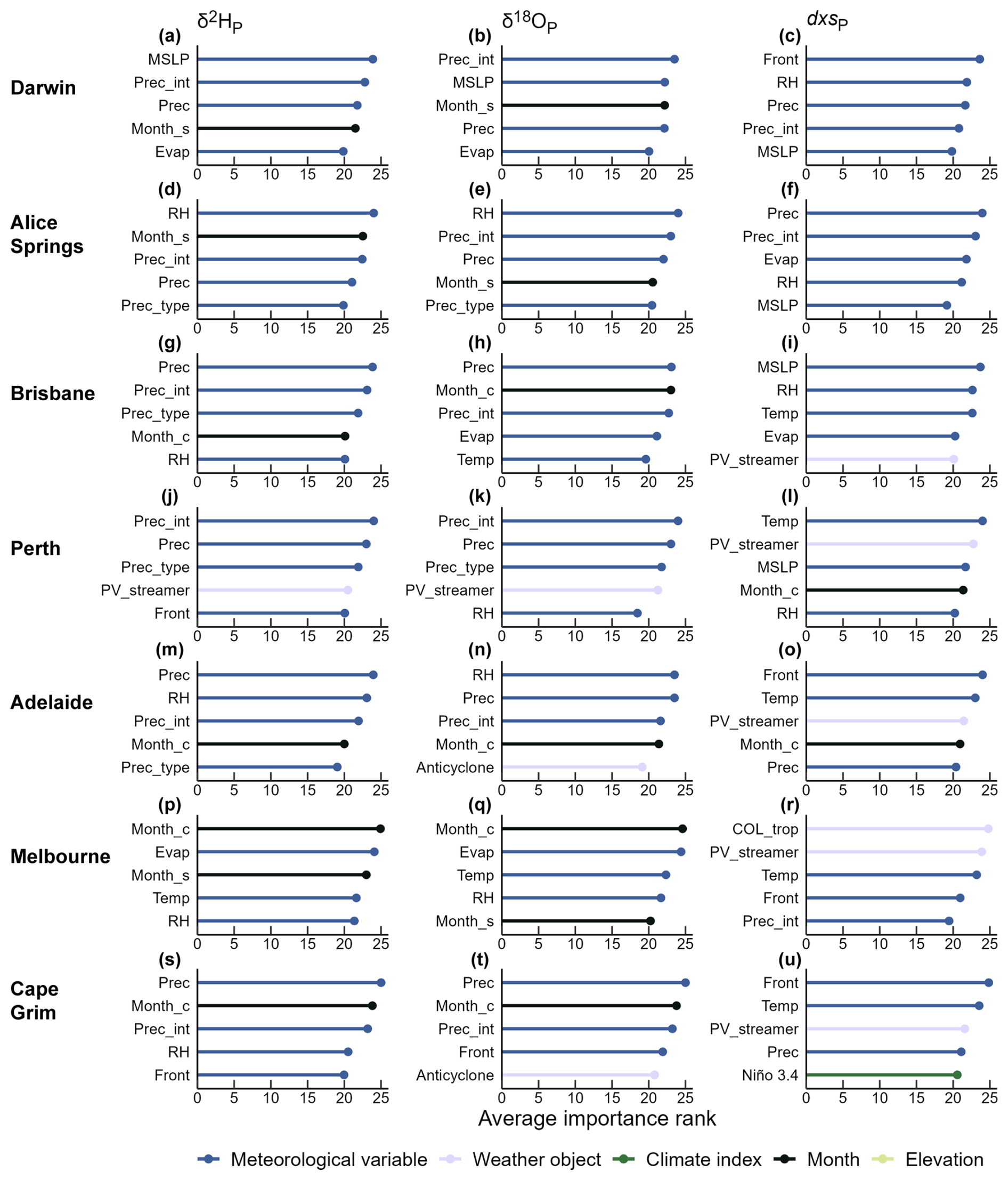
Figure 10 Average importance rank of each predictor variable with respect to the random forest models' predictive performance, calculated using the “permutation” method. The panels show the overall rank of each variable's relative importance in predicting temporal precipitation isotopic variability at the seven longest precipitation isotopic monitoring stations in Australia. Site details are as per Table S1. Sites are arranged in order of descending latitude from top to bottom. Ranks are as per Fig. 9, with the most important variable receiving the highest rank, and less important variables receiving lower ranks. As per Fig. 9, predictors are coloured according to the variable type; variable names and descriptions are as per Table S2. Here only showing the five most important predictor variables at each site. The first column shows results for δ²H_P predicted at the seven sites, with models trained over 1980–2019, using the full set of predictor variables (including weather objects). Second column is as per the first column but for δ¹⁸O_P. Third column is as the first column but for dxs_P.

3.4 Spatio-temporal variability in precipitation stable isotopes over the Australian continent

The spatio-temporally complete modelled dataset shows clear interannual variability in all three isotope metrics (Figs. 11–12, S15–16). For one example, the unprecedentedly extreme 2017–2019 eastern Australian “Tinderbox” drought (Devanand et al., 2024; Falster et al., 2024) is associated with distinct isotopic anomalies in the annual mean (see also Fig. S17). This is particularly the case for dxs_P, where negative dxs_P values associated with the final year of the drought are the most extreme of any in the past 20 years (Figs. S16–17).

In terms of the total range of values spanned at any one location (i.e., the maximum value occurring at a location minus the minimum value occurring at that location, across 1962–2023), monthly precipitation isotopic ranges span 30.1–114.3 ‰, 4.1–17.4 ‰, and 5.7–30.9 ‰ for δ²H, δ¹⁸O, and dxs, respectively (Fig. 12a–c). Annual-mean site-wise total ranges span 5–61.7 ‰, 0.5–9.4 ‰, and 0.8–12.7 ‰ for δ²H, δ¹⁸O, and dxs, respectively (Fig. 12d–f).

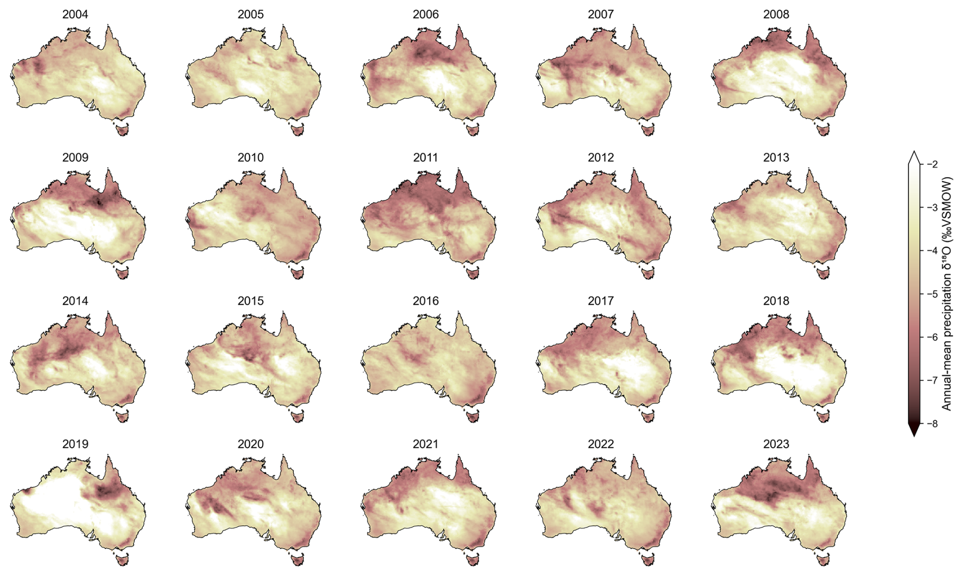
Figure 11 Precipitation amount-weighted annual mean δ¹⁸O_P values across Australia for the 20 most recent years of the random forest models trained over 1962–2023, using the reduced set of predictor variables (without weather objects).

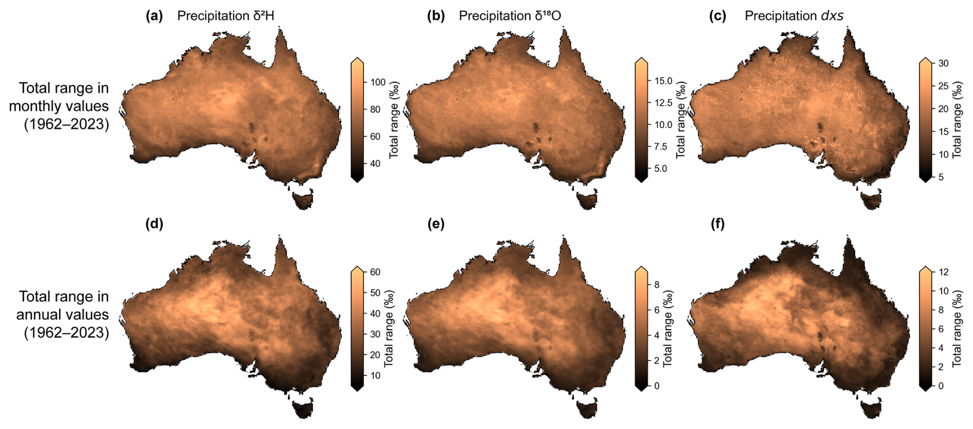
Figure 12 Maps showing the total range in precipitation isotopic values over the 1962–2023 period. Maps show the total inter-month (top row) and inter-annual (bottom row) range in δ²H_P (first column), δ¹⁸O_P (second column) and dxs_P (third column) values at all locations across the Australian continent. That is, at each location the maps shows the difference between the most positive value occurring in the 1962–2023 period and the most negative value occurring in that period. Ranges calculated using the random forest models trained over 1962–2023, using the reduced set of predictor variables (without weather objects). Annual values are precipitation amount-weighted annual means.

3.5 Comparison with precipitation isotopic estimates from other sources

3.5.1 Monthly variability

In terms of both the seasonal cycle (Figs. 6, S11–12, grey versus blue and green curves) and the overall distribution of values (Figs. 7, S13–14), the random forest models generally outperform the physically-based ECHAM6-wiso estimates of δ²H_P, δ¹⁸O_P, and dxs_P for the equivalent months. For example, the site-wise seasonal cycles of δ²H_P and δ¹⁸O_P in ECHAM6-wiso (green curves in Figs. 6, S11) are generally damped (e.g., Yarrangobilly, Mt. Werong), offset (e.g., Cape Grim, Macquarie Marshes), or both (e.g., Melbourne) relative to both observations and the random forest models. The random forest models perform particularly well compared with ECHAM6-wiso in retrieving the seasonal cycle of dxs_P, where the random forest models generally capture both the magnitude and timing of the seasonality, but estimates from ECHAM6-wiso generally have either a larger overall bias (e.g., Margaret River, Lucas Heights) and/or bias in the seasonal cycle magnitude (e.g., Brisbane, Sydney) (Fig. S12).

Differences in skill between the two models are less distinct in predicting the overall distribution of δ²H_P and δ¹⁸O_P values (Figs. 7, S13) – both the random forest and general circulation models perform well. Whilst the distributions of random forest-predicted values are generally closer to observations than those predicted by ECHAM6-wiso, there are sites where ECHAM6-wiso out-performs the random forest models (e.g., Adelaide, Alice Springs). There are also instances where estimates from the two models are similar but both diverge from observations (e.g., Lucas Heights, Mt. Isa). The dxs_P estimates from ECHAM6-wiso lack the positive kurtosis of the random forest estimates (Fig. S14). However, the ECHAM6-wiso estimates have a negative dxs_P bias at most sites; this negative bias is not present in the random forest estimates.

3.5.2 Long-term mean precipitation isoscapes

In terms of the long-term mean annual-mean δ²H_P and δ¹⁸O_P across the Australian continent (“time-mean isoscapes”; Fig. 13), there are some similarities between estimates from the random forest models, the physical ECHAM6-wiso model (Cauquoin and Werner, 2021), and linear regressions using geographic variables (Hollins et al., 2018). Common features include: relatively negative values over the Australian Alps, relatively positive values in south-central continental Australia, and a trend to more negative values northward and westward (Fig. 13a–j). The random forest and linear regression time-mean isoscapes also predict relatively negative δ²H_P and δ¹⁸O_P values over the Tasmanian Alps. The ECHAM6-wiso and linear regression time-mean isoscapes predict large areas of very negative δ²H_P and δ¹⁸O_P across northern Australia; these are not so strongly present in the random forest isoscape.

The three dxs_P time-mean isoscapes are quite different (Fig. 13k–o). Overall, there are more similarities between the two statistically-derived isoscapes where dxs_P was modelled directly (random forests and linear regressions) than the physically-based isoscape (ECHAM6-wiso) where dxs_P was calculated from δ²H_P and δ¹⁸O_P. For example, the random forest and linear regression time-mean isoscapes predict relatively positive values over higher-elevation areas (Australian Alps, Tasmanian Alps, MacDonnell Ranges). These features are not present in the ECHAM6-wiso dxs_P time-mean isoscape which relies on accurate modelling of the relative variability in δ²H_P and δ¹⁸O_P.

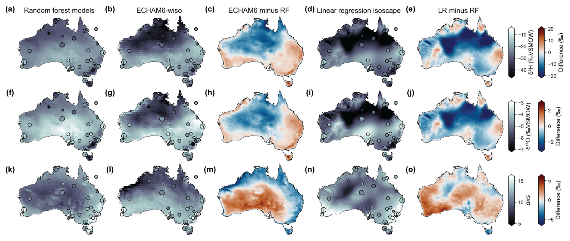
Figure 13 Long-term annual mean precipitation isotopic variability across the Australian continent (“time-mean isoscapes”). Panel (a) shows long-term (1962–2023) annual-mean precipitation amount-weighted δ²H_P as calculated from the random forest models described in this paper (showing the mean of the 50 models created with unique random seeds). Panel (b) shows long-term (1979–2021) annual-mean precipitation amount-weighted δ²H_P as simulated by ECHAM6-wiso nudged to ERA5 (Cauquoin and Werner, 2021). Panel (c) shows the difference between climatological δ²H_P from ECHAM6-wiso and the random forest models (i.e., panel b minus panel a). Panel (d) shows long-term (1962–2014) annual-mean precipitation amount-weighted δ²H_P as estimated by linear regression using geographical variables (Hollins et al., 2018). Panel (e) shows the difference between climatological δ²H_P from the linear regression and the random forest models (i.e., panel d minus panel a). Panels (f)–(j) are as per panels (a)–(e) but for δ¹⁸O_P. Panels (k)–(o) are as per panels (a)–(e) but for dxs_P. Note that the isoscapes from Hollins et al. (2018) were calculated using data spanning 1962–2014, which exceeds the total coverage of the ECHAM6-wiso simulation. As we could not average across matching time periods for all three data sources, we show annual means across each dataset's entire coverage interval to provide the most representative long-term isoscapes. Points show the long-term annual mean precipitation isotopic values at each site with 2 or more years of observations (see Sect. 2.4 for details). Point sizes scale log-linearly with record length (in years).

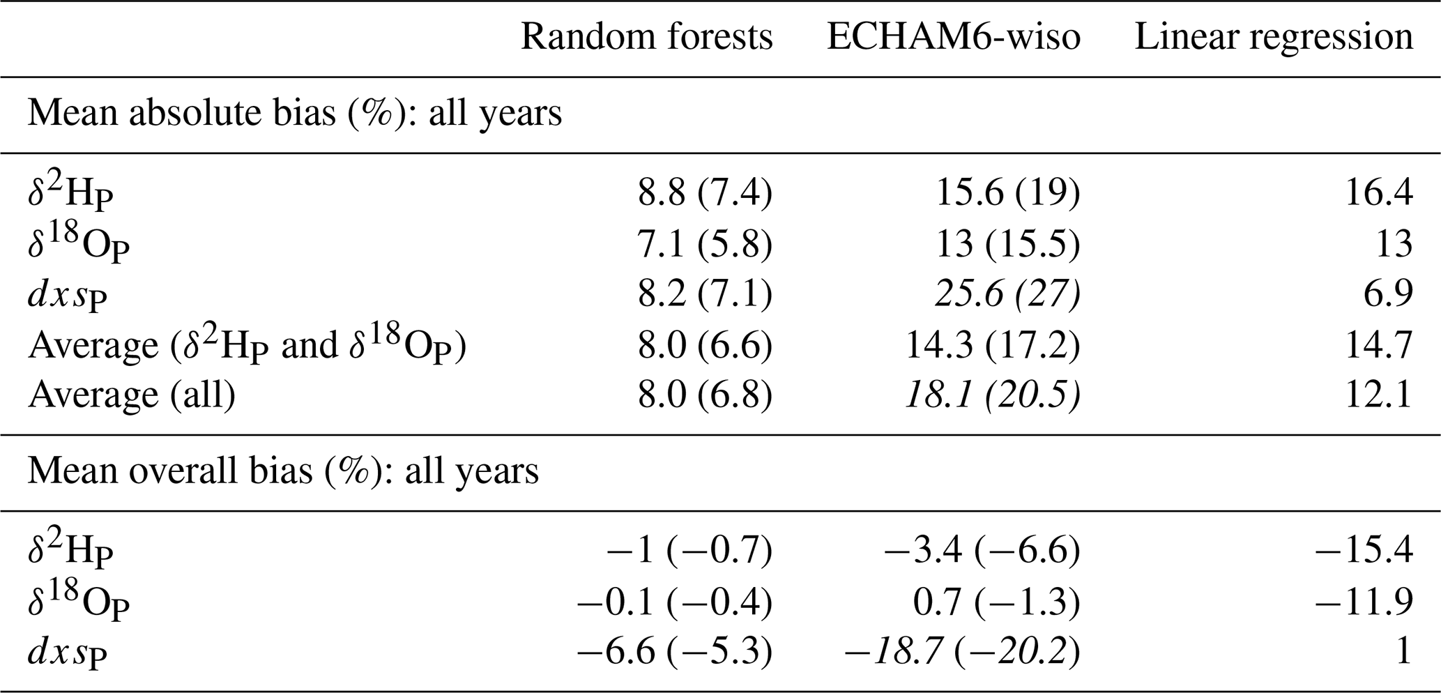
The random forest δ²H_P and δ¹⁸O_P time-mean isoscapes are the most similar to long-term mean annual-mean observations; the linear regression-based isoscape has slightly lower absolute dxs_P bias at the sites/years with observations (mean absolute bias in Table 1). In the random forest δ²H_P and δ¹⁸O_P time-mean isoscapes, values tend to be positively biased in central to north-western Australia, and negatively biased in eastern Australia (Figs. S18–19). The reverse is broadly true for the ECHAM6-wiso time-mean isoscape; most sites have a negative bias in the linear regression isoscape (Fig. S18, mean overall bias in Table 1). The random forest dxs_P time-mean isoscape has a negative bias at most sites (Figs. S18g, S19f, mean overall bias in Table 1). Overall, the random forest models' absolute biases are similar across the three isotope metrics (Table 1). The ECHAM6-wiso dxs_P time-mean isoscape has much larger mean absolute bias than the ECHAM6-wiso δ²H_P and δ¹⁸O_P isoscapes; the linear regression dxs_P isoscape has much smaller mean absolute bias than the linear regression δ²H_P and δ¹⁸O_P isoscapes (Table 1). When biases are calculated using only model values in years with observations (as opposed to the full long-term mean), the random forest models' absolute biases are uniformly lower; the ECHAM6-wiso biases are higher (Fig. S19, Table 1). Nevertheless, the values are similar to those calculated using all model years, suggesting that these bias estimates provide a reasonable approximation of skill across the three time-mean isoscapes.

Table 1 Modelled isoscape δ²H_P, δ¹⁸O_P, and dxs_P bias with respect to observed long-term means. Only including sites with five or more years of observations. The values state the average bias across all sites (shown in Figs. 13, S18). All bias estimates are shown as a percentage of the total range of variability in that particular isotope metric (δ²H_P, δ¹⁸O_P, or dxs_P). Values in parentheses were calculated using the subset of values present in both the random forest and ECHAM6-wiso datasets, to facilitate direct comparison between the two (shown in Fig. S19). Rows in the top half of the table show the absolute bias values; rows in the bottom half of the table show the overall bias (i.e., highlighting the average direction of each product's bias). Note that dxs_P was modelled directly in the random forest and linear regression models. For ECHAM6-wiso, dxs_P was calculated from the simulated δ²H_P and δ¹⁸O_P and the bias values are shown in italics. To facilitate fair comparison, we show the average absolute bias for only δ²H_P and δ¹⁸O_P (estimated directly in all three products) as well as the average absolute bias across the three isotope metrics.

4 Discussion

Our new spatially and temporally continuous estimates of monthly δ²H_P, δ¹⁸O_P, and dxs_P reveal strong variability across the Australian continent, both in space (Fig. 13) and through time (Figs. 11–12, S15–16). Rainfall-related climate extremes (e.g., the 2017–2019 Tinderbox Drought; Fig. S17) are reflected in distinct isotopic anomalies, suggesting that dynamical atmospheric processes associated with extreme climate events could be further interrogated using precipitation isotopic data. Importantly, we show that even at individual locations, both monthly and interannual variability in the isotopic composition of precipitation is high (Fig. 12). This has implications for water isotope-based provenance studies, which have often relied on temporally invariant isoscapes for isotopic fingerprinting (e.g., Fig. 12 compared with Fig. 13).

Comprehensive skill testing suggests that random forest modelling is a robust method for reliably estimating water isotope variability across the Australian continent in places/times where direct observations are not available. This may include both sites lacking observations, and times at current or previous monitoring stations where data were not collected. Random forest models may be particularly useful for the latter, given their relatively high skill in filling time gaps (Figs. 3, S5–6).

4.1 Reasons for mismatch between modelled and observed values

As is common for any predictive model of physical climate variables (e.g., Hill et al., 2025; Nelson et al., 2021), the random forest models tend to under-estimate extreme values in all three isotope metrics (Figs. 5, S9–10). This may be due to several factors. First, the most extreme monthly δ²H_P, δ¹⁸O_P, and dxs_P values may be driven by a small number of extreme precipitation events (e.g., Griffiths et al., 2022; Munksgaard et al., 2012), which ERA5 underestimates compared with precipitation events closer to the mean (Lavers et al., 2022). Second, we may have missed predictor variables specifically relevant for the most extreme negative or positive δ²H_P, δ¹⁸O_P, and dxs_P values that have also not been previously identified in the literature or are not practical for inclusion in random forest models. Third, the mismatch in the extremes may be due to observational error, and therefore not well simulated by the random forest models that are mostly trained on data closer to the median. For example, during low precipitation months, high δ²H_P and δ¹⁸O_P and low dxs_P values may result from evaporation during sample collection (discussed in Sect. 4.2 in more detail). Fourth, random forest modelling is an ensemble method where each prediction is the average of predictions from all trees. This approach enhances robustness to biases by reducing the influence of any single tree's error. However, it also dampens extremes due to the averaging process, limiting the models' ability to capture outliers.

Regarding the lower skill in simulating dxs_P relative to δ²H_P and δ¹⁸O_P: compared with δ²H_P and δ¹⁸O_P, dxs_P variability is strongly driven by ambient conditions at the precipitation source (Pfahl and Sodemann, 2014). Moisture source conditions are not well captured in our models, which by necessity rely on largely site-level predictors. The shorter models – incorporating the weather object data – predicted dxs_P more skillfully than the longer models without the weather objects. Further, the skill increase resulting from inclusion of the weather objects was larger for dxs_P than for δ²H_P and δ¹⁸O_P, suggesting that the moisture source and transport information inherent in the weather objects is particularly important for dxs_P. Nevertheless, these proxies for the moisture source location and conditions were evidently insufficient for fully capturing spatio-temporal dxs_P variability. Future work could attempt to incorporate information about moisture source and transport path via moisture parcel back-trajectory analysis (e.g., Munksgaard et al., 2012; Stein et al., 2015), although this would be computationally expensive as calculations would need to be performed for all precipitation events in all months, at all grid cells (in this case, 744 months for > 8 000 000 grid cells).

4.2 Comparison with linear regression isoscape and isotope-enabled model

In terms of long-term mean annual-mean δ²H_P and δ¹⁸O_P, the random forest models have lower absolute bias than linear regression-based isoscapes using only geographical predictors (Hollins et al., 2018) – despite the random forest models being calculated at lower spatial resolution (Fig. S18, Table 1). This demonstrates the importance of meteorological and dynamical variables for precipitation isotope variability across the Australian continent – and that the impact of that variability on precipitation isotopes is not solely controlled by geography.

One of the major advances of our new random forest models from the linear regression-based isoscape is the addition of the time dimension. Information about spatio-temporal precipitation isotope variability was previously available from isotope-enabled GCMs, including the state-of-the-art nudged isotope-enabled ECHAM6-wiso model. Like the random forest models, ECHAM6-wiso accurately simulates the seasonal cycle and overall distribution of δ²H_P, δ¹⁸O_P, and dxs_P values at most sites (Figs. 6–7, S11–14). However, ECHAM6-wiso predictions of long-term mean δ²H_P, δ¹⁸O_P, and dxs_P are less accurate in high-elevation regions (Figs. 13, S19). This lower accuracy at high-elevation sites is likely due to the lower spatial resolution of ECHAM6-wiso (0.9°) compared with the random forests (0.25°), affecting the model topography (Cauquoin and Werner, 2021). High-elevation regions such as the Australian and Tasmanian alps form the headwaters for catchments important for both domestic water supply and generation of hydro-electric power (Donohue et al., 2011). The random forests' relatively high skill in modelling high-elevation precipitation isotopic variability will therefore be particularly useful in understanding surface water and groundwater movements in catchments critical for Australia's water security.

Inland and western Australia are poorly sampled by the observational network, making our new estimates particularly useful in these areas. Broadly, the random forest isoscapes predict higher inland climatological δ²H_P and δ¹⁸O_P values than ECHAM6-wiso; the reverse is true for dxs_P (Fig. 13, fourth and fifth columns). It is difficult to say which is more accurate – Fig. S18 shows that the random forests tend to overestimate inland δ²H_P and δ¹⁸O_P values with respect to observations, but ECHAM6-wiso tends to underestimate them. These differences may be influenced by bias in the observational training data. Inland Australia is climatologically hot and dry, and is sparsely populated. Because of this sparse population, in many cases precipitation samples for isotopic analysis are collected via composite samplers rather than daily rainfall collection, despite the dry climate. Composite samplers tend to be associated with isotopic bias in low-rainfall months, resulting in a positive (but not systematic) bias in δ²H_P and δ¹⁸O_P values. Accordingly, ECHAM6-wiso – which directly simulates processes important for inland precipitation δ²H $/$ δ¹⁸O $/$ dxs, such as sub-cloud evaporation (Crawford et al., 2017) – underestimates inland precipitation δ²H $/$ δ¹⁸O with respect to observations, but may in fact be closer to the true values. Nevertheless, as shown in Table 1 (and apparent visually from Fig. S18 for the inland sites), the overall magnitude of the (apparent) bias in the random forest isoscapes is less than that of ECHAM6-wiso and this is essentially impossible to test further without new observational data.

4.3 Drivers of precipitation isotopic variability across the Australian continent

Australia's precipitation is highly variable both spatially and temporally, with large gradients in precipitation amount and seasonality across the continent, and large variations from year to year (Nicholls et al., 1997). Our models reveal that this spatio-temporal heterogeneity in Australian precipitation and its intensity is closely linked to spatio-temporal heterogeneity in the isotopic composition of that precipitation (Fig. 9). However, relative predictor importance for monthly δ²H_P, δ¹⁸O_P, and dxs_P variability varies spatially (Fig. 10) – reflecting the large spatial variability in the drivers, sources, and seasonality of Australian precipitation. For example, tropical northern Australia receives most of its rainfall in the austral summer, with rain generally delivered by monsoon troughs and tropical cyclones (Sharmila and Hendon, 2020; Suppiah, 1992). Moisture in the monsoon season mostly originates from the proximal seas north of Australia, with up to ∼ 11 % local recycled precipitation (Holgate et al., 2020). In comparison, much of southern Australia has winter-dominated precipitation, with moisture generally delivered by extratropical cyclones, fronts, and thunderstorms, and minimal precipitation recycling (Holgate et al., 2020; Pepler et al., 2020, 2021). Inland Australia is mostly arid, with highly variable precipitation (Van Etten, 2009), delivered by a wide range of weather systems (Acworth et al., 2016), and with moisture sourced from oceans all around Australia as well as terrestrial recycling (Acworth et al., 2024; Holgate et al., 2020). South of the tropics, moisture sources to the Australian continent vary widely, with the Coral and Tasman seas supplying much of the south-eastern to eastern coasts, and the proximal Indian and Southern oceans supplying south-western Australia (Holgate et al., 2020). The timing and source of precipitation over the Australian continent is influenced by both local weather systems and remote drivers (Risbey et al., 2009) – including ENSO (McBride and Nicholls, 1983), the IOD (Ummenhofer et al., 2009), and the SAM (Hendon et al., 2007).

Accordingly: at Darwin in tropical northern Australia, mean sea level pressure, rainfall amount, and rainfall intensity are in the top five most important predictors of variability in all three isotope metrics (Fig. 10 top row). This is likely linked to the monsoon troughs typically associated with the intense rainfall delivered during “active” phases of the austral summer monsoon season – and which are associated with moisture that generally comes from the same source region and follows the same trajectory (Berry and Reeder, 2016). Rain delivered during “inactive” phases of the monsoon is typically not associated with a monsoon trough, and results from a different range of circulation and moisture flux regimes (Godfred-Spenning and Reason, 2002). In contrast, at Cape Grim in south-eastern Australia (Fig. 10 bottom row): whilst precipitation amount and intensity are important for precipitation isotopic variability, the particular weather systems delivering that precipitation – including fronts, anticyclones, and potential vorticity streamers – are also important. This is likely due in part to these systems bringing precipitation along different trajectories from different ocean sources.

4.4 Applications

Our analyses reveal distinct spatial and temporal variability in δ²H_P, δ¹⁸O_P, and dxs_P across the Australian continent. This isotopic heterogeneity – combined with the random forest models' unprecedented out-of-sample skill, high spatial resolution, and monthly temporal resolution over a span of 62 years – provides a strong foundation for future Australia-focussed hydrological, ecological, and archaeological research (e.g., Adams et al., 2022, 2023; Bunney et al., 2023; Gibson et al., 2008; Keegan-Treloar et al., 2024; McInerney et al., 2023; Theden-Ringl et al., 2011), as well as food provenancing (e.g., Anh et al., 2022; Simpkins et al., 1999) and forensic investigations (e.g., Jones et al., 2016; Smith et al., 2022). Further, site-level research previously restricted to using precipitation isotopic data from the nearest GNIP station – often over > 100 km away (e.g., Banks et al., 2021; Buzacott et al., 2020; Zhou et al., 2022) – can now incorporate site-specific estimates from our spatio-temporally continuous random forest model outputs.

The new δ²H_P, δ¹⁸O_P, and dxs_P maps provide an unprecedented opportunity for quantifying the particular hydroclimatic signal/s preserved in water isotope proxy records (e.g., better defining modern isotope-climate relationships), which can then be reconstructed over preceding centuries to millennia. This will be especially valuable for input to proxy system models (Dee et al., 2015; Evans et al., 2013), which explicitly resolve the range of environmental processes by which a precipitation isotopic signal is encoded in a particular palaeoclimate archive (e.g., tree wood, Roden et al., 2000, lake sediment, Dee et al., 2018, cave carbonate, Hu et al., 2021). Proxy system models can provide detailed insights into the drivers of temporal variability in a water isotope proxy record – and ultimately more accurate palaeoclimate reconstructions – but generally require estimates of precipitation isotopic variability as inputs.

5 Conclusions

We developed a dataset of monthly δ²H_P, δ¹⁸O_P, and dxs_P values at 0.25° spatial resolution from 1962–2023 over the entire Australian continent, using a random forest modelling approach. The dataset provides unprecedented insights into precipitation isotope variability in both space and time, as well as the drivers of that variability. The precipitation isotope data are predicted using a freely available suite of meteorological, geographical, and dynamical variables. Additional models spanning 1980–2019 include a set of “weather object” data, but the predictive skill increase from addition of these additional predictors is mainly restricted to dxs_P. Our preliminary analyses reveal distinct spatial and temporal variability in δ²H_P, δ¹⁸O_P, and dxs_P values across the Australian continent, with applications in many fields. Future work will focus on quantifying the nature and drivers of spatio-temporal variability in Australian precipitation isotope variability.

We show that random forest modelling provides an accurate and inexpensive means of estimating missing δ²H_P, δ¹⁸O_P, and dxs_P values both in space and through time. Prediction errors relative to observations are lower than existing predictive tools. For an area the size of the Australian continent – and using a carefully-selected suite of predictor variables – random forest models can be built and tested on a personal computer using open-source software. Our methods therefore provide an accessible framework for predicting water isotope values in other locations with sufficient observational data density.