Evaluation of a socio-hydrological water resource model for drought management in groundwater-rich areas

Groundwater is a drought resilient source of water supply for many water users globally. Managing these highly-used groundwater stores is complicated by the episodic nature of droughts and by our limited understanding of water systems’ response to extreme events. Models are useful tools to simulate a range of prepared drought interventions, however, we need to ensure robust representation of surface water and groundwater storage, users of both resources, and associated management interventions for drought resilience. A robust modelling approach is therefore essential for decision-making in groundwater management.

In this study, we present a Socio-Hydrological Water Resource (SHOWER) model for drought management in groundwater-rich regions. We evaluate SHOWER using a response-based and a data-based model evaluation in Great Britain which considers the modelling uncertainty, dynamic impact of management and modelling setups available. In the response-based evaluation, we first examined the model consistency with our understanding of the system functioning and evaluated the influence of modelled management scenarios in normal and droughts conditions on discharge and groundwater levels. Secondly, in the data-based evaluation we tested the accuracy of heavily influenced discharge and groundwater level simulations in three catchments representative of typical hydrogeological conditions and water management practices in Great Britain. Results from the response-based method show consistent simulations for all model setups. We identified which parameters were influential to model output at which times. Integrated water management interventions have significant impact on flows and groundwater beyond parameter uncertainty and show leverage to reduce droughts by minimising shortages in water demand. The data-based analysis shows that calibration can be focused on either source-specific or combined model outputs using a “best overall” calibration approach that captures groundwater levels and low flows. The source-specific calibrations result in the highest and narrowest KGE ranges for discharge and groundwater (KGE: 0.75–0.84 and 0.62–0.95 respectively) with larger ranges using a “best overall” approach (KGE: 0.55–0.79 and 0.27–0.91). With the modular and open-access structure of SHOWER we aim to provide a useful new tool for groundwater managers to explore management interventions further, increasing drought resilience strategies using a robust modelling approach.

1 Introduction

Groundwater storage and discharge are important drought resilient sources of water supply for humans (Döll et al., 2012; Gleeson et al., 2019) and ecosystems (Kløve et al., 2011; de Graaf et al., 2019). Groundwater sources provide 38 % of global irrigation supply (Siebert et al., 2010) and substantial parts of industrial and domestic supply at local scales (Döll et al., 2012). Groundwater abstractions affect the hydrological cycle globally (Taylor et al., 2013; Gleeson et al., 2020), including significant influences on both short-term and long-term groundwater level variability (Wendt et al., 2020; Bloomfield et al., 2019), particularly during droughts when water demand is highest (Tallaksen and van Lanen, 2004). Managing groundwater is therefore of global importance with local relevance, with large regions where groundwater is the main water supply that needs to be managed sustainably (Arheimer et al., 2024; Huggins et al., 2024). Highly managed groundwater systems are present all over Europe, including Denmark (Liu et al., 2024), Spain (Elvira Hernández-García and Custodio, 2004), the Rhine Basin (Sutanudjaja et al., 2011), and the Chalk in Belgium, Northern France and Southern England (West et al., 2023). Much larger managed groundwater regions in the Americas include the Central Valley in California (Rateb et al., 2020), North Mexico (Esteller et al., 2012), Colombia (Aranguren-Díaz et al., 2024) and large regions in Asia (Cao et al., 2013; Shamsudduha et al., 2009; Ashraf et al., 2021) and Australia (Barnett et al., 2020).

Groundwater is a precious resource in Great Britain, particularly in South East England, where over 75 % of public water supply is sourced from aquifers (BGS, 2024). This region also has the highest population density, driest climate and most pressure on water resources (Environment Agency, 2020). Recent droughts have exposed vulnerabilities within the water supply system, meaning that many regions faced the possibility of water rationing in 2010–2012 (Kendon et al., 2013) and 2022 (Environment Agency, 2023). The range of hydrological models that are used to inform water management decisions and drought policies in England and Wales is however primarily focused on surface water in unmanaged or “near-natural” conditions, such as Grid-to-Grid (Bell et al., 2007), GR4J/GR6J (Coron et al., 2017), JULES-GB (Batelis et al., 2020), Qube (WHS, 2024). A full overview is available in Environment Agency (2023). Recent advances in hydrological modelling have addressed the lack of management interventions by introducing long-term average and monthly varying surface water abstractions and discharges (Coxon et al., 2019, in DECIPHeR and Rameshwaran et al., 2022, in Grid-to-Grid, respectively) and by adding reservoirs (Salwey et al., 2024, in DECIPHeR and Hughes et al., 2021, in SHETRAN). While surface water processes are typically well represented in these models, groundwater representation is often simplified. Groundwater is assumed to be largely uninfluenced by abstractions and therefore models typically release groundwater storage as baseflow. Although this is the behaviour we would observe in a natural system, this is not the reality for many regions in the UK where a large proportion of the groundwater is abstracted (BGS, 2024). Additionally, the linear approximation to generate baseflow in hydrological models often results in large errors during floods and droughts in groundwater-rich areas (Smith et al., 2019; Hannaford et al., 2023a). There are a handful of groundwater models setup in the UK, which vary in complexity. These range from a lumped catchment model approach representing groundwater levels in a borehole (Aquimod, Mackay et al., 2014) to spatially-distributed groundwater level modelling with either only groundwater levels (Rahman et al., 2023) or a combination of levels, flows (Zheng et al., 2025), and averaged abstractions (Lewis et al., 2018; Bianchi et al., 2024). However, similar to the range of surface water models, none of these groundwater models includes dynamic abstractions, management interventions or the option to include a drought policy to support decision-making (see Figures and Table S1 in the Supplement for more details).

A key limitation of these hydrological models is their limited representation of water management practices. Hence, “socio-hydrological” models that better capture the interactions between human activities and natural hydrological processes have been advocated for in the last decade (Sivapalan et al., 2012; Di Baldassarre et al., 2015; Garcia et al., 2016; Abbott et al., 2019; Vanelli et al., 2022). Indeed some of the hydrological models reviewed above have been recently adapted to include reservoirs (Hughes et al., 2021; Salwey et al., 2024) and river abstractions (Rameshwaran et al., 2022). Some groundwater models include static (averaged) groundwater abstractions (Lewis et al., 2018; Bianchi et al., 2024). Yet many of these models still lack the option to apply dynamic water operations that is critical for drought management. This implies that even the most detailed groundwater models represent primarily groundwater flows and storage levels in “natural conditions” or with set scenarios for dry, normal and wet conditions to inform management or policy making (Shepley et al., 2012; Ascott et al., 2021).

A specific challenge in setting up hydrological models with explicit representation of water management practices is how to calibrate and evaluate their performance. This is because continuous dynamic human interventions hinder stationary conditions for calibration and validation. From the previous examples, some models are calibrated using a specific time period in which management interventions are known and explicitly coded in Hughes et al. (2021) or (most common solution) using long observations with indirect management influences that are included in model calibration (Wilby et al., 1994; Lewis et al., 2018; Rameshwaran et al., 2022; Salwey et al., 2023). However, a consequence of including management interventions indirectly is that a modeller cannot distinguish between specific management strategies or natural /uninterrupted conditions using this calibration approach. This undermines the value of hydrological models used to inform water management, as model users are not sure whether the model provides the right outcomes for the right reasons (Kirchner, 2006). We need an alternative approach that evaluates the models’ ability to reproduce historical observations in a managed environment and examines the model's consistency in input–output response with our understanding of each catchment (i.e. the perceptual model) (Wagener et al., 2022).

The objective of this study is to present and evaluate a Socio-Hydrological Water Resource (SHOWER) model that is designed as a simple rainfall–runoff model aiming to represent managed groundwater-rich regions. SHOWER builds on the lumped socio-hydrological model introduced in Wendt et al. (2021) and can simulate groundwater levels, baseflow and reservoir levels for different hydrogeological conditions under different drought management strategies coordinating both reservoir and groundwater abstractions. In Wendt et al. (2021), the model was applied to three idealised hydrogeological settings to investigate the impact of different drought management strategies on hydrological droughts. Findings demonstrated that hydrological droughts characteristics can be significantly altered by management, particularly when applying integrated management strategies, which suggested a more efficient way of using water stores to alleviate shortages. In this paper, we present this novel combined rainfall–runoff model in three settings to evaluate its potential to apply drought management strategies in managed groundwater-rich catchments. We first carry out a Global Sensitivity Analysis of SHOWER as a form of “response-based” (or “data-free”) model evaluation, which demonstrates the consistency of the model behaviour with our understanding of both key surface and groundwater processes (i.e. our perceptual model). Additionally, we examine the leverage of SHOWER, i.e. the model's ability to discriminate between parameter uncertainty and different drought management strategies (Wagener et al., 2022). This leverage is expressed as a measure of sensitivity in model outputs to the management strategies under normal and drought conditions. Second, we calibrate the model for three heavily managed catchments in England using open-source datasets and evaluate the model's ability to reproduce historical river flows and relative groundwater levels in those catchments using the three different groundwater modules (“data-based” evaluation). Last, we discuss its potential as an operational tool to inform water management decisions.

2 Methods

In this section we will first briefly describe the structure and key processes of the SHOWER model (Sect. 2.1) after which we describe how we determined the parameter ranges for SHOWER to capture soil and aquifer variability across Great Britain (Sect. 2.2). These ranges were used for the parameter sampling underpinning the response-based evaluation (Sect. 2.3). Lastly the case study catchments are introduced (Sect. 2.4) for the data-based evaluation where we assess SHOWER's ability to reproduce observed flows and groundwater storage changes.

2.1 The SHOWER model

This paper used the Socio-Hydrological Water Resource (SHOWER) model setup based on Wendt et al. (2021) with a lumped modelling simulation for soil moisture, three options for a groundwater-outflow representation, a surface water reservoir and water demand components for both anthropogenic and environmental water demand (Fig. 1). A detailed model description can be found in Sect. S2 in the Supplement. Key modifications to SHOWER compared to Wendt et al. (2021) are detailed in Sect. S3 in the Supplement and include (1) minimizing Hortonian runoff as this is less relevant in English catchments (Beven, 2012), (2) improving the representation of reservoirs so they can be modelled at both upstream and downstream locations and including release flows linked to the ecological minimum flow (Salwey et al., 2023), and (3) linking the interchangeable groundwater modules to primary aquifers in England, removing the idealised setting in Wendt et al. (2021).

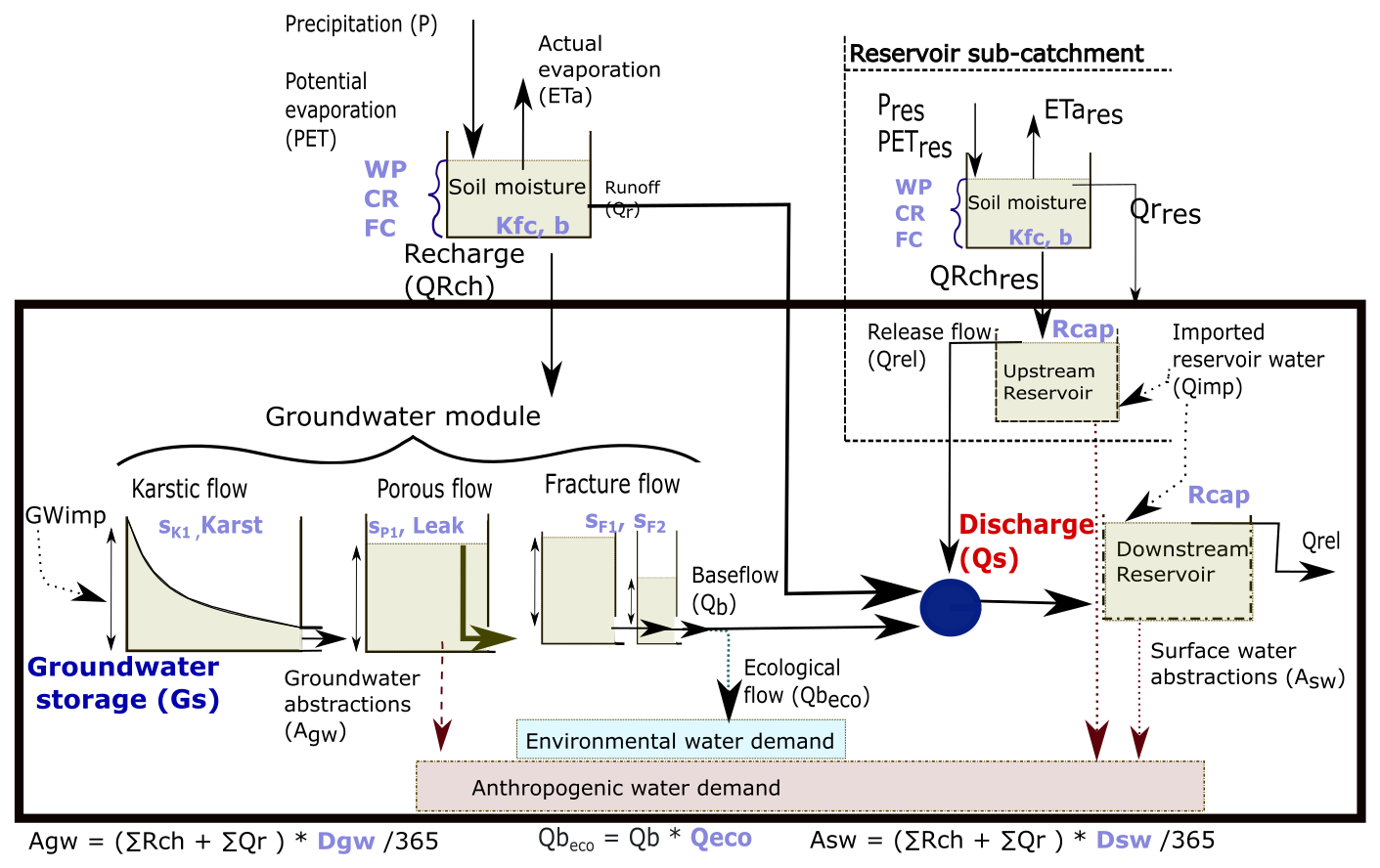
Figure 1 Model setup for socio-hydrological water resources (SHOWER) model, modified from (Wendt et al., 2021). Represented fluxes include precipitation (P), potential and actual evaporation (PET and ETa), runoff (Qr), groundwater recharge (QRch), baseflow generated by one of three groundwater modules. These determine groundwater storage (Gs) of which demand for groundwater (Dgw) and abstractions (Agw) are taken. Discharge (Qs) is the sum of runoff, baseflow (Qb) and release flow (Qrel) in case of an upstream reservoir setup (depending on the contributing area) or only runoff and baseflow in the case of a downstream reservoir. Surface water demand (Dsw) and abstractions (Asw) are taken from either the upstream or downstream reservoir.

As shown in Fig. 1, SHOWER is driven by daily climate data, i.e. precipitation (P) and potential evaporation (PET). Non-evaporated precipitation (ETa) fills the soil moisture balance and soil characteristics determine how much of this water is runoff (Qr), stored or passed on to the groundwater component as recharge (QRch). SHOWER has three groundwater modules representing karstic, porous and fracture flow which are modelled using modified lumped approaches (Stoelzle et al., 2015). Using one of the three groundwater-outflow modules, stored groundwater (Gs) can be released as baseflow (Qb). In the karstic module, baseflow release follows a power law. The porous module accounts for slow baseflow release with a small (7 %–12 %) leakage factor and baseflow in fractured aquifers is modelled using two parallel linear buckets (Stoelzle et al., 2015). Discharge (Qs) is taken as the sum of baseflow, runoff and release flow (Qrel) if there is an upstream reservoir. The upstream reservoir catchment is defined by calculating the reservoir contributing area and is modelled as a percentage in the (semi-)lumped catchment approach. The percentage divides the driving data into contributing (reservoir sub-catchment in Fig. 1) and non-contributing precipitation and potential evaporation (Salwey et al., 2023). Consequently, two soil moisture balances are calculated which lead to different discharge and groundwater outputs. Water demand is calculated as a proportion of the long-term recharge and runoff (all water that enters the black box in Fig. 1). Anthropogenic water demand can be divided between either surface water (Dsw) or groundwater (Dgw) and is abstracted from the surface water reservoir (Asw) and groundwater storage (Agw).

Water management impact is modelled using four separate drought management scenarios that are compared to a baseline scenario, which influence all fluxes in the black box in Fig. 1. In the baseline scenario there are no water management interventions and surface and groundwater water demand are simply abstracted from the reservoir and groundwater storage. The other four drought management scenarios were defined in Wendt et al. (2021) and represent common drought management practices in the UK. The first is to increase groundwater supply, using more of (underused or old) licenced groundwater boreholes and the natural storage buffer that aquifers provide. The second is to reduce water demand, which often starts early with a media campaign to stimulate lesser or limited water use by the public. Severe measures can, however, restrict water use for commercial or non-essential public water use. These threshold-based scenarios (following drought triggers) depend on the severity of a meteorological and/or hydrological drought. Measures are often introduced gradually and their severity increases depending on thresholds for precipitation, discharge, reservoir or groundwater storage levels that are related to historical drought events (for details see Wendt et al., 2021). The next two scenarios apply regardless of a defined drought and are integrating surface water and groundwater use. The third scenario manages surface water and groundwater in conjunction depending on which resource has a higher availability at a time. For example, in areas with large groundwater storage, more groundwater is used compared to surface water and vice versa for areas with low groundwater storage. In practice, this requires high flexibility in management operations. The last scenario aims to preserve ecological minimum flows in rivers by reducing surface water abstractions. Water is taken from groundwater instead.

We have modelled the threshold-based scenarios using average thresholds for precipitation, discharge, reservoir and/or groundwater levels, following Wendt et al. (2021). For the first scenario, we increased groundwater use whereas in the second scenario both surface water and groundwater are reduced equally. The third scenario integrates water storage and takes water from the highest store (either groundwater or reservoir storage) to meet water demand. This represents a non-restrictive application of conjunctive use practices. The last scenario maintains a threshold (Qb_eco) for the ecological minimum flow from baseflow (plus the release flow from an upstream reservoir, if present) and groundwater demand is ceased when this threshold is reached. In the case of water demand exceeding reservoir and groundwater storage, water can be complemented by imported water as either a fixed share or conditionally on (reservoir or groundwater) water levels (Qimp and GWimp).

2.2 Response-based model evaluation

The response-based model evaluation consists of a Global Sensitivity Analysis to determine the sensitivity of the model outputs to variations of the model parameters. The goal is to evaluate the consistency of the model behaviour with our understanding of key simulated processes, by checking that the “right” parameter controls the “right” output at the “right” time. For such analysis, parameters are sampled from ranges that are meant to represent the variability of hydrological characteristics across Great Britain – called “national parameter ranges” from now on.

2.2.1 Definition of the national parameter ranges

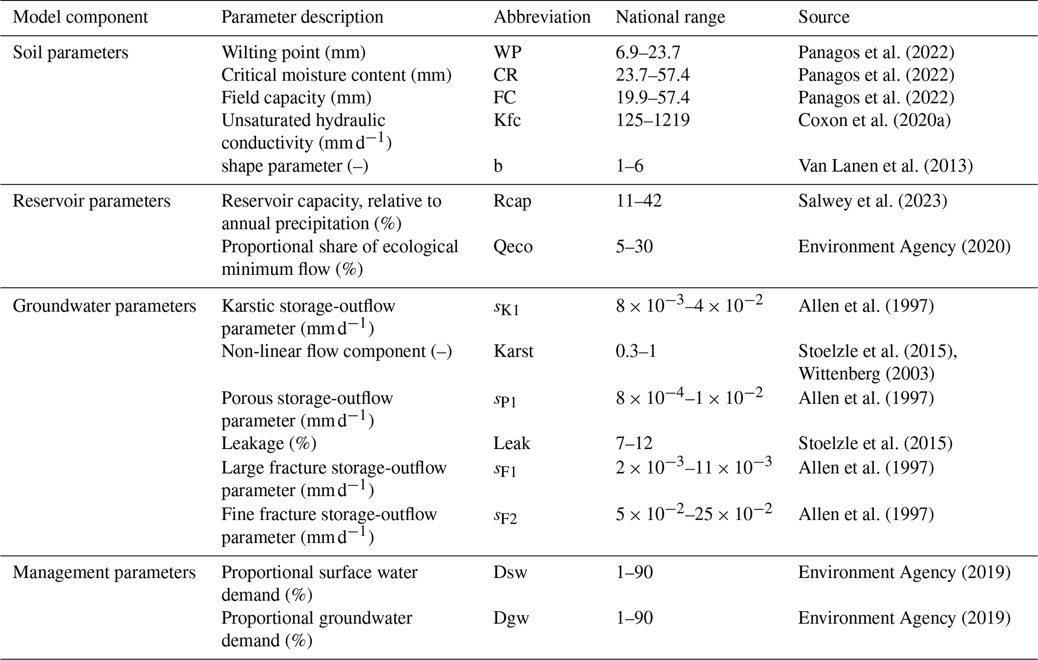
The four model components of SHOWER use 15 parameters, listed in Table 1. In total there are 11 model parameters active at one time, as only one of the three groundwater modules is activated for a simulation. For most of these model parameters (13 out of 15) we could identify a range of variability for Great Britain (fourth column in Table 1) based on scientific literature and open-source data. For the remaining two parameters, the critical moisture content (CR) and flow shape parameter (b), we could not find a national reference and thus will use the theoretical ranges. National ranges for soil characteristics (wilting point (WP) and field capacity (FC)) were based on the European soil dataset (Panagos et al., 2022). The range for unsaturated hydraulic conductivity (Kfc) was based on CAMELS-GB (Coxon et al., 2020a), from which we also used the long-term mean (1999–2014) abstraction values (Agw and Asw) that were converted into relative abstractions using the long-term recharge (P-PET for this time period). Reservoir capacity ranges were calculated using the range of Normalised Upstream Capacity values from Salwey et al. (2023), which describes the capacity of the reservoir (how much water can be stored) with respect to the catchment area and mean annual precipitation. Since the range presented in this paper is for the national distribution of reservoirs (and therefore contains several outliers) here we use the upper (Q75) and lower (Q25) quantile ranges of Salwey et al. (2023). The Environment Agency provides recommendations for ecological minimum flows (Qeco) thresholds, which were used to model both release flow from the upstream reservoir and the ecological flows from baseflow (Environment Agency, 2020). Finally, groundwater storage-outflow (s) parameter ranges were sourced from Allen et al. (1997) and expanded to include tested modelling parameters used by Stoelzle et al. (2015) and Wittenberg (2003).

Panagos et al. (2022)Panagos et al. (2022)Panagos et al. (2022)Coxon et al. (2020a)Van Lanen et al. (2013)Salwey et al. (2023)Environment Agency (2020)Allen et al. (1997)Stoelzle et al. (2015)Wittenberg (2003)Allen et al. (1997)Stoelzle et al. (2015)Allen et al. (1997)Allen et al. (1997)Environment Agency (2019)Environment Agency (2019)

Table 1 National parameter ranges for SHOWER parameters in each model component. All the ranges are taken from open-source datasets or sources (see last column) and ranges were specified to represent England using spatial datasets (Panagos et al., 2022; Coxon et al., 2020a), based on research in England (Salwey et al., 2023; Allen et al., 1997) recommendations for water managers (Environment Agency, 2019, 2020) or international studies specific to this modelling approach (Van Lanen et al., 2013; Stoelzle et al., 2015; Wittenberg, 2003).

2.2.2 The Global Sensitivity Analysis approach

The GSA considers several output metrics: the mean simulated discharge, the mean relative groundwater storage, and three key characteristics (duration, intensity and frequency) of simulated groundwater droughts. The GSA is used for a response-based evaluation of the model and is not specific to any catchment. Hence we used a central location in England to generate “average” climate conditions for GB (Wendt et al., 2021) derived from gridded climate data (HadUKP, Alexander and Jones, 2001, and CHESS-PE, Robinson et al., 2016; 1980–2017). Climate forcings for this central point were used in all Monte Carlo simulations against a sample of 10 000¹ parameter combinations. For each output metric, we used the PAWN method (Pianosi and Wagener, 2018b) to calculate the (global) sensitivity indices, each measuring the relative importance of a model parameter in controlling the variability of that output metric. All calculations were performed using the R version of the SAFE toolbox (Pianosi et al., 2015). Specifically, we performed three analyses: (1) a time-varying analysis to investigate changes in discharge and groundwater storage sensitivity over time; (2) an overall sensitivity analysis of time-averaged discharge and groundwater storage to management scenarios; and (3) an analysis for drought characteristics specifically.

In the first analysis, we quantify the sensitivity of simulated discharge and groundwater storages averaged over a 7 d moving window over the nearly 40 year period. This allows us to track the relative importance of the model parameter over time. The primary aim of this evaluation is to identify which model output is sensitive to which parameters and at what times, as this provides information about known (coded) and unknown (cross-)dependencies of model outputs. Parameters are considered non-influential if their PAWN score is less than the error of the sensitivity indices (Pianosi and Wagener, 2018a). The second analysis focuses on the overall influence of management scenarios on the mean discharge and groundwater storage (i.e. averaged over the entire simulation period). Lastly, the third analysis focuses on the influence of the modelled drought management scenarios on three key characteristics (duration, intensity and frequency) of simulated groundwater droughts. Drought events were identified as periods during which the simulated groundwater storage time-series fell below the 20th monthly varying threshold (Hisdal et al., 2024). Only droughts with a minimum duration of at least 30 d were considered. For each drought event, we quantified the difference in duration (in days), maximum intensity (in mm) and occurrence (count) between the simulation under a given drought management scenario and a baseline simulation with the same parameter set. Using these differences we could analyse how drought characteristics changed using the same (physical) parameter inputs and only changing the management strategy.

2.3 Study area and catchment selection

For the data-based model evaluation, we first selected representative regions in the UK that captured typical groundwater typologies, which were matched with the groundwater-outflow modules in SHOWER. One study region is set in the Chalk aquifer, which is represented using a large groundwater storage with dominant karstic, non-linear, flow characteristics (Hartmann et al., 2015; Wittenberg, 2003). The second study region covers the Permo-Triassic Sandstone aquifer using the medium groundwater storage with throughflow in the porous aquifer (Shepley et al., 2008). Lastly, quick and shallow groundwater storage is modelled using the smaller groundwater storage, reflecting the Dinantian Limestone aquifer with predominantly fracture flow releasing groundwater storage (Allen et al., 1997).

Approximately 40 % of all CAMELS catchments (671) are located on one of these productive aquifers, but groundwater level data from the Hydrology Data Explorer (Environment Agency, 2024) were only available for a third of those CAMELS catchments. From these 103 overlapping CAMELS catchments, we identified catchments that had one substantial type of abstraction (surface water or groundwater) and minimal wastewater discharges (<10 % of discharge) in order to evaluate the management components in SHOWER.

The selected three catchments are shown in Fig. 2. The first catchment (C1) is set in the Peak district in the Dinantian Limestone aquifer area (Derwent river catchment, 335 km²; CAMELS ID: 28043), which is reported to have 25 % of recharge abstracted via surface water (Coxon et al., 2020a). These abstractions are likely to come from the large upstream reservoir (Ladybower) that affects discharge time series downstream (Salwey et al., 2023). The second catchment (C2) in the Trent river catchment (163 km²; CAMELS ID: 28052) is located in the more urban midlands on top of the Permo-Triassic Sandstone aquifer. Groundwater abstractions are reported to be equivalent to 26 % of long-term recharge (P-PET) (Coxon et al., 2020a). The last catchment (C3) is the Pang river catchment (121 km²; CAMELS ID: 39027) located in Southern England in the Chalk aquifer where groundwater abstractions are approximately 30 % of long-term recharge.

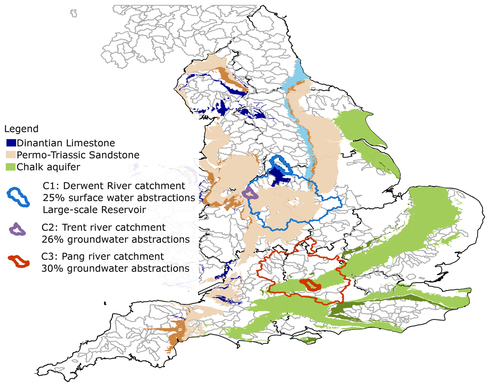
Figure 2 Map of the three selected CAMELS catchments that overlay three productive aquifers (the Dinanian Limestone, Permo-Triassic sandstone and Chalk) and have one substantial proportion of recharge taken via licenced surface water or groundwater abstractions. Both C1 and C2 are located in the larger Trent river catchment (in thin dark blue CAMELS ID: 28009) with Derwent catchment (C1 CAMELS ID: 28043 in blue) and upstream Trent catchment (C2 CAMELS ID: 28052) in purple. The larger Thames catchment (CAMELS ID: 39001) is indicated dark orange with the modelled Pang catchment (C3 CAMELS ID: 39027) in orange. Contains data from Coxon et al. (2020a). This dataset is available under the terms of the Open Government Licence.

2.4 Data-based model calibration and evaluation

The data-based model evaluation examines modelling performance in matching historical discharge and groundwater level observations in the three case study catchments over a 10 year period (1994–2014). We used CAMELS-GB daily climate time series to run SHOWER in each of the three case study catchments (Coxon et al., 2020a). For each catchment, we run the model against 10 000² randomly sampled parameter combinations over the first half of the available records (1994–2003), which we used as calibration period. Simulations were compared to observed discharge (in mm d⁻¹) from CAMELS-GB. Observed groundwater levels (moAD) were matched with CAMELS-GB catchments using the Hydrological Data Explorer (Environment Agency, 2024) and then normalised to vary between zero (lowest observation) and one (highest observation). When multiple observation wells were present in the same catchment, normalised groundwater values were averaged across wells. Even though averaging levels across wells simplifies the groundwater representation, an immediate benefit is that missing or deleted suspected (flagged) groundwater level observations were not a modelling constraint. Groundwater level time series with large sequences of suspected faulty (flagged in Environment Agency, 2024) observations were excluded from the study.

We used the modified Kling-Gupta Efficiency (Pool et al., 2018) to evaluate the model's performance for both discharge (KGE-Qs) and normalised groundwater values (KGE-Gs) in the calibration period. Additionally, we used the log Nash Sutcliff Efficiency (NSE_log) for modelled discharge to assess the model's ability to capture low flows. Based on calibration performance, we selected the top runs that maximised the model's fit to either discharge, groundwater or a “Best Overall”. The number of top performing simulations can be defined in multiple ways (e.g. top 100, or top 50 or top 20). We found a slight change in the improvement rate of NSE_log around the top 50, particularly in the Chalk simulation (see Fig. S2 in the Supplement) and therefore settled on using the top 50 simulations for the model evaluation. The Best Overall simulations were determined by the summed rank of the calculated NSE_log, KGE-Qs and KGE-Gs. The lowest numbers (highest rank) across the three performance criteria determined which simulations were considered “Best overall”. We used the top-performing parameter sets (25–50th percentiles) on the validation period (2004–2014) to check whether these parameter sets maintained good performance on a different dataset unseen during calibration. Last, we verified whether the top performing parameters so obtained fall into specific sub-ranges of the national parameter ranges of variability, and whether these sub-ranges are consistent with published catchment characteristics for each area. For soil parameters, we used catchment-specific information from CAMELS dataset Coxon et al. (2020a) and a range using the mapped European Soil database (Panagos et al., 2022). Reservoir information came from Salwey et al. (2023) and detailed groundwater storage information was found in Allen et al. (1997).

3 Results

3.1 Response-based model evaluation

The time-varying global sensitivity analysis shows consistent results for all parameters across the thirty years (reported in Figs. S4–S6 in the Supplement), of which we show a subset (2009–2014) with significant wet and dry periods in Fig. 3. In general, we find higher parameter influence in wetter periods compared to drier periods and higher sensitivity values for discharge compared to groundwater storage. Soil parameters, such as critical moisture content (CR) and field capacity (FC), control recharge and they are most notably influential during wet periods for both model outputs. The influence of these parameters on groundwater storage lasts for longer compared to discharge. Reservoir parameters are non-influential for the karstic and porous module, which is to be expected with a downstream reservoir setup. From the two groundwater parameters (sK1 and Karst), the parameter regulating non-linear flow (Karst) is very influential for discharge, particularly during high flows. The influence of the discharge-outflow parameter (s_K1) is relatively minor, particularly for groundwater, but this is a feature of the karstic module only as the discharge-outflow parameter in the porous (s_P1) is much more influential (see Fig. S7 in the Supplement). We also see more sensitive groundwater-outflow parameters in the Fractured module (s_F1 and s_F2) with the larger one (s_F2) being the most sensitive (see Fig. 4).

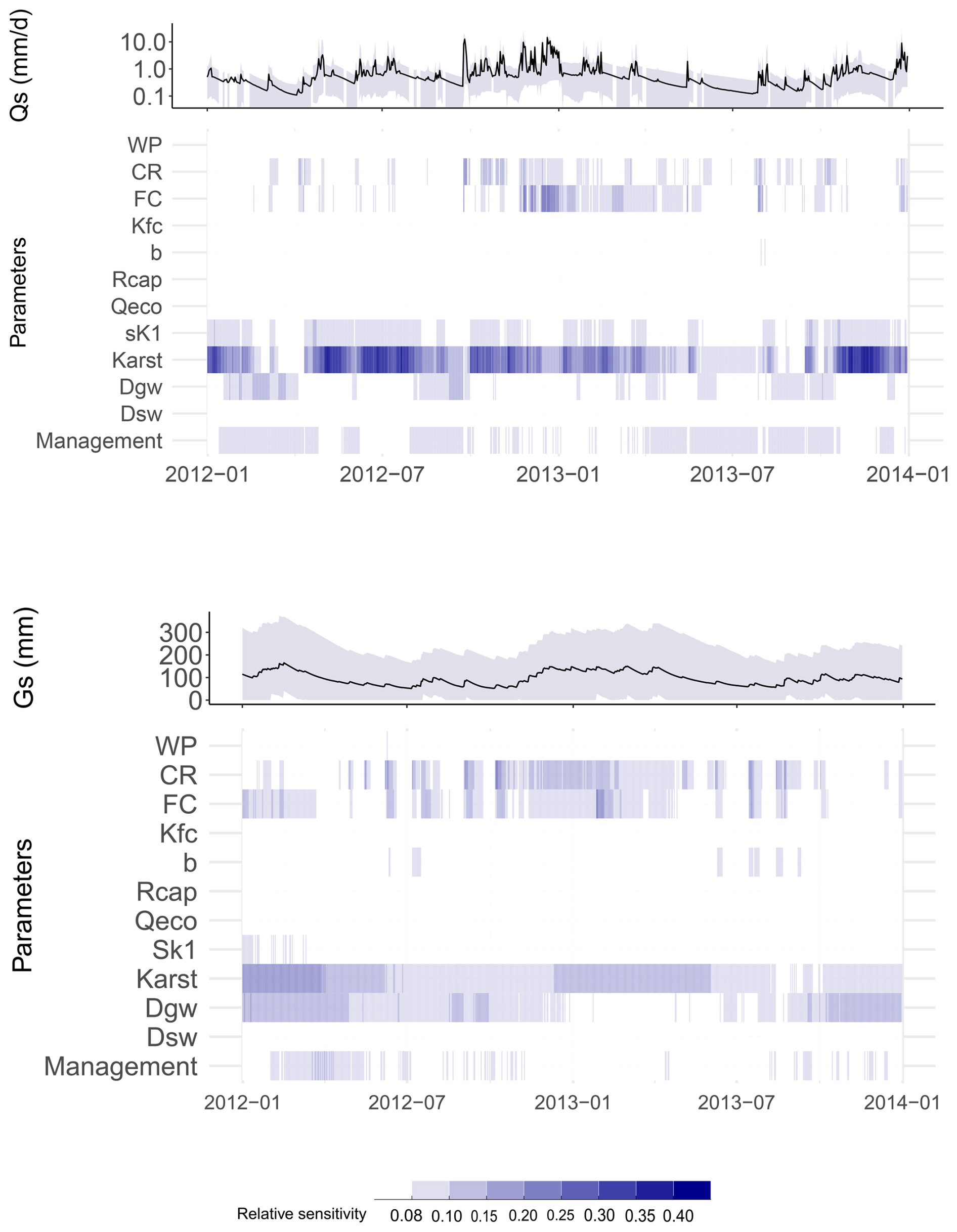
Figure 3 Time-varying sensitivity indices of the 12 parameters of the SHOWER model with a downstream reservoir setup (using karstic groundwater module) over the period 2012–2013. Output metrics are the mean discharge (top) and mean groundwater storage (bottom) averaged over a 7 d moving window. Discharge is plotted using a log scale. Mean discharge and groundwater storage are shown in blue, with their respective 10th and 90th percentile of the 10 K model simulations in light shading.

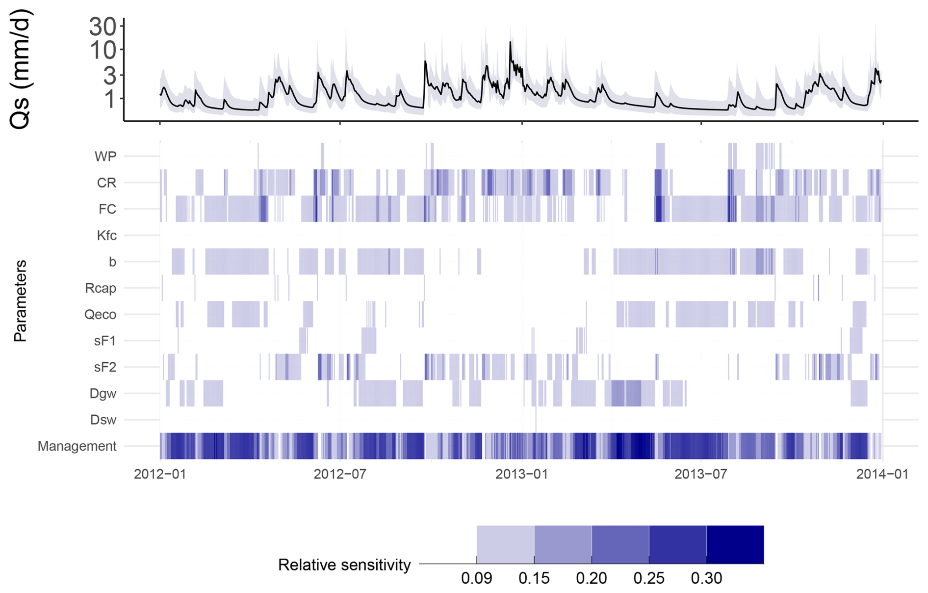
Figure 4 Time-varying sensitivity indices of the 12 parameters of the SHOWER model with an upstream reservoir setup (using fractured groundwater module) over the period 2012–2013. Output metrics are the mean discharge (top), which is plotted using a log scale. Mean discharge is shown in blue, with their respective 10th and 90th percentile of the 10 K model simulations in light shading.

Drought management scenarios are influential during flow recession and low groundwater storage, and non-influential during wet periods. When it is dry, both groundwater abstractions (Dgw) and scenarios (Management) become more influential compared to other dominant soil moisture parameters (CR and FC) and mostly determine the model output. The fractured module has, with its upstream reservoir setup, a different pattern with discharge being influenced by different parameters at different times (Fig. 4; groundwater in Fig. S8 in the Supplement). The shape parameter (b; in soil moisture module) and Qeco determining the ecological (and release) flow out of the reservoir are more influential during recession periods compared to the other groundwater modules. Interestingly, the reservoir capacity (Rcap) is only influential for specific days; when the peak flow is high and the maximum capacity is reached. The most sensitive parameters are associated with the drought management scenarios. Drought management scenarios are particularly sensitive during recessions and much less so when discharge peaks.

When analysing the overall sensitivity to the modelled drought management scenarios, we find that model outputs are significantly controlled by the chosen scenario, see Fig. 5. In this figure, we show the distributions of mean discharge (left) and mean groundwater storage (right) obtained by varying all model parameters within the national ranges, while maintaining a particular management scenario. The Figure shows different results for the two integrated water management scenarios (conjunctive use and maintaining ecological minimum flow). These two scenarios are managing water demand interchangeably between surface water or groundwater depending (1) on storage levels at a time (conjunctive use) or (2) baseflow relative to the ecological minimum flow (maintaining ecological minimum flow).

In the karstic and porous groundwater modules (A-B-C-D), the difference between the conjunctive scenario (in yellow) and the other scenarios follows a similar pattern. There are fewer zero flow conditions and higher flow occurrences when conjunctive use is applied compared to the baseline (in black) and other management scenarios (coloured). Overall groundwater storage is lower in the conjunctive use scenario compared to the other scenarios. This stark difference demonstrates the leverage of the conjunctive use scenario. Other scenarios show very little leverage as their influence relative to parameter uncertainty is small, with exception of the Ecological flow scenario that has a longer tail, indicating high flows more frequently occurring compared to the baseline.

In the fractured module (E-F), discharge and groundwater simulations show three distinct clusters. Drought management scenarios that are trigger-driven, such as increasing water supply or reducing water demand (in blue and red), move the discharge distribution towards the left along the x axis resulting in fewer low flow conditions and overall higher flows compared to the baseline (5E). This means that mean discharge is generally higher. Groundwater storage is lower for these scenarios. Integrated water management scenarios (conjunctive use and ecological minimum flow in yellow and green), also result in fewer zero flow occurrences but the distribution of high flows is more similar to the baseline. Integrated scenarios also result in fewer low groundwater storage conditions (Fig. 5F) and a clear increase in larger values, whereas drought-trigger scenarios are very similar compared to the baseline scenario.

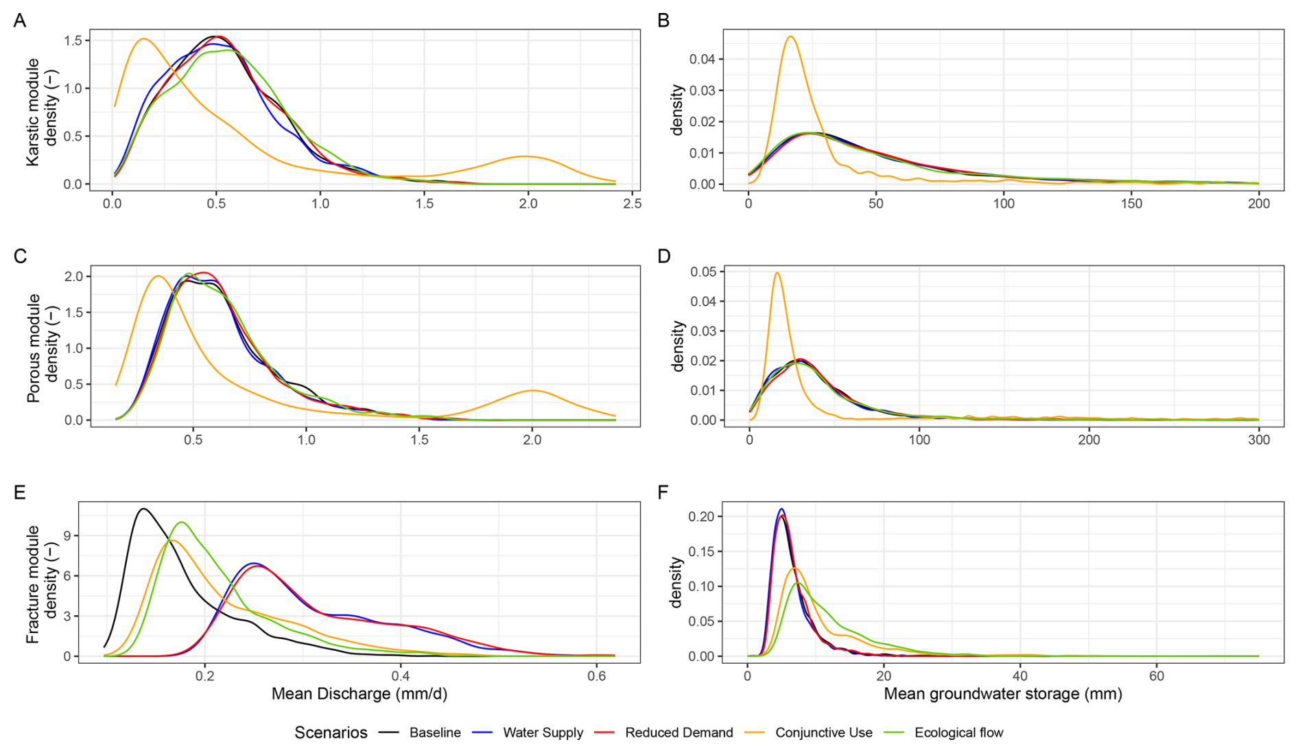
Figure 5 Distribution of simulated mean discharge (A, C, E )and mean groundwater storage (B, D, F) for the SHOWER model using the karstic module (A, B), the porous module (C, D) and the fracture module (with upstream reservoir) (E, F). Each distribution is obtained by varying all model parameters within the national ranges, while holding the drought management scenarios fixed to the baseline scenario (black lines), one of the two drought trigger-driven scenarios (blue and red) or one of the two integrated management scenarios (yellow and green).

The leverage of the modelled drought management scenarios is also reflected in the groundwater drought characteristics with drought deficit, i.e. the intensity of drought events being most sensitive (Fig. 6). This intensification of groundwater drought events is largely due to an overall lower groundwater level in the karstic and porous module (Fig. 5) following from the conjunctive use scenario. Detailed results highlight the strong negative difference between the baseline and the integrated management scenario (Figs. S9 and S10 in the Supplement). The overall influence on drought duration is positive, meaning shorter droughts, for most scenarios in the porous and fractured module. In the karstic module (and to some extent in the porous module) a larger spread of drought durations is found, which also reflects the increased sensitivity to groundwater demand under drought conditions for this specific aquifer type (Fig. 6). Again, the largest differences are found for the conjunctive use scenarios compared to the trigger-driven scenarios (Figs. S9–S11 in the Supplement).

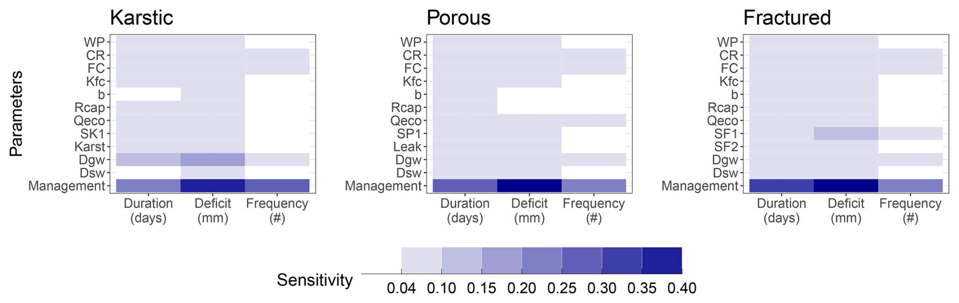
Figure 6 Sensitivity indices of the SHOWER model parameters (in the 3 configurations using Karstic, Porous and Fractured groundwater modules) for three output metrics: mean duration, mean deficit and frequency of groundwater drought events.

The distinct difference in leverage in fractured module between the trigger-driven and integrated drought management scenarios is mostly reflected in the drought frequency, as drought intensity and duration follow the same pattern – but less strongly negative/positive compared to the other groundwater modules. The smaller differences compared to baseline might be due to the overall higher groundwater storage levels in the integrated scenarios (Fig. 5). The increased water supply and reduced water demand scenarios in/decrease drought frequency respectively. Integrated scenarios result in a large range in drought frequency with maintaining hands off flow scenarios slightly reducing overall frequency (Fig. S11).

3.2 Data-based model calibration and evaluation

Figure 7 shows the distribution of model performance over the calibration period according to different metrics. In all three catchments, we find consistent results between calibrating to fit discharge observations (KGE-Qs or NSE_log), groundwater observations (KGE-Gs) or a “Best Overall” (combined ranked performance criterion). The range in performance between the calibration approaches varies for the catchments and we find a trade-off between calibrations on either discharge, groundwater or both model outputs.

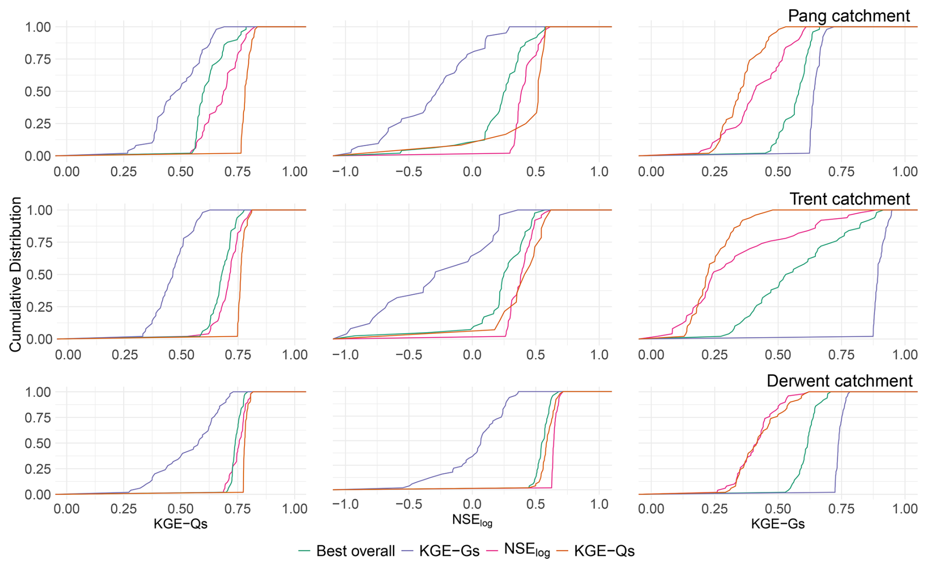
Figure 7 Distribution of model performance shown for the three catchments (Pang, Trent and Derwent). In each plot the four calibration approaches are shown (coloured). The three columns show the top 50 results measuring the KGE for discharge (KGE-Qs), the logged NSE of discharge (NSE_log) and the KGE for groundwater (KGE-Gs).

The first calibration strategy is using only discharge (based on KGE-Qs) and results in slim ranges for all catchments: Pang (0.75–0.81), Trent 0.76–0.84) and Derwent (0.77–0.82). These ranges are larger when fitting to NSE_log, Best Overall or groundwater-only calibration strategies, see first column in Fig. 7). These discharge-only calibrations translate in considerably less reliable results for groundwater storage (KGE-Gs: 0.13–0.62). Low groundwater storage conditions are typically under-represented resulting in a lower KGE-Gs. In the NSE_log scores (middle panel in Fig. 7) we see the same pattern with the best scores for calibration on discharge droughts (based on NSE_log) and KGE-Qs. Capturing the drought periods in discharge seems more appropriate when applying the NSE_log criteria that result in scores ranging between 0.61 and 0.71 for all catchments.

In groundwater-only calibrations, KGE-Gs for groundwater can be very high and narrowly confined with scores ranging between (0.62–0.95; see last column in Fig. 7). As found before, discharge-only calibration approaches result in a larger range for KGE-Qs (0.27–0.73) for all catchments. NSE_log scores for discharge are largely negative, suggesting this method is less suitable to represent discharge droughts. The “Best Overall” approach that combines all the performance criterion results in larger performance ranges for both model outputs, although score ranges are largely acceptable for both discharge (0.55–0.79; first column) and groundwater (0.27–0.91; last column).

In Fig. 8, we show the time series of simulated discharge and normalised groundwater storage over the validation period 2004–2014 for the Pang catchment, for the four calibration approaches. Coloured lines are simulations from the top 50 calibration results based on NSE_log (pink), on KGE-Qs (purple), and on the Best Overall metric (green). The model calibrated to discharge observations (pink) has an overall good performance despite some exaggerated high flows within this period. The overall seasonality and recovery to normal flow conditions is particularly well-captured in 2007 and 2011 in this heavily-abstracted Chalk catchment. The model calibrated with “Best Overall” criterion produces less good simulations with frequent underestimations of low flows. This is however a feature of the Chalk only, as validation time series of the Trent show well-captured low flows (Fig. S12 in the Supplement). Observed low flows in the Derwent are consistently lower compared to simulations, which might be due to simulations flattening out on an ecological flow between 5 %–30 % of baseflow (Fig. S13 in the Supplement). Groundwater time series are remarkably similar between the KGE-Gs and “Best Overall” calibration in the Chalk (Fig. 8, others in Figs. S12 and S13). Both calibrations result in well-captured periods of declining and low groundwater storage in 2004–2006 and 2010–2012 with a slight overestimation in 2007–2008 compared to the mean observed groundwater storage (dotted).

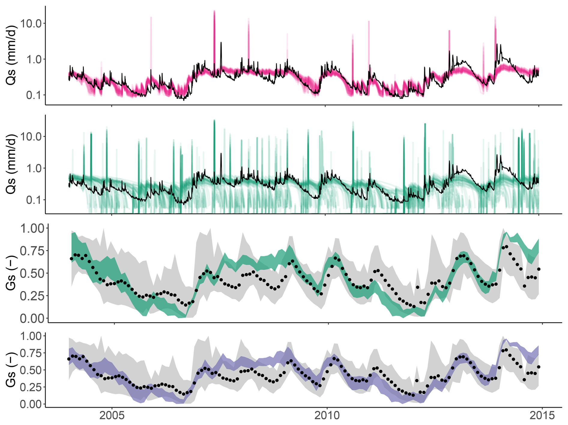
Figure 8 Simulated discharge (Qs (mm d⁻¹)) and normalised groundwater storage (Gs (–)) in the Pang catchment over the validation period 2004–2014. Top panel shows discharge simulations calibrated on NSE_log (in pink) and the middle panels shows discharge calibrated on the “Best Overall” criteria (in green). The lower panels show normalised groundwater simulations calibrated on the “Best Overall” (in green) and KGE-Gs (in purple). Black lines/dots are observations. Note that groundwater level observations are averaged from 17 locations, with the range of variability across the stations in grey.

Finally, we investigate the values of the top 50 performing parameter sets for the “Best Overall” calibration across the three catchments. In Fig. 9 each of these 50 parameter combinations is represented by a grey line. On top of these lines, box plots help visualise the spread of these “optimal” parameter values. Overall, we see that calibration highly constrains the three soil moisture parameters (WP, CR and FC) in all three catchments. In the Pang catchment, the non-linear flow (karst) and groundwater abstraction parameter (Dgw) are also well constrained; and so are discharge-outflow parameters s_P1, s_F1 and Dgw in the Trent and Derwent catchment. Interestingly, in the Derwent catchment even more parameters (i.e. Kfc, b, Rcap and Dsw) are constrained compared to the Pang and Trent, which is likely due to the upstream reservoir setup which heavily influences discharge in the Derwent.

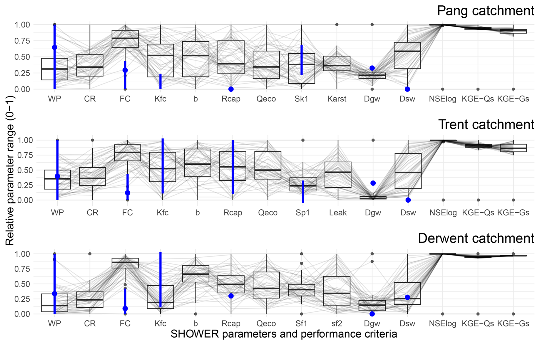
Figure 9 Parallel coordinate plots for the Pang, Trent and Derwent catchments, which show the top-50 parameter sets according to the “Best Overall” performance criteria (grey lines). The range of the parameters is presented relative to the national range (see Table 1) used for sampling. The last columns show the performance criteria NSE_log, KGE-Qs and KGE-Gs associated to each parameter set. Box plots help visualise the spread of the grey lines. Blue lines/dots are the expected parameter ranges/values purely based on catchment-specific information.

Parameters that are hardly constrained by the calibration vary for the three catchments. With an upstream reservoir setup in the Derwent, there are just two almost unconstrained parameters (Qeco and s_F2), i.e. where top 50 values are almost evenly spread over the national range used for sampling. In the Pang and Trent, soil parameters such as the unsaturated hydraulic conductivity and shape parameter (Kfc, b) are also unconstrained, as are the reservoir capacity, ecological minimum flow and surface water demand parameters (Rcap, Qeco, and Dsw respectively), which are all affecting the downstream reservoir.

The blue bars (or dots) in Fig. 9 indicate the expected ranges (or point-values) of the model parameters based on local information about the catchment characteristics (where available). In some cases (wilting point WP and unsaturated hydraulic conductivity Kfc in the Trent and Derwent catchment), these ranges are as large as the national ranges, derived from the CAMELS catchment attribute data (Coxon et al., 2020a) and the European Soil database (Panagos et al., 2022). For other parameters, such as groundwater storage data, calibrated values are similar to what we expect/know about the catchment. Data detailed for the Kennet Valley and Stafford basin (Allen et al., 1997) is largely in agreement with the calibrated values. In the Pang, proportionate groundwater demand (Dgw) is calibrated consistently to expected value of 30 % (based on (Coxon et al., 2020a)). However, in the other catchments, calibration yields parameter values lower (Trent) and higher (Derwent) than expected based on local information. For the field capacity parameter (FC) we identified a disagreement between calibration and local information (from both CAMELS and the EU database) in all catchments. The calibrated Reservoir capacity (Rcap) in the Derwent catchment is also slightly larger than the capacity of the Ladybower reservoir (from Salwey et al., 2023). For the Trent, calibrated ranges for Rcap are as large as the blue range, as this information is only available for the larger Trent catchment (CAMELS ID 28009; also shown in Fig. 2).

4 Discussion

4.1 SHOWER Model Performance

Overall, SHOWER simulations perform well in terms of baseflow and groundwater storage simulations in the three diverse groundwater-rich catchments analysed here. Despite the difficulty of capturing droughts and low flows using a bucket model (Melsen and Guse, 2019), we have shown that calibration focused on low flows (using NSE_log as performance criteria) lead to capturing low flows well also in the validation period.

The SHOWER performances reported in this paper are comparable or exceed the results of other hydrological models for the same catchments. The largest improvements (measured in KGE) are found for the surface water-dominated G2G model (Hannaford et al., 2023b) where SHOWER improves the negative (Pang) and average (Derwent) KGE values. Other rainfall–runoff models, such as GR4J and GR6J yield similar results for their selected best runs in the Pang and Derwent catchments (Hannaford et al., 2023a), although the authors indicate that groundwater-dominated catchments are problematic to model well. The recent coupled DECIPHeR-GW model results are similar to those of SHOWER (Zheng et al., 2025), showing that adding the elaborate groundwater representation in this new DECIPHeR version improves model results for these areas (Coxon et al., 2019; Lane et al., 2021). Even for similar modelling performances, a key advantage of SHOWER is that it explicitly accounts for groundwater and surface water abstractions and reservoir influence, which introduces the possibility of testing the impact of management strategies, which is not possible using the previously mentioned models.

Similar to Zheng et al. (2025), SHOWER has the ability to simulate both discharge and groundwater output. Groundwater results are indicative of catchment's mean storage, as modelled groundwater storage is relative and spatially uniform (lumped). Despite this simplification, we show that groundwater time series can be well-captured using SHOWER (KGE: 0.62–0.95) for both combined and groundwater-only calibration criteria. We could however not compare these performances to those of other models, as published UK groundwater results are either not open-access and/or at the right scale (Mackay et al., 2014; Lewis et al., 2018; Bianchi et al., 2024; Rahman et al., 2023; Zheng et al., 2025). The dual model output does complicate a standard calibration process, as model users might want to identify priorities for their model use and could adjust the calibration accordingly to optimise performance or with the aim to find a single set of parameters. Presented calibration strategies do however not have substantial trade-off, as we have shown in the response-based evaluation that both surface water and groundwater can be well-captured in both wet and dry conditions (Kollat et al., 2012). The range in performance shown in Fig. 7 illustrates how various calibration strategies differ within capturing the overall flow variability and low flow conditions. Peak flows are however less well-captured when looking at high flows in 2010 in Fig. 8, which is to be expected with groundwater modules focusing on base flow generation (Stoelzle et al., 2015). It might also be a consequence of using KGE and logged NSE as calibration criteria, which do not specifically emphasise high flow conditions (Althoff and Rodrigues, 2021). Overall, benefits of the dual model output translate into a “Best overall” parameter set that can be used to produce both discharge and relative groundwater storage with reasonable confidence. This could overcome data availability issues in ungauged discharge catchments or unavailable (recent) groundwater level records.

4.2 Influence of management scenarios

Our results show that integrated drought management scenarios have the most leverage on the SHOWER model outputs, and particularly the conjunctive use scenario. Discharge and groundwater results are significantly altered by management scenarios, particularly during drought periods. The impact of modelling a particular management scenario dominates discharge and groundwater level simulations, as this impact exceeds model parameter uncertainty. Even though these are theoretical drought management simulations, results indicate a substantial influence regardless of the parameters used within the national range. In practise, there will be a combination of drought management strategies applied in a catchment at the same time and drought strategies will be adapted to reflect specific operations. For example, we applied a theoretical application of conjunctive use in which water use is fully integrated and non-restrictive. This approach is in line with large conjunctive use schemes where a range of water sources is used and the increased flexibility within a water distribution system increase drought resilience (Shepley et al., 2009; Scanlon et al., 2016; Seo et al., 2018). The modelled surface water imports represent the common cross-company water transfers that are an additional tool to overcome (short-term) water shortages. These are commonly used when approaching low reservoir storage (Wendt et al., 2021) but likely used prior to reaching the 25th threshold as water is frequently transferred between regions to increase resilience high water demand or droughts (Dobson et al., 2020). These local and regional water transfers can also be used to maintain ecological minimum flows (Environment Agency, 2019). How a combination of these modelled measures translate to better protection of ecosystems can be complex to observe on the ground. It will also require more site-specific modelling efforts, particularly investigating the water quantity aspect of water resources management interventions, as maintaining specific surface or groundwater levels via conjunctive or augmentation schemes does not directly guarantee a “good” ecological status (Jakeman et al., 2016; Murgatroyd et al., 2022).

The notable influence of these integrated water management strategies on drought characteristics (Fig. 6) is encouraging, but further research regarding the effectiveness of strategies is needed. Results indicate shorter drought durations by applying integrated management strategies with a mix of both intensified and relieved drought intensity particularly in the karstic and porous groundwater module. Additionally, the impact of demand measures that are widely applied in England, are most effective in a fast-responding shallow (fractured) groundwater module but less so in other groundwater modules, which emphasises the wider need for research. These measures are rarely modelled at scale (Murgatroyd et al., 2022) or investigated in a larger policy context (Urquijo et al., 2017). Alternative strategies to identify management impact use paired events, and show the positive impacts of drought and flood measures implemented at location of two UK case studies (Kreibich et al., 2022). How current and future drought management strategies hold against future UK heatwaves, increased water demand and increased effort to maintain low flows is receiving increasingly more attention. Not only because extensive modelling work is required to assess drought resilience at scale (Murgatroyd et al., 2022), but also because results indicate that without “further interventions to reduce water demand and provide additional water supplies, there is a high risk of water shortages, in particular in the South East of England.”

4.3 Intended use of SHOWER

SHOWER is designed for simulations of discharge, primarily baseflow, and indicative groundwater storage variations over time. SHOWER can be used as a screening tool to evaluate the impact of groundwater abstraction strategies on hydrological droughts. The model runs quickly in R (1–4 s per run on a Core i7 Intel laptop) and this provides the benefits of allowing on-the-fly calculations and what-if scenario analysis considering multiple combinations of parameters and/or management settings. SHOWER sits herein, in terms of mathematical complexity, between other bucket model approaches and (semi-)distributed models producing discharge (Bell et al., 2007; Coron et al., 2017; Coxon et al., 2019). A crucial difference is that SHOWER aims to represent groundwater-rich areas and is particularly well-placed to analyse droughts and drought management strategies in regions with significant groundwater contributions to streamflow. Groundwater storage is represented in relative terms and lumped for each catchment, meaning that results are simplified compared to distributed groundwater models, such as Lewis et al. (2018); Mackay et al. (2014); Rahman et al. (2023), and Bianchi et al. (2024). However, this simplification creates the opportunity to explore results droughts and management impact in more detail prior to investing in expensive detailed groundwater models. Moreover, the leverage of integrated drought management strategies shows the potential for SHOWER in decision-making processes and the modular, open-source model structure allows for adjusting SHOWER to local/relevant characteristics for a particular water management scenario/setting.

Possible model improvements to the current version might be relevant to users that focus on particular areas with impermeable surfaces or complicated land use areas (large urban areas), as SHOWER does not account for any differentiation in the soil characteristics or for urban water strategies (such as large sewage treatment works, Coxon et al., 2024). Other hydrological models also deploy more sophisticated soil modules and we would recommend to either be aware of the simple setup or use the modular model structure of SHOWER to synchronize in/outputs with alternative models. For small to medium-sized catchments, we have found that SHOWER is quick to setup and can simulate both discharge and groundwater storage. However, the absence of a routing module affects its performance for large catchments (approximately ≥1000 km²). Again, we would advise model users to either insert a routing module into the modular open-source structure of SHOWER to account for this, or use the modular model structure to adapt SHOWER in alternative ways. With the specific modelling aim to represent baseflow and storage in groundwater-rich areas, we acknowledge that SHOWER is a social construct to further hydrological drought management strategies in groundwater-rich environments (Melsen, 2022). However, the (open-source) modular structure of SHOWER, quick running time, and link with CAMELS-GB make for a versatile socio-hydrological model that could be applied to regions across the globe, using other CAMELS datasets (Addor et al., 2017; Fowler et al., 2021; Chagas et al., 2020) to support groundwater management decisions on the ground.

5 Conclusions

In this article, we present a socio-hydrological water resources modelling tool (SHOWER), which is designed to test hydrological drought management strategies. The focus of SHOWER is on groundwater-rich regions and to that purpose the lumped modelling approach includes three different groundwater-outflow modules. These are tested thoroughly in this work using a global sensitivity analysis (GSA). We also identified (un)influential parameters in the GSA that aided calibration when applying SHOWER to three case study areas in the UK. In this data-based model evaluation, we have shown how SHOWER can be deployed using open-source datasets to simulate both discharge and groundwater storage. Performance indicators show that both model outputs can reasonably fit historical observations, as we have demonstrated calibration results for (1) low flows, (2) only groundwater and (3) “Best Overall”. We have found good performance across three primary aquifers, showing how the three groundwater-outflow modules can generate baseflow whilst including water management interventions. We identified where local information could further constrain parameters and how further (local) data could be used to optimize model performance.

The GSA also indicated how modelled drought management strategies show leverage, meaning they have significant impact on model outputs beyond uncertainty of model parameters. Integrated water resource management scenarios such as conjunctive use and maintaining the ecological minimum flow showed significant improvement during droughts and with consistently higher flows and storage even when considering the full (national) parameter range. The consistent influence to both overall flows and hydrological droughts stimulates further research in these strategies. This could lead to further research in specific regions where water managers are looking to increase their integrated water management strategies and/or at regional level aiming to increase drought resilience strategies. With the modular and open-access structure of SHOWER we aim to provide a useful new tool for groundwater managers that they can use, modify and develop further to improve their work streams.