Return period analysis of weakly non-stationary processes with trends

Traditional return period analysis represents an essential tool for practitioners to assess the magnitude and occurrence of extreme events. The analysis considers stationary time series and assumes independent and identically distributed events. However, many environmental processes exhibit time-varying changes due to signal trends or shifts, leading to non-stationary behaviors. Although several approaches have been proposed in the literature and a formulation exists for the return period under non-stationarity, its practical use is often hampered by the long computational time. This work proposes a novel framework to estimate the return period by extending the simpler stationary formulation to weakly non-stationary processes, whose definition is derived by imposing a condition that limits the maximum change of the return period over a given timeframe. We rely on the General Extreme Value (GEV) distribution, allowing for time-varying parameters due to signal trends. The approach yields closed-form solutions for the maximum permitted trends in the GEV parameters (mean, variance, frequency, or magnitude) satisfying the weak non-stationarity hypothesis. Specific attention is paid to the case of the Gumbel distribution, for which the limit solutions are derived for the case of linear trends. We show that the approximation error is minor (approximately 5 % for the best tested parameters), compared to the more complex fully non-stationary solution, thus making the proposed framework a computationally efficient tool for practitioners.

1 Introduction

“Stationarity is dead” (Milly et al., 2008) or “stationary is immortal” (Montanari and Koutsoyiannis, 2014)? The statements reflect the fact that many environmental and hydrological processes exhibit time-varying changes of characteristic quantities, usually due to the presence of trends and shifts (Salas and Obeysekera, 2014; Obeysekera and Salas, 2016; Cancelliere, 2017), but such changes are usually observed in the short-term period, whereas the overall process may exhibit long-term stationarity (Fig. 1). In this regard, the term stationarity (also known as strict or strong stationarity) refers to the over-time steadiness of the probability distribution function (pdf) of the process (Katz, 2013). Mathematically speaking, we can write $p_X(X,t)=p_X(X,t+c)$, with p_X(X,t) the pdf of the process at time t, and c a constant. Accordingly, the steadiness condition can be written as $\partial p_X(X,t)/\partial t=\mathrm{0}$. Therefore, for strictly stationary processes, all the moments (e.g., mean, variance, skewness, etc.) of the p_X(X,t) function, as well as other statistical properties such as the above-threshold probability, are constant in time. When the time steadiness of p_X(X,t) moments is satisfied up to a particular order K, the process is Kth-order stationary and generally referred to as weakly stationary (Katz, 2013). For instance, if only the mean and variance are constant, the process is 2nd-order stationary. On the contrary, when the pdf varies in time such that none of the moments show over-time stationary, the process is defined non-stationary (see Fig. 1).

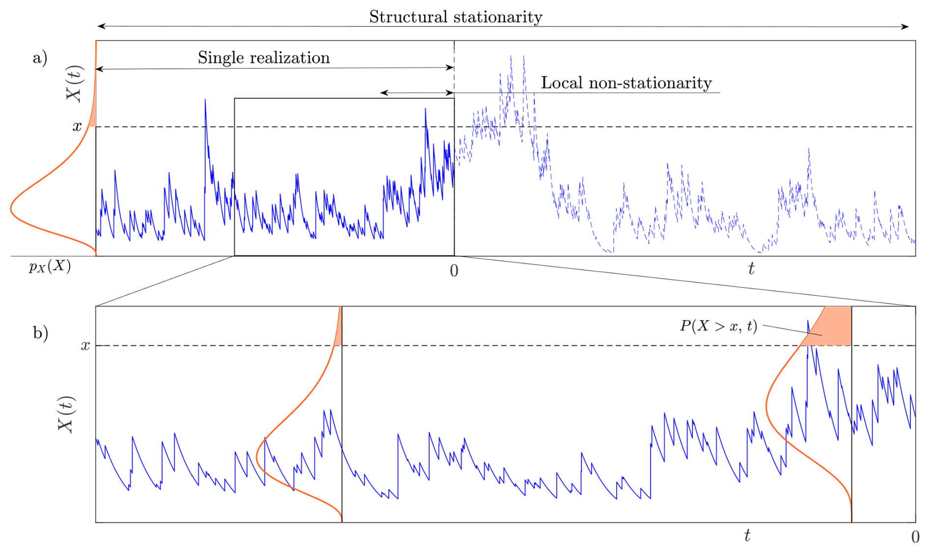
Figure 1 A sample realization of a structurally stationary Poisson-based stochastic process with constant parameters (mean frequency between events and mean jump magnitude) showing a local non-stationarity of long duration (continuous blue line) appearing up to the observation time (t = 0 y, present day). Dashed blue line represents a potential (unknown) future evolution of the process. Orange curves and shaded areas are the stationary, p_X(X), and non-stationary, p_X(X,t), pdfs and the cumulative probability, $P(X>x,t)$, above the threshold x (dashed black line), respectively. (a) A Compound Poisson Process with linear drift as a proxy for flow discharges in a river. Structural (long-term) stationarity is foreseen, but local non-stationarity arises in the short term. b) The cumulative probability above the threshold x changes when calculated according to short-term properties of the system's dynamics.

Regarding the specific case of hydrological and weather-related variables, several scientific studies have identified alterations of mean annual temperature, rainfall amount, and riverflow regime. The alterations in hydrological statistics are typically attributed to several factors, including natural variability of climate conditions, and systematic changes of the system's dynamics due to, for instance, anthropogenic activities (e.g., urbanization, land-use change, greenhouse gas emissions) which may impact the precipitation patterns, air temperature, and sea levels (Montanari and Koutsoyiannis, 2014; Koutsoyiannis and Montanari, 2015; Lee et al., 2023). Whether of climatic origin or not, significant changes also alter both the empirical and the theoretical probability distribution functions. For instance, Birsan et al. (2005) reported the presence of trends in the maximum flow discharge of Swiss rivers, which can be significantly correlated to the alterations in heavy precipitation events (Widmann and Schär, 1997) and temperature (Scherrer et al., 2016). Similar results were obtained in the analysis of mean precipitation data (Brunetti et al., 2000; Norrant and Douguédroit, 2006; Philandras et al., 2011), and sea level rise, both at the local scale (e.g., Galiatsatou et al., 2019, for an analysis of the Mediterranean area), and at the global scale (Church and White, 2011), as well as for the rainfall amount (New et al., 2001), and the streamflow regime (Lins and Slack, 1999; Douglas et al., 2000) in the United States.

From an engineering point of view, water resources management and the design of hydraulic structures rely on quantifying hydrological extreme events, like floods and minimal flows, and their duration. The traditional/historical procedure to estimate the extreme-event magnitude and the average occurrence frequency is based on the return period concept, which is defined as the average intertime between extreme events greater (lower) than, or equal to, a specific magnitude (threshold). Such a definition, usually implied in the design of engineering applications, is inherently built on the assumption of independent and identically distributed (iid) events above a specific value, x (i.e., the threshold). Therefore, the return period, $\stackrel{\mathrm{‾}}{T}\left(x\right)$, is usually taken as constant (in a stationary framework, as highlighted by the $\stackrel{\mathrm{‾}}{\cdot }$ notation) and associated with the time interval, Δτ, for which the observations are available (e.g., Δτ = 1 year, for annual observations). In terms of the occurrence probability of extreme events (with magnitude X≥x), the return period $\stackrel{\mathrm{‾}}{T}\left(x\right)$ can be calculated as:

$$\begin{array}{}\text{(1)}& \stackrel{\mathrm{‾}}{T}\left(x\right)={\displaystyle \frac{\mathrm{1}}{P(X\ge x)}}\mathrm{\Delta }\mathit{\tau }\end{array}$$

with P(X≥x) the exceedance probability related to extreme events (Fig. 1).

The iid hypothesis implies the over-time (strict) process stationarity, which is not satisfied in the presence of trends in the signal (Katz, 2013; Salas and Obeysekera, 2014). For instance, the return interval of a specific flood peak under non-stationary conditions can vary significantly over time, potentially ranging from thousands of years to less than a decade (Villarini et al., 2009). Noteworthy, when local non-stationarities or alterations in the observed statistical properties of the process dynamics are present (e.g., Fig. 1), the duration of the temporary changes must be much longer than the interval of observations (i.e., Δτ in Eq. 1), and specifically in the order of magnitude (e.g., decades) of the typical time-scales for engineering applications or other practical considerations involving design risk.

The analysis of extreme events has usually been performed by considering the annual maxima and the empirical definition of the occurrence probability of events above thresholds characterizing their extreme magnitude (Katz, 2013; Salas and Obeysekera, 2014). Some works additionally proposed the change of the return period definition, based on the expected waiting time until an event or the expected number of events over a given period, to better quantify the risk under non-stationarity (Volpi et al., 2015; Todini and Reggiani, 2024). As a consequence, the traditional quantification of extreme events based on the return period concept, such as the Peak Over Threshold (POT) analysis, is increasingly questioned (Cooley, 2013; Serinaldi, 2015; Read and Vogel, 2015; Vogel and Castellarin, 2017) and a proper framework that can dynamically account for the time-evolution of probability distributions is currently missing (Katz, 2013; Cooley, 2013; Salas and Obeysekera, 2014). Noteworthy, the change in return period due to shifts and trends may affect not only the peak values, but also time-integrated quantities. From a hydrological point of view, this condition may reflect in changes of the flow volume associated with a specific hydrograph and the duration of specific trajectories (mean first passage times) above, below, or between characteristic thresholds (Laio et al., 2001; Calvani and Perona, 2023, 2025). In the literature, some methods that involve a time-varying probability distribution (Fig. 1) have been formulated to address this challenge (Fernández and Salas, 1999; Obeysekera and Salas, 2016). According to Salas and Obeysekera (2014), the return period, ${\stackrel{\mathrm{̃}}{T}}_{\mathrm{0}}\left(x\right)$ at the current time (noted by the subscript 0) under non-stationary conditions (highlighted by the $\stackrel{\mathrm{̃}}{\cdot }$ notation) can be computed as:

$$\begin{array}{}\text{(2)}& {\stackrel{\mathrm{̃}}{T}}_{\mathrm{0}}\left(x\right)=\mathrm{\Delta }\mathit{\tau }\sum _{i=\mathrm{0}}^{\mathrm{\infty }}\prod _{j=\mathrm{0}}^{i-\mathrm{1}}\mathrm{1}-P(X>x,j\mathrm{\Delta }\mathit{\tau }).\end{array}$$

Due to non-stationary conditions, Eq. (2) defines the return period ${\stackrel{\mathrm{̃}}{T}}_{\mathrm{0}}\left(x\right)$ as the first moment of the time-discrete non-homogeneous distribution of extreme events, whose occurrence at a specific timeframe iΔτ is calculated as the product of the non-occurrence probability, $\mathrm{1}-P(X>x,j\mathrm{\Delta }\mathit{\tau })$, in the previous timeframes (i.e., j up to i−1). The return period, ${\stackrel{\mathrm{̃}}{T}}_{\mathrm{0}}\left(x\right)$, is then calculated by summing up all these product terms. As a matter of course, Eq. (2) simplifies to Eq. (1) under stationary conditions. However, from a practical point of view, Eq. (2) presents some drawbacks due to the infinite number of terms within the summation, which may prevent practitioners from using it due to the required computational time. Simplified approaches to Eq. (2) consider the sample mean of the probability distribution function, but the estimation error strongly depends on the sample length, and, as a matter of fact, the method can be satisfactorily applied to determine the non-stationary return period of past time-series (e.g., Šraj et al., 2016). Unfortunately, despite an approximate solution may be retrieved by computing fewer terms, the minimal number of terms required to obtain an acceptable error may still range from tens to thousands, depending on the process parameters (we will remark on this aspect in the Discussion). Furthermore, uncertainty in the estimation of potential trends and their associated changes in the probabilistic distribution, as well as the complexity of available tools, often prevents practitioners from including non-stationarity in their approaches (Serinaldi and Kilsby, 2015).

In this work, we develop a framework to estimate the return period by extending to weakly non-stationary processes the simpler formulation provided by Eq. (1). The non-stationary return period analysis is tackled by relying on the General Extreme Value distribution, with time-varying parameters due to trends in the signal process. The validity of the proposed approach is mathematically derived and discussed based on the hypothesis of iid events above specific thresholds. Accordingly, the definition weakly non-stationary is proposed for processes satisfying the derived conditions. As a result, the return period associated with specific magnitude values can be retrieved as a function of the timeframe and the time-varying parameters, thus allowing for improved definitions of design criteria and strategy management when dealing with weakly non-stationary processes.

2 Methods

We consider a generic stochastic process, X(t), modeling the continuous time-evolution of a random variable. Although the analysis is focused on hydro-climatic quantities (e.g., rainfall amount or flow discharge), the framework can be readily extended to other random variables. For the sake of simplicity, we consider the case of above-threshold extreme events only (e.g., floods, earthquakes), but the considerations can be readily applied to the case of below-threshold events (e.g., low flow analysis, meteorological droughts, etc.). In a non-stationary framework, it is straightforward to allow for potential time-variability if proper conditions linking the process observation time and the return period are imposed. In the following, the notation $\stackrel{\mathrm{̃}}{T}(x,t)$ is adopted to indicate the conditional return period of an ensemble of non-stationary stochastic trajectories.

For the process X(t), the Fisher–Tippett–Gnedenko's theorem implies that the extreme values above specific, asymptotically high, thresholds are distributed following either the Gumbel, the Fréchet, or the reversed (i.e., upper bounded) Weibull functions (De Haan and Ferreira, 2006). Hereafter, when referring to the Weibull type, the term “reversed” is omitted for brevity. Mathematically, the three functions can be summarized by the General Extreme Value (GEV) distribution, according to the value of a shape parameter ξ. In non-stationary processes, the most general formulation of the GEV distribution can be written as (Coles, 2001):

$$\begin{array}{}\text{(3)}& \mathrm{GEV}(X,t)=\exp \left[-{\left(\mathrm{1}+\mathit{\xi }\left(t\right){\displaystyle \frac{X-\mathit{\mu }\left(t\right)}{\mathit{\sigma }\left(t\right)}}\right)}^{-\frac{\mathrm{1}}{\mathit{\xi }\left(t\right)}}\right]\end{array}$$

with X the modeled variable, μ(t) and σ(t) the time-dependent mean and variance of the process, respectively, and ξ(t) the time-dependent shape parameter. Equation (3) resembles a Weibull type for ξ(t)<0, and a Fréchet type for ξ(t)>0. In the limit case of ξ(t)→0, Eq. (3) simplifies to the classic double-exponential Gumbel distribution. For the sake of the analysis, we define G[x,t], the positive part of the exponential function in Eq. (3), such that:

$$\begin{array}{}\text{(4)}& \mathrm{GEV}(X,t)=\exp [-G(X,t\left)\right]\end{array}$$

Let us consider the presence of trends in the stochastic dynamics whose effects on the process's statistics are sufficiently low in relation to the given observation interval, Δτ. We define such a process as weakly non-stationary. This allows assuming Eq. (1) is still valid conditional on the duration of the observation. Accordingly, we can rewrite Eq. (1) as:

$$\begin{array}{}\text{(5)}& \widehat{T}(x,t)={\displaystyle \frac{\mathrm{1}}{\mathrm{1}-\mathrm{GEV}(x,t)}}\mathrm{\Delta }\mathit{\tau }\end{array}$$

where Δτ is still the time interval of observations, and the notation $\widehat{T}$ highlights the proposed simplified solution for weakly non-stationary processes, in comparison to the (fully) non-stationary value, $\stackrel{\mathrm{̃}}{T}(x,t)$, given by Eq. (2). The validity of Eqs. (2) and (5) is based on two hypotheses, which can be summarized as (Bender et al., 2014):

• the process parameters (i.e., μ(t), σ(t), and ξ(t) in Eq. 3) can be calculated based on the data available within the time interval Δτ at each time t;

• the process within a time interval Δτ can be considered stationary at each time t, so process parameters do not vary within each Δτ.

For the sake of clarity, the GEV parameter estimation and their time-dependence (i.e., non-stationary trends in ξ(t), μ(t), and σ(t)) go beyond the scope of this work. Herein, we assume that they are known based on the plethora of models available in the literature, usually relying on a pre-assumed definition of the non-stationary trend (Šraj et al., 2016). In this regard, one may consider the (Generalized) Maximum Likelihood Estimation, (G)MLE (e.g., Katz et al., 2002; Obeysekera and Salas, 2014; El Adlouni et al., 2007), the Differential Evolution Markov Chain approach based on the Bayesian inference through MonteCarlo simulations, DE-MC (e.g.,  Cheng et al., 2014), or the GAMLSS (Generalized Additive Models for Location, Scale and Shape) tool proposed by Villarini et al. (2009). Equation (5) can now be used to evaluate the change in return period, for events with the same threshold X, at a different time, t₁. The change in return period can be easily calculated through the difference between the two values, $\widehat{T}(x,t_{\mathrm{1}})$ and $\widehat{T}(x,t)$, in relation to the difference t₁−t. As a result, we can write:

$$\begin{array}{}\text{(6)}& \begin{array}{rl}{\displaystyle \frac{\widehat{T}(x,t_{\mathrm{1}})-\widehat{T}(x,t)}{t_{\mathrm{1}}-t}}=& \left({\displaystyle \frac{\mathrm{1}}{\mathrm{1}-\mathrm{GEV}(x,t_{\mathrm{1}})}}-{\displaystyle \frac{\mathrm{1}}{\mathrm{1}-\mathrm{GEV}(x,t)}}\right)\\ & \times {\displaystyle \frac{\mathrm{\Delta }\mathit{\tau }}{t_{\mathrm{1}}-t}}\end{array}\end{array}$$

which, by straightforwardly imposing the limit for $t_{\mathrm{1}}-t\to \mathrm{0}$ and by 1st-order approximation, yields:

$$\begin{array}{}\text{(7)}& {\displaystyle \frac{\partial \widehat{T}(x,t)}{\partial t}}={\displaystyle \frac{\mathrm{\Delta }\mathit{\tau }}{(\mathrm{1}-\mathrm{GEV}(x,t){)}^{\mathrm{2}}}}{\displaystyle \frac{\partial \mathrm{GEV}(x,t)}{\partial t}}\end{array}$$

Following the definition of weakly non-stationary processes, the change in return period must be as low as possible (eventually zero under stationary conditions). Accordingly, we can write:

$$\begin{array}{}\text{(8)}& \left|{\displaystyle \frac{\partial \widehat{T}(x,t)}{\partial t}}\right|\le a\end{array}$$

where a represents a small, positive dimensionless quantity and the absolute value accounts for positive or negative changes in the return period, $\widehat{T}(x,t)$. Combining Eqs. (7) and (8), by accounting for Eq. (4), leads to:

$$\begin{array}{}\text{(9)}& \left|{\displaystyle \frac{\partial G(x,t)}{\partial t}}\right|\le {\displaystyle \frac{a}{\mathrm{\Delta }\mathit{\tau }}}{\displaystyle \frac{(\mathrm{1}-\mathrm{GEV}(x,t){)}^{\mathrm{2}}}{\mathrm{GEV}(x,t)}}\end{array}$$

which can be easily solved in terms of the function G(x,t). By using the boundary condition $\widehat{T}(x,\mathrm{0})={\stackrel{\mathrm{‾}}{T}}_{\mathrm{0}}\left(x\right)$ (i.e., the current return period under stationarity), the solution of Eq. (9) reads:

$$\begin{array}{}\text{(10)}& \left\{\begin{array}{ll}\log \left[\frac{{\stackrel{\mathrm{‾}}{T}}_{\mathrm{0}}\left(x\right)+at}{{\stackrel{\mathrm{‾}}{T}}_{\mathrm{0}}\left(x\right)+at-\mathrm{\Delta }\mathit{\tau }}\right]\le G(x,t)\le \log \left[\frac{{\stackrel{\mathrm{‾}}{T}}_{\mathrm{0}}\left(x\right)}{{\stackrel{\mathrm{‾}}{T}}_{\mathrm{0}}\left(x\right)-\mathrm{\Delta }\mathit{\tau }}\right]& \frac{\partial G(x,t)}{\partial t}\le \mathrm{0}\\ \log \left[\frac{{\stackrel{\mathrm{‾}}{T}}_{\mathrm{0}}\left(x\right)}{{\stackrel{\mathrm{‾}}{T}}_{\mathrm{0}}\left(x\right)-\mathrm{\Delta }\mathit{\tau }}\right]\le G(x,t)\le \log \left[\frac{{\stackrel{\mathrm{‾}}{T}}_{\mathrm{0}}\left(x\right)-at}{{\stackrel{\mathrm{‾}}{T}}_{\mathrm{0}}\left(x\right)-at-\mathrm{\Delta }\mathit{\tau }}\right]& \frac{\partial G(x,t)}{\partial t}\ge \mathrm{0}\end{array}\right.\end{array}$$

with the two conditions corresponding to the decrease or increase of the return period $\widehat{T}(x,t)$, respectively. Equation (10) represents the most general solution for the function G(x,t) satisfying the definition of weakly non-stationary conditions. In terms of the process parameters, the general solution and a simplified version considering the shape parameter ξ(t) constant are given in the Appendix A. For practical applications, it is interesting to analyze the limit solution of Eq. (10) (i.e., the equal sign at the boundary depending on the parameter a), which can be written as:

$$\begin{array}{}\text{(11)}& G_{\pm }(x,t)=\log \left[{\displaystyle \frac{{\stackrel{\mathrm{‾}}{T}}_{\mathrm{0}}\left(x\right)\pm at}{{\stackrel{\mathrm{‾}}{T}}_{\mathrm{0}}\left(x\right)\pm at-\mathrm{\Delta }\mathit{\tau }}}\right]\end{array}$$

where the ± sign refers to the increasing (+) or decreasing (−) behavior of the G(x,t) function. Eventually, the quantity on the right-hand side of Eq. (11) can be evaluated in a=0 (stationary conditions). In this case, the notation G₀(x) is adopted for brevity, and the function $G_{\pm }(x,t)$ reduces to

$$\begin{array}{}\text{(12)}& G_{\mathrm{0}}\left(x\right)=\log \left[{\displaystyle \frac{{\stackrel{\mathrm{‾}}{T}}_{\mathrm{0}}\left(x\right)}{{\stackrel{\mathrm{‾}}{T}}_{\mathrm{0}}\left(x\right)-\mathrm{\Delta }\mathit{\tau }}}\right]\end{array}$$

To solve Eq. (11) in terms of the acceptable trends in the process parameters, the actual type of the GEV distribution must be known (e.g., Weibull, Fréchet, or Gumbel). Furthermore, we consider the simplified case ξ(t)=ξ.

2.1 Solution for the Weibull and Fréchet types

Based on Eqs. (3) and (4), one may retrieve $G_{\pm }(x,t)$ as $G_{\pm }(x,t{)}^{-\mathit{\xi }}-\mathrm{1}=\mathit{\xi }\frac{x-{\mathit{\mu }}_M(x,t)}{{\mathit{\sigma }}_M(x,t)}$, where μ_M(x,t) and σ_M(x,t) are the maximum/minimum (plus/minus sign) values of the time-varying mean and variance of the process, respectively, that satisfy the hypothesis of weak non-stationarity (Eq. 8). Similarly, one may find $G_{\mathrm{0}}(x,t{)}^{-\mathit{\xi }}-\mathrm{1}=\mathit{\xi }\frac{x-{\mathit{\mu }}_{\mathrm{0}}}{{\mathit{\sigma }}_{\mathrm{0}}}$, where μ₀ and σ₀ are the values of the mean and the variance, respectively, at t=0. In the two relationships, it is useful to keep the −1 term on the left-hand side, such that when dividing the first one by the second one, the ξ term on the right-hand side cancels out. As a result, we obtain the solution to Eq. (11) in the cases of the Weibull and Fréchet types in a compact way as:

$$\begin{array}{}\text{(13)}& {\displaystyle \frac{x-{\mathit{\mu }}_M(x,t)}{{\mathit{\sigma }}_M(x,t)}}={\displaystyle \frac{x-{\mathit{\mu }}_{\mathrm{0}}}{{\mathit{\sigma }}_{\mathrm{0}}}}{\displaystyle \frac{G_{\pm }^{-\mathit{\xi }}(x,t)-\mathrm{1}}{G_{\mathrm{0}}^{-\mathit{\xi }}\left(x\right)-\mathrm{1}}}\end{array}$$

where the terms $G_{\pm }(x,t)$ and G₀ can now be written in terms of the stationary return period ${\stackrel{\mathrm{‾}}{T}}_{\mathrm{0}}\left(x\right)$, the parameter a, and the timeframe t by using Eqs. (11) and (12), respectively. For a given threshold X, Eq. (13) defines the limit conditions on the process variables (mean and variance) as the time evolves, as a function of the initial values (noted by the subscript 0) and the parameter a within the $G_{\pm }(x,t)$ function (Eq. 11). Equation (13) can be further simplified when the trend affects either one of the process variables. When the process variance is constant, and only the mean μ(t) varies in time, Eq. (13) simplifies to:

$$\begin{array}{}\text{(14)}& {\displaystyle \frac{x-{\mathit{\mu }}_M(x,t)}{x-{\mathit{\mu }}_{\mathrm{0}}}}={\displaystyle \frac{G_{\pm }^{-\mathit{\xi }}(x,t)-\mathrm{1}}{G_{\mathrm{0}}^{-\mathit{\xi }}\left(x\right)-\mathrm{1}}}\end{array}$$

Conversely, when a trend affects σ(t) only, Eq. (13) simplifies to:

$$\begin{array}{}\text{(15)}& {\displaystyle \frac{{\mathit{\sigma }}_M(x,t)}{{\mathit{\sigma }}_{\mathrm{0}}}}={\displaystyle \frac{G_{\mathrm{0}}^{-\mathit{\xi }}\left(x\right)-\mathrm{1}}{G_{\pm }^{-\mathit{\xi }}(x,t)-\mathrm{1}}}\end{array}$$

and the solution is the reciprocal of Eq. (14). Interestingly, Eq. (15) applies when the process mean remains constant (i.e., μ(t)=μ₀), and therefore represents the case of a 1st order stationary process (Katz, 2013).

2.2 Solution for the Gumbel distribution

When referring to hydrological processes, the GEV distribution is often represented by the Gumbel distribution (i.e., ξ(t)→0 in Eq. 3), which is usually obtained through the Peak Over Threshold analysis applied to a random process with jumps (e.g., Calvani et al., 2019). In particular, we consider a Marked Poisson Process (Van Kampen, 1992), which has found large applications as a proxy stochastic framework for modeling precipitation events and water flows at the daily timescale (Daly and Porporato, 2006; Botter et al., 2007; Perona et al., 2007; Calvani and Perona, 2025). For this process, the statistical properties are often available in terms of the mean frequency, λ(t), and mean magnitude, γ(t), of the events, where their possible dependence on time defines non-stationary conditions. Accordingly, we can rewrite the GEV distribution as:

$$\begin{array}{}\text{(16)}& \mathrm{GEV}(X,t){|}_{\mathit{\xi }\left(t\right)\to \mathrm{0}}=\exp \left[-\mathit{\lambda }\left(t\right)\mathrm{\Delta }\mathit{\tau }\exp \left[-\mathrm{2}{\displaystyle \frac{X}{\mathit{\gamma }\left(t\right)}}\right]\right]\end{array}$$

The relationships among μ(t), σ(t), γ(t), and λ(t) can be easily retrieved by comparing Eqs. (3) and (16), thus obtaining:

$$\begin{array}{}\text{(17)}& \left\{\begin{array}{l}\mathit{\mu }\left(t\right)=\frac{\mathit{\gamma }\left(t\right)}{\mathrm{2}}\log \left[\mathit{\lambda }\right(t\left)\mathrm{\Delta }\mathit{\tau }\right]\\ \mathit{\sigma }\left(t\right)=\frac{\mathit{\gamma }\left(t\right)}{\mathrm{2}}\end{array}\right.\end{array}$$

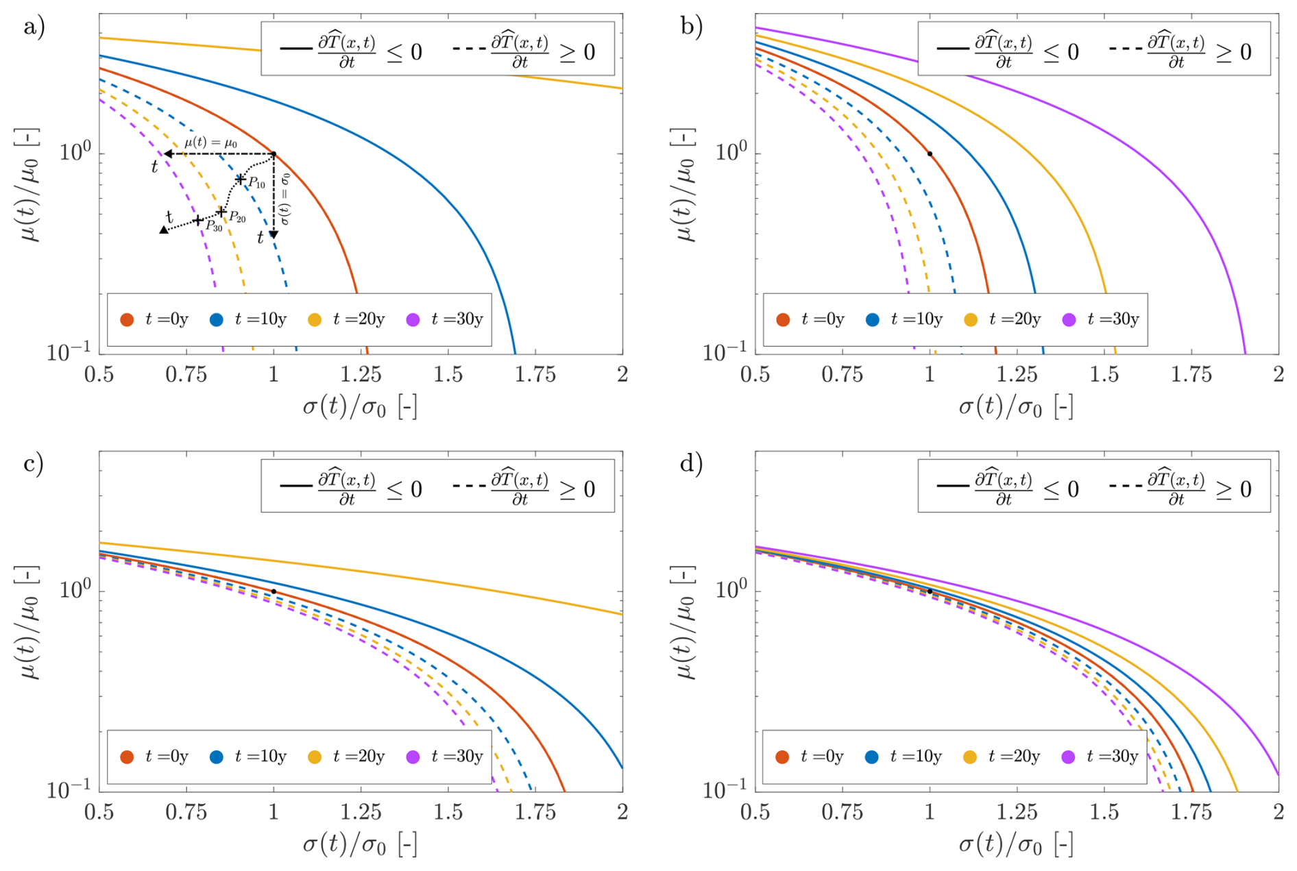
Figure 2 The graphical behavior of Eq. (13) at varying the initial return period, ${\stackrel{\mathrm{‾}}{T}}_{\mathrm{0}}\left(x\right)$, for the Fréchet (panel a and b) and the Weibull (panel c and d) distributions at different future timeframes, t, for both the cases of decreasing (solid line) and increasing (dashed line) return period. The black dot highlights the initial condition in all the panels. In panel (a), dashed-dotted black lines show time evolution for the trend in one single parameter (Eqs. 14 and 15), and the dotted black line shows a general trend in both the parameters, for the case of increasing return period. The points P_t identify the limit solution at time t along the trend line. a=1 in all the panels. (a) Fréchet distribution, ${\stackrel{\mathrm{‾}}{T}}_{\mathrm{0}}\left(x\right)$ = 25 y; (b) Fréchet distribution, ${\stackrel{\mathrm{‾}}{T}}_{\mathrm{0}}\left(x\right)$ = 50 y; (c) Weibull distribution, ${\stackrel{\mathrm{‾}}{T}}_{\mathrm{0}}\left(x\right)$ = 25 y; (d) Weibull distribution, ${\stackrel{\mathrm{‾}}{T}}_{\mathrm{0}}\left(x\right)$ = 50 y; (b) ${\stackrel{\mathrm{‾}}{T}}_{\mathrm{0}}\left(x\right)$ = 50 y. In panels (a) and (c), the continuous violet line does not satisfy the condition $t\le \frac{{\stackrel{\mathrm{‾}}{T}}_{\mathrm{0}}\left(x\right)-\mathrm{\Delta }\mathit{\tau }}{a}$, and therefore it is not shown.

In the case of the Gumbel distribution, the limit solution to Eq. (11) reads:

$$\begin{array}{}\text{(18)}& {\displaystyle \frac{{\mathit{\lambda }}_M(x,t)}{{\mathit{\lambda }}_{\mathrm{0}}}}\exp \left[-\mathrm{2}{\displaystyle \frac{x}{{\mathit{\gamma }}_M(x,t)}}\right]={\displaystyle \frac{G_{\pm }(x,t)}{G_{\mathrm{0}}\left(x\right)}}\exp \left[-\mathrm{2}{\displaystyle \frac{x}{{\mathit{\gamma }}_{\mathrm{0}}}}\right]\end{array}$$

where γ_M(x,t) and λ_M(x,t) are the maximum/minimum (plus/minus sign) values of the time-varying mean magnitude and frequency of the process, respectively, that satisfy the hypothesis of weak non-stationarity (Eq. 8), and γ₀ and λ₀ are the values of the mean magnitude and frequency, respectively, at t=0. Similarly to Eq. (13), the terms $G_{\pm }(x,t)$ and G₀ can be replaced by the expressions provided in Eqs. (11) and (12), respectively. Additionally, Eq. (18) can be further simplified when the trend affects either γ(t) or λ(t). In the first case, a solution for the limit conditions on γ_M(x,t) can be found as:

$$\begin{array}{}\text{(19)}& {\displaystyle \frac{{\mathit{\gamma }}_M(x,t)}{{\mathit{\gamma }}_{\mathrm{0}}}}={\left(\mathrm{1}+{\displaystyle \frac{{\mathit{\gamma }}_{\mathrm{0}}}{\mathrm{2}X}}\log \left[{\displaystyle \frac{G_{\mathrm{0}}\left(x\right)}{G_{\pm }(x,t)}}\right]\right)}^{-\mathrm{1}}\end{array}$$

and the limit solution for λ_M(x,t) when there is no trend on γ(t) can be retrieved as:

$$\begin{array}{}\text{(20)}& {\displaystyle \frac{{\mathit{\lambda }}_M(x,t)}{{\mathit{\lambda }}_{\mathrm{0}}}}={\displaystyle \frac{G_{\pm }(x,t)}{G_{\mathrm{0}}\left(x\right)}}\end{array}$$

Hereafter, the limit conditions are analyzed in terms of the initial return period ${\stackrel{\mathrm{‾}}{T}}_{\mathrm{0}}\left(x\right)$ (Eq. 1), and the future timeframe, t, with particular focus on the case of increasing value of the G(x,t) function (i.e., decreasing return period in non-stationary conditions). Furthermore, the approximation error for the weakly non-stationary assumption is investigated in terms of the dimensionless parameter a and in comparison to the fully non-stationary solution given by Eq. (2), as:

$$\begin{array}{}\text{(21)}& \mathrm{\Delta }\widehat{T}(x,t)={\displaystyle \frac{\widehat{T}(x,t)-\stackrel{\mathrm{̃}}{T}(x,t)}{\stackrel{\mathrm{̃}}{T}(x,t)}}\end{array}$$

3 Results

An example of the behavior of the limit solutions for the Frechét and Weibull distributions (Eq. 13) is shown in Fig. 2 for both the distributions, by varying the initial return period, ${\stackrel{\mathrm{‾}}{T}}_{\mathrm{0}}\left(x\right)$. For the sake of simplicity, we have considered a=1. Initial values of μ₀=302, σ₀=170, and ξ = ± 0.354 are taken from the application example of Salas and Obeysekera (2014).

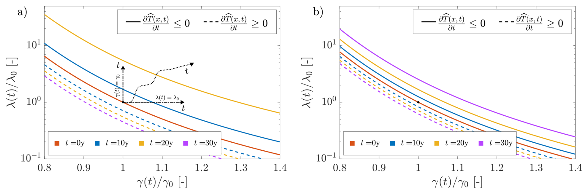
Figure 3 The graphical behavior of the limit solution for the Gumbel distribution (Eq. 18) at different future time horizons, t, for both the cases of decreasing (solid line) and increasing (dashed line) return period. The black dot highlights the initial condition in both panels (λ₀=73, γ₀=50). In panel (a), dashed-dotted black lines show time evolution for the trend in one single parameter (Eqs. 19 and 20), and the dotted black line shows a general trend in both the parameters, for the case of decreasing return period. a=1 in all the panels. The panels refer to two different values of the initial return period: (a) ${\stackrel{\mathrm{‾}}{T}}_{\mathrm{0}}\left(x\right)$ = 25 y; (b) ${\stackrel{\mathrm{‾}}{T}}_{\mathrm{0}}\left(x\right)$ = 50 y. In panels (a), the continuous violet line does not satisfy the condition $t\le \frac{{\stackrel{\mathrm{‾}}{T}}_{\mathrm{0}}\left(x\right)-\mathrm{\Delta }\mathit{\tau }}{a}$, and therefore it is not shown.

The global solution (Eq. 10) at a specific time, $\widehat{t}$, is represented by the area contained between the limit curve corresponding to the time $\widehat{t}$ and the initial curve at t=0y (orange line in Fig. 2). Therefore, any possible trend that keeps the pair of parameter values inside the aforementioned area for $t\le \widehat{t}$ satisfies the weak non-stationary hypothesis (Eq. 8). For instance, the dotted line in Fig. 2a highlights a possible general trend of the parameter μ(t) and σ(t). Considering the three limit solutions provided in the plot (at t = 10 y, at t = 20 y, and at t = 30 y), the trend satisfies the weakly non-stationary condition if the corresponding points $P_{t_{\mathrm{1}}}$ (black crosses in Fig. 2a) are reached at a time larger than, or equal to t₁. In other words, weakly non-stationary processes are represented by those pairs of parameters [σ(t),μ(t)] that change along the curvilinear axis depicting the trend slower than (or equal to) the limit solution.

The domain of allowed pairs of the process parameters strongly depends on the initial return period, ${\stackrel{\mathrm{‾}}{T}}_{\mathrm{0}}\left(x\right)$, and decreases with increasing ${\stackrel{\mathrm{‾}}{T}}_{\mathrm{0}}\left(x\right)$. As shown in the panels of Fig. 2, the distance between the limit curves is narrower in the case of greater initial return period (${\stackrel{\mathrm{‾}}{T}}_{\mathrm{0}}\left(x\right)$ = 25 y in Fig. 2a and c, and ${\stackrel{\mathrm{‾}}{T}}_{\mathrm{0}}\left(x\right)$ = 50 y in Fig. 2b and d). Similar considerations can be done when comparing the limit curves for the decreasing or increasing return periods (solid and dashed, respectively, lines in Fig. 2): in the latter case, the limit conditions on the parameters appear more restrictive. Furthermore, for the same combination of initial return period, ${\stackrel{\mathrm{‾}}{T}}_{\mathrm{0}}\left(x\right)$, and timeframe, t, Fig. 2 shows that the allowed range of validity is larger for the Fréchet distribution than for the Weibull (e.g., compare panel a and c); The behavior of the limit solutions for the Gumbel distribution is hereafter analyzed in terms of the allowed trends for the mean frequency, λ_M(x,t), and mean magnitude, γ_M(x,t), of stochastic events (Fig. 1). Figure 3 shows the behavior of the limit solution described by Eq. (18) for two different values of the initial return period, ${\stackrel{\mathrm{‾}}{T}}_{\mathrm{0}}\left(x\right)$, and for various future timeframes, t.

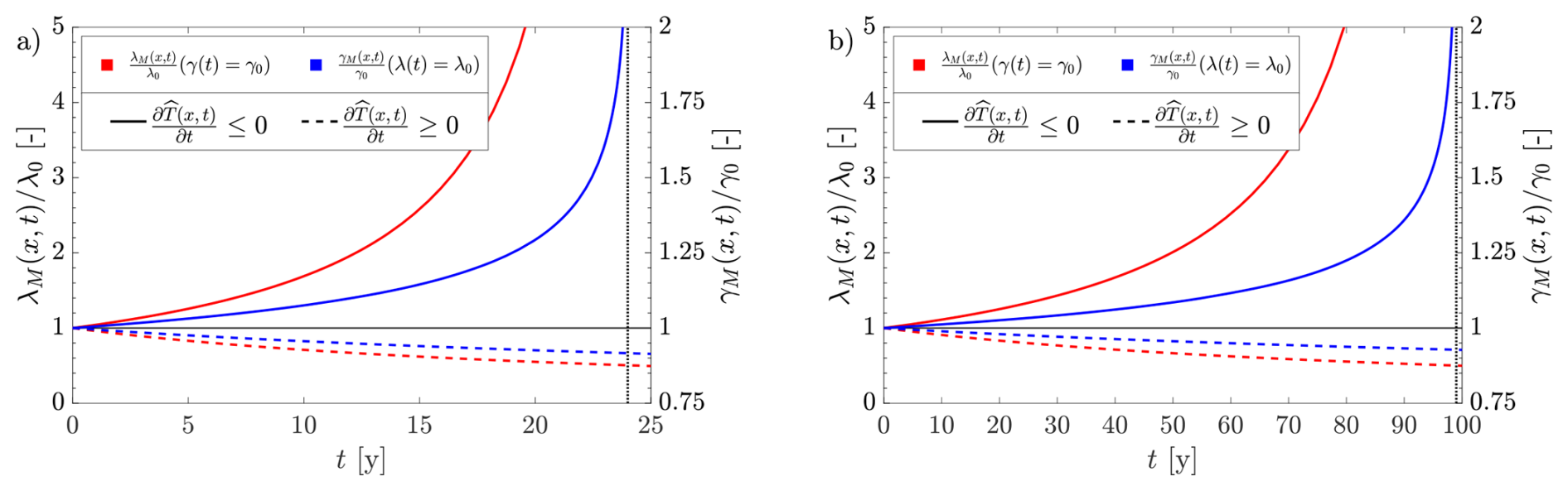
Figure 4 The simplified solution of Eqs. (20) and (19) in case the trend affects one parameter at a time. Both the solutions for decreasing (solid line) and increasing (dashed line) return period at different future timeframes, t, are shown (a=1 in both the panels). The plots refer to two different values of the initial return period: (a) ${\stackrel{\mathrm{‾}}{T}}_{\mathrm{0}}\left(x\right)$ = 25 y; (b) ${\stackrel{\mathrm{‾}}{T}}_{\mathrm{0}}\left(x\right)$ = 100 y. In both the panels, the vertical asymptote represents the limit condition $t=\frac{{\stackrel{\mathrm{‾}}{T}}_{\mathrm{0}}\left(x\right)-\mathrm{\Delta }\mathit{\tau }}{a}$, which is equal to $t={\stackrel{\mathrm{‾}}{T}}_{\mathrm{0}}\left(x\right)-\mathrm{1}$ for Δτ = 1 year and a=1.

For the tested initial return periods (${\stackrel{\mathrm{‾}}{T}}_{\mathrm{0}}\left(x\right)$ = 25 y in panel a; ${\stackrel{\mathrm{‾}}{T}}_{\mathrm{0}}\left(x\right)$ = 50 y in panel b), a reasonable variation of the parameter λ_M(t) spans two orders of magnitude, whereas the variation of the parameter γ_M(t) is limited by approximately −20 % and +40 %. The validity of the solution at a specific time horizon, t, follows the same considerations as in the case of the Fréchet and Weibull distribution (Fig. 2). Furthermore, Figs. 2a, c, and 3a show the absence of the curve at t = 30 y for the case of decreasing return period (solid line). Indeed, the proposed framework loses validity for $t\ge \frac{{\stackrel{\mathrm{‾}}{T}}_{\mathrm{0}}\left(x\right)-\mathrm{\Delta }\mathit{\tau }}{a}$ in the case of decreasing return period, due to the argument of the logarithm within the function $G_{\pm }(x,t)$ in Eq. (11). The limitation does not apply in the case of increasing return period (dashed lines in Figs. 2 and 3). In the case of the Gumbel distribution, this is highlighted in Fig. 4, where the simplified solutions (i.e., the trend affects only one parameter at a time, Eqs. 19 and 20) show the presence of an asymptote at $t={\stackrel{\mathrm{‾}}{T}}_{\mathrm{0}}\left(x\right)-\mathrm{1}$ (Δτ = 1 year and a=1 in the shown examples), for the case of decreasing return period (solid lines). The asymptote applies to the limit curves of λ_M(x,t) (solid red line) and γ_M(x,t) (solid blue line).

4 Discussion

The return period is a concept that exists theoretically for strictly stationary and ergodic time series and has been extensively used in several engineering disciplines for design and risk analysis purposes. Despite the return period concept possessing a rigorous theoretical foundation, its practical use has ever since encountered the challenging issue of dealing with observations of limited duration. This required loosening the strict assumption of stationarity and ergodicity when statistical moments and parameters are empirically calculated. Several procedures to estimate the process parameters, as well as to forecast their values in the future (i.e., trends and shifts), have been proposed in the literature (e.g., Obeysekera and Salas, 2014; Cheng et al., 2014; Villarini et al., 2009) and were therefore not the scope of this work. Herein, we assumed that the parameters of the non-stationary process and their variation in time are known based on some formulated assumptions and data fitting models (e.g., Rao, 1970; Velasco, 1999). Based on this assumption, the proposed framework has been developed to define under which statistical conditions such a time series can be assumed as weakly non-stationary. Accordingly, it allows for performing a return period analysis strictly valid within Δτ (equal to 1 year for the shown results, and in general for annual maxima analysis), by determining a condition linking the maximum change of return period in relation to the timeframe, t. We've shown that constraining the maximum change of the return period over a given timeframe, t, and quasi-stationary properties within Δτ, leads to some limits in the range of variability of the process parameters.

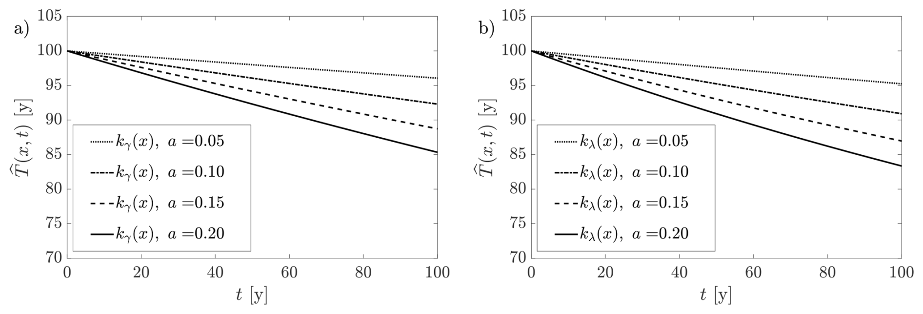
Figure 5 The value of the initial stationary return period ${\stackrel{\mathrm{‾}}{T}}_{\mathrm{0}}\left(x\right)$ = 100 y varies in time (future timeframe, t) due to a linear trend in the Gumbel distribution, for different values of the parameter a of the weakly non-stationary framework (Eq. 8). The linear trend in γ(t), k_γ, is given by Eq. (22). The linear trend in λ(t), k_λ, is given by Eq. (23). (a) Time-varying return period with a linear trend in γ(t); (b) Time-varying return period with a linear trend in λ(t).

For the simple Poisson process with marked magnitudes being considered, the limits of applicability of our analysis for the case of trends affecting either the mean frequency or the mean magnitude are shown in Fig. 4. For example, consider a process with a threshold corresponding to a present-day ${\stackrel{\mathrm{‾}}{T}}_{\mathrm{0}}\left(x\right)$ = 25 y (Fig. 4a) or ${\stackrel{\mathrm{‾}}{T}}_{\mathrm{0}}\left(x\right)$ = 100 y (Fig. 4b), and the case of decreasing return period (continuous lines in Fig. 4). Then, our analysis may be applied over a time horizon t if any trend affecting the process, either in the frequency or the magnitude, produces a change in such parameters less than the value of the corresponding curves. As said, an increase in the frequency or magnitude of events yields a reduction of $\widehat{T}(x,t)$ over that timeframe. Such a change in the mean frequency or magnitude increases with the timeframe length, ultimately reaching an infinite value at the asymptote $t=\frac{{\stackrel{\mathrm{‾}}{T}}_{\mathrm{0}}\left(x\right)-\mathrm{\Delta }\mathit{\tau }}{a}$, in the case of decreasing return period (see Fig. 5).

However, the increasing value of the limit condition is counteracted by the shorter timeframe for which the value is allowed. Specifically, if we consider the limit condition on the mean frequency parameter at a specific timeframe $\widehat{t}>\mathrm{0}$, ${\mathit{\lambda }}_M(x,\widehat{t})$, its value is valid for $\widehat{t}\le t\le \frac{{\stackrel{\mathrm{‾}}{T}}_{\mathrm{0}}\left(x\right)-\mathrm{\Delta }\mathit{\tau }}{a}$, and such a range decreases as $\widehat{t}$ increases. Similar considerations can be assessed on the parameter γ_M(x,t). Nevertheless, Fig. 4 shows that the graphs of γ_M(x,t) and λ_M(x,t) are strictly monotonic throughout the whole range of timeframe validity. Consequently, it suggests that a range of linear trends satisfying the limit condition exists for the case of a single time-varying parameter. The maximum slope of such a range is given by the derivative of the limit condition at t=0 in Fig. 4. Without losing generality of the following considerations, hereafter we focus on the case of the Gumbel distribution (ξ→0 in Eq. 3).

In this case, by considering Eqs. (19) and (20), and a linear trend in either one of the parameters in the form $A\left(t\right)=A_{\mathrm{0}}(\mathrm{1}+k_{A}t)$ with A=γ or A=λ and k_A the coefficient of the linear trend, the maximum slope can be retrieved as:

$$\begin{array}{}\text{(22)}& \begin{array}{rl}{k}_{\mathit{\gamma }}\left(x\right)& ={\displaystyle \frac{\mathrm{1}}{{\mathit{\gamma }}_{\mathrm{0}}}}{\displaystyle \frac{\partial {\mathit{\gamma }}_M(x,t)}{\partial t}}{|}_{t=\mathrm{0}}\\ & ={\displaystyle \frac{a}{{\stackrel{\mathrm{‾}}{T}}_{\mathrm{0}}\left(x\right)}}{\displaystyle \frac{\mathrm{\Delta }\mathit{\tau }}{{\stackrel{\mathrm{‾}}{T}}_{\mathrm{0}}\left(x\right)-\mathrm{\Delta }\mathit{\tau }}}{\displaystyle \frac{\mathrm{2}x}{{\mathit{\gamma }}_{\mathrm{0}}}}{\left({\displaystyle \frac{{\mathit{\gamma }}_{\mathrm{0}}}{\mathrm{2}x+{\mathit{\gamma }}_{\mathrm{0}}}}\right)}^{\mathrm{2}}\\ & \times {\left(\log \left[{\displaystyle \frac{{\stackrel{\mathrm{‾}}{T}}_{\mathrm{0}}\left(x\right)}{{\stackrel{\mathrm{‾}}{T}}_{\mathrm{0}}\left(x\right)-\mathrm{\Delta }\mathit{\tau }}}\right]\right)}^{-\mathrm{1}}\end{array}\end{array}$$

for a linear trend in the parameter γ(t) (horizontal dashed-dotted line in Fig. 3a), and

$$\begin{array}{}\text{(23)}& \begin{array}{rl}{k}_{\mathit{\lambda }}\left(x\right)& ={\displaystyle \frac{\mathrm{1}}{{\mathit{\lambda }}_{\mathrm{0}}}}{\displaystyle \frac{\partial {\mathit{\lambda }}_M(x,t)}{\partial t}}{|}_{t=\mathrm{0}}\\ & ={\displaystyle \frac{a}{{\stackrel{\mathrm{‾}}{T}}_{\mathrm{0}}\left(x\right)}}{\displaystyle \frac{\mathrm{\Delta }\mathit{\tau }}{{\stackrel{\mathrm{‾}}{T}}_{\mathrm{0}}\left(x\right)-\mathrm{\Delta }\mathit{\tau }}}{\left(\log \left[{\displaystyle \frac{{\stackrel{\mathrm{‾}}{T}}_{\mathrm{0}}\left(x\right)}{{\stackrel{\mathrm{‾}}{T}}_{\mathrm{0}}\left(x\right)-\mathrm{\Delta }\mathit{\tau }}}\right]\right)}^{-\mathrm{1}}\end{array}\end{array}$$

for a linear trend in the parameter λ(t) (vertical dashed-dotted line in Fig. 3a). For a given initial return period, ${\stackrel{\mathrm{‾}}{T}}_{\mathrm{0}}\left(x\right)$, both Eqs. (22) and (23) show that the maximum allowed linear trend mainly depends on the value of the parameter a. For such linear trends, under the hypothesis of the weakly non-stationary framework, the time variation (Eq. 5) of the initial return period ${\stackrel{\mathrm{‾}}{T}}_{\mathrm{0}}\left(x\right)$ = 100 y is shown in Fig. 5 for different values of the parameter a. For the explored range of a-values, minor differences are shown between the case with a trend in γ(t) only (Fig. 5a) and the case with a trend in λ(t) only (Fig. 5b). Particularly, the trend on the mean magnitude, γ(t), seems more restricting, as the allowed change in time is lower, compared to the case with maximum linear trend in the average frequency, λ(t).

From a practical point of view, the limit solutions for the values of the GEV parameters (Eqs. 14 and 15 for the weibull-Fréchet type, and Eqs. 19 and 20 for the Gumbel distribution) have to be compared to forecasted trends from data analysis or modelled scenarios. As an example, Fig. 6 shows this comparison for the parameter λ and a sample modelled scenario of trend with decreasing return period. Due to the uncertainty in the estimation, at each future timeframe, t, the value of the forecasted parameter, λ_F(t), is provided with a probability distribution function (light blue curves in Fig. 6) and the mean trend is represented by the continuous blue line. The shaded area of the pdf below the red curve (i.e., the limit solution) quantifies the probability that the forecasted trend satisfies the weakly non-stationary conditions in the proposed framework. In this regard, the deterministic timeframe limit of validity is defined by the point at which the forecasted trend (blue line) intersects the limit solution (red curve), i.e., t≃ 13 y in the shown example (Fig. 6). Conversely, from a probabilistic point of view, even when the average trend is above the limit solution (e.g., at t = 15 y in Fig. 6), a finite probability, although small, exists for a valid weakly non-stationary approach to the return period analysis.

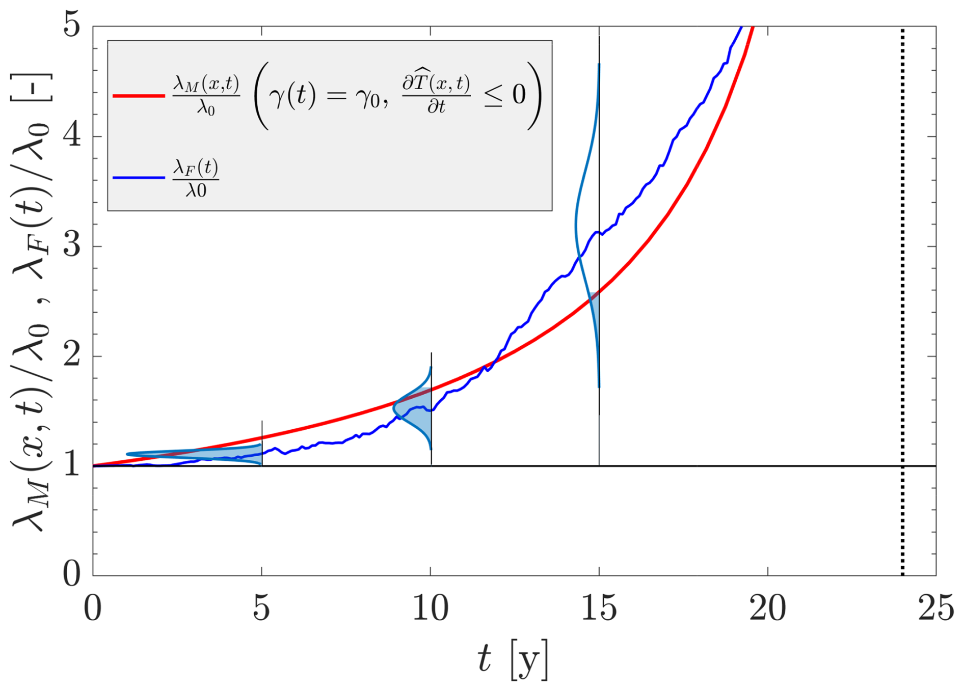
Figure 6 A comparison between the limit solution (red line) for λ_M(x,t) (Eq. 20, with a=1 and ${\stackrel{\mathrm{‾}}{T}}_{\mathrm{0}}\left(x\right)$ = 25 y) and a hypothetically-forecasted trend, λ_F (blue line), with the uncertainty estimation given by the pdf (light blue curves). At each future timeframe t, there is a probability (shaded area in each pdf) that the forecasted trend satisfies the weakly-nonstationary condition (i.e., ${\mathit{\lambda }}_{\mathrm{F}}\left(t\right)\le {\mathit{\lambda }}_M(x,t)$).

Figure 7 The degree of approximation (Eq. 21) of the proposed framework at varying the initial return period, ${\stackrel{\mathrm{‾}}{T}}_{\mathrm{0}}\left(x\right)$ and the parameter a, for the cases of linear trend in the mean magnitude (k_γ(x), Eq. 22, panel a) and mean frequency (k_λ(x), Eq. 23, panel b).

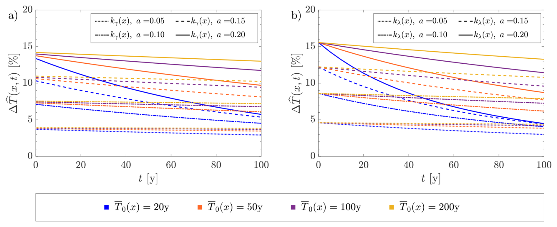
The approximation error of the proposed weakly non-stationary framework is evaluated through Eq. (21) for different combinations of initial stationary return period ${\stackrel{\mathrm{‾}}{T}}_{\mathrm{0}}\left(x\right)$, a-parameter, and the corresponding maximum linear trend in either γ(t) or λ(t). As expected from Eq. (8), Fig. 7 shows that the greater the allowed change in time of the return period (i.e., the a parameter), the greater the approximation error $\mathrm{\Delta }\widehat{T}(x,t)$. Following the considerations on the maximum allowed value of the linear trend (k_γ and k_λ in Fig. 5), $\mathrm{\Delta }\widehat{T}(x,t)$ is greater when the trend affects the mean frequency λ(t) (Fig. 7b) than the mean magnitude γ(t) (Fig. 7a), for the same combination of a and ${\stackrel{\mathrm{‾}}{T}}_{\mathrm{0}}\left(x\right)$. Furthermore, the approximation error decreases according to the timeframe t, and maximizes at the current time (t = 0 y). This is because Eq. (2) accounts for the future time-varying values of the GEV distribution, whereas the proposed framework considers the local (in time) values. Therefore, the weakly non-stationary return period at t=0, $\widehat{T}(x,\mathrm{0})$ is equal to the initial return period, ${\stackrel{\mathrm{‾}}{T}}_{\mathrm{0}}\left(x\right)$, under stationary conditions. By considering the best tested combination (corresponding to a=0.05), Fig. 7 shows that the approximation error is roughly in the order of 5 % for all the tested initial return periods, and this is achieved by one single calculation (Eq. 5) for all the future timeframes, t. Conversely, Eq. (2) requires the computation of infinite terms, and the operation should be repeated for all the timeframes. An approximate solution of the fully non-linear return period, $\stackrel{\mathrm{̃}}{T}(x,t)$ can be assessed by considering only the first N terms in the summation of Eq. (2). In this case, the degree of approximation of the calculated value, ${\stackrel{\mathrm{̃}}{T}}_{\mathrm{0},N}\left(x\right)$, depends on the number of terms, N, on the threshold X (i.e., the value of the associated stationary return period $\stackrel{\mathrm{‾}}{T}\left(x\right)$, and the effective trend in the process signal.

To give an example, Fig. 8 shows the degree of approximation of the solution with N terms in the summation, and the actual return period under non-stationary conditions using Eq. (2), for a Poisson Process (Fig. 1a) with initial mean frequency λ₀ = 73 y⁻¹, and a linear trend in the mean frequency depending on the coefficient k_λ, in the form $\mathit{\lambda }\left(t\right)={\mathit{\lambda }}_{\mathrm{0}}(\mathrm{1}+k_{\mathit{\lambda }}t)$. Fig. 8 suggests that an approximated solution with few terms (N≤100) of Eq. (2) is reliable only in the case of a low initial return period and high trends in the process signal (e.g., ${\stackrel{\mathrm{‾}}{T}}_{\mathrm{0}}\left(x\right)$ = 20 y and k_λ = 0.01 y⁻¹, dashed blue line in Fig. 8). Conversely, for higher return periods (e.g., ${\stackrel{\mathrm{‾}}{T}}_{\mathrm{0}}\left(x\right)\ge$ 50 y) and milder trends (k_λ≤ 0.01 y⁻¹), the required number of terms to get a good approximation of the return period in non-stationary conditions increases by an order of magnitude, in the shown example. For instance, in the case of ${\stackrel{\mathrm{‾}}{T}}_{\mathrm{0}}\left(x\right)$ = 200 y and k_λ = 10⁻⁴ y⁻¹ 500 terms lead to get an approximated value equal to 73 % of the actual one, whereas 1000 terms are necessary to obtain an approximation of 97 % (dotted yellow line in Fig. 8).

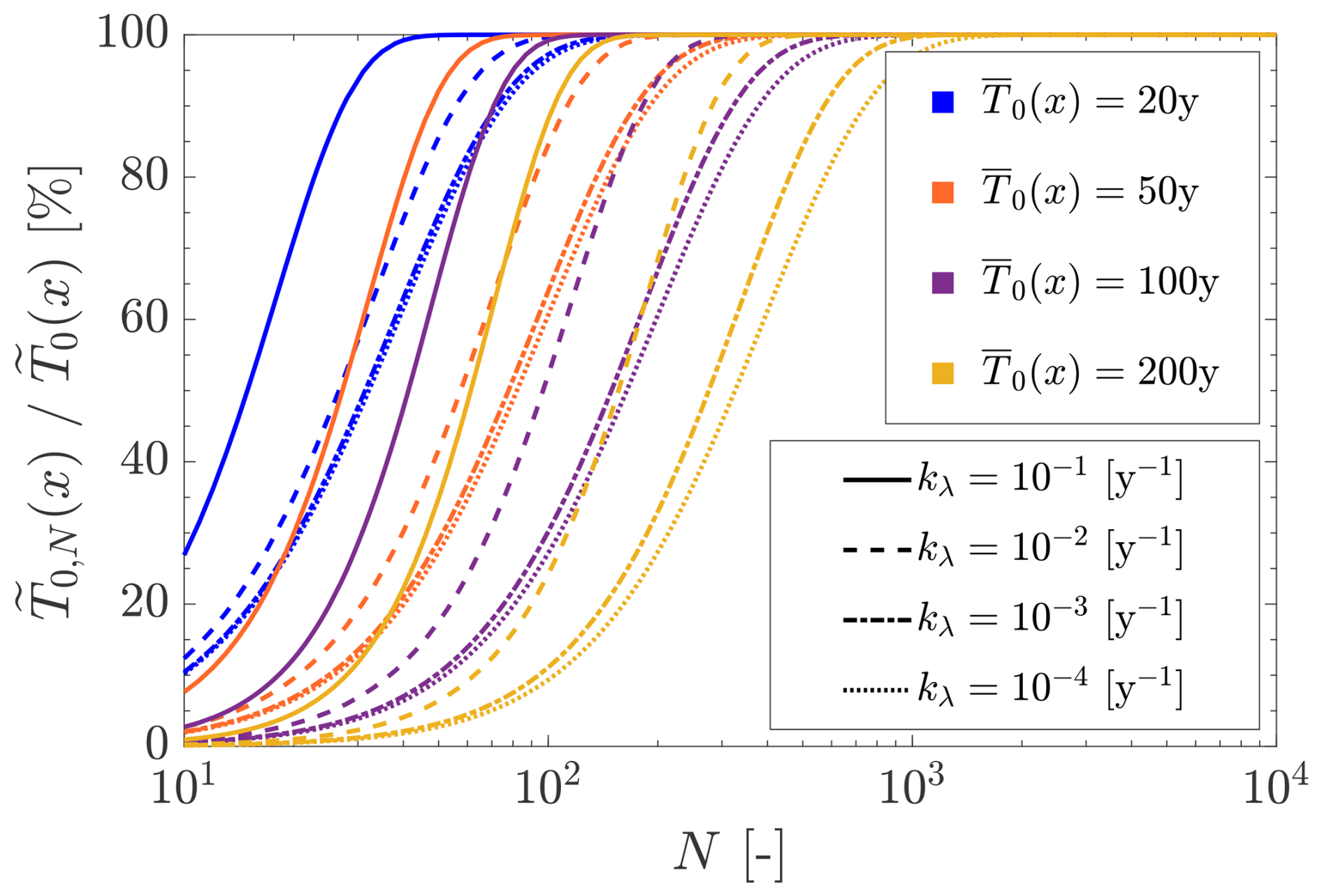
Figure 8 A comparison between the approximated solution of Eq. (2) with N terms, ${\stackrel{\mathrm{̃}}{T}}_{\mathrm{0},N}\left(x\right)$, and the actual solution, ${\stackrel{\mathrm{̃}}{T}}_{\mathrm{0}}\left(x\right)$, according to different combinations of initial stationary return period, ${\stackrel{\mathrm{‾}}{T}}_{\mathrm{0}}\left(x\right)$, and linear trend coefficient in the mean frequency, k_λ, of a Poisson Process with initial mean frequency, λ₀ = 73 y⁻¹.

5 Conclusions

A novel framework for the return period analysis of non-stationary time series is proposed. The model is based on the hypothesis of weak non-stationarity, by assuming that the changes in the governing parameters (presence of trends) occur on a timescale longer than that of the change of statistical characteristics of the process (e.g., return period). Closed-form solutions are derived for the maximum allowed trends for the General Extreme Value distribution, and specifically discussed in the case of a linear trend for the Gumbel distribution. As a result, once the GEV parameters are known from fitting models or forecasted scenarios, the maximum timeframe for the validity of the weakly non-stationarity analysis can be retrieved in the case of decreasing return period for specific values of the parameter a, which in turn drives the estimation error (e.g., Fig. 7). The results are readily applicable, but not limited, to the design of hydraulic structures, for which the return period and its time-varying value may affect the failure statistics.

Appendix A: General equation for GEV parameters of weakly non-stationary processes

Based on Eq. (8), a relationship on the parameters governing the limit time-evolution of the GEV distribution under the hypothesis of weakly non-stationary processes can be derived by accounting for the original definition of the GEV function (Eq. 3). The relationship reads:

$$\begin{array}{}\text{(A1)}& \begin{array}{rl}& \left|{\displaystyle \frac{\begin{array}{c}\frac{{\mathit{\xi }}^{\prime }\left(t\right)}{\mathit{\xi }\left(t\right)}\left(\frac{\mathrm{1}}{\mathit{\xi }\left(t\right)}+\frac{x-\mathit{\mu }\left(t\right)}{\mathit{\sigma }\left(t\right)}\right)\log \left[\mathrm{1}+\mathit{\xi }\left(t\right)\frac{x-\mathit{\mu }\left(t\right)}{\mathit{\sigma }\left(t\right)}\right]\\ +\left(\frac{{\mathit{\sigma }}^{\prime }\left(t\right)}{\mathit{\sigma }\left(t\right)}-\frac{{\mathit{\xi }}^{\prime }\left(t\right)}{\mathit{\xi }\left(t\right)}\right)\frac{x-\mathit{\mu }\left(t\right)}{\mathit{\sigma }\left(t\right)}+\frac{{\mathit{\mu }}^{\prime }\left(t\right)}{\mathit{\sigma }\left(t\right)}\end{array}}{{\left(\mathrm{1}+\mathit{\xi }\left(t\right)\frac{x-\mathit{\mu }\left(t\right)}{\mathit{\sigma }\left(t\right)}\right)}^{\frac{\mathit{\xi }\left(t\right)+\mathrm{1}}{\mathit{\xi }\left(t\right)}}}}\right|\\ \le & {\displaystyle \frac{a}{\mathrm{\Delta }\mathit{\tau }}}{\displaystyle \frac{(\mathrm{1}-\mathrm{GEV}(x,t){)}^{\mathrm{2}}}{\mathrm{GEV}(x,t)}}\end{array}\end{array}$$

where the prime ^′ notation stands for the derivative with respect to time (e.g., ${\mathit{\xi }}^{\prime }\left(t\right)=\mathrm{d}\mathit{\xi }\left(t\right)/\mathrm{d}t$). Equation (A1) represents the most general solution to the definition of weakly non-stationary processes and their return period analysis in terms of the process parameters (i.e., ξ(t), μ(t), and σ(t)). Its solution is anything but straightforward, and some simplifying assumptions should be considered for its mathematical tractability. For instance, considering that the shape parameter, ξ(t), remains constant (i.e., ξ(t)=ξ), Eq. (A1) can be simplified into:

$$\begin{array}{}\text{(A2)}& \begin{array}{rl}& \left|{\displaystyle \frac{{\mathit{\sigma }}^{\prime }\left(t\right)\frac{x-\mathit{\mu }\left(t\right)}{\mathit{\sigma }\left(t\right)}+{\mathit{\mu }}^{\prime }\left(t\right)}{\mathit{\sigma }\left(t\right){\left(\mathrm{1}+\mathit{\xi }\frac{x-\mathit{\mu }\left(t\right)}{\mathit{\sigma }\left(t\right)}\right)}^{\frac{\mathit{\xi }+\mathrm{1}}{\mathit{\xi }}}}}\right|\\ \le & {\displaystyle \frac{a}{\mathrm{\Delta }\mathit{\tau }}}{\displaystyle \frac{(\mathrm{1}-\mathrm{GEV}(x,t){)}^{\mathrm{2}}}{\mathrm{GEV}(x,t)}}{|}_{\mathit{\xi }\left(t\right)=\mathit{\xi }}\end{array}\end{array}$$

From Eq. (A2), the structure of the GEV distribution should be imposed, thus leading to the analysis carried out in the Methods section.