Estimating robust melt factors and temperature thresholds for snow modelling across the Northern Hemisphere

Hydrological models commonly use very simple snow accumulation and melt models based on air temperature information, namely, a temperature threshold for snow accumulation as well as for snowmelt, and a melt factor. This utility emerges due to the simplicity, efficiency, and generally good performance of such models if sufficient calibration information is available. At scales beyond single gauged catchments, the estimation and evaluation of the temperature thresholds and the melt factor has been difficult due to a lack of observations on snow accumulation and melt. Using a recently published Northern Hemisphere snow water equivalent dataset (NH-SWE) and co-located climate station observations of temperature and precipitation (4736 stations across the Northern Hemisphere), this work estimates melt factors and temperature thresholds for snow modelling based on station observations and provides the first large-scale and long-term (1950–2023) evaluation of a simple temperature-index snow model and its parameters across a diverse range of snow climates. Our study reveals that the 0 °C as precipitation-phase threshold captures most snowfall days (89 %) and the 0 °C as snowmelt initiation threshold captures most snowmelt days (76 %). Adjusting large-scale uniform threshold values does not consistently improve performance across all snow accumulation and melt metrics. Estimated melt factors based on observations converge towards 3–5 mm (°C d)⁻¹ for deeper snowpack climates (peak snow water equivalent >300 mm), but their estimation may be more challenging for colder climates with shallower snowpacks (<300 mm), conditions where the derived melt factors cover a wider range (1 to 12 mm (°C d)⁻¹) and a much higher interannual and spatial variability. The temperature-index snow model performs consistently well, on average, across the available Northern Hemisphere data set for estimating long-term mean values of seasonal snow cover onset, snowmelt season onset, mean snow accumulation and snowmelt rates, but challenges may arise due to biases in temperature records or solid precipitation undercatch. Peak snow water equivalent is likely underestimated for deep or alpine snowpacks, while it is likely overestimated for shallow snowpacks in the coldest and continental climates. The best median performance of the temperature-index approach lies on relatively shallow snowpacks in temperate climates. This study provides valuable insights into temperature-threshold snowfall modelling and temperature-index melt modelling for applications across diverse climates and environments, and the results should help refine regional modelling approaches to enhance our understanding of snowpack responses to global warming.

1 Introduction

The sensitivity of snow accumulation and melt to warming temperatures is crucial for predicting global hydrological responses to climate change (Nijssen et al., 2001; Barnett et al., 2005; López-Moreno et al., 2020). Our understanding of snowpack sensitivity to rising temperatures can be improved by analysing trends in historical observations of snowpacks and climate variables from in-situ measurements (Fontrodona Bach et al., 2018; Luomaranta et al., 2019; Matiu et al., 2021) or from remote sensing (Bormann et al., 2018; Notarnicola, 2022), but these may be limited in time and space. Alternatively, spatio-temporal snowpack dynamics can be analysed by simulating the response of snow accumulation and snowmelt under warming scenarios using models (Pomeroy et al., 2015; López-Moreno et al., 2021). However, model simulations are challenged by various sources of uncertainty (Oreskes et al., 1994), which may arise from natural variability (Willibald et al., 2020), parameter uncertainty (Günther et al., 2020), forcing data uncertainty (Günther et al., 2019; Terzago et al., 2020), the ability of models to represent certain processes (Cho et al., 2022), the choice of model configurations (Essery et al., 2013), or even subjective modelling decisions (Melsen et al., 2019). Two crucial aspects to model development and model applications are the reliable formulation of assumptions, the reliable estimation of model parameters and the evaluation of model simulations against actual observations.

In the case of snow accumulation modelling, accurate estimation of the rainfall-snowfall partitioning is crucial (Behrangi et al., 2018). In alpine climates, most snowfall events occur below 0 °C (Rohrer and Braun, 1994), but the actual zero degree isotherm may lie 300–400 m above the elevation at which snow starts to accumulate at the surface (Fabry and Zawadzki, 1995). Rain-snow partitioning is often better captured by the wet-bulb temperature, which depends on relative humidity and surface pressure (Jennings et al., 2018b). Inclusion of wet-bulb temperature to estimate the rain-snow partitioning has shown improved snow and streamflow simulations (Tobin et al., 2012; Zhang et al., 2015; Harpold et al., 2017; Jennings and Molotch, 2019; Wang et al., 2019), but these meteorological measurements generally have far lower availability than (dry bulb) air temperature. In practice, most contemporary studies derive the rainfall-snowfall threshold from precipitation phase observations or set it to some generally accepted value, which may differ from 0 °C. A rainfall-snowfall separation temperature range between 0 and 2 °C is often used for hydrological modelling over mountain areas (Tobin et al., 2012; Bormann et al., 2014). A wide range of studies use a fixed threshold of 0 or 1 °C even for large-scale applications (Berghuijs et al., 2014; Follum et al., 2019; Hou et al., 2023; Bonsoms et al., 2024), even though the rain-snow phase transition is more gradual and the use of a smooth threshold might be more appropriate (Dai, 2008; Jennings et al., 2025).

There are two main approaches to modelling snowmelt, (1) solving the full energy balance, or (2) using simpler approaches that relate snowmelt directly to more readily available climate variables such as temperature and incoming radiation. The first approach is physics-based, more complex, and can resolve multiple layer snowpack processes (e.g. wind redistribution, snowpack temperature gradients, sublimation, liquid water content in the snowpack). However, it is computationally expensive and requires much more meteorological forcing data (e.g. relative humidity, wind speed, incoming and outgoing shortwave and longwave radiation, and often information on the snowpack itself) (Bartelt and Lehning, 2002; Lehning et al., 2002a, b; Magnusson et al., 2017). Although such models may be more easily transferable and rely less on calibration, some physical parameters may not be well constrained and thus introduce considerable uncertainty in model simulations (Günther et al., 2020). Furthermore, applying this approach at large spatial scales, beyond hillslopes or small catchments, comes with a reduction in forcing data resolution and, therefore a reduction in model reliability and performance (Magnusson et al., 2019).

Contrasting with the requirements of physics-based models, the simplest temperature-index snowmelt model (Lang and Braun, 1990; Rango and Martinec, 1995; Hock, 2003) needs only air temperature data as forcing to simulate snowmelt. However, simplicity comes at the expense of not resolving snowpack processes other than accumulation and melt. This approach relies on the key assumption that snowmelt can be directly related to air temperature, which generally holds well (Ohmura, 2001; Sicart et al., 2006). The melt factor (with units mm (°C d)⁻¹), is a parameter that captures how much melt is produced per degree of air temperature beyond a snowmelt temperature threshold. The melt factor has to be calibrated or assumed, and the temperature threshold above which snowmelt occurs can also be calibrated (Hock, 2003), but is often assumed between −1 and 1 °C (Senese et al., 2014; Avanzi et al., 2022; Elias Chereque et al., 2024).

The interpretation and meaning of the melt factor are not trivial and fundamentally depend on the time and spatial scale over which they are estimated. Hock (2003) provides a comprehensive analysis of the variability of the melt factor and its physical basis. Generally, low melt factors indicate a low incoming shortwave radiation, a high albedo, a higher portion of melt driven by the sensible heat flux, or a combination of those. In these conditions, snowmelt is less sensitive to a change in temperature (i.e. there is not much melt per degree of temperature), and therefore the melt factor is low. Conversely, high melt factors indicate a higher incoming shortwave radiation driving a larger part of the energy balance, which causes more snowmelt than what the relationship between melt and temperature alone can explain, and therefore the melt factor is high (Hock, 2003). The daily and seasonal variation of the melt factor with incoming shortwave radiation (Ismail et al., 2023) has motivated efforts to include shortwave radiation parameterisations of the melt factor (Pellicciotti et al., 2005; Magnusson et al., 2014), but this adds complexity to the model. The melt factor also varies significantly spatially, across hydroclimatic regions, across land use or as a function of slope, aspect or sky view angles (Marsh et al., 2012). Reported melt factors for snow in the literature range between 0.5 and 20 mm (°C d)⁻¹ across many different locations, but typical values range between 2 and 6 mm (°C d)⁻¹ (Braithwaite, 1995; Kane et al., 1997; Lefebre et al., 2002; Hock, 2003; Braithwaite, 2008; Shea et al., 2009; Asaoka and Kominami, 2013).

Despite the superiority of state-of-the-art mechanistic snow models in resolving snowpack processes, temperature-index models remain widely used for large-scale snow modelling due to their computational efficiency and ability to operate at high spatial resolutions (Rittger et al., 2016; Avanzi et al., 2023; Marty et al., 2025). This is relevant to better capture the high spatial variability of snow on the ground (López-Moreno et al., 2013, 2015), which is less well captured by Hemispheric-scale coarser gridded snow datasets (Mudryk et al., 2015). However, the temperature thresholds for rain-snow partitioning and for snowmelt initiation, and the melt factors used in temperature-index models are frequently either assumed, spatially upscaled from limited point-scale observations, or calibrated at the catchment scale (Schaefli et al., 2005; Bogacki and Ismail, 2016; Riboust et al., 2019), without systematically evaluating how transferable these assumptions and parameterisations are across different climates. In particular, the melt factor has been estimated at a range of scales, from the the point, to catchment and glacier scales (Braithwaite, 1995; Lefebre et al., 2002; Shea et al., 2009; Ismail et al., 2023), but its spatial variability and performance across climates remain poorly constrained.

Given the widespread application and utility of temperature-index models, there is a need for a comprehensive assessment of temperature-index model assumptions, parameterisations, and performance across a wide range of snow climates, to better understand the environmental conditions where these models are suitable and where they may fail. The availability of recently published station-based snow water equivalent (SWE) time series over the Northern Hemisphere, NH-SWE (Fontrodona-Bach et al., 2023a, b), and co-located climate station observations of temperature and precipitation, provides the possibility to gain insights into the global variability of temperature-index melt model parameterisations, and offers the opportunity to test whether a temperature-index model can be robustly used across diverse snow climates. Where feasible, however, full energy balance modelling should be used, especially because of its more reliable transferability across climates. Because of its simplicity, the temperature-index approach can only resolve accumulation and melt (Hock, 2003), but not sublimation, snowpack water holding capacity, liquid water refreezing and melt water flow routes. However, the temperature-index approach can be combined with algorithms to account for snow redistribution (Freudiger et al., 2017).

Here, we use ground-based (station) observations of temperature and precipitation together with the NH-SWE time series to empirically derive and estimate the three key temperature-index model parameters of the classical degree-day model (the snowfall threshold, the snowmelt threshold, and the melt factor) across the Northern Hemisphere. We then use the temperature-index model to simulate SWE time series using these point-scale observations of temperature and precipitation and evaluate the model’s performance against the NH-SWE time series.

In this study, we conduct the first hemisphere-scale assessment of the classical temperature-index model across 4736 observation sites. Our analysis provides several novel contributions: (1) a large-scale and long-term evaluation and sensitivity analysis of key model assumptions – such as melt factors and temperature thresholds – and their spatial variability; (2) a transparent assessment of model strengths and limitations across environmental gradients; (3) a cross-climatic evaluation of temperature-index model performance under diverse snowpack regimes; and (4) spatial analyses that reveal systematic patterns in model performance linked to snow climate characteristics.

2 Data

2.1 Temperature and precipitation data

We use daily time series of precipitation and temperature from the global historical climatology network dataset (GHCNd, version 3.30-upd-2023080717) (Menne et al., 2012). Because of known biases in the temperature data within the SNOwpack TELemetry Network (SNOTEL) dataset (Avanzi et al., 2014; Oyler et al., 2015), which is part of GHCNd, we replace the SNOTEL data in GHCNd with the Bias Corrected and Quality Controlled (BCQC) SNOTEL Data (Yan et al., 2018; Sun et al., 2019). For better coverage of the European continent, including the European Alps, we also use time series from the European Climate Assessment and Dataset (ECA&D, https://www.ecad.eu/ last access: 3 July 2023) (Klein Tank et al., 2002), and from the MeteoSwiss data portal IDAWEB https://opendata.swiss/ (last access: 17 August 2023) (MeteoSwiss, 2023). If the mean daily temperature is unavailable, we use the daily minimum and maximum to compute the daily mean as the midpoint between the two. A total of 34 536 stations are initially available. We apply a simple gap-filling and quality control procedure (see Supplement Sect. S1) and select stations with at least 5 years of gap-free data from 1950 to 2023, although the period available does not need to be continuous. A total of 14 881 stations with temperature and precipitation time series are still available after these filters are applied.

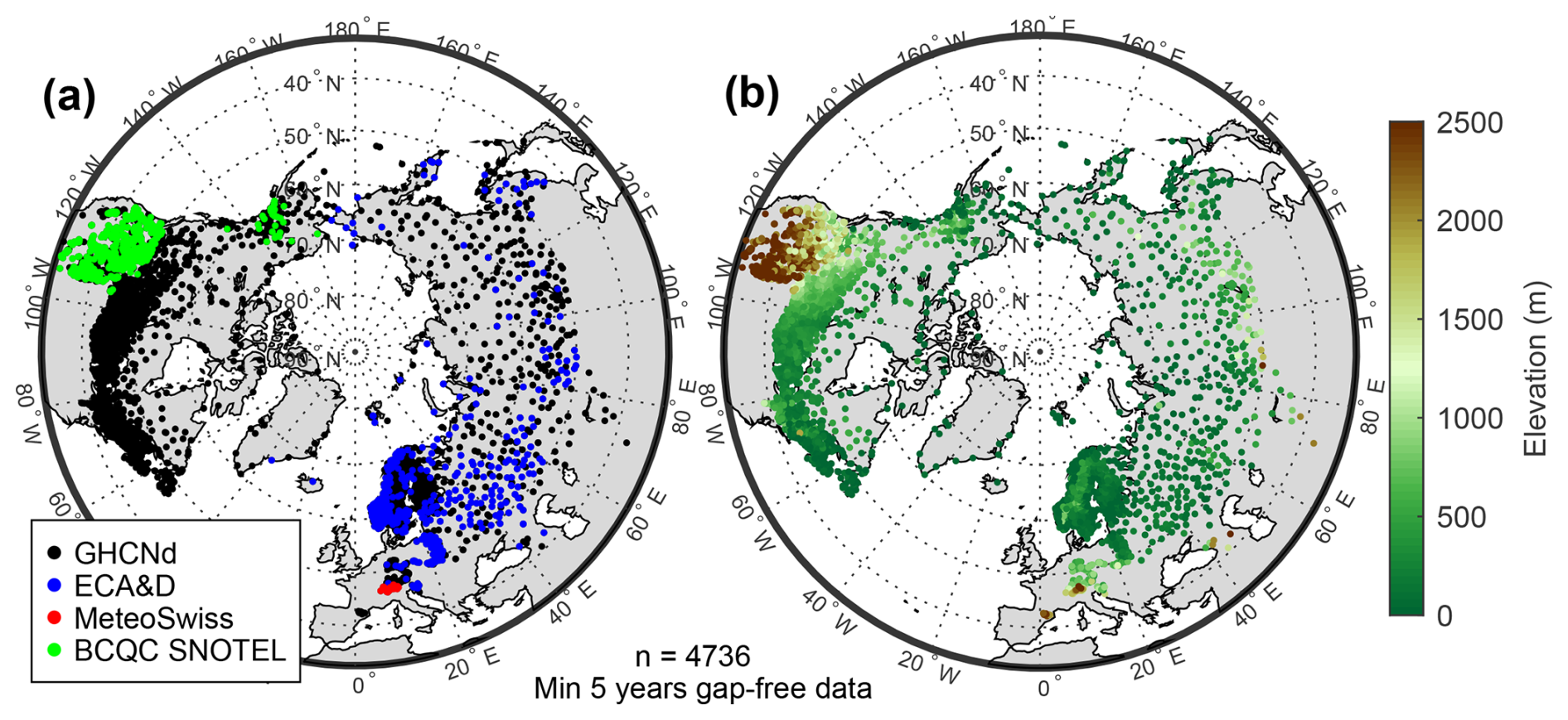
Figure 1 Matched NH-SWE stations with GHCNd/ECA&D/MeteoSwiss/BCQC-SNOTEL stations, and their elevation.

2.2 Snow water equivalent data

We use the Northern Hemisphere daily snow water equivalent time series from the NH-SWE dataset (Fontrodona-Bach et al., 2023b, a). A total of 11 071 quality-controlled and gap-filled stations are initially available in the dataset. We match the locations of the stations in the NH-SWE dataset with the locations of the stations with temperature and precipitation time series. We select those that are separated by less than 0.01° latitude and 0.01° longitude (ca. 1 km distance) from each other, with an elevation difference not larger than 10 m, and which contain at least 5 years of overlapping gap-free data with the temperature and precipitation time series. A total of 4736 stations from the NH-SWE dataset are matched with 3349 stations from the GHCNd, 766 from the BCQC SNOTEL, 593 stations from ECA&D, and 28 stations from MeteoSwiss (Fig. 1). This results in a large range of stations across elevation, latitude and longitude gradients in the Northern Hemisphere (Fig. 1). As the NH-SWE data contains only stations with at least 40 d of continuous snow cover on average, warmer climates and ephemeral snow climates are generally not included. The length of the remaining time series available shows the long-term nature of this study, with 50 % of stations having at least 30 years of available data (Fig. S1 in the Supplement).

Our study adopts the spatial scale of the Northern Hemisphere despite key data gaps in highly snow-dominated areas such as High Mountain Asia, including the Tibetan Plateau (Gao et al., 2012), Himalayas (Immerzeel et al., 2010), and high mountains in Central Asia (Gao et al., 2017), because we did not find data meeting the requirements of our study in these regions.

3 Methods

3.1 Snow season and climate indices

We use the same snow season definitions as Fontrodona-Bach et al. (2023b), as well as two temperature-based indices from Woods (2009) to define the characteristic climate of each station, and two more climate indices based on temperature and precipitation (Table 1).

Table 1 Definitions of snow season and climate indices used in this study. “dosy”: day of snow year, starting on 1 September.

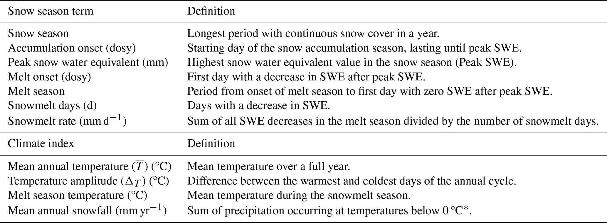
^* This threshold is later varied for the temperature-index modelling but is kept constant here to obtain a mean snowfall climatology of a station.

3.2 Temperature-index model

We simulate daily time series of snow water equivalent, SWE, using the daily time series of temperature and precipitation and a simple temperature-index model as follows:

$$\begin{array}{}\text{(1)}& {\displaystyle \frac{\mathrm{d}{H}_{\mathrm{SWE}}\left(t\right)}{\mathrm{d}t}}=A\left(t\right)-M\left(t\right),\end{array}$$

where H_SWE(t) [mm] stands for SWE at time step t [d], A(t) [mm d⁻¹] is the snow accumulation rate at time step t and M(t) [mm d⁻¹] is the snowmelt rate at time step t. We use an explicit time-stepping scheme to solve Eq. (1), i.e.:

$$\begin{array}{}\text{(2)}& H_{\mathrm{SWE},t}=H_{\mathrm{SWE},t-\mathrm{1}}+\mathrm{\Delta }(A_{t-\mathrm{1}}+M_{t-\mathrm{1}}),\end{array}$$

where Δ [d] is the time step length (in this study, daily), A_t−1 is the snow accumulation rate during time step t−1 [mm d⁻¹] and M_t−1 the snowmelt rate [mm d⁻¹] during the preceding day t−1. A_t is computed as follows:

$$\begin{array}{}\text{(3)}& A_t=\left\{\begin{array}{ll}{P}_t& \text{if}{T}_t\le T_{\mathrm{a}}\\ \mathrm{0}& \text{if}{T}_t>T_{\mathrm{a}}\end{array}\right.\end{array}$$

where P_t [mm d⁻¹] is the daily precipitation, T_a [°C] is the threshold temperature for snow accumulation, and T_t [°C] is the temperature on day t. M_t is computed as follows:

$$\begin{array}{}\text{(4)}& M_t=\left\{\begin{array}{ll}\mathit{\alpha }\times (T_t-T_{\mathrm{m}})& \text{if }{T}_t\ge T_{\mathrm{m}}\\ \mathrm{0}& \text{if }{T}_t<T_{\mathrm{m}}\end{array}\right.\end{array}$$

where α [mm (°C d)⁻¹] is the melt factor, which we assume to be constant in time, and T_m [°C] is the threshold temperature for snowmelt. Snowmelt M_t cannot exceed available snow, i.e. $\mathrm{\Delta }{M}_t\le H_{\mathrm{SWE},t}+\mathrm{\Delta }{A}_t$.

3.3 Deriving and estimating temperature-index model parameters

We empirically derive and then estimate values for two parameters of the temperature-index model for all stations in our study: the snow accumulation temperature threshold (T_a) and the melt factor (α). We also evaluate whether a T_m=0 °C threshold is a reasonable assumption for the snowmelt temperature threshold. We estimate all parameters by comparing the station-based SWE time series with co-located time series of observed temperature and precipitation.

As the SWE time series from the NH-SWE dataset are based on snow depth observations (not on direct observations of snow water content), a daily increase in SWE (ΔSWE>0) can be attributed to actual snow accumulation with high confidence (i.e. incoming snowfall exceeding any potential melt during that time step), except in rare cases of measurement noise, which are negligible at the scale of this study. We can, therefore, empirically derive the snow accumulation temperature threshold by analysing the distribution of observed daily temperatures on days with ΔSWE>0. We set, for each station, the snow accumulation temperature threshold equal to the 80th percentile of the distribution of observed temperatures on days with ΔSWE>0 (i.e., 80 % of snow accumulation days occur at or below this temperature threshold). This choice is a compromise between capturing the majority of snow accumulation events while avoiding excessive near-freezing precipitation to be classified as snow. Based on these snow accumulation thresholds empirically derived from observed data for each station, we build a simple a multilinear regression model via Ordinary Least Squares that estimates the snow accumulation threshold (T_a,e) based on the climate variables from Table 1 ($\stackrel{\mathrm{‾}}{T}$ and Δ_T). The parameter estimation model yields a coefficient of determination of R²=0.68 and the following coefficients:

$$\begin{array}{}\text{(5)}& T_{\mathrm{a},\mathrm{e}}=\mathrm{0.210}\times \stackrel{\mathrm{‾}}{T}-\mathrm{0.319}\times {\mathrm{\Delta }}_T+\mathrm{1.834}\end{array}$$

where $\stackrel{\mathrm{‾}}{T}$ is the mean annual temperature of a station, and Δ_T is the amplitude of the annual temperature cycle at a station (Table 1). However, we set the minimum threshold value to 0 °C, as the model estimates snow accumulation thresholds below 0 °C for the colder climates, which could classify too much snow as rain. We use the empirically derived and estimated parameters at each station to run the temperature-index model simulations in Sect. 3.4.

Unlike for snow accumulation, the NH-SWE time series cannot confidently distinguish whether a daily decrease in SWE (ΔSWE<0) is due to snowmelt or due to an alternative loss mechanism such as sublimation or snow redistribution by wind, or due to a model inaccuracy if the maximum snow density parameter is reached too quickly (Winkler et al., 2021; Fontrodona-Bach et al., 2023b). The minimum temperature at which ΔSWE<0 occurs cannot reliably indicate a melt threshold, as the decrease in SWE at that temperature may not be due to snowmelt but to other processes. Nevertheless, analysing the distribution of observed temperatures on days with ΔSWE<0 allows us to evaluate whether a T_m=0 °C is a reasonable assumption, and is also useful to gain insights into temperature-index modelling limitations as well as NH-SWE data limitations (see Sect. 4.1.2).

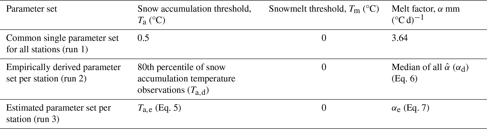
Table 2 Parameter values used for the three sets of temperature-index model simulations.

To empirically derive the daily melt factor ($\widehat{\mathit{\alpha }}$, in mm (°C d)⁻¹, from the NH-SWE time series, we divide the daily absolute magnitude of ΔSWE<0 by the corresponding observed daily temperature:

$$\begin{array}{}\text{(6)}& \widehat{\mathit{\alpha }}={\displaystyle \frac{\left|\mathrm{\Delta }\right(H_{\mathrm{SWE},t}-H_{\mathrm{SWE},t-\mathrm{1}}\left)\right|}{T_t}}\end{array}$$

Two observations are important here: (1) computed daily melt factors can become very large, or even infinite, if daily SWE decrease is small or temperature is close to zero. (2) computed melt factors can become negative (physically not possible) if ΔSWE<0 occurs on days with negative temperatures. We, therefore, remove daily melt factor values higher than 20 mm (°C d)⁻¹ (4 % of all data), as these are rare in the literature (Asaoka and Kominami, 2013), and we also remove negative values (23 % of all data). After removing these values, we define the annual melt factor as the median of all daily melt factors in a year, and the melt season melt factor as the median of daily melt factors during the snowmelt season only (as defined in Table 1). At each site, one final empirically derived melt factor (α_d) is obtained by computing the median of seasonal melt factors.

Given the variability of the melt factor with different sources of snowmelt energy, it is interesting to check whether a multilinear regression model can be used to estimate the melt factor (α_e) based on climate and geographic variables. Among the variables tested ($\stackrel{\mathrm{‾}}{T}$, Δ_T, mean annual snowfall, latitude and elevation) and following a stepwise linear regression, the best model discarded Δ_T (Table 1) as a predictor for the melt factor and shows, however, a very low coefficient of determination, R²=0.16, suggesting such an approach offers very low predictive skill. The model equation reads as follows:

$$\begin{array}{}\text{(7)}& {\mathit{\alpha }}_{\mathrm{e}}=\mathrm{9.6}-\mathrm{0.00083}\times z-\mathrm{0.0868}\times \mathit{\theta }-\mathrm{0.117}\times \stackrel{\mathrm{‾}}{T}\end{array}$$

where α is the melt factor [mm (°C d)⁻¹], z [m] is the elevation above sea level, θ [decimal degrees] is the latitude, and $\stackrel{\mathrm{‾}}{T}$ [°C] is the mean annual temperature. We use the empirically derived and estimated parameters (despite the low predictive power) at each station to run the temperature-index model simulations in Sect. 3.4.

Note that, for the empirically derived parameter set, we use the first half of the available gap-free years at each station to derive the parameter set, and the second half of available data to evaluate the model performance in Sect. 4.2. For the estimated parameter set based on climate variables, we use a random $\mathrm{2}/\mathrm{3}$ subset of the available stations for the multilinear regression model, and the other $\mathrm{1}/\mathrm{3}$ of stations to evaluate model performance in Sect. 4.2.

3.4 Temperature-index model simulations and performance

We simulate three daily SWE time series for each station, with three different parameter sets (Table 2). The first simulation is run with a common parameter set for all stations across the Northern Hemisphere, where the single common snow accumulation temperature threshold is arbitrarily set to 0.5 °C as the mid-point between 0 and 1 °C which is the typical range of values used in the literature. The common melt factor corresponds to the median of all derived melt factors across the Northern Hemisphere. The second simulation is run with the empirically derived snow accumulation threshold and melt factor from observations at each station individually (using half of the available data at each station), as described in Sect. 3.3. The third simulation is run with the estimated parameters based on the multiple linear regression models built for the snow accumulation threshold and the melt factor, which are built using $\mathrm{2}/\mathrm{3}$ of the available stations (see Sect. 4.1.1 and 4.1.3). For all simulations, the threshold temperature for snowmelt is set to 0 °C, but we also analyse the sensitivity of the results to a different melt threshold (see Sensitivity analysis subsection). An overview of the workflow to obtain the three parameter sets and to set up the model simulations is shown in Fig. 2, and the parameter values used are shown in Table 2.

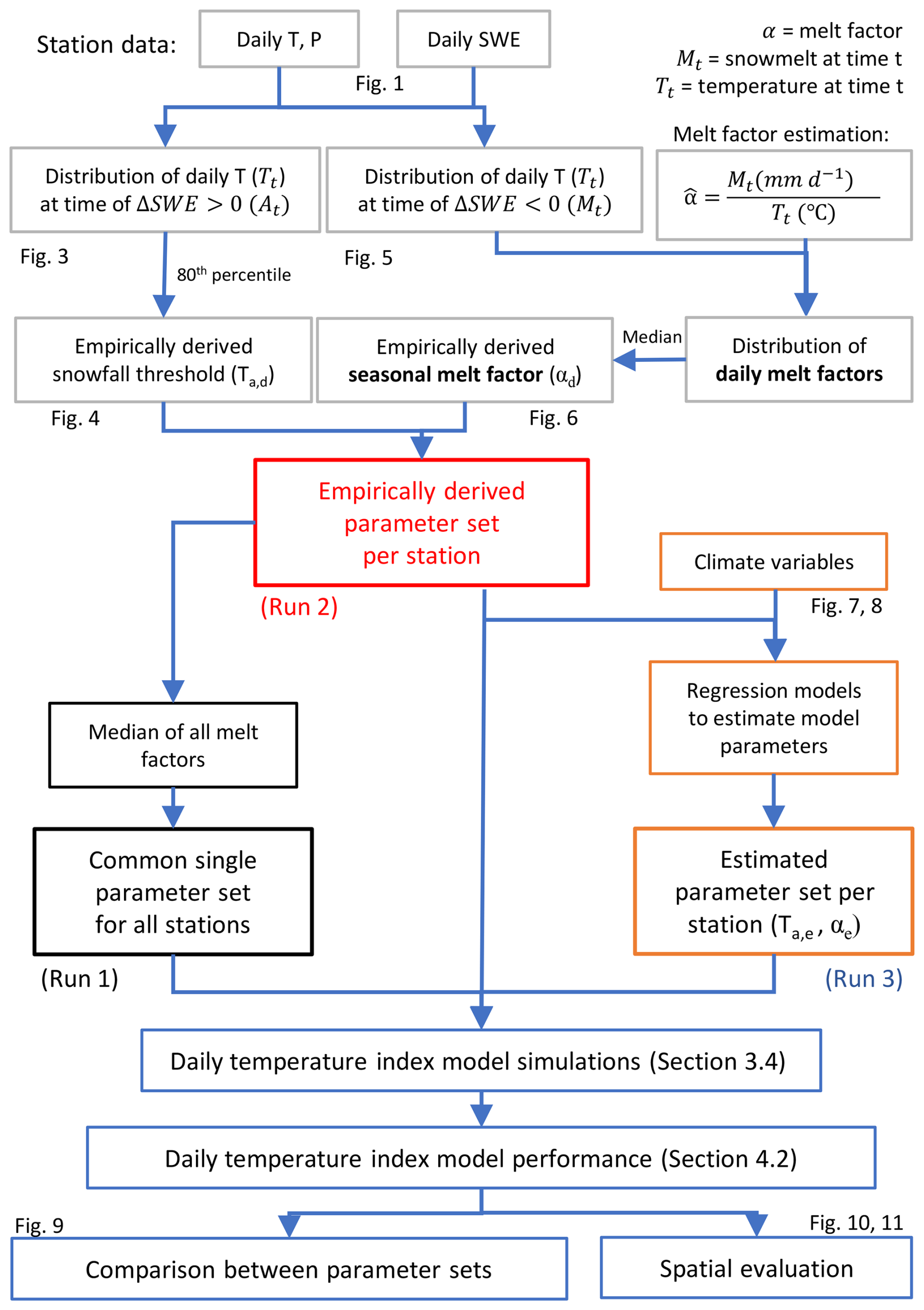
Figure 2 Flow diagram describing the temperature-index model simulations and the empirically derived and estimated parameter sets.

We evaluate the performance of the temperature-index model for important indicators of snow season dynamics, namely: accumulation season onset, melt season onset, end of snow season, peak SWE, number of snowmelt days, and snowmelt rate (Table 1). Timing errors are measured in days, with negative values indicating an early bias, and positive values indicating a late bias. Errors in peak SWE and snowmelt rates are expressed as relative percent error. We use these variables as indicators because they quantify important features relevant to our understanding of snow hydrology and because they provide a more comprehensive analysis of SWE time series performance than the typically used root-mean-square-error and the bias of the entire SWE time series. Note that for the empirically derived parameter set, performance is evaluated over the half of the available data at each station that is not used for deriving parameters. For the estimated parameter set, performance is evaluated over the $\mathrm{1}/\mathrm{3}$ of stations that are not used for parameter estimation.

3.5 Sensitivity analysis

We provide a sensitivity analysis of temperature-index model performance to the parameter choices and dataset splitting choices.

First, we test different values of the fixed temperature threshold for snow accumulation, and also a smooth temperature threshold for the rain-snow phase transition, as suggested in the literature (Dai, 2008; Jennings et al., 2025). We do this by varying the temperature threshold for snow accumulation from −0.5 to +1.5 °C in 0.5 °C steps for fixed thresholds. For smooth thresholds, we take a ±1 °C range around each fixed threshold, where precipitation is 100 % snow at the lowest end of the range and linearly decreases to 0 % snow at the highest end of the range. For each tested fixed and smooth threshold we repeat all model simulations and analyse model performance for total snowfall, peak SWE, and accumulation onset timing. Second, we analyse the sensitivity of the results to varying the snowmelt threshold from −0.5 to +1 °C in 0.5 °C steps. We then repeat all model simulations and analyse model performance for melt season onset timing and the end of snow season timing, as these are expected to vary with melt initiation thresholds. These sensitivity tests are applied to the first set of model runs (see Fig. 2).

Furthermore, we apply sensitivity tests for the second set (temporal split per station) and third set (spatial split for parameter fitting and validation) of simulations. For the temporal split of stations, we test whether splitting the station time series in the middle or randomly selecting half of the available years has an impact on the model performance. For the spatial split of stations, we check whether repeating the random split of stations ($\mathrm{2}/\mathrm{3}$ for model fitting and $\mathrm{1}/\mathrm{3}$ for model evaluation) has an impact on model performance.

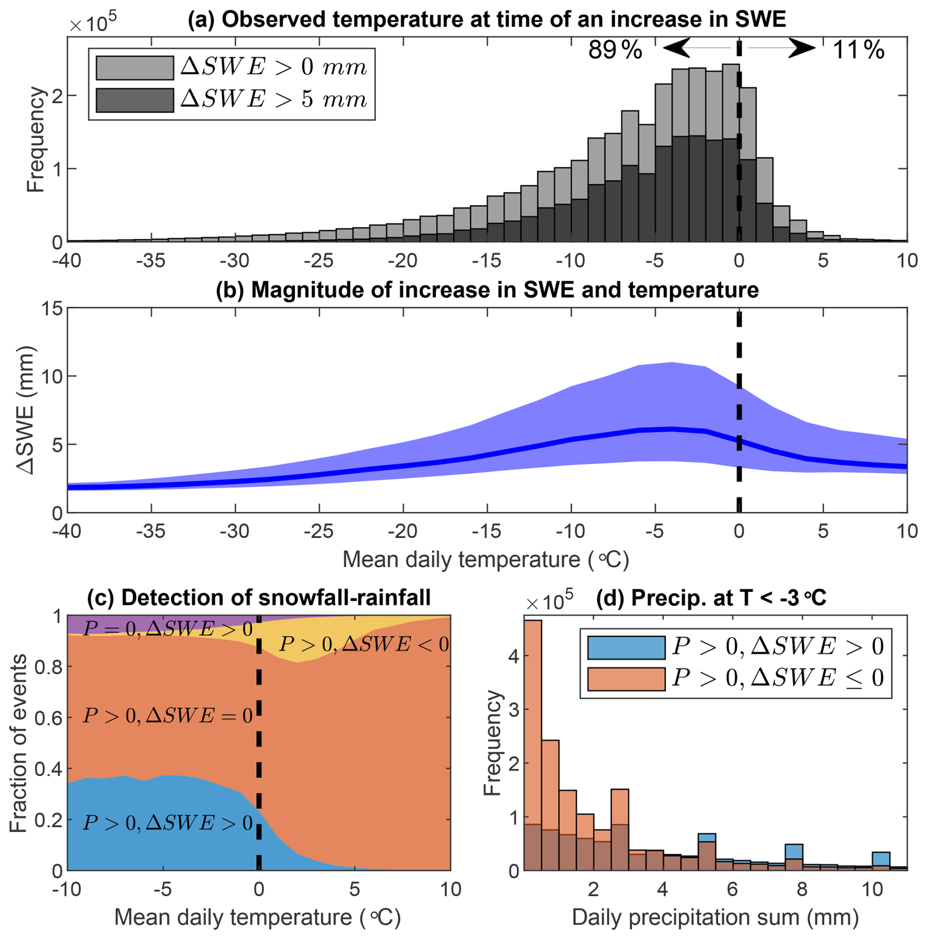
Figure 3 Analysis of observed temperatures at the time of snow accumulation. (a) Distribution of daily temperatures at the time of snow accumulation in the NH-SWE time series, for all snow accumulation time steps and for accumulations higher than 5 mm d⁻¹ only. (b) The magnitude of snow accumulation and daily temperatures. The solid line shows the median and the shaded area the interquartile range for each 2 °C bin between −40 and +10 °C. (c) Quality of snowfall-rainfall detection as a function of temperature, measured in terms of all possible situations that hint towards snowfall (i.e. precipitation P>0 or ΔSWE>0) or rainfall (P>0 and ΔSWE=0), including all contradictory events such as P=0 and ΔSWE>0. For each 1 °C bin between −10 and +10 °C, each case is coloured based on its fraction of occurrence. (d) Distribution of snowfall intensities for precipitation events at a temperature below −3 °C, detected (blue) and not detected (orange) by the NH-SWE time series. The darker parts of bars are the overlap of orange and blue.

4 Results

4.1 Derived and estimated temperature-index model parameters

4.1.1 Snow accumulation temperature threshold

We find that 89 % of all days with snow accumulation, i.e. with ΔSWE>0, occur with mean temperatures at or below freezing (0 °C), while only 11 % of snow accumulation days (empirically derived from the SWE time series) occur with mean temperatures above freezing (Fig. 3a). There are only 1 % of snow accumulation days at or above 5 °C. These do not necessarily suggest errors in the data since snow accumulation may occur on days with positive mean temperatures if those days have a strong daily temperature cycle (inducing subdaily freezing conditions) or if humidity is very low, i.e. low wet bulb temperature (Wang et al., 2019), or some combination of both.

If we filter out days with small snow accumulations (A_t<5 mm d⁻¹), the mean temperature conditions for snow accumulation contracts considerably, with only 5 % of accumulation days occurring at temperatures below −15 °C. This is supported by Fig. 3b, which shows that the magnitude of snow accumulation is limited at temperatures below −15 °C, physically consistent with a considerably diminished atmospheric moisture-carrying capacity at such low temperatures. The days with the largest snow accumulation occur between −7 and −2 °C, and accumulation amounts may still be large at $T_t>+\mathrm{1}$ °C, but quickly diminish for temperatures above this.

In Fig. 3c, we evaluate the quality of snowfall and rainfall days detection at a range of temperatures by comparing daily precipitation amounts observed at the climate stations to the daily changes in the SWE time series from the NH-SWE dataset. A summary of this detailed comparison is provided in Table 3.

Table 3 Summary and description of causes of (un)detected snowfall and rainfall days shown in Fig. 3c. Note that P_t refers to observed precipitation observed from the climate station time series, while the ΔSWE refers to changes in the SWE time series from the NH-SWE dataset. Colours in case column refer to Fig. 3c.

The results highlight a spectrum in the consistency between snow accumulation days detected based on snow depth observations (NH-SWE) and a simple temperature threshold together with precipitation observations. Below 0 °C, only roughly 35 % of the days with recorded precipitation (P_t>0) show a corresponding increase in SWE, which is a priori surprising: we would expect most precipitation to fall as snow below freezing air temperatures and accumulate on the ground. However, around 55 % of days with P_t>0 and T_t<0 °C do not show an increase in SWE. Figure 3d suggests that days with P_t>0, $T_t<-\mathrm{3}$ °C and ΔSWE≤0 are days with very small amounts of precipitation (P_t<3 mm d⁻¹). On those days, the resulting actual observed snow depth change is likely negligible; given that the SWE time series that we use here (Fontrodona-Bach et al., 2023b) are derived from snow depth observations (and not from actual SWE observations), SWE changes on these days cannot be detected.

In contrast, on days with P_t>0 and $T_t<-\mathrm{3}$ °C but ΔSWE>0 (i.e. days with SWE accumulation), the precipitation amounts are more uniformly distributed (Fig. 3d). Furthermore, below 0 °C, only about 10 % of the days show ΔSWE>0 and P_t=0, suggesting snowfall undercatch by the climate station, something widely reported in the literature (Adam and Lettenmaier, 2003; Kochendorfer et al., 2020; Pan et al., 2020).

Above 0 °C, most days with P_t>0 show ΔSWE=0, which is expected if precipitation is dominated by rainfall. It is also noteworthy that 20 % of days with 1 °C $<T_t<\mathrm{4}$ °C show P_t>0 and ΔSWE<0: this relatively large fraction represents days with rain-on-snow conditions, which could potentially enhance snowmelt rates and snowmelt days (Cohen et al., 2015).

A source of uncertainty from the analysis above is the potential for the co-occurrence of snow accumulation and snow melt within one day. Days with recorded precipitation and SWE loss (indicative of possible rain-on-snow or mixed processes) represent fewer than 10 % of events at 0 °C, and drop to less than 1 % at −5 °C (Fig. 3c). While the data in this study cannot resolve sub-daily variability, this limitation applies primarily to small magnitude accumulation and melt events occurring simultaneously. Larger snowmelt events during the melt season are confidently captured, as demonstrated by Fontrodona-Bach et al. (2023b), which shows minimal bias in total melt estimates.

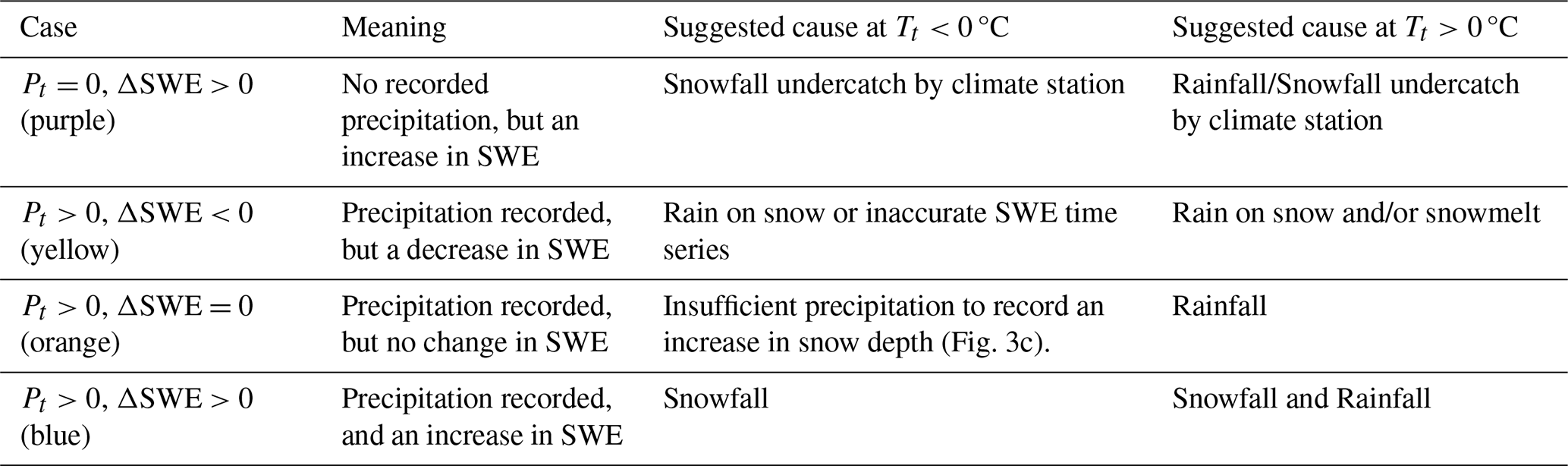
Figure 4 illustrates the linear regression model to estimate the snow accumulation temperature threshold based on climate variables (Eq. 5). The snow accumulation temperature threshold (empirically derived from SWE time series and corresponding temperature observations) varies across climates (Fig. 4). Very cold climates (high Δ_T and low $\stackrel{\mathrm{‾}}{T}$) have most snow accumulation days at temperatures below 0 °C, but more temperate climates have a larger fraction of snow accumulation days at 0 °C $<T_t<\mathrm{5}$ °C. While increasing the temperature threshold for snow accumulation might capture more of those above-freezing snow accumulation days, it also increases the false positive rate, i.e. recording actual liquid precipitation as snow accumulation.

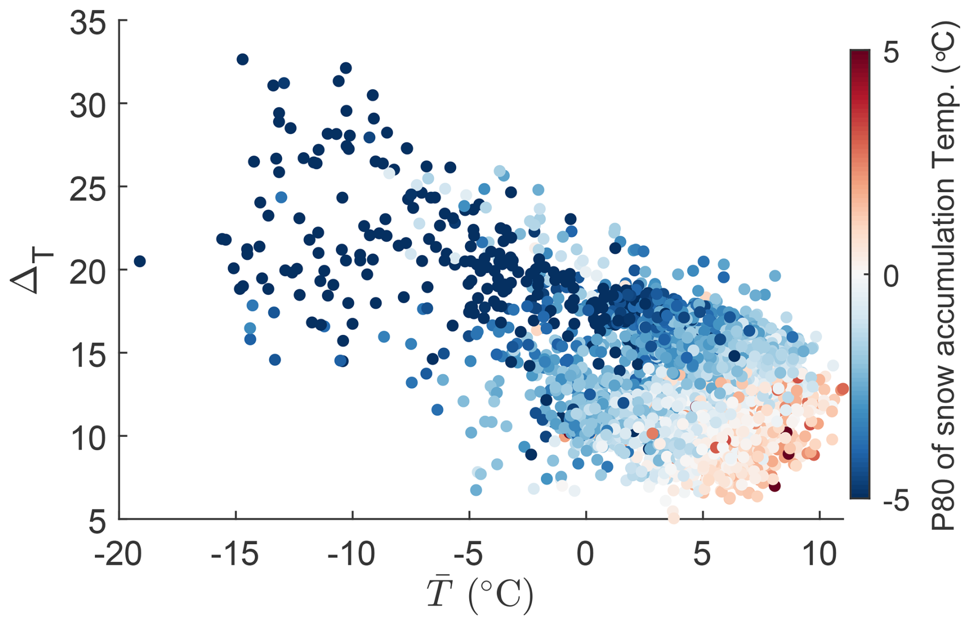
Figure 4 Snow accumulation temperature thresholds and climate variables (one point per station). Δ_T is the temperature amplitude of the climate and $\stackrel{\mathrm{‾}}{T}$ is the mean temperature of the climate (see Sect. 3.1). Colours show the snow accumulation threshold, defined as the 80th percentile of the observed daily temperatures on days when there is snow accumulation at each of the sites (see Sect. 3.3). Note these are only $\mathrm{2}/\mathrm{3}$ of the available stations, corresponding to the training set.

Figure 5 Analysis of observed temperatures for days with a decrease in SWE (ΔSWE<0). (a) Distribution of daily temperatures for days with a decrease in SWE in the NH-SWE dataset, either for all days with ΔSWE<0 mm or for days with $\mathrm{\Delta }\mathrm{SWE}<-\mathrm{5}$ mm. (b) Magnitude of decreases in SWE and daily temperatures. The solid line shows the median and the hatching shows the interquartile range, for each 1 °C bin between −15 and +15 °C. (c) Distribution of daily SWE changes (ΔSWE>0, ΔSWE<0, or ΔSWE=0) as a function of temperature. Lines based on histogram bins every 1 °C bin between −15 and +15 °C.

4.1.2 Snowmelt temperature threshold

Figure 5a shows that 76 % of daily decreases in SWE (ΔSWE<0) occur at daily temperatures above 0 °C and 24 % at temperatures below 0 °C. While snowmelt is only expected above freezing conditions, it is not unreasonable for snowmelt to occur at temperatures close to but below 0 °C, as the mean daily temperature may not capture subdaily positive temperature excursions or days near freezing conditions with high incidence of shortwave radiation. However, days with decreases in SWE during days with negative temperatures might also indicate other processes like sublimation, snow redistribution, or inaccuracies in either the temperature data or the SWE time series, but these appear very small in frequency and magnitude (Fig. 5a, b).

Above 0 °C, the magnitude of decreases in SWE scales linearly with temperature (Fig. 5b). Below 0 °C, decreases in SWE are low in magnitude and their frequency is small compared to the frequency of days with increase in SWE or no change in SWE (Fig. 5c). It is interesting to note that the distribution of the occurrence of increases in daily SWE and of decreases in daily SWE cross each other around 0 °C (blue and red lines in Fig. 5c), suggesting that below 0 °C it is more likely to have snow accumulation or no change in SWE, and above 0 °C it is more likely to have snowmelt days.

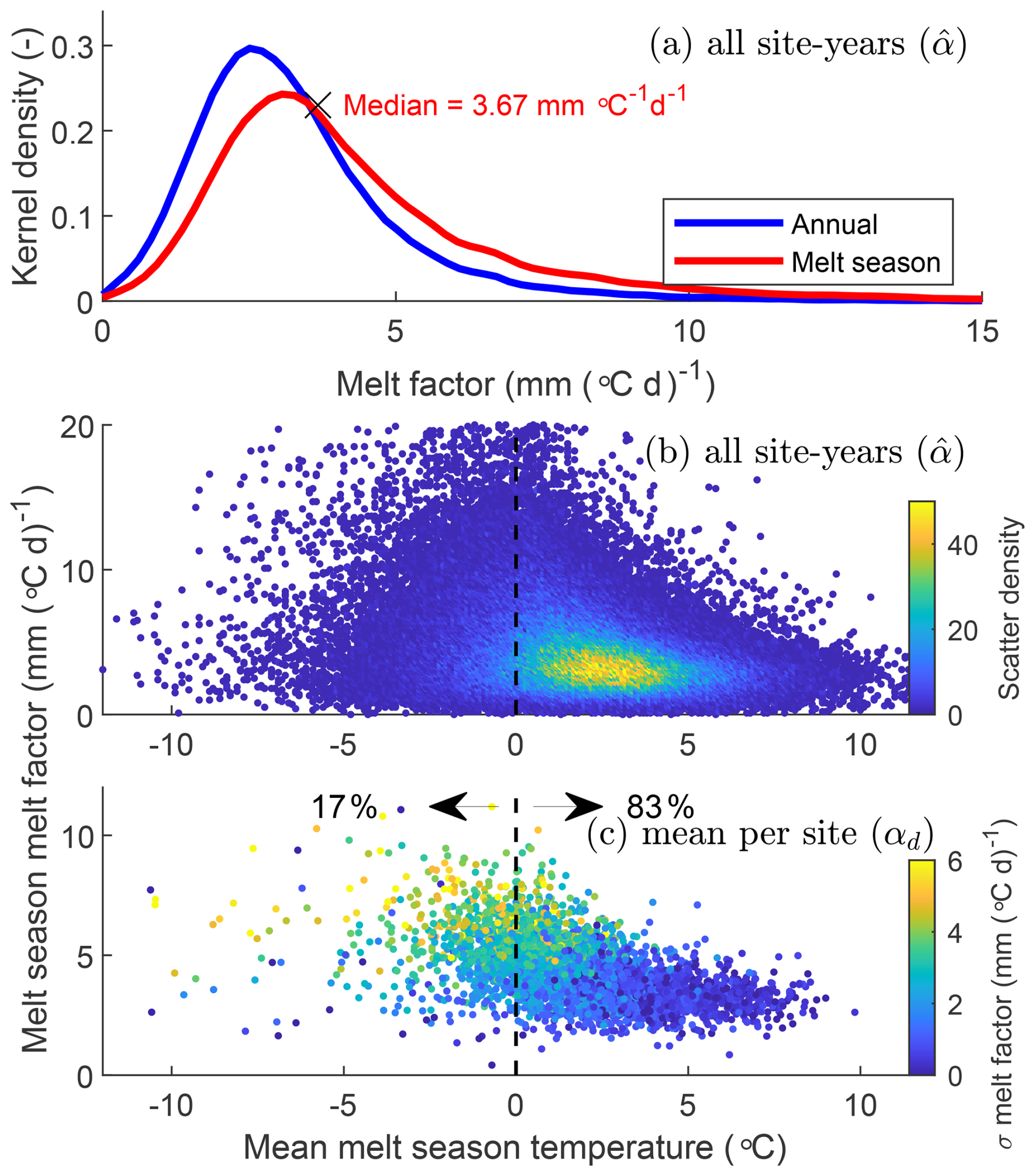
Figure 6 Empirically derived melt factors ($\widehat{\mathit{\alpha }}$ and α_d) and the link to melt season temperature and interannual variability. (a) Distribution of observed annual and seasonal melt factors. (b) Median melt season melt factor and mean melt season temperatures (all station-years). (c) Per station, mean melt factor, mean melt season temperature, and interannual variability (σ) of the melt factor.

4.1.3 Melt factor

Daily melt factors show a wide, but positively skewed, distribution of possible values and with a peak between 2 and 4 mm (°C d)⁻¹ (Fig. 6a). The median of all annual melt factors (2.93 mm (°C d)⁻¹) is slightly lower than for the melt season only (3.64 mm (°C d)⁻¹). This is likely because a decrease in SWE during the accumulation season typically occurs at lower net radiation inputs, and therefore melt factors (and melt rates) are lower. ns.

Melt factors vary with mean melt season temperatures (Fig. 6b, c). The range of possible melt factors is very large at mean melt season temperatures close to 0 °C, and most melt seasons have mean temperatures between 0 and 5 °C (Fig. 6b). The melt factor range converges to 3 to 5 mm (°C d)⁻¹ with increasing melt season temperatures (Fig. 6b). Only 17 % of stations have mean melt season temperatures below freezing (Fig. 6c). These stations with cold melt seasons show higher melt factors and a high interannual variability, limiting the predictive capacity of temperature-index models for these conditions. In contrast, 83 % of stations have positive mean melt season temperatures and lower melt factors, converging to 3 and 5 mm (°C d)⁻¹ and with far lower interannual variability.

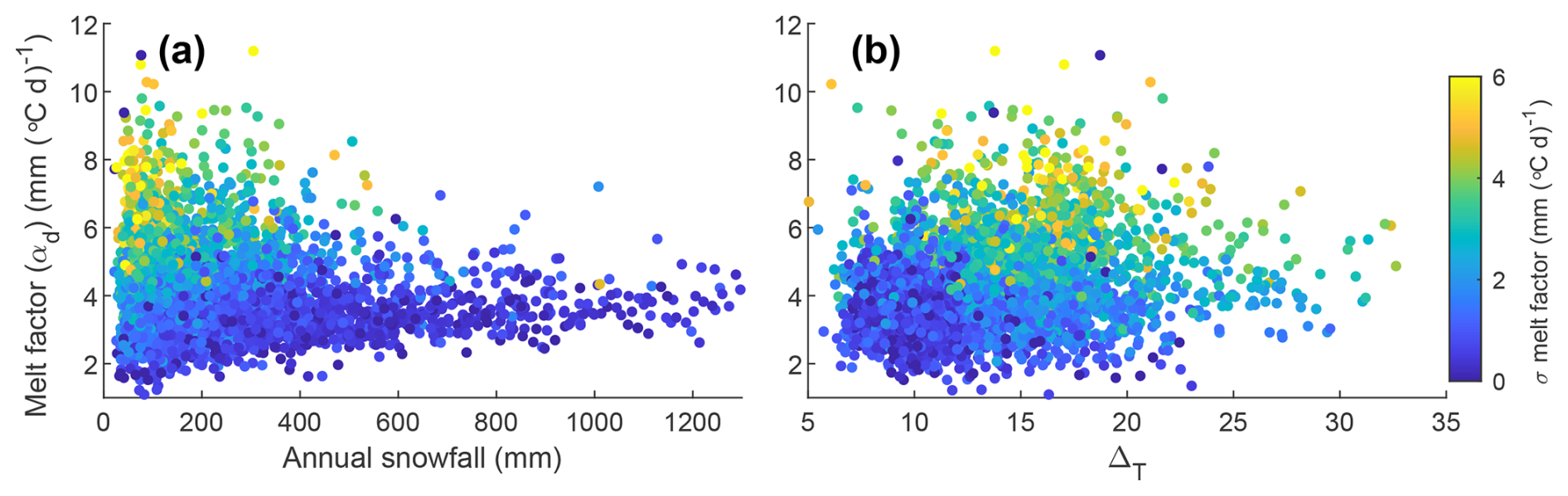
Figure 7 Climatic variability of the empirically derived (α_d) mean melt season melt factor. (a) Melt season melt factor and mean annual snowfall for each station; (b) Melt season melt factor and yearly amplitude of the temperature cycle. Both (a) and (b) are coloured by the interannual variability (σ) of the melt season melt factor.

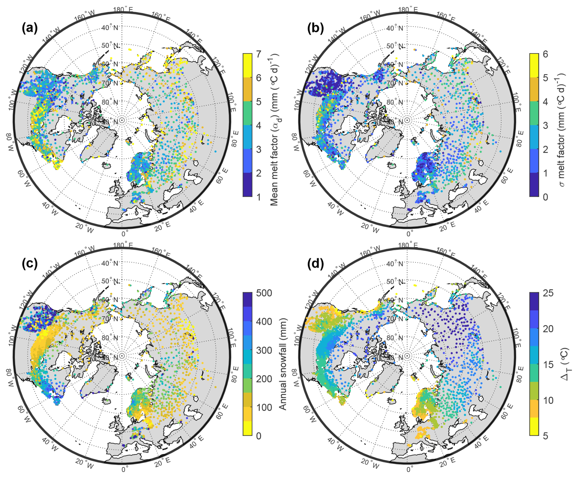
Figure 8 Spatial distribution of: (a) the melt factor (α_d), (b) its interannual variability (σ), (c) annual snowfall, and (d) the amplitude of temperature Δ_T.

We explore the variability across stations and across years in the mean melt season melt factor alongside climate variables in Fig. 7. The range of possible melt factors is very wide, from 1 to 12 mm (°C d)⁻¹, for stations with annual snowfall below 300 mm but converges towards 3–5 mm (°C d)⁻¹ for stations with annual snowfall above 300 mm (Fig. 7a). This convergence is also observed when comparing the melt factor and elevation (Fig. S2). Figure 7b shows that the mean melt factor and its interannual variability increase weakly with Δ_T; this is mostly driven by colder, more continental climates, with low precipitation, shallow snow, and late melt onset having higher melt factor values.

Spatially, the convergence of melt factor values to 3–5 mm (°C d)⁻¹ and low interannual variability (Fig. 8a, b) clearly occurs in areas with higher annual snowfall (Fig. 8c), and the more maritime (low Δ_T) and temperate (high $\stackrel{\mathrm{‾}}{T}$) climates (Fig. 8d), namely the mountain areas of Western North America, the European Alps, the Pyrenees and Scandinavia. Outside these deeper snowpack areas, for colder climates with shallower snowpacks, such as continental North America and Eurasia, it is clear that melt factors are higher and spatially more variable.

Despite the variability of the melt factor with melt season temperatures (Fig. 6), climate (Fig. 7) and its geographical distribution (Fig. 8), our melt factor estimation model based on station geography and climate did not yield a good predictive skill (R²=0.16). Our melt factor estimation model (Eq. 7) shows that melt factors decrease with elevation, which is opposite to what Hock (2003) suggested. This probably results from the convergence towards lower melt factor values (3–5 mm (°C d)⁻¹) that our analysis shows for deeper snowpacks, which are common at higher elevations. Similarly, the melt factor also decreases with increasing latitude. The estimated melt factor increases with lower mean temperatures, which could be expected because the shortwave radiation component for melt becomes more important. The high interannual variability of the melt factor on some climates could partly explain the low predictive skill of the linear regression model of Eq. (7).

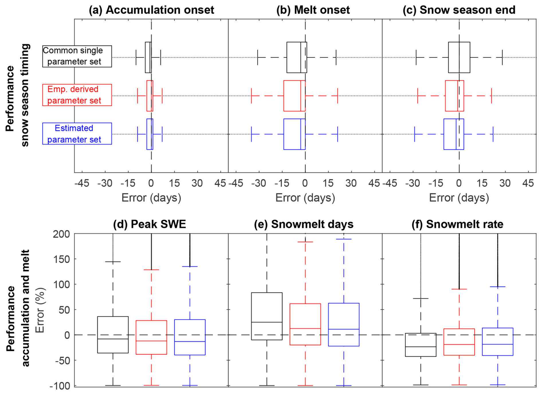
Figure 9 Temperature-index model performance. The three sets of model simulations (Table 2) are shown in each boxplot, namely the common parameter set for all stations, the empirically derived parameter set for each station, and the estimated parameter set for each station. Boxes are built with all station-years in the analysis. (a, b, c) Performance of the three snow variables related to timing of the snow season. (d, e, f) Performance of the three snow variables related to magnitude of accumulation and melt in the snow season. Note that outliers are shown as points outside the box whiskers.

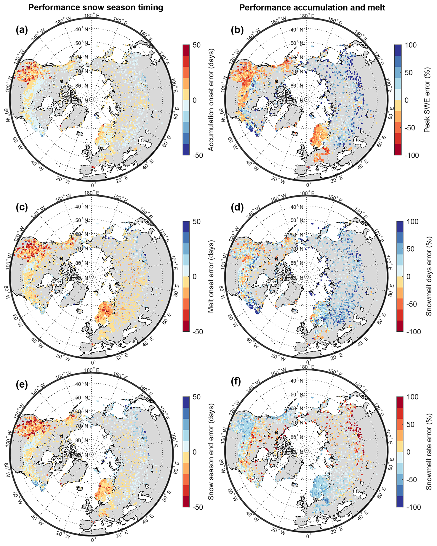
Figure 10 Spatial distribution of temperature-index model performance. (a, c, e) for snow season timing variables, and (b, d, f) for snow season accumulation and melt magnitude variables. The median error for each station is shown for the simulation using the estimated parameter set.

4.2 Temperature-index model performance

4.2.1 Overall performance

The performance of the temperature-index model is generally very good (Fig. 9), especially considering the simplicity of the model and that the parameters were empirically derived from the data or estimated from climate variables but not calibrated to improve performance. Importantly, all snow season timing variables show median errors close to zero days, and interquartile ranges do not exceed a 15 d error (Fig. 9a, b, c). Especially excellent is the performance of the timing of the accumulation season onset, where even the whiskers do not exceed a 15 d error for any of the three sets of model simulations. Regarding the melt season onset, all three simulations show a median timing that is 4 d too early. However, it must be noted that the validation data (the NH-SWE dataset) showed an average model delay of 2 d in the onset of the melt season (Fontrodona-Bach et al., 2023b), which suggests that the median error in Fig. 9b may actually be closer to zero. Given that the melt season onset depends mostly on the snowmelt threshold temperature, which is the same for all simulations, it is unsurprising that all three simulations show an almost equal performance for this variable. For the end of the snow season timing, the differences between the simulations are more visible but still relatively minor. This minor difference is due to the high dependence on the melt factor, which is estimated differently in all three sets of simulations. Simulations with the common parameter set have a better median error, likely because the melt factor used is the median of all stations. Simulations with the empirically derived parameter set have a narrower interquartile range, as values are empirically derived from observations at each station individually. Simulations with the estimated parameter set have a slightly worse, though comparable, performance.

Regarding snow season accumulation and melt magnitude variables, the temperature-index model shows good median errors across variables and parameter sets, but also has large interquartile ranges and whiskers, and many outliers (Fig. 9d, e, f). Interquartile ranges for peak SWE are within 45 % error, and the median values display a negative bias at around −10 % error. No significant differences arise between parameters sets for peak SWE. The whiskers and outliers, however, extend to very large errors, from −100 % to +200 %. Relative errors in peak SWE are largest at stations with very shallow snowpacks (<100 mm, Fig. S3). For such sites, small absolute deviations translate to large relative errors (e.g. 100 mm modelled vs 10 mm observed $=+\mathrm{1000}\mathit{\%}$). However, for stations with deeper snowpacks, errors are consistently lower. Median underestimation for snowpacks with peak SWE higher than 100 mm is −25 %. This shows that, while outliers are prominent, they are concentrated in a specific subset of sites and not indicative of general performance.

For snowmelt days, simulations using the empirically derived and estimated parameter sets have a similar median of 10 % and 8 % error, while simulations using the common parameter set performs slightly worse with a median 20 % error overestimation of the number of snowmelt days. For snowmelt rate, the common parameter set also performs slightly worse (−25 % error) than the empirically derived and estimated ones (−22 % error). Simulations across all parameter sets underestimate the snowmelt rate but have the narrowest interquartile range of the three snow accumulation and melt magnitude variables.

We also tested the effect of different fixed and smoothed snowfall-rainfall partitions thresholds on model performance. At the daily scale, no single fixed threshold for snow accumulation classifies rain-snow optimally: low thresholds tend to misclassify snow days as rain, while higher thresholds misclassify rain as snow (as shown in Fig. S4, which zooms in on Fig. 3c). Interestingly, a lower threshold fixed threshold than the one we used (e.g., 0 °C) improves estimates of total snowfall and accumulation onset by reducing false accumulation on ephemeral snow days outside the core season (Fig. S5 top panel). Conversely, a higher threshold (e.g., 1.5 °C) improves peak SWE by reclassifying marginal rain events as snow (Fig. S5 middle panel). Smooth thresholds, where snowfall probability transitions linearly between two temperatures, offer only marginal improvements for total snowfall but do not improve peak SWE or snow accumulation onset (Fig. S5). At daily resolution, uncertainty in the timing of precipitation events makes the application of these smoother temperature thresholds less straightforward.

Given the overall similar performance between the three sets of simulations, only peformance results using the estimated parameter set are shown in Fig. 10, for the testing set of stations only. This demonstrates clear spatial differences, where snow season timing variables (Fig. 10a, c, e), show the mountain areas of Western North America as well as Scandinavia have poorer performance, with late accumulation season onset, early melt season onset, and early end of the snow season. Performance is much better over the rest of the Northern Hemisphere and for all three timing variables.

Performances of snow accumulation and melt magnitudes show marked differences between Northern Hemisphere regions, especially for peak SWE (Fig. 10b). Many stations underestimate peak SWE in North America and over Europe, while overestimations are observed in Canada and Eurasia. However, in these stations the underestimation of peak SWE does not inherently lead to fewer snowmelt days, since the snowmelt rate is also underestimated. In contrast, data from stations across the rest of the Northern Hemisphere mostly overestimate the number of melt days (Fig. 10d), suggesting that the melt temperature threshold or melt factor might not be accurate for these stations. Figure S6 suggests melt onset initiation actually peaks at air temperatures between 1 and 3 °C, which highlights a small but significant disconnect between air and snow temperatures that may also explain the negative bias in the timing of melt onset using the zero degrees threshold assumption. In fact, a slightly higher threshold (0.5 °C) does improve melt onset estimation (Fig. S7), but this same adjustment degrades performance in predicting snow season end dates, which are more sensitive to daily temperatures near 0 °C once melt has already begun.

Finally, melt rates show both the smallest and most spatially consistent relative errors of all three variables (Fig. 10f), generally not exceeding 10 %. The melt rate errors also have some spatial structure, with underestimation generally occurring in regions with deeper snowpacks, such as Western North America, Scandinavia, and the European Alps, and overestimation in regions with shallower snowpacks, such as Northern Canada and some stations in East Asia.

4.2.2 Sensitivity analysis

The sensitivity tests for fixed and smooth snow accumulation thresholds and melt thresholds show that choosing different thresholds does not consistently improve model performance across snow variables (Figs. S5 and S7) when applied consistently across all stations. The median performance and the distribution of performance shifts to a better performance for some variables and to worse performance for other variables. It therefore seems challenging to consistently improve model performance of a daily temperature-index snow model when applying uniform parameters across diverse snow climates.

The overall model performance of the second and third set of model simulations did not materially change regardless of how the temporal split of stations was done and also not by repeating the random split of spatial stations. For the fixed melt factor in the first set of model simulations (see Table 2), a 1000-replicate random half-sample test of all stations yields medians 3.61–3.66 mm (°C d)⁻¹, indicating the common value is robust and that the results are negligibly affected by which half is used. The parameter estimation model fits (Eqs. 5 and 7) changed marginally when repeating the station split 100 times (snowfall threshold R²: range 0.66 to 0.69; melt factor R²: range 0.17 to 0.12).

4.2.3 Climate clustering

Because of the marked and consistent spatial differences in performance, we created three snow climate clusters using k-means clustering (MacQueen, 1967) and five climate or site characteristics defining each snow climate cluster: elevation of the station, mean peak SWE, mean snow cover duration, mean temperature, and temperature amplitude. The best silhouette score (Rousseeuw, 1987) (0.70) was given by three snow climate clusters.

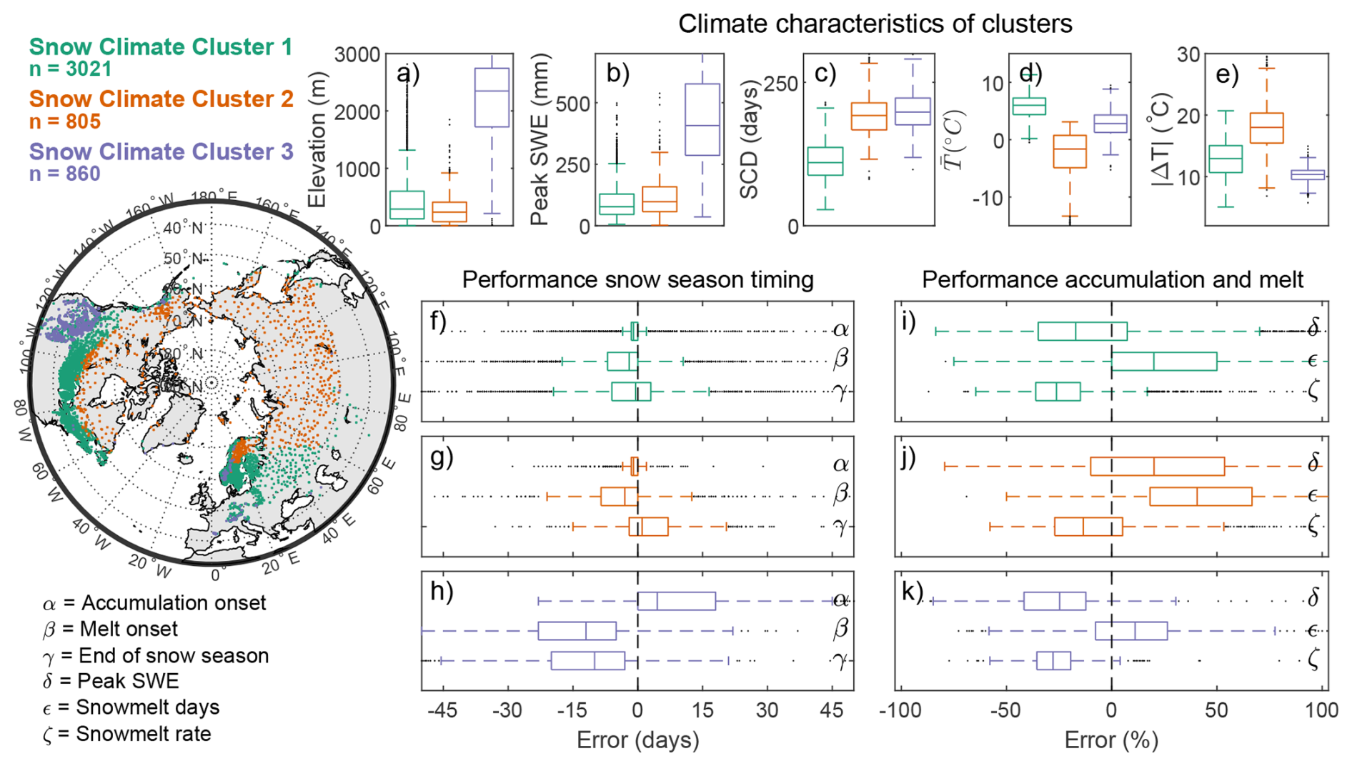
Figure 11 Snow climate clustering and model performance. The map shows the spatial distribution of the three snow climate clusters. Panels (a)–(e) show site and climate characteristics of the stations in each cluster. Panels (f), (g), (h) show the model performance of Cluster 1, 2 and 3 (respectively) for the three snow season timing variables (accumulation onset, melt onset, and the end of snow season). Panels (i), (j), (k) show the model performance of Cluster 1, 2 and 3 (respectively) for the three snow accumulation and melt variables (peak SWE, snowmelt days, snowmelt rate).

Cluster 1 is the most abundant, with 3021 stations. These are low to mid elevation stations with relatively shallow snowpacks (Table S1 in the Supplement, Fig. 11a, b), with the lowest snow cover durations and the warmest of the climates considered (Table S1, Fig. 11c, d, e). These are located in temperate and maritime areas in Europe and North America. This cluster has the best performing scores for snow season timing variables and for peak SWE despite a dominance of peak SWE underestimation (Table S1, Fig. 11f, i).

Cluster 2 has 805 stations located over shallow but long lasting snowpacks in the coldest and most continental climates considered, such as North and East Asia, and the most northern parts of Scandinavia and North America (Table S1, Fig. 11a–e). This cluster has very good performance for snow season timing variables and is characterised by a consistent overestimation of peak SWE (Table S1, Fig. 11g, j).

Cluster 3 has 860 stations and is characterised by deep snowpacks and mostly higher elevations, long snow cover durations, and cold climates (low mean temperature and low temperature amplitude, located over western North America, the European Alps, and the Scandinavian mountains (Table S1, Fig. 11a–e). These are characterised by a too late onset of the accumulation season as well as too early melt onset and too early snow season end (Table S1, Fig. 11h). This cluster has the lowest median performance in peak SWE, but the most consistent (lowest range of the interquartile range) (Table S1, Fig. 11k).

All three clusters have in common a consistent overestimation of melt days and an underestimation of the melt rate. Outliers in Fig. 11 are a minority and range from 2.4 % to 21.7 %, therefore never exceeding 10.9 % of points on each side of the zero error line.

Overall, the simple temperature-index model performs remarkably well for most input data and stations, but there can also be large variance, and it occasionally performs poorly. Examples of this range of excellent, good, acceptable and poor performances are provided as time series in Fig. 12. In the next section, we discuss potential reasons for the range of performances.

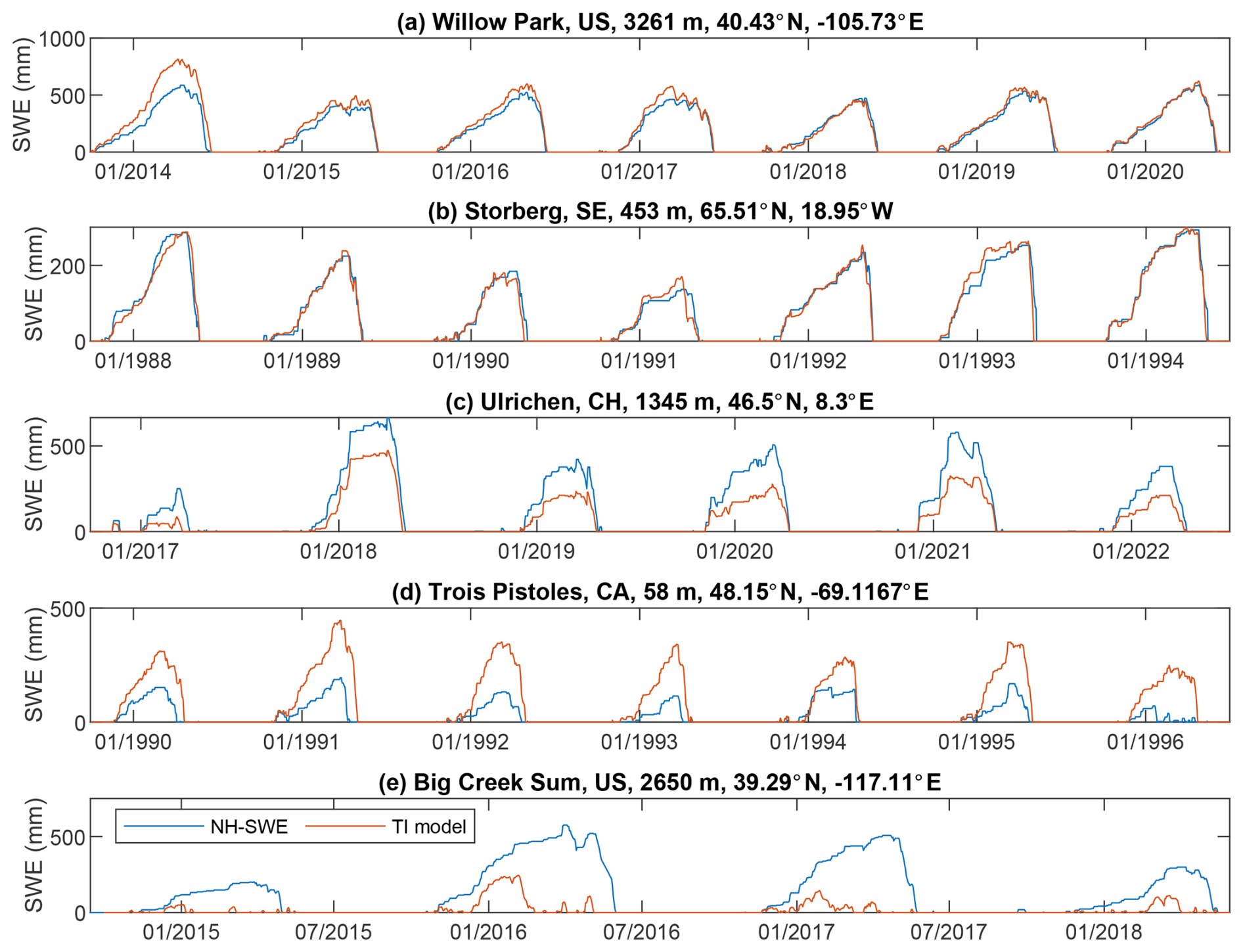
Figure 12 Example SWE time series comparison vs temperature-index model simulations with the estimated parameter set. Good (a, b), medium (c) and poor (d, e) performances across different regions. Title of each subpanel shows the station name, country code, elevation in metres, latitude and longitude.

5 Discussion

5.1 Snow accumulation temperature thresholds

Our analysis highlights the range of temperatures at which snow accumulation events occur and shows that most accumulation days occur at daily average temperatures below freezing. This is broadly in accordance with previous studies (Rohrer and Braun, 1994; Magnusson et al., 2019), but we now provide this evidence at much larger spatial and temporal extents. This highlights the potential of a simple snowfall air temperature threshold to capture most snowfall days successfully, especially for cold, continental climates with shallow snowpacks (e.g., North/East Asia, continental Canada). However, our results also highlight that some relatively large snow accumulation days at daily average temperatures close to, but just above freezing temperatures, are difficult to capture. The risk of missing snow accumulation days can be higher in warmer maritime climates with deeper snowpacks (e.g. western North American mountains, the European Alps, or Scandinavia) at near freezing temperatures. While a 0 °C threshold captures most events, regional adjustments or wet-bulb thresholds are preferable in climates with frequent near-freezing precipitation. Therefore, where snow accumulation days above freezing temperatures are critical to capture, we emphasise the importance of using a different precipitation phase method, such as the use of wet bulb temperature (Jennings and Molotch, 2019), if available. Alternatively, snow accumulation temperature thresholds may be adjusted regionally, as our analysis in Figs. 3 and 4 shows that warmer climates generally have higher snow accumulation temperature thresholds.

While a temperature-based precipitation phase threshold may miss snowfall days above freezing, they are well captured by snow observations. Conversely, snowfall days are well captured at temperatures well below the snowfall threshold. It is important to note that time series of snowpack observations may also fail to register precipitation days if they are small (<3 mm), which is typical of cold climates, such as Northe/East Asia and continental Canada. Additionally, our analysis suggests that rain-on-snow days during the melt season are more frequent and widespread than previously recognised. Undercatch of solid precipitation in rain gauges is also observed (ca. 10 % of fraction of precipitation days below freezing). It is important to note that the daily time scale nature of our approach limits the possibility to capture sub-daily variability, and the co-occurrence of snow accumulation and snowmelt within one day. However, our analyses show that these are small in frequency and magnitude and do not materially impact our results and conclusions. In the context of long-term performance of a temperature-index model at the daily scale, it is important to emphasise that our data clearly demonstrates that no snowfall threshold, fixed or smooth, consistently improves all metrics or reduces interquartile uncertainty ranges. This suggests that, although the temperature-threshold approach for snow accumulation is satisfactory on average, further performance improvements are challenging to achieve, highlighting the inherent limitations of the temperature-index approach.

5.2 Melt temperature thresholds

We have tested the validity of a simple temperature threshold of 0 °C to capture snowmelt using an observation dataset at the largest spatial and temporal scale to date. The data clearly indicate that snowmelt occurs almost exclusively at daily average air temperatures above 0 °C, as evidenced by the sharp decrease in the frequency of days with no change in SWE as temperatures rise above this value and the linear increase of snowmelt magnitude with temperature (Fig. 5). Temperature-index snow models often choose a value of 1 °C (Avanzi et al., 2022), 0 °C (Senese et al., 2014) or even −1 °C (Elias Chereque et al., 2024) as the threshold for snowmelt initiation. Overall, our results highlight snow accumulation and snowmelt days reach an equal frequency of occurrence at air temperatures around 0 °C, suggesting this is an appropriate air temperature threshold for most data in a large-scale study. However, we also find that to accurately predict the onset of the melt season, a slightly higher air temperature threshold may be required (Figs. 9 and S6). This is likely because zero degree snowpacks still need to overcome the latent heat of fusion to initiate snowmelt (Molotch et al., 2009; Jennings et al., 2018a), and thus air temperatures may be slightly higher than zero during actual melt initiation. However, this degrades the predictive accuracy of the end of the snow season (Fig. S7), which is more sensitive to daily temperatures near 0 °C once melt has already begun. It must also be noted that the NH-SWE time series used for validation exhibited a slight delay on average in melt season onset (Fontrodona-Bach et al., 2023b), thus it is possible to speculate this could reduce the overall uncertainty in melt onset for the temperature-index model results presented here.

As with snow accumulation thresholds, these results highlight trade-offs, whereby adjusting thresholds improves performance for some variables at the cost of others. Interquartile ranges remain broadly similar across threshold choices, suggesting that model performance is relatively insensitive to the precise value of the threshold within the ranges we tested.

5.3 Melt factors

We have shown that melt factors vary substantially across spatial and temporal scales. Seasonal scale melt factors across the Northern Hemisphere ranged from 1 to 12 mm (°C d)⁻¹, in accordance with ranges estimated in the literature from individual sites at smaller spatial scales (Braithwaite, 1995; Kane et al., 1997; Lefebre et al., 2002; Hock, 2003; Braithwaite, 2008; Shea et al., 2009; Asaoka and Kominami, 2013). While these literature sources find most common melt factors to range between 2 and 6 mm (°C d)⁻¹, our results further refine this range and show there is a clear dominance of melt factors between 3 and 5 mm (°C d)⁻¹, particularly in regions with deeper snowpacks and more temperate climates. This key finding suggests that melt factors tend to stabilise within these specific climatic conditions, which also tend to have warmer melt seasons. Furthermore, the low interannual variability of these melt factor values suggests that climatic conditions with deep snowpacks and temperate climates are conditions that are well suited for temperature-index modelling. For these deeper snowpacks, the dominant snowmelt energy sources are probably similar year to year, making the melt factors less variable and easier to predict. In contrast, it may be harder to robustly estimate melt factors for colder, continental climates with shallower snowpacks, as they typically exhibit higher melt factors with higher interannual variability. For these shallower snowpacks, it is likely that the partition of snowmelt energy sources varies from year to year, making the melt factors more variable. In addition, our results suggest other loss mechanisms, such as sublimation or snow redistribution by wind, are more common in these colder, shallower snowpack climates. As a result, temperature-index melt modelling will likely provide a poorer representation of SWE dynamics in these conditions, as other accumulation or loss mechanisms that are typically more important during the accumulation season may not be captured by the temperature-index approach.

5.4 Long-term, hemispheric scale temperature index model performance

The median performance of the temperature-index model across various indicator variables for a wide range of climate conditions across the Northern Hemisphere is surprisingly good given the model's simplicity and that parameters were only estimated from data, and not calibrated to improve model performance. Evaluation of snow season timing variables across the Northern Hemisphere showed a median error of 0 d for the accumulation onset, 4 d early for the melt onset, and 1–2 d early for the end of the snow season. This shows the long-term time series dynamics are, on average, well captured by the temperature-index approach. Nevertheless, our climate clustering analysis suggests that accurate snow cover timing dynamics are best captured for shallow (peak SWE <300 mm) and mid to low elevation snowpacks (<1500 m), while deeper (peak SWE >300 mm) or higher elevation (>1500,m) snowpacks show a worse performance. This is probably linked to an increased complexity of temperature and precipitation processes and their measurements over alpine areas (Collados-Lara et al., 2018).

Regarding snow accumulation and melt magnitude variables, a median relative error of −10 % was found for peak SWE, a median relative error of +10 % for the number of snowmelt days, and a median relative error of −22 % for the snowmelt rate. These results highlight the excellent performance that the temperature-index models can achieve if the input data is of high quality and if most snowfall days occur at temperatures below 0 °C. However, the temperature-index model underestimates peak SWE especially for deeper snow climates (e.g. western North American mountains, the European Alps, and the Scandinavian mountains), where a negative bias is observed for up to 75 % of stations (Cluster 3). This is consistent with our analysis and highlights a possible combination of undercatch of solid precipitation, the inability of the temperature threshold to capture snow accumulation days above freezing, the potential underestimation of the snowmelt initiation temperature threshold, climate station measurement errors, or residual uncertainties with the validation dataset.

It is challenging to point out the exact cause of errors in peak SWE as it can be a combination of factors relating to accurately capturing accumulation and melt during the accumulation season. At the stations in Cluster 2 (shallow, long lasting snowpacks in the coldest climates), the peak SWE overestimation is linked to too much precipitation as snow accumulating on the ground compared to the observations (Fig. S8c). In these cold and more continental climates it is likely that drier low density snow is subject to redistribution processes not captured by the temperature-index model, leading to an overestimation of peak SWE. At the stations in Cluster 3 (deep, mostly high alpine snowpacks) the peak SWE overestimation is linked to not enough precipitation as snow accumulating on the ground during the accumulation season (Fig. S8e), which could be linked to increased measurement complexity in alpine areas, such as undercatch (Cho et al., 2022) but also missing snow accumulation events at mean daily temperatures just above freezing not captured by the temperature-index model, as discussed in Sect. 5.1.

During the accumulation season, the temperature-index model shows more melt than observed for all clusters (Fig. S8b, d, f), but this could also be because of the already discussed limitation that the NH-SWE dataset may not capture small melt events during the accumulation season. Our analysis therefore suggests that inaccurately capturing precipitation is the main culprit for errors in peak SWE. Furthermore, feedbacks to other metrics arising from errors in peak SWE may occur. For instance, a temperature-index model underestimation of peak SWE may, in turn, result in an underestimation of the number of melt days, but an underestimation of the snowmelt threshold temperature may overestimate the number of days with melting conditions and compensate for the underestimation of melt days.

Contextualising these results is not straightforward because a direct comparison to other models is not possible at this scale, due to the lack of input data and information on appropriate parameter ranges. However, we can offer a useful benchmark by comparing reported performances from recent model evaluations. Menard et al. (2021) report peak SWE biases from −50 % to +35 % across ESM-SnowMIP models (Krinner et al., 2018). Cho et al. (2022) found that land surface models underestimated peak SWE by 268 mm on average at SNOTEL sites. In comparison, our TI-based approach underestimates peak SWE at SNOTEL sites by 114 mm on average, and the timing of peak SWE is 23 d early vs. 36 d early reported by Cho et al. (2022). While such comparisons are not one-to-one, they demonstrate that TI models, when interpreted cautiously, can yield useful constraints. Even for the worst performing climate clusters, most stations showed a reasonable performance, showing that simple approaches can be applied across climates, with known limitations described in this paper.

The temperature-index model performance analysis suggests that the estimated melt factors are relatively robust. Snowmelt rates, which should be the model performance indicator most sensitive to melt factor accuracy, have smaller relative errors than peak SWE and the number of melt days. However, it may also suggest that despite the challenges in estimating melt factors for colder and shallower snowpacks (as outlined above), melt rate model performance is not overly sensitive to melt factor accuracy, as melt rate estimates are consistently robust even under conditions where the melt factor experiences high interannual variability. In fact, the mean melt rate is more strongly linked to the mean melt season temperature than the mean melt factor (Fig. S9), suggesting that accurate temperature data and a reasonable melt factor value can yield robust model performance across the Northern Hemisphere. In any case, an important implication is that melt rates can be more confidently estimated using temperature-index models than some of the other key snow metrics (such as peak SWE and melt onset) evaluated here. However, it is important to note that any trend introduced by climate change impacts may complicate the robust estimation of melt factors (Raleigh and Clark, 2014; Musselman et al., 2017).

A striking result of our study is the small difference between the three parameter sets used for model simulations, and in particular that the simulations with the single common parameter set perform comparably, and better in some metrics, than the simulations with the empirically derived and estimated parameter sets (as seen in Fig. 9). There are a variety of reasons leading to small differences in model performance between the three parameters sets. First, the melt temperature threshold is the same for all sets of simulations, which limits the possible differences in results. Second, the snow accumulation temperature threshold varies per station but only minimally, as we set a minimum value of 0 °C. For the empirically derived and estimated parameter sets, 79 % and 86 % of stations have a threshold value of 0 °C, respectively. For the rest of the stations, values are mostly below 2 °C (Fig. S10). The final factor contributing to variability in model performance across parameter sets is the melt factor. The empirically derived and estimated melt factors are weakly correlated (R²=0.13, Fig. S11), showing that differences are big between parameter sets. However, the model performance metrics most sensitive to the melt factor (the melt rate and the timing of the end of the snow season) exhibit strong correlations between parameter sets (R²=0.70 and R²=0.62, respectively, Fig. S12). This indicates that model performance is not very sensitive to model parameters, at least when evaluated over long-term time series, and suggests that for long-term studies using temperature-index modelling, it is not necessary to use complex parameter estimation methods, as the use of commonly applied values in the literature will lead to similar model performances.

6 Conclusions

Using a new Northern Hemisphere SWE dataset, our paper investigates the performance, assumptions, limitations, variability and parameter sensitivities of the temperature-index (TI) modelling approach across a wide range of Northern Hemisphere snow climates. While the goal of this study was not to develop or optimize a new TI model, our analysis offers several novel contributions.

The findings highlight the significance of temperature thresholds in governing snow accumulation and snowmelt events and in their simulation using a simple TI model. Our results are in line with the widely accepted physically based threshold of 0 °C separating accumulation from melt processes. While a temperature-based precipitation phase threshold captures most snow accumulation events on a daily scale, the risk of missing substantial snow accumulation events, particularly in climates receiving precipitation near freezing temperatures, must be considered.

Our results clearly show that most decreases of SWE (i.e. melt events) occur at daily temperatures above freezing and that the melt rate scales linearly with temperature. Decreases of SWE below freezing in the NH-SWE dataset are likely not snowmelt events but sublimation or snow redistribution processes. The study highlights the equal frequency of snow accumulation and snowmelt events occurring at a temperature of 0 °C, making this a suitable threshold for large-scale studies. However, our results also suggest the potential need for a slightly higher temperature threshold to initiate the snowmelt season. Accounting for the 2 d delay in melt onset in the NH-SWE time series, the effective bias in our model estimates of melt onset may be closer to 0 d.

Our sensitivity analysis of temperature thresholds shows that, at the spatial and temporal scale considered in our study, adjusting the temperature thresholds does not consistently improve performance across all snow metrics of interest. In other words, the temperature-threshold approach yields overall good results with temperature thresholds (accumulation and melt) set to 0 °C, but a further model performance improvement would require a joint optimisation of both threshold parameters to individual station data or for different climates (which was not the objective of our work).

The investigation of melt factors offers insights into their variability across climatic conditions. Melt factors converge to 3–5 mm (°C d)⁻¹ and show a low interannual variability in regions with deeper snowpacks (peak SWE >300 mm) and temperate climates, making the estimation of melt factors very robust. However, our study highlights challenges in estimating melt factors for colder, continental climates with shallower snowpacks due to higher interannual variabilities. Still, the model performance was not worse in those regions because the mean snowmelt rate is more sensitive to the mean melt season temperature than to the melt factor.

The temperature-index model consistently captures snow season timing, although minor deviations in melt season initiation and end are noted. Our results highlight the model's challenges in estimating peak SWE and the number of melt days, particularly in alpine regions with deeper snow climates, where peak SWE is generally underestimated, attributed to factors including undercatch of solid precipitation, temperature thresholds, and potential data errors. In cold, continental regions with shallower snowpacks, peak SWE is generally overestimated. Inaccurately capturing accumulation season precipitation challenges the accurate estimation of peak SWE. However, our findings show that the robustness of estimated melt factors yields accurate melt rate predictions evaluated in the long-term.

In summary, this study provides valuable insights into temperature-index modelling for applications across diverse snow climates. Our results should help refine regional modelling approaches by acknowledging the interplay of temperature thresholds, snow cover dynamics, and the robust melt factor estimations. Further research could advance our understanding of snowpack responses to global warming by applying the temperature-index melt model on a global scale, using globally available climate station data, and assessing the sensitivity of various snow climates to warming scenarios. Further investigations could also be performed as more SWE data become available across the Northern Hemisphere (e.g., Mortimer and Vionnet, 2025).