Never Train a Deep Learning Model on a Single Well? Revisiting Training Strategies for Groundwater Level Prediction

Deep learning (DL) models are increasingly used for hydrological forecasting, with a growing shift from site-specific to globally trained architectures. This study tests whether the widely held assumption that global models consistently outperform local ones also applies to groundwater systems, which differ substantially from surface water due to slow response dynamics, data scarcity, and strong site heterogeneity. Using a benchmark dataset of nearly 3000 monitoring wells across Germany, we systematically compare global Long Short-Term Memory (LSTM) models with locally trained single-well models in terms of overall performance, training data characteristics, prediction of extremes, and spatial generalization.

For groundwater level prediction, we find that global models provide no systematic accuracy advantage over local models. Local models more often capture site-specific behavior, while global models yield more robust but less specialized predictions across diverse wells. Performance gains arise primarily from dynamically coherent training data, whereas random data reduction has little effect, indicating that similarity matters more than quantity in this setting. Both model types struggle with extreme groundwater conditions, and global models generalize reliably only to wells with comparable dynamics.

These findings qualify the assumption of global model superiority and highlight the need to align modeling strategies with groundwater-specific constraints and application goals.

1 Introduction

In recent years, deep learning (DL) has transformed hydrological forecasting, and global models often outperform site-specific approaches for streamflow prediction. In the surface-water domain, this progress is underpinned by large-sample benchmarks and systematic assessments of cross-catchment transfer (e.g., Kratzert et al., 2019a, 2024; Nearing et al., 2024).

It is still an open question whether the success of global DL models in streamflow prediction carries over to groundwater. Compared to surface waters, groundwater dynamics are often slower, more heterogeneous, and monitored by much sparser observations. With large-sample benchmarks and community intercomparisons for groundwater head forecasting only now emerging (Collenteur et al., 2024; Ohmer et al., 2026), it remains unclear whether global training yields consistent performance gains, or whether single-well models are better suited to groundwater-specific behavior.

Traditionally, hydrological predictions have relied on physically based, process-oriented models. While powerful, these models demand extensive domain expertise, high-quality input data, and often face considerable implementation challenges, inherent uncertainties, and limited transferability across regions (Nayak et al., 2006). For groundwater, additional hurdles arise from geological complexity and the need for long observation periods supported by costly monitoring networks. Further, groundwater head dynamics are often strongly affected by pumping that is rarely available in global datasets, and aquifer boundaries are more difficult to delineate than surface-water catchments, complicating spatial transfer (Chidepudi et al., 2025).

Against this backdrop, data-driven methods, particularly DL, offer a compelling alternative. These models can learn hydrological relationships directly from data, reducing the need for detailed local information (Hauswirth et al., 2021; Gomez et al., 2024), and efficiently capture nonlinear, time-lagged dependencies that characterize systems with strong storage effects such as groundwater, soil moisture, or snowmelt processes (Clark et al., 2022; Chu et al., 2022). Common DL architectures include recurrent neural networks (RNNs) such as Long Short-Term Memory (LSTM) and Gated Recurrent Units (GRU), as well as convolutional neural networks (CNNs).

Driven by the increasing availability of hydrological data and advances in machine learning, modeling strategies have shifted from locally calibrated, site-specific approaches toward regional and global architectures trained on data from many catchments simultaneously, with the aim of extracting generalizable patterns from distributed time series (Nearing et al., 2021; Kratzert et al., 2024). Analogous multi-well training strategies are increasingly explored for groundwater head prediction (Clark et al., 2022; Chidepudi et al., 2025; Heudorfer et al., 2024; Kunz et al., 2025).

Current DL strategies in groundwater hydrogeology can thus be broadly categorized into two types: local (single-well) models and global models, the latter sometimes further refined into partitioned subsets motivated by spatial or dynamic similarity.

1.1 Local Models (Single-Well Models)

Single-well models (also referred to as local or single-station models in the groundwater literature) are trained individually for each monitoring well, based on the assumption that each time series originates from its own data-generating process (Clark et al., 2022). These models enable a detailed representation of local hydrogeological characteristics and dynamic changes (Wunsch et al., 2021; Chu et al., 2022; Usman et al., 2023), offering high interpretability due to their sensitivity to site-specific input features and time windows. However, their applicability is primarily limited by a tendency toward overfitting (Mbouopda et al., 2022; Clark et al., 2022) and a lack of generalizability to other locations, as models must be trained separately for each well. Consequently, local models cannot exploit spatial variability or regional dynamics present in different time series across the monitoring network (Bandara et al., 2020).

1.2 Global Models

Global models (also referred to as regional or multi-well/multi-site models) are trained on combined data from multiple monitoring wells and can generate predictions for all locations included in the training set (Mbouopda et al., 2022; Kunz et al., 2025; Heudorfer et al., 2024). This approach enables efficient use of large datasets and facilitates information sharing across the entire network (Clark et al., 2022; Chidepudi et al., 2025). Owing to their architecture, global LSTM models can identify and generalize co-occurring patterns across time series (Clark et al., 2022; Heudorfer et al., 2024). A key motivation is spatial transfer, i.e., applying a model trained on many wells to entirely withheld wells (spatial out-of-sample sites) when suitable static descriptors are available; in streamflow hydrology, this is closely related to the PUB paradigm (Prediction in Ungauged Basins). Streamflow studies have shown that global models can improve generalization across basins, including transferability to ungauged or data-sparse basins and unseen periods (Kratzert et al., 2019b; Ma et al., 2021; Yu et al., 2024). For groundwater head prediction, however, systematic large-sample evidence for spatial out-of-sample generalization remains limited, and recent work suggests that spatial transfer can be challenging (Heudorfer et al., 2024), partly because static attributes may act primarily as identifiers rather than enabling transferable representations (Heudorfer et al., 2024). Additional benefits include the ability to model long-memory patterns, robustness to data gaps, and potentially higher computational efficiency compared to training many local models individually (Clark et al., 2022; Chidepudi et al., 2025). In surface-water benchmarking studies, global models have frequently outperformed conventional, locally calibrated hydrological models (Kratzert et al., 2019b; Yu et al., 2024).

However, the often-assumed superiority of global models is increasingly questioned. In a large-scale evaluation, Tran et al. (2025) found that a Google-developed global streamflow model (trained on 5680 basins) underperformed locally trained single-basin models in 46 % of 609 catchments and substantially underestimated high flows (95th–99th percentiles) by an average of 45 %. Consistently, their meta-analysis of 123 studies showed that single-basin models frequently attain high skill (NSE ≥ 0.75 in >92 % of cases), underscoring that local models can be highly competitive.

Although this evidence comes from the surface-water domain, similar limitations have been reported for globally trained models in groundwater head prediction. In the presence of highly heterogeneous groundwater head time series, performance can decline (Chidepudi et al., 2025; Clark et al., 2022). Global models tend to focus on dominant shared patterns, potentially at the expense of local variability. Learning nonlinear relationships between inputs and targets can become challenging when fundamentally different dynamical behaviors are combined during training (Zhou et al., 2024). Furthermore, studies have shown that static features such as geology, climate, or land use often fail to create proper entity awareness and instead act merely as identifiers (Heudorfer et al., 2024), which limits spatial generalization. Deficits have also been observed for extreme groundwater conditions, for example, due to saturation effects in the LSTM architecture or underestimation of extremes (Baste et al., 2025; Usman et al., 2023). More generally, sequence models such as LSTMs rely on bounded gating and activation functions, which can limit extrapolation beyond the training range and contribute to biased predictions under unprecedented extremes (Baste et al., 2025). Finally, the black-box nature of deep neural networks remains a key challenge for decision support in groundwater management, especially for global models, as they capture complex, cross-site patterns that reduce the transparency of local relationships (Gomez et al., 2024; Heudorfer et al., 2024; Acuña Espinoza et al., 2025).

1.3 Partitioned Models

Partitioned models (also referred to as clustering-based or subgroup-specific models) are essentially global models trained on subgroups of monitoring wells that share similar temporal dynamics or static attributes. These models operate on more homogeneous subgroups of time series, which are typically formed through data-driven methods (e.g., clustering algorithms) or domain-specific groupings. The objective is to homogenize training data and to specifically align modeling capacity with similar time series types (Bandara et al., 2020). Clustering is usually based on (i) dynamic time series features such as trend, seasonality, autocorrelation, or entropy (Wunsch et al., 2022; Gomez et al., 2024); (ii) spectral characteristics to separate typical frequency patterns (Chidepudi et al., 2025); (iii) shape-based similarity metrics such as Grey Relational Analysis (GRA) (Zhou et al., 2024); or (iv) static site attributes such as climate, geology, or topography (Kunz et al., 2025). In the surface-water domain, analogous groupings can also be based on static catchment attributes (Kratzert et al., 2024). Subsequently, a dedicated model is trained for each group. Several studies have shown that partitioned models are often more robust to heterogeneity than fully global approaches, particularly when time series exhibit strongly divergent dynamics (Chidepudi et al., 2025). By focusing on homogeneous subgroups, partitioned models can enhance both predictive performance and interpretability (Zhou et al., 2024).

1.4 Research Questions and Objectives

In light of these developments, this study aims to systematically compare the predictive performance of global and local deep learning (DL) models for groundwater level forecasting. The central question is whether the advantages of globally trained models, whose superior performance has been widely demonstrated in hydrological streamflow modeling, can be transferred to hydrogeological applications, particularly under the specific conditions of diverse system dynamics; ranging from highly dynamic behavior in karstic aquifers to inertial responses in low-permeability porous aquifers; as well as heterogeneous site conditions and limited data availability.

In contrast to previous studies, the analysis is based on an extensive, Germany-wide groundwater level benchmark dataset comprising nearly 3000 monitoring wells (Ohmer et al., 2026), spanning over three decades. The associated spatial and dynamic diversity enables a differentiated assessment of the generalizability of data-driven models across different geological and climatic settings.

The core research questions are:

1. Overall Model Performance: Are globally trained LSTM models generally superior to local (single-well) models in terms of overall predictive accuracy across a large and heterogeneous set of monitoring wells?

2. Influence of the Training Data Basis: How does the predictive performance of global models depend on the characteristics of the training dataset, in particular the number of training wells and the degree of dynamic similarity among them, and the length of the available training record?

3. Prediction of Extreme Events: Are globally trained models better than single-well models in predicting groundwater-level extremes (e.g., drought lows and high peaks) that were not observed during training? How does predictive performance under extrapolative conditions depend on the size of the training dataset and its degree of dynamic similarity?

4. Out-of-Sample Spatial Prediction: How well can global models predict groundwater levels at monitoring wells that were entirely withheld from the training data (leave-well-out spatial out-of-sample sites)?

To address these questions, we conducted a comprehensive experimental comparison. The experiments involve global LSTM models, trained either on the full dataset or on differently partitioned subsets, and locally trained CNN single-well models. All models are evaluated on the same standardized data basis, using test designs that systematically vary the size and dynamic composition of the training dataset, as well as extrapolative settings, including extreme groundwater levels outside the training range (below the well-specific 1st percentile or above the 99th percentile of the training distribution) and spatial out-of-sample prediction at monitoring wells withheld from training.

2 Data

2.1 Groundwater Level Data

The analysis is based on the GEMS-GER dataset (Ohmer et al., 2026), which provides standardized groundwater-level observations and associated predictor variables for Germany. The dataset contains weekly time series from 3207 monitoring wells for 1991–2022, covering all major hydrogeological regions and a wide range of aquifer types and system dynamics. For this study, we used a filtered subset of 2951 wells, excluding sites that achieved an NSE ≤ 0 across all three benchmark baseline models provided with the GEMS-GER benchmark workflow (single-well CNN and global LSTM). Details on data sources, preprocessing, and quality control are provided in the dataset description. The full dataset is openly available via Zenodo (DOI: https://doi.org/10.5281/zenodo.15530171, Ohmer, 2025). The spatial distribution of the monitoring wells is shown in Appendix A (Fig. A1), and representative time series are shown in Appendix B (Fig. B1).

2.2 Dynamic Input Variables

Each groundwater time series is complemented by dynamic input variables representing meteorological and hydrological conditions, including precipitation, temperature, relative humidity, evapotranspiration, soil moisture, soil temperature, snowmelt, snow water equivalent, and surface as well as subsurface runoff. These variables are taken from the GEMS-GER dataset and were used here exactly as defined therein (Ohmer et al., 2026). All dynamic inputs are provided at weekly resolution; daily fields were aggregated to weekly values using variable-specific operators (weekly mean or weekly sum depending on the variable; see Table 1 in the GEMS-GER dataset paper). We did not compute additional multi-window indices or running aggregations (e.g., SPI or rolling net-precipitation sums) beyond the weekly aggregation already defined in GEMS-GER. HYRAS-based variables were selected whenever available (higher spatial resolution), and ERA5-Land was only used to complement variables not provided by HYRAS.

2.3 Static Site Attributes

In addition to dynamic inputs, each monitoring well is characterized by a set of more than 50 static attributes, including hydrogeological, topographic, soil, and land-use properties. Static attributes are time-invariant site descriptors and do not include statistics derived from the groundwater-level time series (e.g., mean head or standard deviation). From the full set of static features provided in the dataset (Ohmer et al., 2026), variables related to well depth, screen characteristics, pumping, and pressure state were excluded, as these were sparsely available for the majority of monitoring wells. All categorical static features were label-encoded for use in the machine-learning models.

3 Methods

3.1 Modeling Strategies

We implemented and compared two main types of modeling strategies: local (single-well) models and global models. The latter were trained either on the full dataset or on differently partitioned subsets (referred to as partitioned models). Throughout this study, we refer to local (single-well) models as S, global models as G, and partitioned variants as S-Px and G-Px, where x indicates the partition stage. To indicate the partitioning strategy, the subscript COR denotes correlation-based removal (increasing dynamic similarity), and the subscript RND denotes random removal.

• (i) Local (Single-Well) Models (S-P0): Independent CNN models were trained for each monitoring well using only local dynamic input variables. These models serve as a site-specific baseline without transferring cross-site information. All single-well models were trained for each of the 2951 wells (Stage P0).

• (ii) Global Model (G-P0): A single LSTM model was trained on all 2951 wells of Stage P0 jointly, using both dynamic and static input features to learn generalizable spatio-temporal patterns.

• (iii) Partitioned Models (S-Px, G-Px): To assess the influence of training set composition, we implemented a series of partitioned models derived from the P0 dataset. For both partitioning strategies, stages are cumulative: Px denotes the subset obtained after removing x×500 wells from P0 (i.e., P1: 500 removed, P2: 1000 removed, …, P5: 2500 removed), resulting in n(P0)=2951, n(P1)=2451, n(P2)=1951, n(P3)=1451, n(P4)=951, and n(P5)=451 wells.

The partitioning procedure is defined as follows:

• Stages P1–P5_COR: Starting from P0, an additional 500 wells were successively removed in each stage based on their dynamic dissimilarity to other wells. To quantify this, we computed the pairwise absolute Pearson correlations between the standardized groundwater level time series. Each well’s dynamic representativeness was then defined as the mean absolute correlation with all others. Wells with the lowest representativeness were considered least typical in terms of dynamics and removed first, resulting in subsets with increasing internal similarity. We deliberately did not impose a spatial constraint on the similarity criterion, as dynamically similar groundwater responses are not necessarily local and preserving such non-local analogs is part of the motivation for global learning. While spatio-dynamic clustering is a plausible alternative, it introduces additional design choices (e.g., spatial weighting and cluster definition) and would make the controlled, stage-wise comparability of the progressive reduction (P0–P5) less straightforward.

• Stages P1–P5_RND: In parallel, random removal of 500 wells per stage was applied to generate baseline subsets with the same size progression and to serve as a control for the correlation-based strategy.

3.2 Model Architectures

All models in this study follow the benchmark architectures introduced in Ohmer et al. (2026), using a standard sequence-to-value forecasting setup. Input sequences of 52 time steps (i.e., weeks) were used to predict the groundwater level at the following time step. Models were trained and validated on the periods 1991–2007 and 2008–2012, respectively, and evaluated on the final 10 years (2013–2022). All metrics were computed from the median prediction of an ensemble of ten independently initialized models.

In this study, single-well models are implemented using a 1D convolutional neural network (CNN), whereas global models are implemented using a Long Short-Term Memory network (LSTM). Architecture selection was guided by preliminary baseline experiments and computational practicality, as the study aims to isolate the effects of training strategy rather than to benchmark architectures. For single-well training across thousands of wells, the CNN yielded comparable skill while being markedly faster and more stable (LSTM runs were more prone to optimization instabilities), whereas the LSTM provided a strong and widely used baseline for global multi-well sequence learning. To enable a controlled comparison across training strategies and partitioning stages, we adopted the benchmark architectures and hyperparameter settings of Ohmer et al. (2026) and kept them fixed throughout; robustness to stochasticity is addressed via an ensemble of ten initializations (median performance). All dynamic inputs and the target groundwater head series were standardized per well (z-score) using pre-test statistics (1991–2012) and back-transformed accordingly. In the spatial out-of-sample experiments, wells were withheld from weight training, but their scaling parameters were derived from their own pre-test head observations.

The single-well models are based on a 1D convolutional neural network (CNN) architecture. Each model consists of a convolutional layer with 256 filters and kernel size 3, followed by max pooling, flattening, a dense layer with 32 units, and a final output layer. The models were trained using the Adam optimizer (learning rate 0.001), early stopping (patience 5), a batch size of 16, and a maximum of 30 epochs. Only dynamic input features were used.

The global models are based on a Long Short-Term Memory (LSTM) architecture. The dynamic input branch consists of a single LSTM layer with 128 units, followed by a dropout layer with a dropout rate of 0.3. Models were trained for up to 20 epochs using a batch size of 512, early stopping (patience: 5), and a learning rate scheduler targeting a value of 0.001. Static features were incorporated using a second model branch that processes static inputs via a dense layer with 128 units. The outputs of both branches are concatenated and passed through a dense layer with 256 units before the final output layer. Categorical static features were label-encoded. For further architectural and implementation details, we refer to Ohmer et al. (2026).

All global models (G and G-Px) were retrained independently using the same LSTM architecture and hyperparameters, ensuring architectural consistency across all partitioning stages. In contrast, the single-well models (S) were trained once per well on the P0 dataset and remained unchanged; for each partition, only the models corresponding to the retained wells were considered in the evaluation.

3.3 Experimental Design

The experimental design addresses the four research questions outlined in Sect. 1.4, each examining a distinct aspect of model performance and generalization. To systematically evaluate these aspects, we conducted four targeted experiments focusing on:

• (i) Overall Performance Comparison: We compared the predictive accuracy of global, local, and partitioned models across all monitoring wells (P0). This experiment serves as a baseline to assess overall model performance and consistency across dynamic groundwater regimes.

• (ii) Influence of the Training Data Basis: To evaluate how characteristics of the training dataset affect model performance, we conducted three complementary experiments. First, we assessed the sensitivity to training-record length by progressively shortening the available training period in 1-year steps while keeping the validation and test periods fixed (2008–2012 and 2013–2022). Second, we compared models trained on subsets with varying degrees of dynamic similarity, created by correlation-based or random well removal (see Sect. 3.1). Third, we analyzed the effect of progressive random training set size reduction, ranging from 2951 to 451 wells. This allows us to disentangle the effects of training set size and dynamic similarity on prediction accuracy and robustness.

• (iii) Prediction of Extreme Events: To assess performance under extrapolative conditions, we evaluated predictions for groundwater levels outside the typical range observed during training. For each well, low extremes were defined as test-period values below the 1st percentile of its training distribution, and high extremes as values above the 99th percentile. We refer to these as low/high extremes (extrapolation) rather than “groundwater drought” to avoid ambiguity in drought definitions.

• (iv) Out-of-Sample Spatial Prediction: To evaluate the spatial generalization capability of global models, we used the correlation- and random-based partitioning described in Sect. 3.1. For each stage (P1–P5_COR and P1–P5_RND), the excluded wells, i.e., those removed from the training data, served as a spatial out-of-sample test set. This design allows direct assessment of predictive performance at previously unseen locations and isolates the impact of training data composition on generalization. Withheld wells were excluded from model training, but their pre-test head observations were used for well-specific scaling (i.e., transfer to unseen wells with historical records).

4 Results

The following subsections present the results of the four experiments outlined in Sect. 3.3, each addressing one of the research questions (RQ i–iv). We evaluate model accuracy and generalization behavior under varying training conditions and hydrological contexts.

4.1 Overall Performance Comparison (RQ i)

To assess whether globally trained LSTM models outperform local single-well (S-P0) models, we compare their predictive performance across 2951 monitoring wells. Both models were trained on the full dataset (P0).

Figure 3a compares global (G-P0) and single-well (S-P0) performance. Overall, differences are moderate: the median NSE is slightly higher for S-P0 (0.49 vs. 0.47; Table 1), and S-P0 attains more high-performing wells (upper tail). G-P0 shows a slightly narrower interquartile range, but also more very low NSE values, indicating an elevated risk of underperformance at some locations.

Table 1 Overview of performance metrics for global (G) and corresponding single-well (S) models, including Nash–Sutcliffe efficiency (NSE), root mean square error (RMSE), coefficient of determination (R²), and bias. Values are reported as minimum, median, mean, and maximum across all wells for each model configuration.

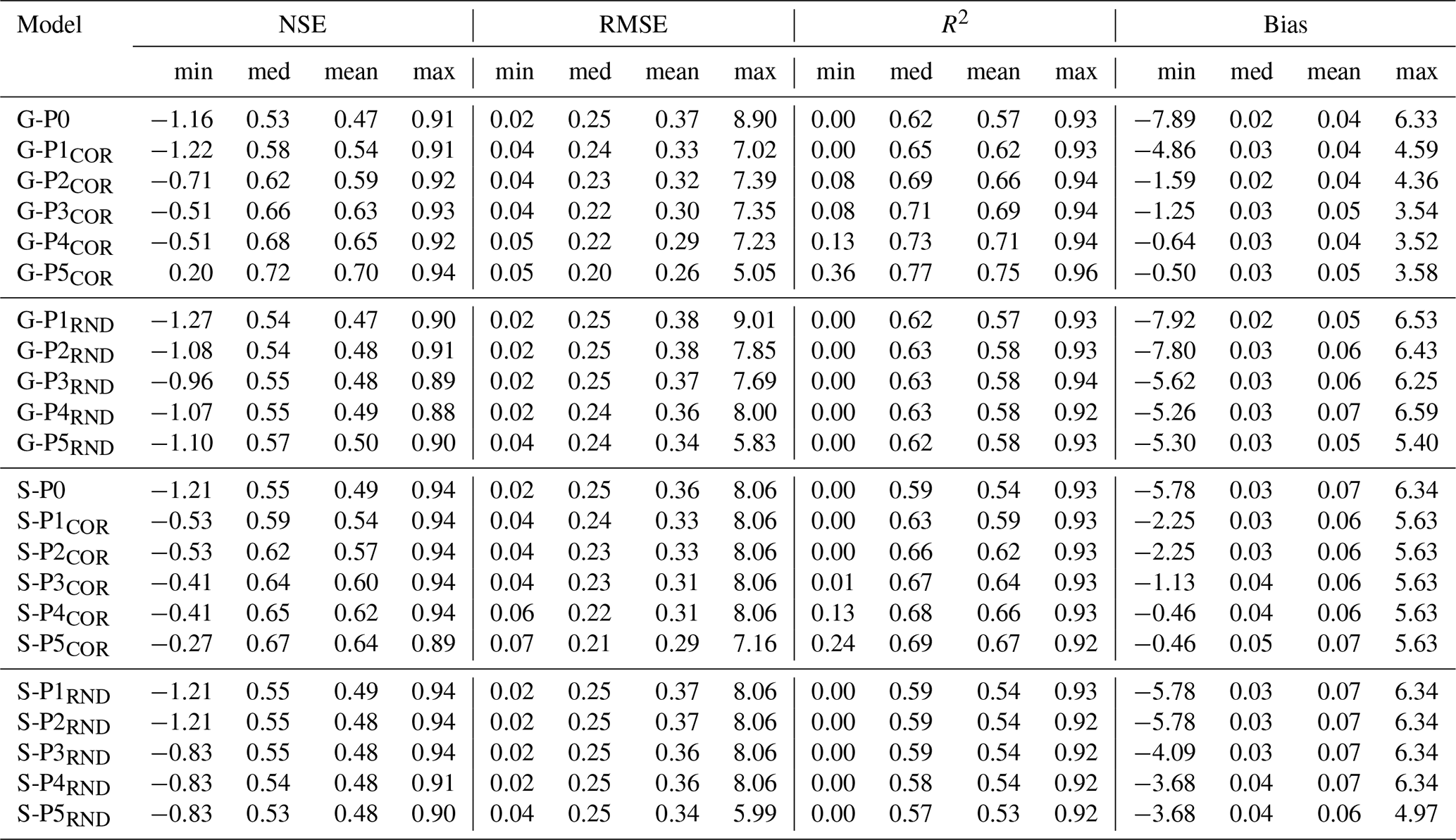
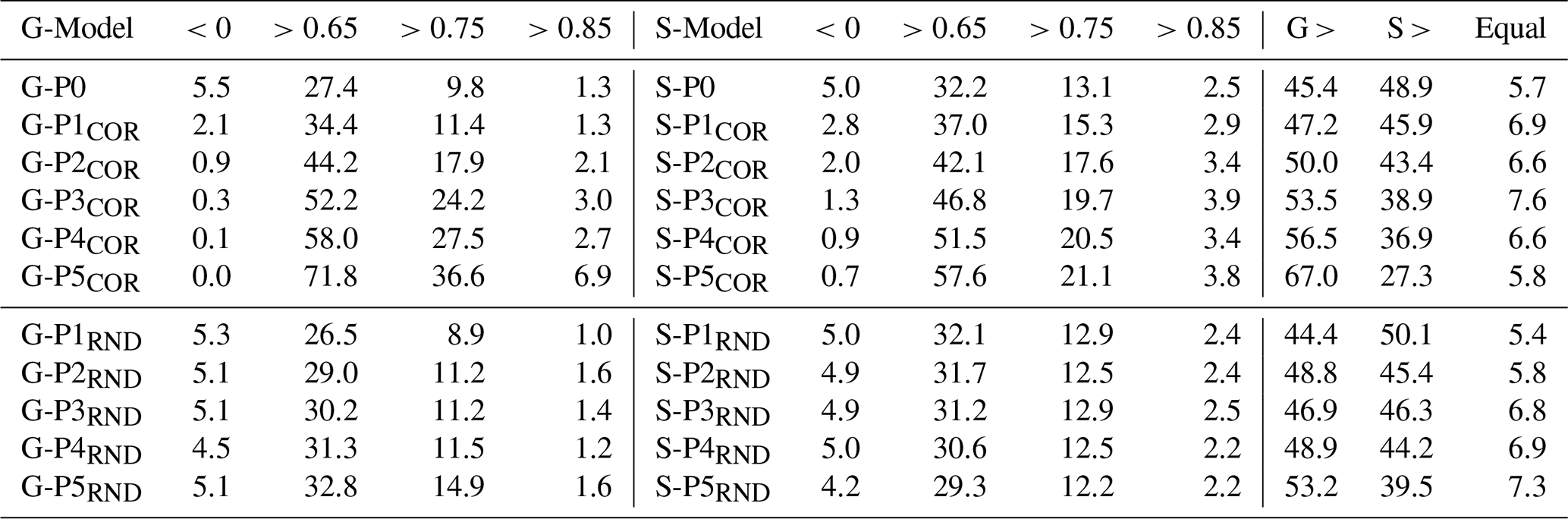
The pairwise comparison in Table 2 confirms these trade-offs: G-P0 outperforms S-P0 at 45.4 % of wells, underperforms at 48.9 %, and performs equally (within ±0.01 NSE) at 5.7 %. Thus, both model types perform broadly comparably, reflecting the balance between generalization and local adaptation.

Table 2 Summary of model performance across correlation- and randomly reduced training subsets. Left columns show NSE-based performance groups for global models (G), middle columns the corresponding results for local single-well models (S) trained on the same well subsets. Right columns report the share of wells for which global models perform better, worse, or equally (±0.01 NSE) compared to their local counterparts.

The cumulative NSE curves (Fig. 3a, lower) show that performance differences vary across the NSE spectrum: S-P0 is slightly better at the very low end (NSE < 0.05), G-P0 performs better from 0.05 to 0.325, both are similar between 0.325 and 0.425, and S-P0 is more favorable in the mid-to-high NSE range.

To test whether these local differences are spatially structured, Fig. 1 maps per-well $\mathrm{\Delta }\mathrm{NSE}={\mathrm{NSE}}_{\mathrm{G}}-{\mathrm{NSE}}_{\mathrm{S}}$ and summarizes local spatial association using a LISA analysis. Although ΔNSE is close to zero on average (P0: mean $=-\mathrm{0.012}$, median $=-\mathrm{0.006}$, share of wells with Δ>0 is 48.7  %), it exhibits significant positive spatial autocorrelation (Global Moran's I=0.322, p=0.001). The LISA results indicate localized clusters of consistently positive or negative ΔNSE as well as spatial contrasts (19.7 % significant at α=0.05), with the most pronounced clustering in hydrogeological region (3) (Upper Rhine Graben including the Mainz Basin and the North Hessian Tertiary), where dense monitoring facilitates the detection of significant local patterns and the patchwork of river-influenced and more regionally coherent dynamics likely contributes to spatially organized model advantages. Overall, this suggests that performance differences are spatially organized in parts of the domain, while remaining non-significant for the majority of wells.

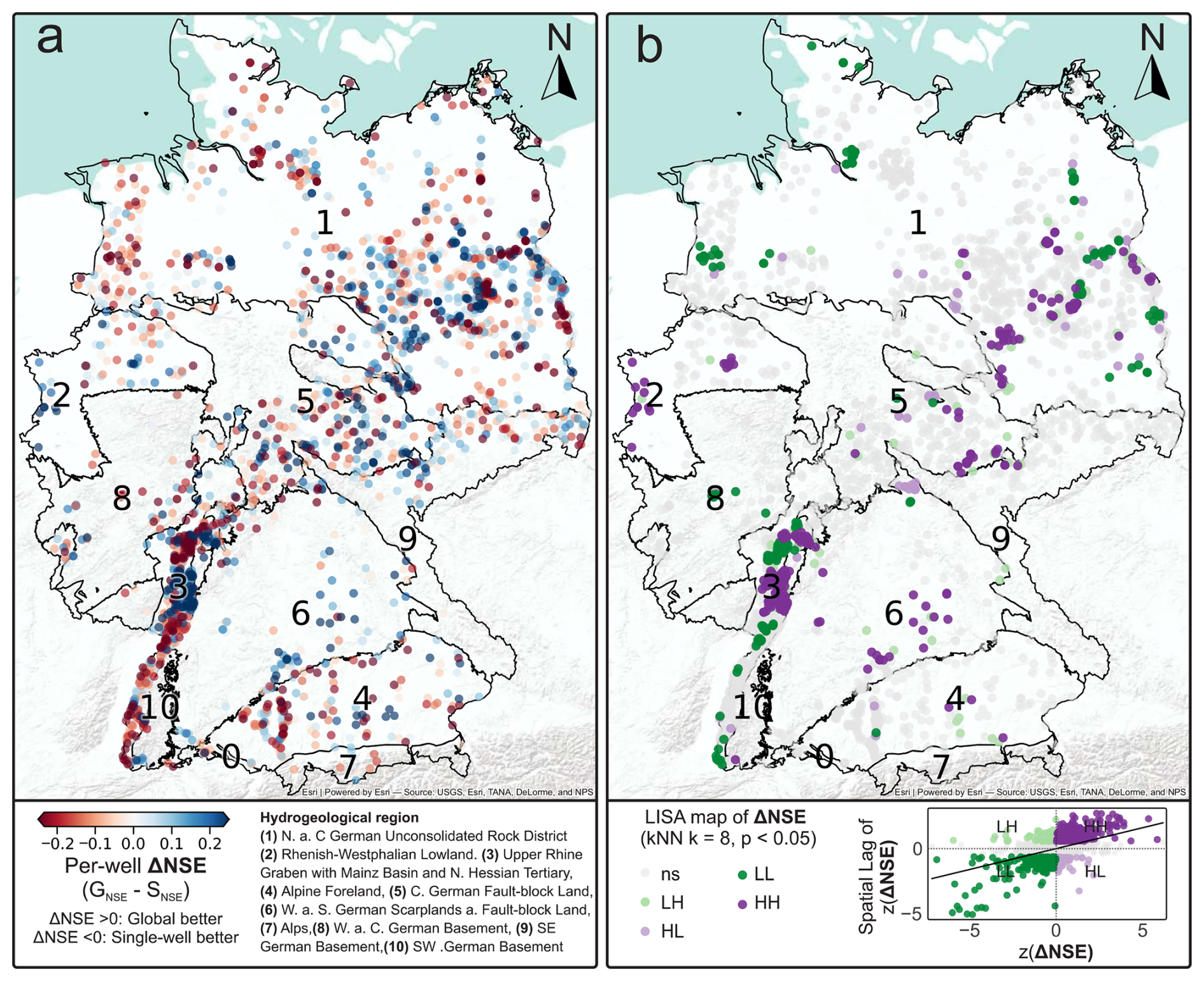
Figure 1 Spatial patterns of per-well performance differences. Spatial patterns of per-well performance differences expressed as $\mathrm{\Delta }\mathrm{NSE}={\mathrm{NSE}}_{\mathrm{G}}-{\mathrm{NSE}}_{\mathrm{S}}$. (a) Pointwise map of ΔNSE across all wells (positive: global model performs better; negative: single-well model performs better). (b) Local Indicators of Spatial Association (LISA) map of ΔNSE based on a k-nearest-neighbor graph (k=8, row-standardized weights; p<0.05), highlighting significant High–High (HH), Low–Low (LL), High–Low (HL), and Low–High (LH) clusters; non-significant locations are marked as ns.

4.2 Influence of the Training Data Basis (RQ ii)

To assess how training data characteristics affect global model performance, we analyze three complementary experiments: (i) sensitivity to training-record length by progressively shortening the available training period in annual steps while keeping the validation and test periods fixed (2008–2012 and 2013–2022), (ii) increasing dynamic similarity through correlation-based well removal, and (iii) reducing training data volume (while maintaining diverse dynamics) through random subsampling.

4.2.1 Training-record length

We additionally tested how sensitive the model comparison is to the length of the available training record. Starting from 1991–2007, we progressively shortened the training period in 1-year steps (removing the earliest years first), while keeping validation (2008–2012) and test (2013–2022) fixed.

Figure 2 summarizes NSE as a function of training-record length for single-well (S) and global (G) models. In (a), median NSE and the 5th–95th percentile band are shown. For long records (approximately 10–17 years), both models exhibit similar medians with strongly overlapping bands. With decreasing training length, S shows a clear drop in median performance and a pronounced widening of the distribution, including negative NSE in the lower tail at short records. In contrast, G remains comparatively stable in median NSE and shows only a modest increase in spread. (b) confirms these patterns in the corresponding density distributions: S progressively broadens and shifts toward lower NSE with shorter records, whereas G stays more concentrated and retains more mass at higher NSE values.

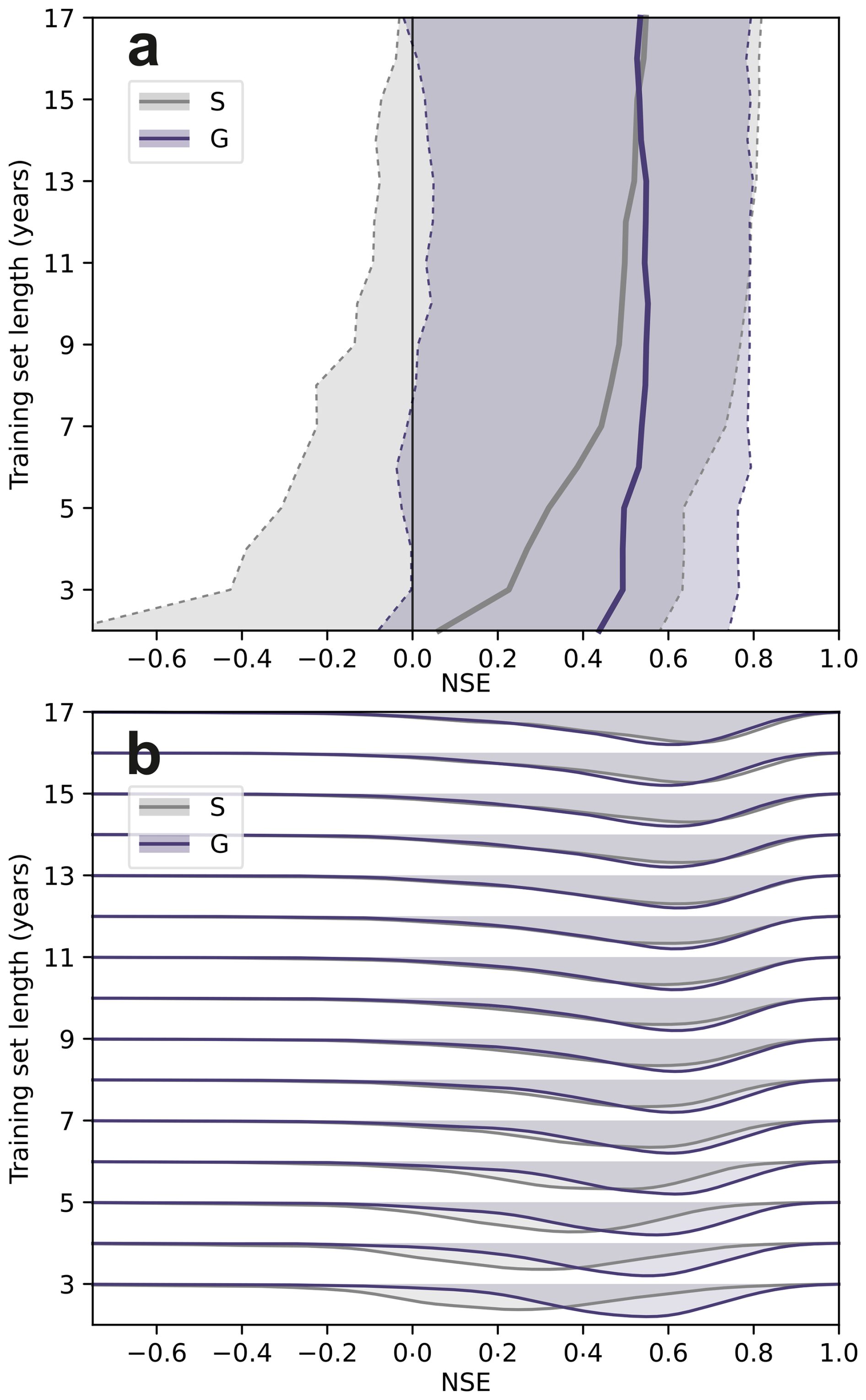
Figure 2 Sensitivity to training-record length. Test-period NSE distributions for single-well (S) and global (G) models as a function of the available training-record length, obtained by progressively truncating the earliest training years in 1-year steps while keeping validation (2008–2012) and test (2013–2022) fixed. (a) Median NSE (solid line) and the 5th–95th percentile range across wells (shaded; dashed bounds); the vertical line marks NSE = 0. (b) Corresponding NSE distributions for each training length shown as overlapping ridgeline density estimates (per-length normalized for visual comparability).

4.2.2 Dynamic Similarity

To investigate how increasing the internal consistency of the training data affects global model performance, we compare the baseline model G-P0 to a series of partitioned models (G-P1_COR to G-P5_COR) trained on increasingly homogeneous subsets. In each step, 500 wells with the lowest average correlation to all other time series were removed to create dynamically more similar training sets.

Figure 3a and Table 1 show that model skill improves consistently with increasing similarity. The share of poorly performing wells (NSE < 0) decreases from 5.5 % (G-P0) to 0.0 % (G-P5_COR), while the proportion of highly accurate wells (NSE > 0.75) increases from 9.8 % to 36.6 %. The mean NSE rises progressively from 0.47 (G-P0) to 0.54 (G-P1_COR), 0.59 (G-P2_COR), 0.63 (G-P3_COR), 0.65 (G-P4_COR), and 0.70 (G-P5_COR). The median NSE shows a similar trend, increasing from 0.53 to 0.58, 0.62, 0.66, 0.68, and finally 0.72.

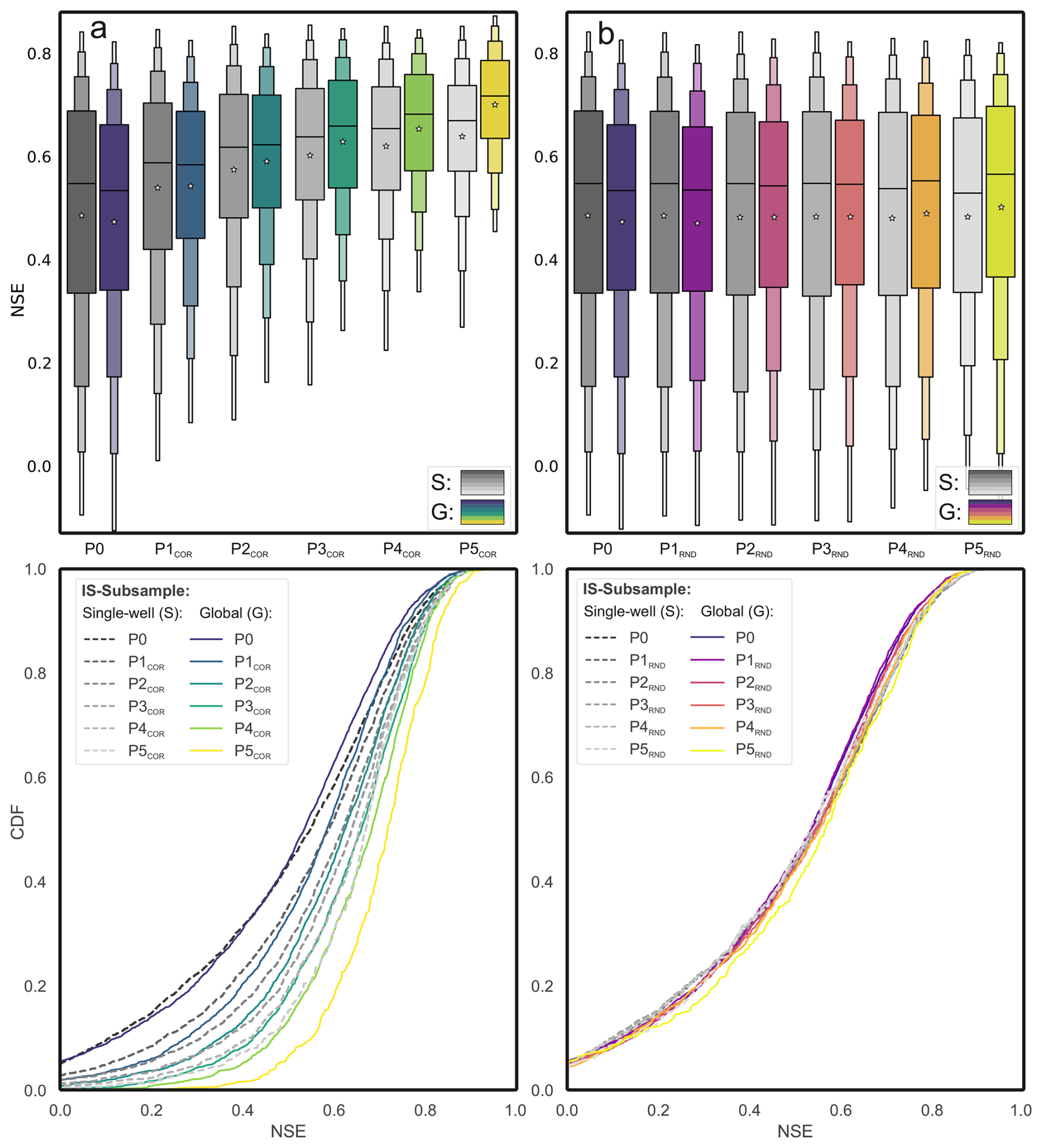
Figure 3 Comparison of single-well and global model performance across generalization stages. (a, b) Distributions of NSE scores (top) and cumulative distribution functions (bottom) for single-well (S) and global models (G-P0–G-P5), based on either correlation-based (a, G-P_COR) or random (b, G-P_RND) well selection. Stages are cumulative subsets of P0 obtained by removing x×500 wells ($n=\mathit{\{}\mathrm{2951},\mathrm{2451},\mathrm{1951},\mathrm{1451},\mathrm{951},\mathrm{451}\mathit{\}}$ for P0–P5). Each global model is compared to S models evaluated on the same subset, illustrating shifts in performance distributions with increasing training data homogeneity (a) or quantity (b).

Compared to the corresponding single-well models, global models benefit more strongly from this increased similarity. At stage P5_COR, the median NSE of the global model (0.72) exceeds that of the local model (0.67), and the proportion of wells with NSE > 0.75 is nearly twice as high (36.6 % vs. 21.1 %) (Table 1). Moreover, the share of wells where the global model outperforms its single-well counterpart increases from 45.4 % (G-P0) to 67.0 % (G-P5_COR) (Table 2).

This trend is further illustrated in Fig. 4a, which plots global versus local NSE scores across wells for each partition stage. While G-P0 shows many points below the 1:1 line, later stages exhibit a progressive upward shift toward and beyond the diagonal. This indicates that, as training sets become more homogeneous, global models increasingly match or exceed local model performance at individual wells. The point cloud also narrows at higher stages (e.g., P4, P5), reflecting more stable and consistent predictions across sites.

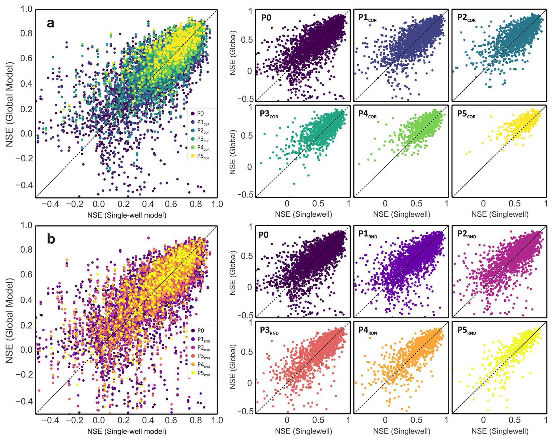
Figure 4 Comparison of global and single-well model performance at the well level. Panels (a) and (b) show NSE values of global models (G-Px) plotted against their corresponding single-well models (S-Px) for each monitoring well. Panel (a) includes models trained on dynamically similar subsets (G-P_COR), and panel (b) shows models trained on randomly selected subsets (G-P_RND). Colored points indicate generalization stages (P0–P5; cumulative removal of x×500 wells from P0); therefore, the set of wells varies across stages. Right-hand subplots display the same data disaggregated by stage. Points above the 1:1 line mark wells where the global model outperforms its single-well counterpart.

Figure 5a highlights the strong relationship between time series representativeness, quantified as the mean absolute correlation to all other training wells, and model performance. Wells with low representativeness tend to exhibit higher error variance and more frequent underperformance, especially at early stages. From stage P3 onward, a clear threshold emerges around a representativeness value of 0.45, above which consistently high NSE values are achieved. This underscores the central role of dynamic similarity in improving global model skill and reliability.

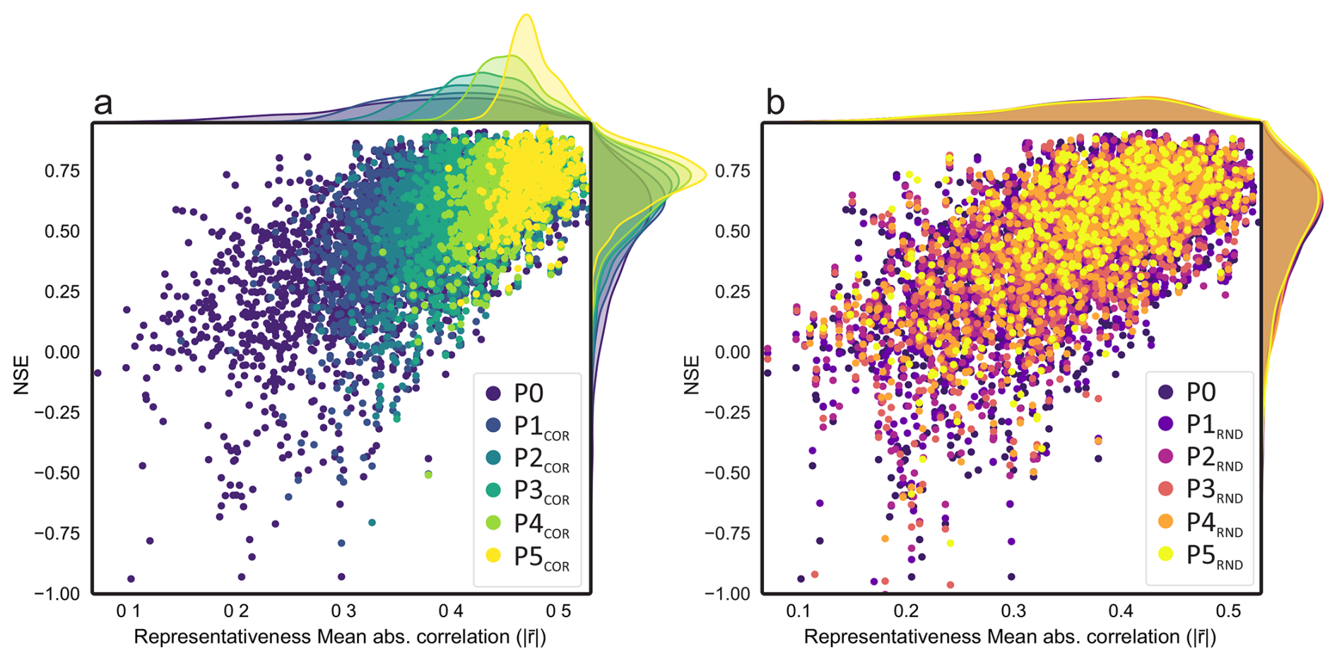
Figure 5 Relationship between time series representativeness and model performance. NSE scores of global models are plotted against the representativeness of each well, defined as the mean absolute correlation with all other training wells. Panel (a) shows results for correlation-based removal (P1–P5_COR), and panel (b) for random removal (P1–P5_RND). Stages are cumulative subsets of P0 obtained by removing x×500 wells. Densities along the top axis indicate the distribution of representativeness across generalization stages (P0–P5). Model performance increases with higher representativeness, particularly under the COR setting, where wells with atypical dynamics are systematically excluded.

A qualitative view of these relationships is provided in Fig. B1, which displays min–max normalized groundwater level time series for every 20th well, sorted by representativeness, along with the difference in predictive performance (ΔNSE) between single-well and best-performing global models.

Finally, Fig. 6 complements the distributional NSE analysis by quantifying how model updates translate into performance changes across stages. Panel (a) compares successive-stage deltas (ΔNSE between two consecutively retrained global models) evaluated on the wells that remain in both stages (i.e., a stage-dependent test set). Across both strategies, median ΔNSE values stay close to zero (often slightly positive), indicating that retraining on moderately reduced datasets does not systematically deteriorate predictive skill for the wells that remain. A clear contrast, however, is visible in the dispersion of ΔNSE: under correlation-based removal (Px_COR), the distributions tend to become narrower with progressing stages, suggesting more consistent performance changes across wells as the training data are progressively homogenized in terms of dynamics. In other words, removing dynamically atypical wells reduces conflicting learning signals and stabilizes how retraining translates into changes in predictive skill on the remaining wells. Under random removal (Px_RND), the spread of ΔNSE increases as the training set shrinks, reflecting higher sensitivity to which wells are retained and a higher variance in retraining outcomes, including more pronounced negative deltas for a subset of sites.

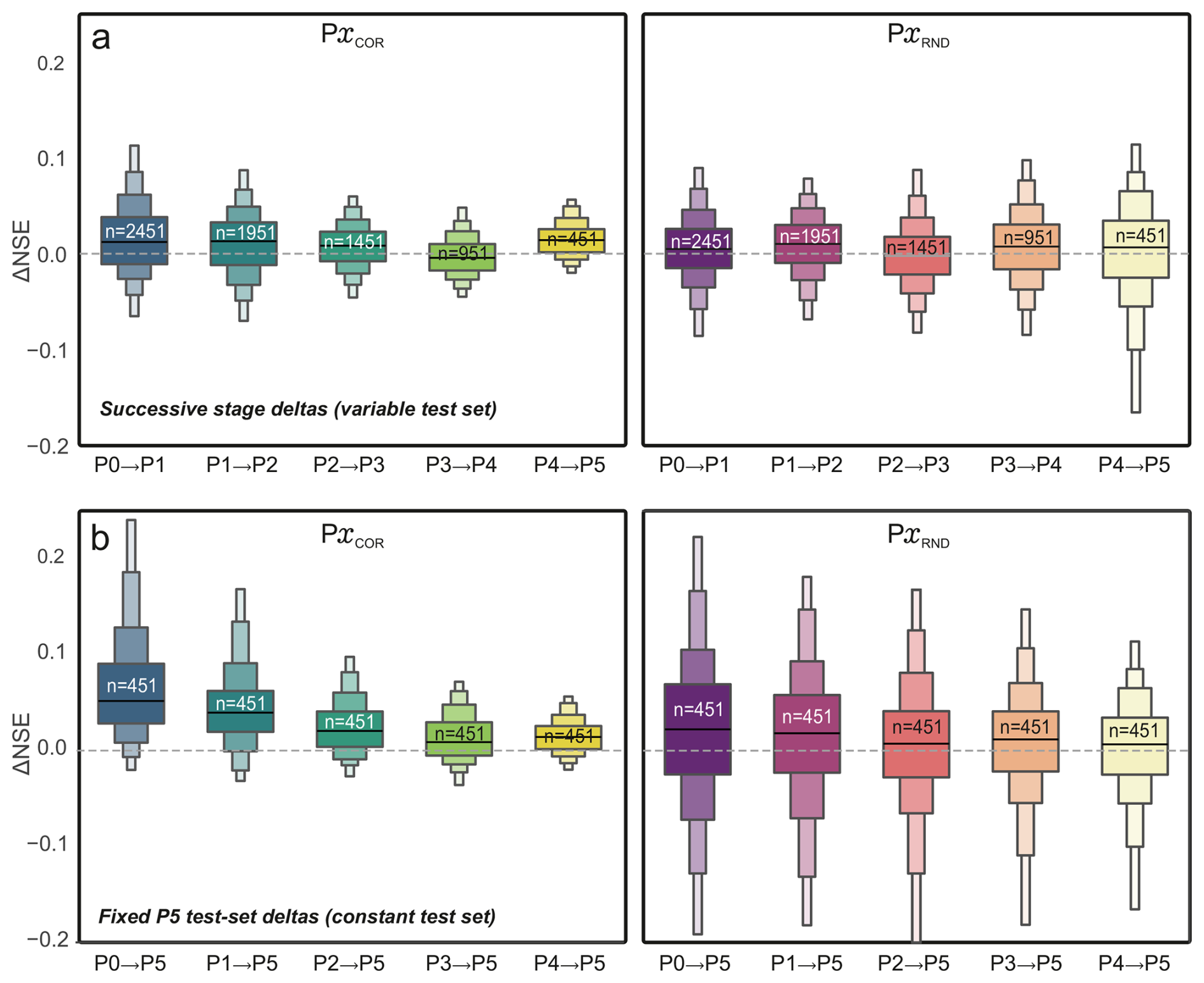
Figure 6 Change in model performance across generalization stages. Distributions of ΔNSE for global models across reduction stages under correlation-based (left; COR) and random (right; RND) well removal. (a) shows successive-stage deltas (e.g., P2 → P3), computed on wells present in both consecutive stages (stage-dependent test set). (b) shows fixed-test-set deltas evaluated on the same P5 wells for all comparisons, quantifying ΔNSE (Px → P5) = NSE (P5) − NSE (Px) (e.g., P2 → P5). Boxes are labeled with the corresponding sample size (n). Across both strategies, median ΔNSE values remain close to zero, indicating no systematic loss of predictive skill with increasing data reduction.

Panel (b) evaluates deltas on a fixed and identical test set, i.e., the wells that constitute the final stage P5 (constant n), thereby isolating training-basis effects from changes in the evaluated well population. For Px_COR, deltas are predominantly positive for early stages and progressively approach zero towards P4 → P5, indicating that the final P5 model achieves systematically higher skill on the representative P5 wells than models trained on less filtered datasets, but that most of this improvement is already realized by intermediate stages (diminishing additional gains thereafter). In contrast, PxRND yields broader, near-zero-centered distributions with substantial positive and negative mass, implying that the final-stage model is not uniformly superior to randomly reduced counterparts on the same P5 wells; rather, gains and losses are site-dependent. Together with Fig. 5, this indicates that the improvements under COR are primarily driven by the targeted exclusion of dynamically atypical wells (i.e., increasing representativeness), rather than by data-volume reduction alone.

4.2.3 Training Set Size

To isolate the effect of training data quantity on global model performance, we conducted a second experiment in which wells were randomly removed from the original training set in steps of 500, resulting in five increasingly reduced datasets (G-P1_RND to G-P5_RND). In contrast to the correlation-based approach, dynamic similarity was not considered here, allowing us to assess whether model skill improves simply with more training data and whether a critical threshold exists.

Despite the substantial reduction in training data, down to just 451 wells in G-P5_RND, global model performance remains remarkably stable. Median NSE values vary only marginally between 0.53 and 0.55, and mean values hover around 0.48 across all stages (Table 1). Similarly, the interquartile range and the overall shape of the NSE distributions (upper part of Fig. 3b) show little variation, and the cumulative distribution curves (lower part of Fig. 3b) remain largely overlapping. These results suggest that increasing training set size alone does not necessarily lead to better model skill. Interestingly, the global model slightly outperforms the corresponding single-well models in the final stages (P4–P5), reflecting a shift toward more dynamically coherent wells. Thus, while random data reduction does not degrade performance, it also does not yield the benefits commonly associated with larger datasets.

This interpretation is further supported by the summary in Table 2, where the share of poorly performing wells remains around 5 %, and the proportion of high-performing wells (NSE > 0.75) increases slightly, from 9.2 % to 14.9 %, despite the lower number of wells. The global model consistently performs as well as or slightly better than the corresponding local models in the final stages (G > S: 53.2 % at P5_RND). While dynamic similarity would be expected to remain constant under random removal, this is not entirely the case for our real-world dataset, as representativeness does not increase continuously but in discrete jumps. At smaller training set sizes, the probability of retaining a more homogeneous subset therefore increases, which can lead to a modest performance gain in later stages. Nevertheless, this improvement is far less pronounced than with correlation-based filtering.

The scatter plots in Fig. 4b further support these findings: in contrast to the correlation-based experiment, there is no clear upward shift of the global model scores across stages. Points remain evenly scattered along the 1:1 line, and the share of wells where the global model outperforms the local one increases only marginally. This visual stability reinforces the notion that model skill is mainly independent of training set size, unless accompanied by improved dynamic similarity.

Figure 5b illustrates that, even under random well removal, wells with high representativeness (mean absolute correlation $\left|\stackrel{\mathrm{‾}}{r}\right|>\mathrm{0.45}$) consistently yield high NSE scores across all stages. However, unlike the correlation-based approach, the representativeness distribution remains broad, and wells with atypical dynamics persist throughout all subsets. As a result, no clear performance threshold emerges and overall skill remains largely stable. There is, however, a slight performance increase of G-P_RND across stages, although this effect is modest compared to the gains observed with correlation-based filtering. This small improvement reflects a property of our dataset: representativeness does not increase gradually but in discrete steps, which increases the likelihood that smaller, randomly selected subsets contain more dynamically homogeneous wells. These findings highlight the importance of dynamic similarity rather than dataset size for achieving high predictive skill.

The ΔNSE diagnostics in Fig. 6 further support this interpretation for random removal. In the stage-dependent comparison (panel a), median deltas remain close to zero while the spread increases towards later stages, indicating that retraining outcomes become more variable as the training set shrinks, without a systematic net improvement. Importantly, this conclusion also holds when controlling for the evaluated wells (panel b; fixed P5 test set): the ΔNSE distributions remain broad and centered near zero, with substantial positive and negative mass. Thus, random reduction does not consistently steer the training basis towards higher representativeness; instead, performance changes on the same wells are largely site-dependent, reinforcing that dynamic similarity – not training set size per se – is the dominant driver of systematic performance gains.

4.3 Prediction of Extreme Events (RQ iii)

To assess model performance under extrapolative conditions, we evaluated predictions for groundwater levels (GWLs) beyond the typical range observed during training. For each well, low extremes were defined as values in the test period below the 1st percentile of its training distribution, and high extremes as values above the 99th percentile. This site-specific percentile approach ensures that extremes are identified relative to each well’s training history, while avoiding dependence on absolute thresholds.

Figure 7 summarizes RMSE distributions for all extrapolated values (top), low extremes (middle), and high extremes (bottom), using both correlation-based and random partitioning. Across all stages, global models do not show improved predictive skill over single-well models. For low extremes, errors are slightly higher for global models at every stage, suggesting that dynamics associated with exceptionally low GWLs are underrepresented in the training sets. For high extremes, both model types perform similarly, with neither showing a consistent advantage.

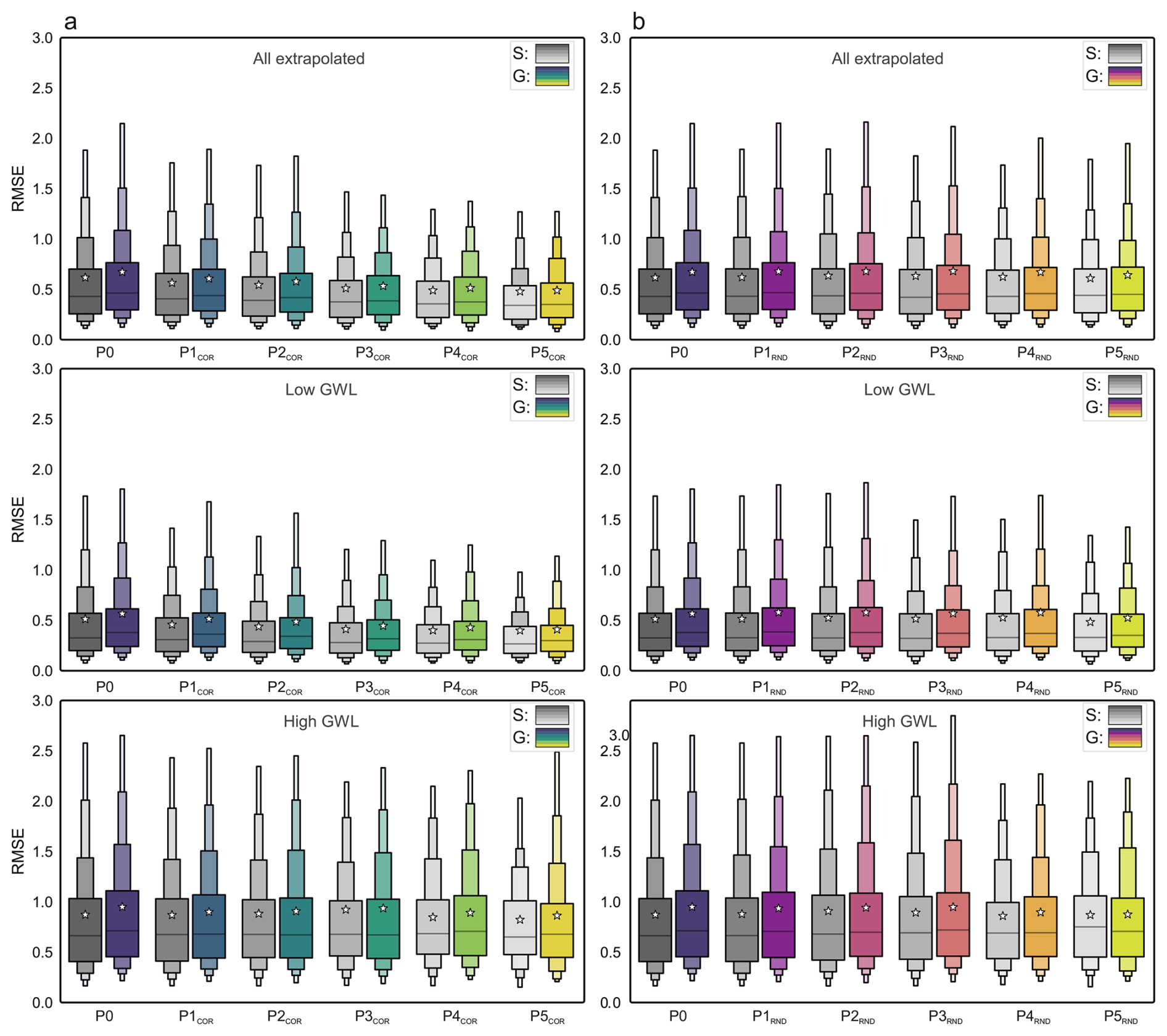
Figure 7 Model performance under extrapolated conditions. Boxplots of RMSE for single-well (S) and global (G) models across generalization stages (P0–P5). Panel (a) shows correlation-based stages (G-P_COR) and panel (b) random stages (G-P_RND). Results are computed for extrapolated time steps only (top) and split into low (middle) and high (bottom) groundwater-level extrapolations.

The stability of error distributions across increasing training set homogeneity or size indicates that, in groundwater systems, larger or more homogeneous datasets do not automatically enhance the prediction of extremes. A plausible explanation is that extreme events often depend on site-specific factors such as fine-scale geology, localized abstraction, or land use, which are not fully captured by the available static site descriptors. Without sufficiently informative descriptors, the transfer of extreme-event knowledge between sites is limited, and events not directly inferable from the dynamic meteorological inputs remain difficult to predict. This reflects a general constraint of current large-scale groundwater datasets rather than a shortcoming of the modeling approach itself.

4.4 Out-of-Sample Spatial Prediction (RQ iv)

To evaluate the spatial transferability of global models, we assessed their performance on monitoring wells deliberately excluded from model calibration. This simulates predictions at sites without prior training data, while observations remain available for evaluation. Out-of-sample (OOS) subsets were defined using the partitioning strategies introduced in Sect. 3.1, i.e., correlation-based removal of dynamically dissimilar wells and random exclusion. Model performance at these OOS sites was compared to that of single-well models trained individually on each target well (in-sample reference). Figure 8 summarizes the resulting differences in predictive skill.

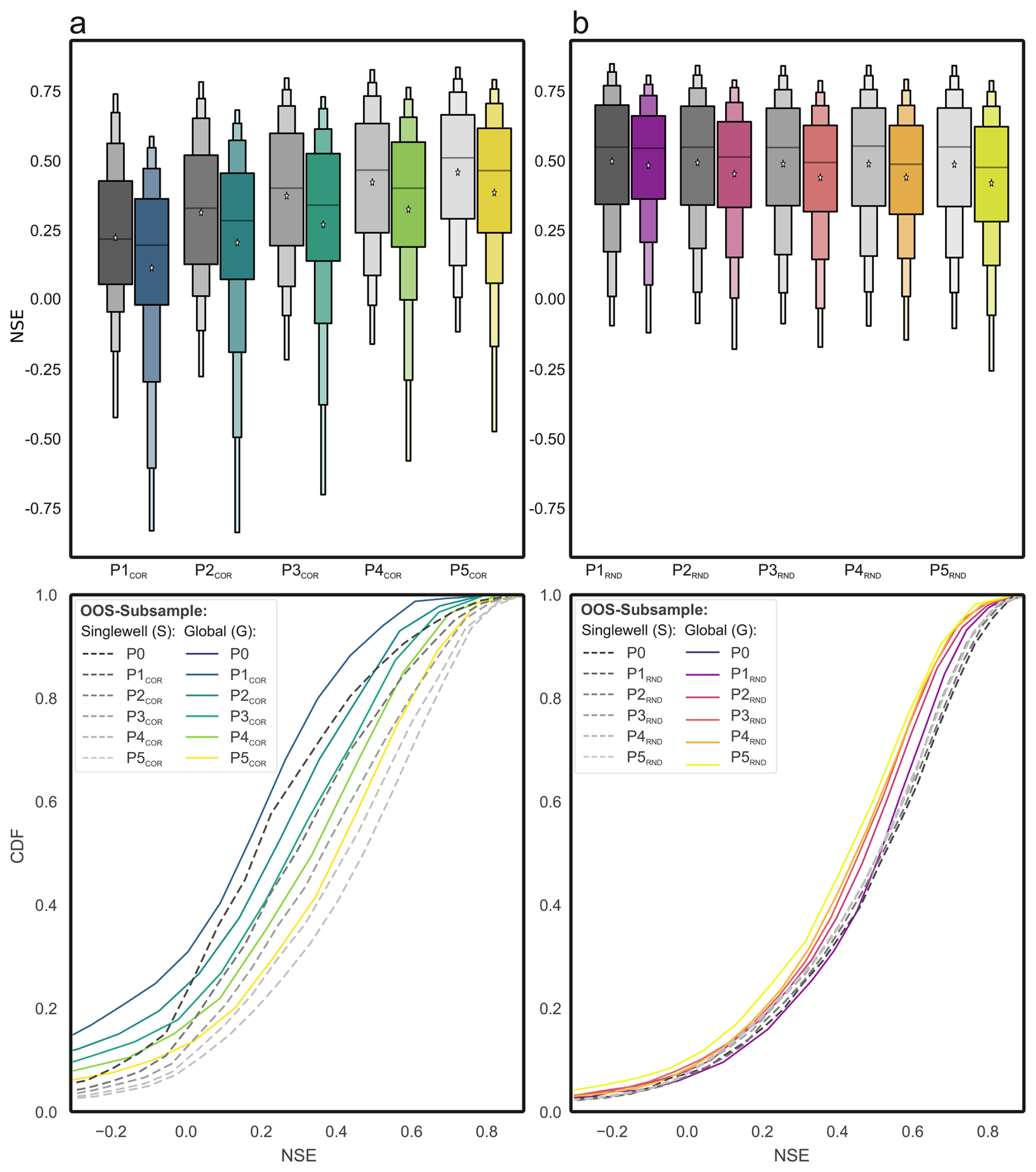
Figure 8 Comparison of single-well and global model performance across generalization stages (out-of-sample wells). Boxplots (top) and cumulative distribution functions (CDFs, bottom) of NSE for global (G) and single-well (S) models evaluated on the held-out wells of stages P1–P5. Panel (a) shows correlation-based exclusion (G-P_COR) and panel (b) random exclusion (G-P_RND). Global models are trained without the held-out wells (spatial transfer), whereas S models provide a site-specific in-sample baseline for the same wells.

At stage P_x, the global model is trained on the remaining wells of that stage and evaluated on the wells excluded up to that stage (cumulative OOS target set). Hence, the OOS test set varies across stages (increasing from 500 to 2500 wells), and cross-stage comparisons should be interpreted as transfer to different target populations rather than a like-for-like evaluation on a fixed test set.

4.4.1 OOS Based on Dynamic Similarity

The upper panel of Fig. 8a summarizes performance for wells excluded due to dynamic dissimilarity. Global models consistently underperform single-well models across all stages, reflecting the difficulty of transferring learned dynamics to sites with low similarity to the training data. In early stages, where the excluded wells are most atypical, the performance deficits are largest. As stages progress, the cumulative OOS target set contains an increasing share of wells that are less dissimilar to the remaining training subset, and global model performance improves accordingly. At the same time, the training base shrinks with progressing stages, which limits the extent of these gains.

Despite the rightward shift of the global distributions, the performance gap to single-well models remains substantial across stages. This suggests that global models, even when trained on dynamically more consistent subsets, often lack the site-specificity needed to match locally trained models at excluded wells. Moreover, the global predictions show more extreme low-NSE outcomes in early stages, indicating that highly dissimilar targets increase the risk of severe model failure.

The lower panel of Fig. 8a shows the cumulative distribution of NSE values for the OOS wells. Across all stages, the curves for the global models lie below those of the single-well models, confirming their overall weaker performance. While the global curves shift slightly rightward with increasing stage, the separation persists across much of the NSE range, indicating that the deficit is not confined to a small subset of wells but affects a broad set of targets.

4.4.2 OOS Random Based

Under random partitioning, wells are excluded from training regardless of dynamic similarity. Consequently, the OOS target set grows from 500 to 2500 wells across stages, while the number of training wells decreases from 2451 to 451. Figure 8b summarizes the results.

The upper part of Fig. 8b shows the NSE distributions for global and single-well models across stages. Global models are, on average, slightly less accurate, but the differences remain small and the distributions are largely stable across stages. Extreme low-NSE outliers are rare, suggesting that random data removal does not induce systematic prediction failures.

The lower part of Fig. 8b displays the cumulative NSE distributions for all OOS wells. Global and single-well curves are closely aligned across stages, confirming broadly similar predictive skill under random exclusion, with a small tendency toward underperformance of the global models. These results emphasize that global models can generalize reasonably well when the excluded targets are not systematically dissimilar, but they do not gain a clear advantage over locally specialized models in this setting.

5 Discussion

5.1 Comparison with previous studies

Our findings provide mixed support for earlier results from deep learning applications in hydrology and hydrogeology. In line with studies in streamflow modeling (Kratzert et al., 2019b, 2024; Martel et al., 2025), we find that global models can achieve predictive skill comparable to or exceeding that of local models when trained on large dynamically homogeneous datasets. This confirms the general advantage of cross-site learning in environments where system dynamics are similar, as also observed in other partitioning approaches (Chidepudi et al., 2025; Zhou et al., 2024; Clark et al., 2022). More generally, multi-site training can be attractive because it consolidates model development into a single network-level model (instead of thousands of per-well calibrations) and, in principle, enlarges the training envelope by exposing the model to a broader range of hydro-climatic situations and response regimes. This is often discussed as a pathway to improved robustness and information sharing, particularly for sites with limited local data.

When the available training history is progressively shortened while validation and test remain fixed, single-well model performance deteriorates more strongly and becomes more variable, whereas the global model remains comparatively stable across record lengths. This pattern is consistent with the notion that local deep-learning models require sufficiently long site records to reach their full potential, while global training can partially compensate limited local information via cross-site learning (Wunsch et al., 2021; Ma et al., 2021). In other words, even if global models do not provide a systematic advantage under heterogeneous conditions for long records, their relative robustness under shorter records supports the relevance of multi-site learning for applications where monitoring histories are limited.

However, while global models have often shown clear advantages for streamflow applications (Kratzert et al., 2021; Lees et al., 2022), though not without recent dissenting findings (Tran et al., 2025), our results for groundwater level prediction reveal no overall advantage under heterogeneous conditions. This echoes the broader debate that “global-model superiority” is not guaranteed: even in hydrology, global models can underperform local ones when local dynamics are highly site-specific and when local data quality or representativeness exceeds what the shared feature space can explain.

This difference is likely related to the broader diversity and high small-scale variability of groundwater system dynamics, ranging from highly responsive karst aquifers to inertial systems in low-permeability sediments. Unlike many surface water catchments, groundwater dynamics can differ markedly even over short distances. Nearby wells may share similar static feature values (e.g., geology, land use) yet exhibit distinct responses due to fine-scale geological differences, flow paths, or localized abstraction.

Under such conditions, a global model may still learn a broad range of dynamics present in the training set but (because the available static site descriptors are not sufficiently informative to uniquely identify the controlling local conditions) cannot reliably assign the correct dynamic regime to a specific well. This is the case even though our benchmark includes a comparatively rich set of >50 time-invariant static attributes (hydrogeology, topography, soils, land use) and intentionally excludes groundwater time-series statistics. As a result, the model tends to average across similar but not identical behaviors, which reduces site-specific accuracy under heterogeneous conditions. This highlights a key trade-off between global and local strategies: global models emphasize breadth and generalization, whereas single-well models emphasize local precision and are less prone to “smoothing” unique site behavior into a dominant average regime. In settings with strong local controls that are not fully observable from static descriptors, local models can remain highly competitive – especially when long, high-quality site records are available. This mechanism is consistent with the strong empirical link between time-series representativeness and model skill observed in our experiments: wells whose dynamics are well represented by the remaining training pool (high mean absolute correlation) are systematically easier to predict, whereas atypical wells show substantially higher error variance. Targeted correlation-based filtering shifts the training data towards this representative regime and thereby reduces conflicting learning signals. Consistent with the concerns raised by Heudorfer et al. (2024), this reflects a broader limitation of large-scale groundwater applications, where even rich static descriptors may not fully capture fine-scale controls such as local flow paths or abstraction. While dynamic similarity may correlate with some static attributes, our filtering is purely time-series based and not spatially constrained; therefore, increasing dynamic similarity does not necessarily imply a strong homogenization of static features.

Finally, our partitioning experiments confirm the robustness benefits reported in other hydrological contexts (Chidepudi et al., 2025; Zhou et al., 2024): grouping wells with similar dynamics before training significantly improved the performance of global models, even with fewer training wells. Notably, the ΔNSE diagnostics further indicate that these gains are not merely a consequence of evaluating on an increasingly “easier” subset: when assessed on a fixed well set (the final P5 wells), correlation-based reduction yields predominantly positive performance differences relative to earlier stages and converges towards zero in later stages, whereas random reduction remains broadly centered around zero with substantial site-dependent gains and losses. Together, these results reinforce the broader conclusion from the literature that data homogeneity, whether achieved via targeted filtering or clustering, can be more important for generalization skill than sheer dataset size. In groundwater modeling, dynamic similarity therefore often outweighs data quantity as a determinant of global model skill. In this sense, partitioned (or clustered) global models can be viewed as a pragmatic middle ground: they retain some benefits of information sharing within dynamically coherent subgroups while reducing the risk that strongly dissimilar wells impose conflicting learning signals that hamper site-specific accuracy.

5.1.1 Sensitivity to model choice and scope

Our comparison is based on the benchmark architectures and training protocol introduced in Ohmer et al. (2026) and was designed to isolate the effects of training strategy and training-data composition under fixed model settings; architecture optimization was not the primary objective of this study. Different model classes (e.g., attention-based sequence models or graph-enhanced architectures) may shift absolute performance levels of both local and global approaches, especially if they improve entity awareness or exploit cross-site relations more explicitly. However, we expect the central qualitative patterns reported here to be comparatively robust because all partitioning stages were evaluated under identical protocols and the observed differences are primarily driven by training-data heterogeneity and the informativeness of available site descriptors. In particular, sequence models such as LSTMs are often expected to benefit from larger training sets, whereas local models can remain competitive when cross-site transfer is impeded by heterogeneous dynamics. Accordingly, architecture choice is likely to influence the magnitude of performance gaps, but is unlikely to overturn the main conclusion that dynamic similarity and informative descriptors are key determinants of successful global groundwater modeling in heterogeneous settings. Beyond architecture choice, we also observe that under correlation-based reduction the dispersion of successive-stage performance changes narrows across stages, suggesting that retraining becomes more stable once conflicting learning signals from dynamically atypical wells are removed; this stabilization is not observed under random subsampling. An additional, practically important axis not addressed in this study is sensitivity to record length, i.e., how model skill changes when only shorter groundwater time series are available. This question is highly relevant for transferability to regions with limited historical coverage but represents a separate experimental dimension from the training-set composition and spatial generalization analyses considered here.

6 Conclusions

This study provides a comprehensive evaluation of globally and locally trained deep learning models for groundwater level forecasting. Using a dataset comprising nearly 3000 monitoring wells across Germany, we systematically assessed model performance across diverse hydrogeological settings and under varying conditions of data availability, dynamic similarity, and extrapolation demands. The analysis was guided by four research questions, each addressing a key aspect of model generalization and applicability. Below, we summarize the main findings in response to each question, placing them in the context of previous hydrological research.

6.1 Are globally trained models generally superior to local (single-well) models?

Not necessarily. Despite being trained on a large and diverse dataset, globally trained models did not show a notable overall advantage over locally optimized single-well models. Local models tend to achieve slightly higher median accuracy and perform better at individual sites, while global models produce more predictions clustered around the central range of performance, suggesting a more stable but less specialized behavior. This pattern is consistent with limited entity awareness under heterogeneous conditions, where even a rich set of time-invariant static attributes (>50 hydrogeological, topographic, soil, and land-use descriptors; no groundwater time-series statistics) may be insufficient to uniquely identify the controlling local processes at each well. Conceptually, this reflects the core trade-off: global models emphasize breadth and potential robustness via information sharing, whereas single-well models emphasize local precision and can better capture unique site-specific behavior when long, high-quality local records are available. These findings align with earlier work in groundwater modeling but contrast with the consistent superiority reported for streamflow, likely reflecting the greater diversity and small-scale variability of groundwater system dynamics. However, when training is restricted to dynamically homogeneous subsets, global models can match or even exceed single-well performance at many sites, highlighting that cross-site learning becomes beneficial once heterogeneity is reduced.

6.2 Does training data quality or quantity matter more for global models?

Training data quality in terms of dynamic similarity is more important than quantity. When the training set is filtered to include only wells with similar temporal dynamics, global model accuracy improves markedly, and performance changes become more consistent across sites. In contrast, random removal of wells (reducing size without regard to similarity) does not yield comparable gains, even when roughly 85 % of wells are removed; any changes remain modest and site-dependent. Importantly, evaluating all stages on a fixed test set (the final P5 wells) confirms that the improvements under correlation-based filtering are not merely a consequence of progressively excluding difficult sites, but reflect a genuine benefit of training on a more dynamically consistent data basis. Thus, for in-sample prediction, structure (dynamic similarity/representativeness) matters more than sheer sample size; simply enlarging the dataset without improving consistency provides little benefit. For in-sample predictions, dynamic similarity is clearly the dominant factor; for out-of-sample predictions, a broader and more diverse training base may, in principle, offer robustness benefits, although this was not a dominant effect in our experiments. Consistent with this, global models were also less sensitive to shorter training histories than single-well models under our benchmark setup.

6.3 Can global models reliably predict extreme groundwater events?

No. In our experiments, neither global nor local models could reliably predict groundwater levels outside the training range. Across all partitioning stages and extrapolation regimes, global models showed slightly higher errors and a tendency to overestimate low values while underestimating high ones, consistent with a structural averaging effect. Neither increasing the amount of training data nor improving dynamic similarity mitigated this issue. A likely reason is that the available static site descriptors (e.g., geology, land use, geomorphology) are not sufficiently informative to provide strong entity awareness and to capture the local controls governing extremes, thereby limiting the transfer of extreme-event knowledge between sites. These descriptors represent the best practical dataset currently available for large-scale groundwater modeling, so this limitation reflects a general constraint of current data availability rather than a shortcoming of the modeling approach itself.

6.4 How well do global models generalize to unseen locations?

Under correlation-based exclusion (i.e., deliberately held-out wells with low dynamic similarity), the global model shows limited spatial generalization and performance drops sharply compared to single-well models, reflecting the difficulty of transferring learned dynamics to dissimilar sites. Across successive stages, the OOS target set expands from the most atypical wells to include progressively less dissimilar sites, which leads to a modest rightward shift in global performance; however, the gap to single-well models remains substantial. In contrast, random exclusion yields broadly similar performance across stages, indicating that generalization is feasible when target wells share representative temporal patterns with the training data, consistent with previous findings that groundwater dynamics are less transferable than streamflow. Importantly, our OOS setup evaluates transfer to wells with available historical observations (needed for well-specific scaling), i.e., a realistic “new well with records but not used for training” setting rather than a fully no-head-data scenario.

In summary, the choice between global and local modeling depends strongly on the intended application. For in-sample prediction at known sites, training on dynamically similar wells (e.g., by partitioning or filtering the dataset based on dynamic similarity) can yield accurate results even with relatively few data, as the remaining wells benefit from increased dynamic similarity and the reduced influence of poorly representative sites. For spatial generalization, a broad and diverse training base may improve robustness, although this effect was modest in our experiments and can come at the cost of predictive precision. From an operational perspective, global models can still be attractive because they provide a single maintainable model for an entire monitoring network and enable weight transfer across sites; however, where the goal is maximal site-specific accuracy (especially for atypical wells), single-well models remain a strong and often preferable option. For groundwater systems, characterized by slow and often indirect responses, sparse measurements, high small-scale variability, and limited entity awareness due to coarse static descriptors, model transferability appears inherently more limited than in surface water applications. This highlights that single-well models remain a strong option, especially when site-specific accuracy is required and local dynamics need to be captured in detail.

Appendix A: Spatial distribution of monitoring wells

Figure A1 shows the geographical distribution of all monitoring wells used in the modeling experiments, as well as their progressive removal across different partitioning stages.

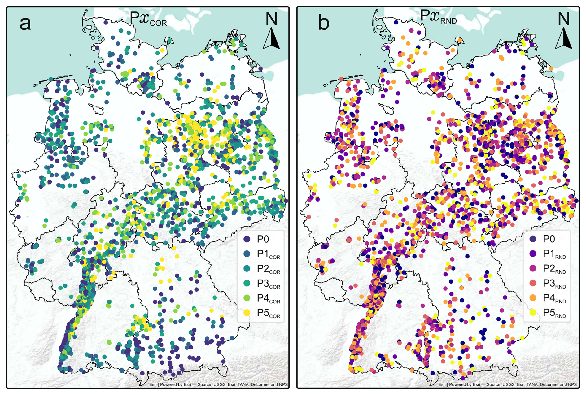
Figure A1 Spatial distribution of groundwater monitoring wells used in this study. The panels distinguish between correlation-based (P_COR, a) and random (G-P_RND, b) data removal scenarios across six stages (P0–P5). Each stage represents a progressive reduction of the training data set, either by removing wells with low dynamic similarity (P_COR) or through random subsampling (G-P_RND). The map highlights how spatial coverage changes with increasing data reduction

Appendix B: Stacked groundwater level time series with representativeness and performance difference

Figure B1 shows min–max normalized groundwater level time series for every 20th monitoring well (from the second-highest representativeness rank), ordered by representativeness.

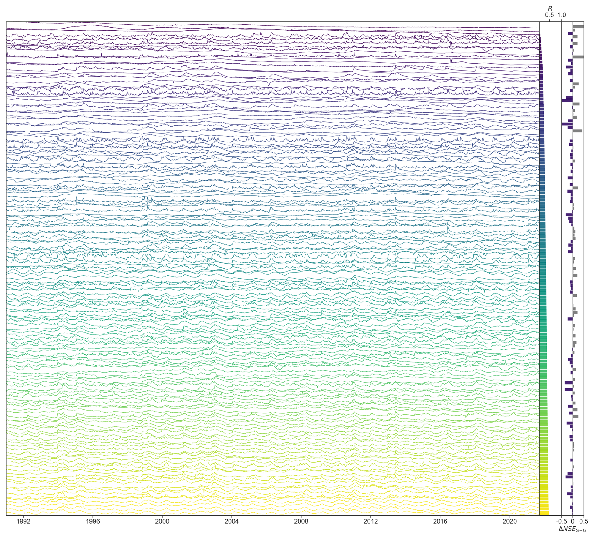
Figure B1 Stacked groundwater level (GWL) time series (min–max normalized) by representativeness. Left: time series color-coded by representativeness (R); middle: bars of R; right: ΔNSE = NSE_S − NSE_G, clipped to $[-\mathrm{0.5},\mathrm{0.5}]$ (dark gray = S better, blue = G better).