A GNN routing module is all you need for LSTM Rainfall–Runoff models

Rainfall–Runoff (R–R) modeling is crucial for hydrological forecasting and water resource management, yet traditional deep learning approaches, such as Long Short-Term Memory (LSTM) networks, often overlook explicit runoff routing, leading to inaccuracies in complex river basins. This study introduces a novel LSTM-Graph Neural Network (GNN) framework that integrates LSTM for local runoff generation with GNN for spatial flow routing, leveraging river network topology as a directed graph. Applied to the Upper Danube River Basin using the LamaH-CE dataset (1987–2017), the model partitions the basin into 530 subbasins and evaluates four GNN architectures: Graph Convolutional Network (GCN), Graph Attention Network (GAT), Graph SAmple and aggreGatE (GraphSAGE), and Chebyshev Spectral Graph Convolutional Network (ChebNet). Results demonstrate that all LSTM-GNN architectures outperform the baseline LSTM, with LSTM-GAT achieving the highest performance (mean NSE = 0.61, KGE = 0.65, Correlation Coefficient = 0.84, RMSE reduction of ∼ 35 %). Improvements are most evident in downstream stations with high connectivity and large contributing areas, where adaptive attention in GAT effectively captures heterogeneous upstream influences. These findings underscore the potential of GNN-based approaches for large-scale, spatially aware hydrological modelling and provide a foundation for future applications in flood forecasting and climate adaptation.

1 Introduction

Rainfall–Runoff (R–R) modelling plays a fundamental role in hydrological science, enabling the prediction of how precipitation transforms into streamflow (Beven, 2012). This predictive capability is essential for a range of applications, including flood forecasting, water resource management, and environmental protection (Hunt et al., 2022). Over the past decades, R–R modelling has advanced through the development of physics-based hydrological models, particularly conceptual and distributed models (Clark et al., 2015). These advances have been supported by improvements in hydrological data availability and computational power (Zhang et al., 2025). Typically, R–R models comprise two core components: runoff generation and runoff routing. Runoff generation refers to the partitioning of rainfall into surface runoff or subsurface flow, while runoff routing represents the transport and temporal distribution of this water through river networks (Beven, 2012). Developing these physical models often requires extensive parameterization and iterative calibration. This challenge is compounded by high-resolution versions, which demand significant data handling. Furthermore, the transferability of such models remains a challenge, as models calibrated for one catchment often perform poorly in ungauged or data-scarce basins (Arsenault et al., 2023).

Recent reviews indicate a notable shift from purely physics-based models towards data-driven approaches, especially deep learning (DL) models (Tripathy and Mishra, 2024). This shift is driven by the increasing availability of streamflow and meteorological datasets. Among these DL methods, the Long Short-Term Memory (LSTM) neural network has gained widespread adoption due to its effectiveness in capturing complex temporal dependencies inherent in hydrological time series (Kratzert et al., 2018; Anderson and Radić, 2022). Most initial DL applications have treated catchments as lumped systems, where meteorological variables are spatially averaged to predict runoff at the outlet. However, with the growing availability of high-resolution spatial datasets (Brocca et al., 2024), more sophisticated deep learning architectures that integrate both spatial and temporal features such as Convolutional Neural Networks (CNNs) combined with LSTMs have emerged (Anderson and Radić, 2022). These models aim to enhance predictive accuracy by leveraging spatial patterns alongside temporal sequences (Li et al., 2023).

Despite these advancements, these deep learning approaches focus solely on runoff generation and do not explicitly model the runoff routing component (Wang et al., 2024). Including runoff routing is crucial because it accounts for flow delays, attenuation, and connectivity within river systems. Neglecting routing can lead to significant inaccuracies, such as overestimation or underestimation of peak flows and misrepresentation of flow dynamics, particularly in large or complex basins (Cortés-Salazar et al., 2023; Baste et al., 2025). For instance, Cortés-Salazar et al. (2023) demonstrated that adding an explicit routing scheme improved the Kling–Gupta efficiency of daily streamflow from 0.64 (without routing) to 0.81 (with the best routing scheme). Some efforts attempt to address this by integrating upstream hydrological information into LSTM models or combining LSTM outputs with physically based routing models (Yu et al., 2024; Yang et al., 2025). While these approaches improve spatial realism, the routing component itself is not inherently learned within the DL framework. This limitation primarily stems from these models' inability to incorporate river network topology in a physically meaningful way.

Graph Neural Networks (GNNs) offer a promising solution to this challenge by explicitly modeling graph-structured data, making them well-suited for representing river network topology (Sun et al., 2021). In the context of hydrology, the river system can be naturally represented as a graph, where nodes correspond to subbasin outlets or gauge locations, and edges, the links that connect these nodes and represent river channels, capture the connectivity of the network. The key strength of GNNs lies in their ability to propagate information across the graph structure through what are known as edges, allowing each node to learn from its upstream and downstream neighbors. This formation flow mimics the physical process of runoff routing, enabling the model to learn spatial dependencies within the river network. Several recent studies have explored GNNs in R–R modeling, treating them as spatiotemporal modules within DL frameworks and highlighting their potential. These models typically combine GNNs with LSTMs or other recurrent architectures to capture both spatial and temporal dynamics. For example, Sun et al. (2022) utilized GNNs to capture physics-based connectivity, demonstrating that graph-based data fusion can serve as an effective surrogate for process-based models. Similarly, Deng et al. (2023) addressed the non-Euclidean structure of river networks using spatiotemporal graph convolutions to capture upstream-downstream correlations. Beyond surface water, Gai et al. (2023) applied GNNs to simulate spring discharge by modeling the complex subsurface connectivity of karst systems. More recently, Wang et al. (2025) showed that optimizing graph topologies, specifically transforming tree-like networks into dense graphs can accelerate flood warnings by capturing long-range dependencies. These models typically combine GNNs with LSTMs or other recurrent architectures to capture spatiotemporal dynamics, with a primary focus on improving representations of spatial variability in inputs or learning latent inter-basin correlations, rather than explicitly modeling the flow-routing process along river networks.

Given the importance of runoff routing, our hypothesis is that incorporating GNNs as a dedicated module for runoff routing will improve runoff prediction. Furthermore, most existing GNN studies in hydrology have been limited to small-scale catchments with relatively few sub-basins (Sun et al., 2022; Gai et al., 2023; Deng et al., 2023). These studies often do not fully exploit the potential of GNNs to represent complex physical routing processes across vast networks. Thus, the explicit use of GNNs for runoff routing in large and complex river basins remains an open and underexplored area in current DL frameworks.

In this study, we aim to address this gap by developing a novel model that integrates LSTM networks with GNNs. The proposed LSTM-GNN architecture leverages the temporal modeling capabilities of LSTMs for each subbasin, while a GNN component explicitly models runoff routing through the river network. The model is applied to predict daily river discharge across the Danube River Basin, a large and topologically complex catchment. The specific objectives of this study are: (1) to evaluate the performance of different GNN architectures such as Graph Convolutional Network (GCN), Graph Attention Network (GAT), Graph SAmple and aggreGatE (GraphSAGE), and Chebyshev Spectral Graph Convolutional Network (ChebNet) as routing modules; and (2) to assess the contribution of the routing component by comparing the proposed LSTM-GNN model against a baseline LSTM model that lacks explicit spatial routing.

2 Study area and dataset

The Upper Danube River Basin (Danube) in Central Europe is chosen as the study area due to its extensive geographical coverage, inherent hydrological complexity, and the rich availability of associated datasets (Fig. 1). It spans about 170 000 km² and crosses or borders nine countries (Austria, Germany, Switzerland, Slovakia, Czech Republic, Hungary, Liechtenstein, Italy, and Slovenia). The basin's terrain ranges from high Alpine headwaters down to lowland plains. The basin experiences a broad range of subbasin-level average annual temperatures from −4.14 to 10.45 °C and receives annual precipitation varying significantly across its subbasins from 650 to 2068 mm (Muñoz-Sabater et al., 2021), reflecting its diverse climatic zones. This strong physiographic and climatic gradient produces a wide diversity of catchment characteristics and highly variable streamflow patterns across the basin.

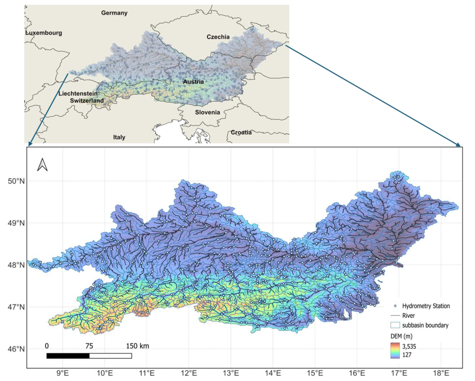
Figure 1 The Upper Danube River Basin (UDRB).

The hydrological dataset for this study comes from LamaH-CE (Large-Sample Data for Hydrology in Central Europe) (Klingler et al., 2021). LamaH-CE provides time series of streamflow and meteorological variables, along with static catchment descriptors for Danube. In total LamaH-CE covers 859 gauged basins over the Danube. We focus on a subset of 530 gauges that have continuous daily streamflow records from 1 January 1987 to 31 December 2017. These 530 subbasins span a very wide range of sizes from a few square kilometers up to over 2500 km² and include diverse topographic, land cover, and hydrologic conditions. The intricate dendritic structure of the Danube river system, along with the dense network of gauging stations, provides an ideal setting to investigate the role of explicit runoff routing in R–R modeling, particularly through graph-based approaches. Three daily meteorological and hydrological variables provided in the LamaH-CE dataset including precipitation, soil moisture (fraction of water in topsoil layer 0 to 100 cm depth), and 2 m air temperature are derived from the ERA5-Land reanalysis (Muñoz-Sabater et al., 2021) and serve as the dynamic inputs for the R–R model. Crucially, these dynamic inputs are spatially averaged over the entire upstream catchment contributing to each gauge, providing a single representative value per basin per day (Klingler et al., 2021). In addition to these time-varying forcings, LamaH-CE offers 59 static catchment attributes for each of the 530 selected subbasins. These static descriptors capture essential physical and environmental features, including topography, climatological norms, hydrological signatures, land cover classifications, vegetation indices, soil characteristics, and geological formations. Similar to the dynamic variables, these static attributes are pre-processed and provided as basin-averaged values.

3 Methodology

We propose a novel LSTM–GNN model to predict the R–R process by jointly capturing local runoff generation and basin-scale flow routing within a unified framework. In contrast to traditional lumped models that treat the catchment as a single unit, our approach partitions the basin into multiple hydrologically connected subbasins, each represented as a node in a graph, with nodes corresponding exclusively to gauged subbasin outlets. At each subbasin, an LSTM unit processes the time series of meteorological inputs including precipitation, soil moisture, and 2 m air temperature to model the temporal evolution of runoff. The output of each LSTM serves as a latent embedding, a vector representation that summarizes the subbasin's runoff response and hydrological state. These node-level embeddings are passed into a GNN, which models spatial interactions across the river network. The river system is represented as a directed graph, where edges reflect downstream flow connections between subbasins. Through messages passing along this graph structure, the GNN propagates and aggregates information from upstream to downstream nodes, enabling explicit modeling of runoff routing and flow accumulation consistent with real-world hydrological connectivity. Importantly, unlike some existing LSTM–GNN models that incorporate historical streamflow as an input (e.g., Deng et al., 2024; Wang et al., 2025), our model excludes streamflow observations. While such data can enhance prediction accuracy in gauged basins, it is inherently unavailable in ungauged regions. By relying solely on meteorological inputs, our framework remains applicable to both gauged and ungauged settings.

As mentioned above, three dynamic variables and 59 static variables are used as input features. All input features are normalized using a positive_robust_log transform for precipitation and streamflow, and min–max scaling [0,1] for other variables, before being used into the models. The historical observed streamflow records serve as the target output (ground truth) for training, validation, and testing. For temporal modeling, a sliding window of 180 d of past data is used as the input sequence, and the model learns to forecast the discharge for the next day. The dataset consists of daily records from 1 January 1987 to 31 December 2017. The dataset was divided into 70 % training and 15 % validation samples selected randomly, and the remaining 15 % (the last part of the time series) was used for testing. To address the inherent class imbalance in hydrological data where extreme discharge events are rare but critically important for flood prediction, we implement a targeted data augmentation strategy. We identified extreme discharge events by selecting the top 2.5 % of maximum discharge values from each subbasin. These events were then augmented by creating four additional copies, increasing their overall representation in the training dataset from 2.5 % to approximately 10 %. This augmentation approach ensures that the model receives sufficient exposure to high-discharge patterns during training, improving its ability to predict flood events while maintaining the overall temporal structure of the time series data. The augmentation is applied only to the training set to prevent data leakage into the validation and testing phases. All models are implemented in PyTorch and trained on a GPU (NVIDIA A100 40GB) to accelerate computation, given the long time series and model complexity.

3.1 Model Architecture

Our proposed model consists of two primary components: an LSTM module for local runoff generation and a GNN module for spatial runoff routing. Each subbasin is represented as a node in the river network and is associated with a local LSTM that processes inputs. Importantly, these subbasin-level LSTMs are not trained independently; instead, all LSTMs share a single set of parameters and are trained jointly as a regional model. The GNN component then enables information exchange between subbasins according to the river network topology, explicitly modeling runoff routing. The entire framework is trained end-to-end across all subbasins simultaneously. The overall structure is visualized in Fig. 2 and described in the following sections.

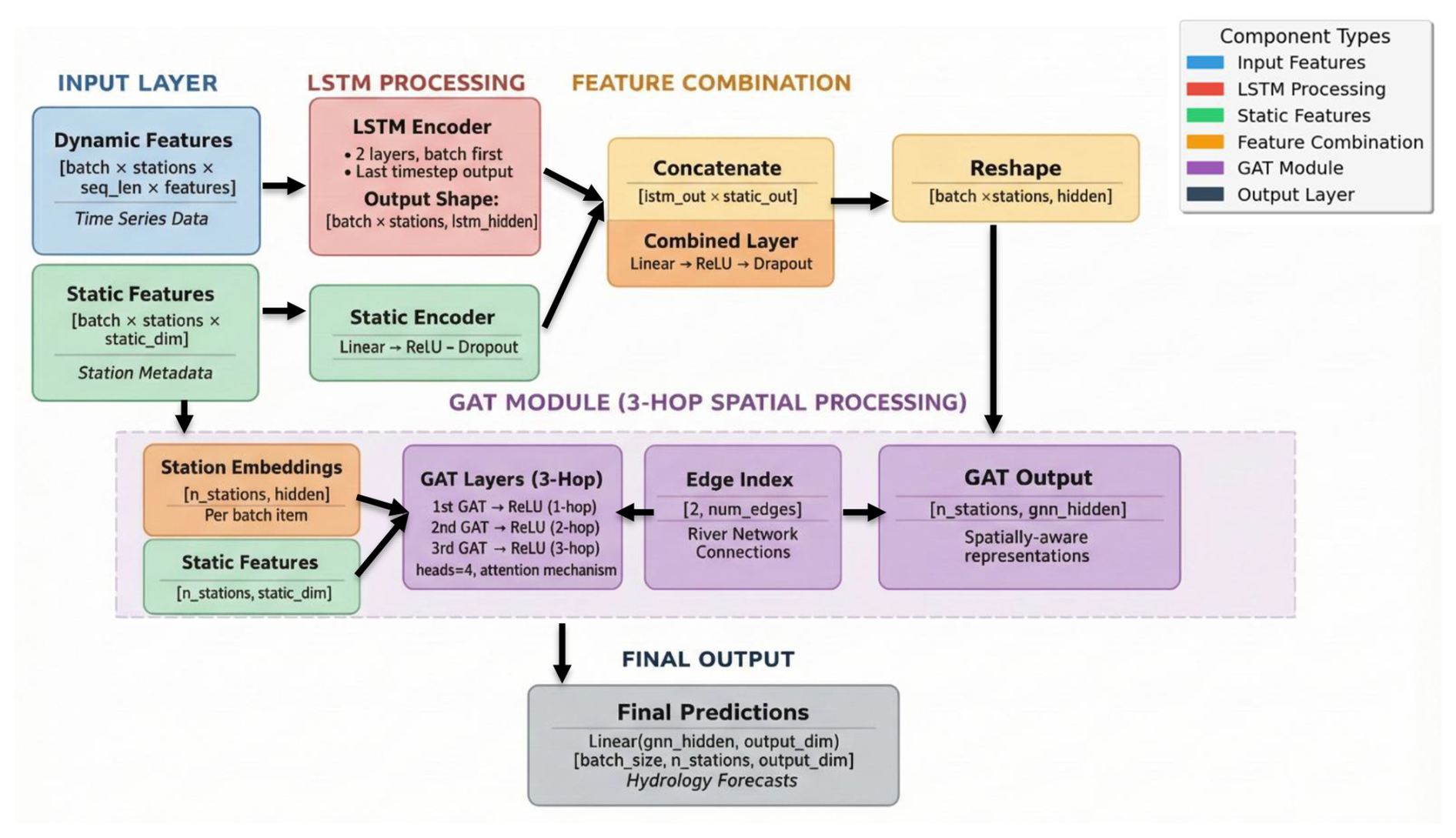
Figure 2 Schematic of the proposed LSTM–GNN model architecture for rainfall–runoff modelling.

3.1.1 LSTM Component: Local Runoff Generation

For each subbasin i, the input sequence is a 180 d time window of meteorological variables:

$$X_i=\mathit{\{}{x}_{i,t-\mathrm{179}},x_{i,t-\mathrm{178}},\mathrm{\dots },x_{i,t}\mathit{\}},x_{i,t}\in R^{d_{\text{dyn}}}$$

where d_dyn=3 (precipitation, temperature, soil moisture). These sequences are fed into a two-layer LSTM to model temporal dependencies:

$$\begin{array}{l}{h}_{i,t}^{\left(\mathrm{0}\right)}=x_{i,t}\\ h_{i,t}^{\left(l\right)}={\text{LSTM}}^{\left(l\right)}\left(h_{i,t-\mathrm{1}}^{\left(l\right)},c_{i,t-\mathrm{1}}^{\left(l\right)},h_{i,t}^{(l-\mathrm{1})}\right),l=\mathrm{1},\mathrm{2}\\ z_i=h_{i,t}^{\left(\mathrm{2}\right)}\end{array}$$

here $h_{i,t}^{\left(l\right)}$ and $c_{i,t}^{\left(l\right)}$ denote the hidden and cell states of layer l, and $z_i\in R^{d_{\text{lstm}}}$ represents the final hidden state (with d^lstm=128) capturing the temporal runoff behaviour of subbasin i. To incorporate physical characteristics, we also use 59 static catchment attributes per subbasin s_i∈R⁵⁹, which are passed through a feedforward encoder with ReLU (Rectified Linear Unit) activation:

$${\stackrel{\mathrm{̃}}{s}}_i=\text{ReLU}(W_s{s}_i+b_s){\stackrel{\mathrm{̃}}{s}}_i\in R^{d_{\text{lstm}}}$$

The final node embedding for each subbasin is obtained through a two-step process: (1) concatenating the dynamic LSTM output (z_i) and the encoded static features (${\stackrel{\mathrm{̃}}{s}}_i$), then (2) applying a linear transformation to project the concatenated features back to the original embedding dimension:

$$h_i=\text{Dropout}\left(\text{ReLU}\right(W_c\left[z_i\right]\left[{\stackrel{\mathrm{̃}}{s}}_i\right]+b_c\left)\right),h_i\in R^{d_{\text{lstm}}}$$

where $\left[z_i\right]\left[{\stackrel{\mathrm{̃}}{s}}_i\right]$ denotes concatenation of the two feature vectors. This combined representation h_i serves as the input to the GNN module and captures both the temporal runoff dynamics and static catchment characteristics of subbasin i; notably, routing is performed on these latent representations, and discharge values are predicted only after the GNN processing. The weight matrices W_s and W_c and the bias vectors b_s, and b_c are trainable parameters learned end-to-end.

3.1.2 GNN Component: Basin-Scale Flow Routing

The spatial structure of the river basin is represented as a directed graph $G=(\mathit{\upsilon },\mathit{\epsilon })$ where each node i∈υ corresponds to a subbasin ($\mathit{\upsilon }=\mathit{\{}\mathrm{1},\mathrm{2},\mathrm{\dots },n$) and each edge $(i,j)\in \mathit{ϵ}$ indicates that water flows from node i (upstream) to node j (downstream).

The connectivity is encoded in an adjacency matrix $A\in {\mathbb{R}}^{n\times n}$, which can be defined in different ways to investigate the impact of river network representation, including binary connectivity (A_ij=1 for connected subbasins), inverse distance weighting ($A_{ij}=\mathrm{1}/d_{ij}$, where d_ijis the Euclidean distance), or inverse travel-time weighting. In this study, we adopt a directed inverse travel-time–weighted adjacency, where each entry is defined as $A_{ij}=\mathrm{1}/\text{travel}\mathit{\_}{\text{time}}_{ij}$ if water flows from subbasin i to subbasin j, and A_ij=0 otherwise. Travel time is estimated using time-of-concentration calculations based on the Kirpich equation (Kirpich, 1940). The input to the GNN is a matrix $H\in R^{n\times d}$, where each row h_i∈R^d is the embedding of subbasin i produced by the LSTM and static encoder (as described in Sect. 3.2). In general, a GNN updates node embeddings via adjacency-weighted message passing:

$$h_i^{(l+\mathrm{1})}={\text{UPDATE}}^{\left(l\right)}(h_i^{\left(l\right)},{\text{AGGREGATE}}^{\left(l\right)}(\mathit{\{}{A}_{\text{ij}}{h}_j^{\left(l\right)}:j\in N(i\left)\mathit{\right\}}\left)\right)$$

where $h_i^{\left(l\right)}$ is the embedding of node i at layer l, N(i)s the set of upstream neighbors (including self-loop), AGGREGATE summarizes messages from neighbors, UPDATE combines the summary with the node's own information. We evaluate four GNN architectures: Graph Convolutional Networks (GCN) (Kipf and Welling, 2016), Graph Attention Networks (GAT) (Veličković et al., 2017), Chebyshev Spectral GCN (ChebNet) (Defferrard et al., 2016), and GraphSAGE (Hamilton et al., 2017) (additional details are provided in Sects. S1 to S4 in the Supplement). Each method applies distinct aggregation strategies to capture the spatial dependencies of runoff routing. A detailed description of each architecture can be found in the relevant literature. After the GNN processing, the final node embeddings $h_i^{\left(L\right)}$ are transformed into next-day discharge predictions:

$$\widehat{y_i}=W_o{h}_i^{\left(L\right)}+b_s$$

The model is trained end-to-end to minimize Mean Squared Error (MSE). Key training hyperparameters including the learning rate, LSTM dropout rate, GNN dropout rate, batch size, LSTM hidden state dimensionality, number of LSTM layers, and GNN hidden dimensionality were systematically tested and selected based on validation performance. The final selected hyperparameters were: learning rate = 0.0005, LSTM hidden dimensionality = 128, number of LSTM layers = 2, LSTM dropout rate = 0.35, GNN hidden dimensionality = 64, GNN dropout rate = 0.2, and batch size = 8.

3.2 Evaluation

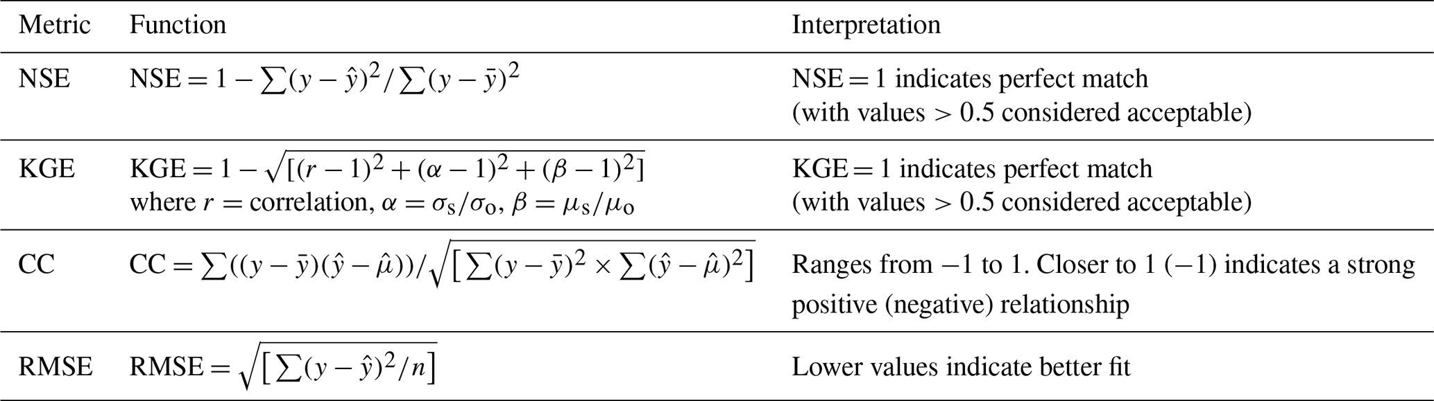
Model performance is assessed using several metrics (Table 1), including Correlation Coefficient (CC), Nash–Sutcliffe Efficiency (NSE), Kling–Gupta Efficiency (KGE), and Root Mean Square Error (RMSE). The best-performing LSTM–GNN configuration is compared against a baseline LSTM model that is independently trained from scratch as a standalone model. The baseline uses the same LSTM architecture and static feature integration as the LSTM component within the LSTM–GNN framework, but replaces the GNN routing module with a direct linear output layer for discharge prediction. Both models are trained independently using identical training data, loss functions, and optimization procedures, ensuring a fair comparison in which the only difference is the presence or absence of explicit spatial routing. We also investigate the effect of the GNN's message-passing range, which is determined by the number of graph layers (also referred to as hops). In this context, one hop allows a node to aggregate information directly from its immediate upstream neighbors, while two hops allow information to propagate from both immediate neighbors and their neighbors, and so on. To evaluate the impact of depth, we compare configurations ranging from 1-hop (one GNN layer) to 4-hop (four GNN layers) to identify the optimal propagation ranges.

Table 1 Hydrological performance metrics (y: Observed discharge, $\widehat{y}$: Estimated discharge, $\overline{y}$: Mean of observed discharge, $\widehat{\mathit{\mu }}$: Mean of estimated discharge, σ: Standard deviation of observed discharge, $\widehat{\mathit{\sigma }}$: Standard deviation of estimated discharge, n: Number of observations.

4 Results

4.1 Evaluation of LSTM–GNN models and Baseline LSTM

To assess the effectiveness of incorporating explicit spatial routing into deep learning models for streamflow prediction, we compared four LSTM–GNN architectures including LSTM-GCN, LSTM-GAT, LSTM-GraphSAGE, and LSTM-ChebNet against a baseline LSTM model. The evaluation was conducted across 530 gauging stations using four key metrics: NSE, KGE, CC, RMSE, and KGE components for the test period. Figure 3 presents boxplots of the metric distributions along with mean values for each model. Overall, all LSTM–GNN models significantly outperformed the baseline LSTM across all evaluation metrics (p<0.001, Friedman test). The LSTM–GAT achieved the highest mean NSE (0.61) and KGE (0.65), followed closely by GraphSAGE (NSE=0.60, KGE=0.60) and ChebNet (NSE=0.59, KGE=0.58). The GCN variant showed the lowest gains among the GNN-based models (mean NSE=0.48, KGE=0.50) but still surpassed the baseline LSTM (mean NSE=0.46, KGE=0.49). To further interpret the KGE improvements, we analysed its individual components including, correlation (CC), variability ratio (α), and bias ratio (β). The results show consistent improvements across all three components for the LSTM–GNN models relative to the baseline LSTM. The LSTM–GAT variant achieved the highest CC (0.84), α (0.87), and β (1.05), suggesting that graph-based spatial routing enhances temporal agreement, dynamic variability, and bias correction simultaneously. RMSE values decreased markedly for all GNN-based approaches, with LSTM–GAT showing the lowest median RMSE (13.77 m³ s⁻¹) compared to 21.24 m³ s⁻¹ for the baseline LSTM. The cumulative distribution functions (CDFs) of NSE (Fig. 4) further illustrate these improvements. The GNN–LSTM curves are consistently shifted to the right relative to the baseline, indicating a larger proportion of stations with higher NSE values, particularly for LSTM–GAT, GraphSAGE, and ChebNet. Scatter plots of normalized predicted versus observed discharge (Fig. 5), where flow values for each station are scaled to the [0,1] range, highlight the reduced bias and tighter clustering around the 1:1 line for LSTM-GNN models compared to the baseline. Among all models, LSTM–GAT predictions most closely align with the 1:1 line.

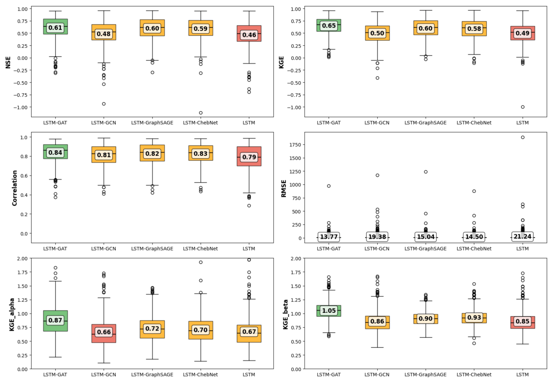
Figure 3 Boxplots comparing the baseline LSTM and four LSTM–GNN architectures (GAT, GCN, GraphSAGE, and ChebNet) across 530 stations using NSE, KGE, its components (α, β), correlation coefficient (CC), and RMSE (m³ s⁻¹) for 3_hop. Green boxes indicate the best-performing model for each metric, while red boxes denote the lowest-performing model. And others in yellow.

Figure 4 Cumulative distribution functions (CDFs) of Nash–Sutcliffe Efficiency (NSE) for the baseline LSTM and four LSTM–GNN models (GAT, GCN, GraphSAGE, ChebNet) across 530 subbasins.

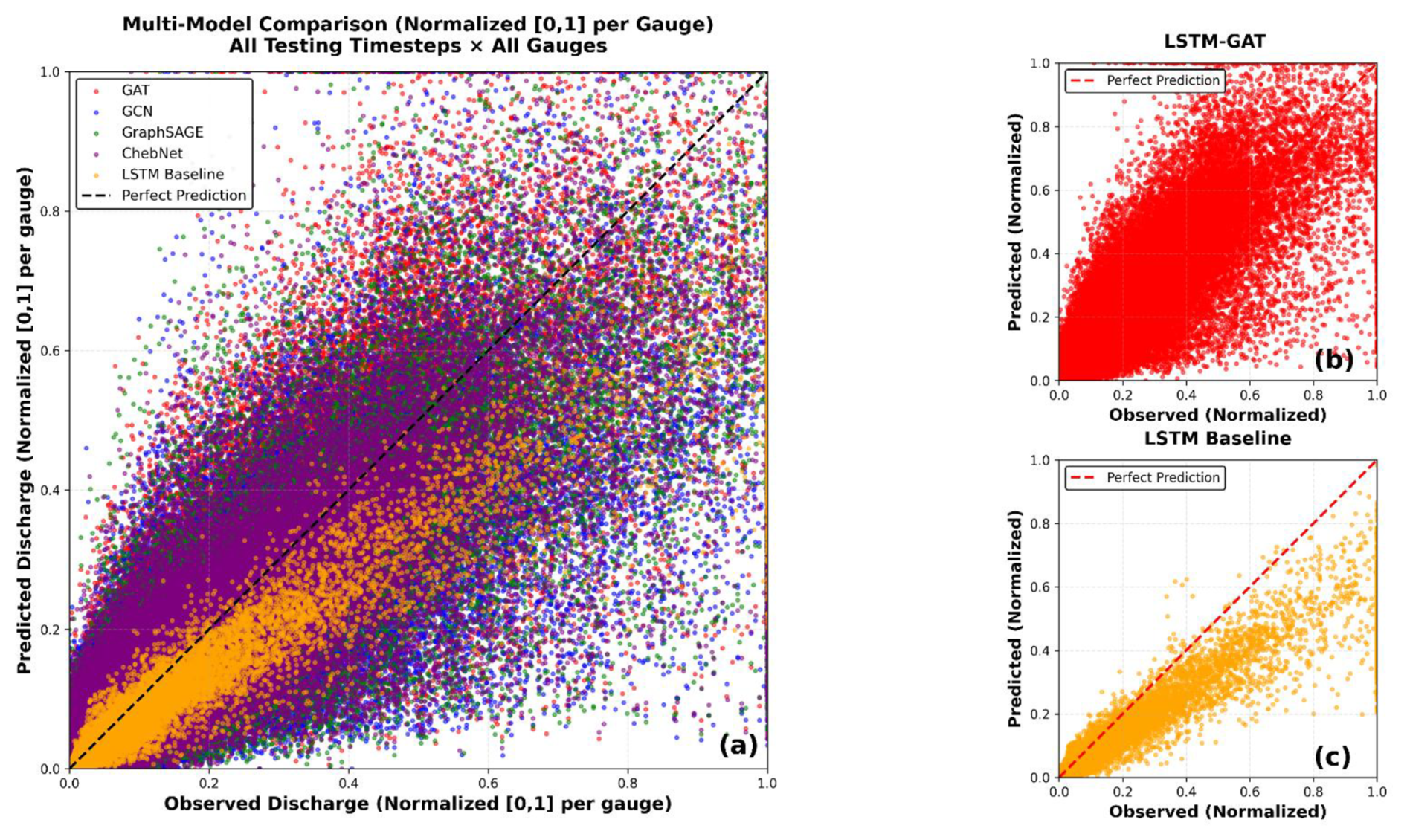
Figure 5 Scatter plots of normalized observed versus normalized predicted discharge for different models. (a) Multi-model comparison including LSTM baseline and LSTM–GNN variants (GAT, GCN, GraphSAGE, ChebNet). (b) LSTM–GAT and (c) baseline LSTM predictions.

4.2 Spatial and Network Drivers of LSTM-GNN Performance Improvements

To further investigate where the LSTM–GAT model, the best-performing GNN architectures, offers improvements over the baseline LSTM, we conducted a spatial comparison of performance metrics across all gauged stations. The difference in NSE values ($\mathrm{\Delta }\text{NSE}={\text{NSE}}_{\text{LSTM-GAT}}-{\text{NSE}}_{\text{LSTM}}$) was calculated for each of the 530 stations (Fig. 6). Positive differences, shown in blue, indicate locations where LSTM–GAT outperformed the baseline, while negative differences (red) denote stations where the baseline LSTM achieved higher NSE. River network thickness is scaled by upstream drainage area, and background colors show elevation from DEM. The analysis reveals that LSTM–GAT achieved higher NSE scores at 78 % of stations. Stations showing strong improvement (ΔNSE>0.25, blue) are predominantly located along major river reaches with large upstream drainage areas. Conversely, stations with negative changes (red dots) are concentrated in high-elevation headwaters.

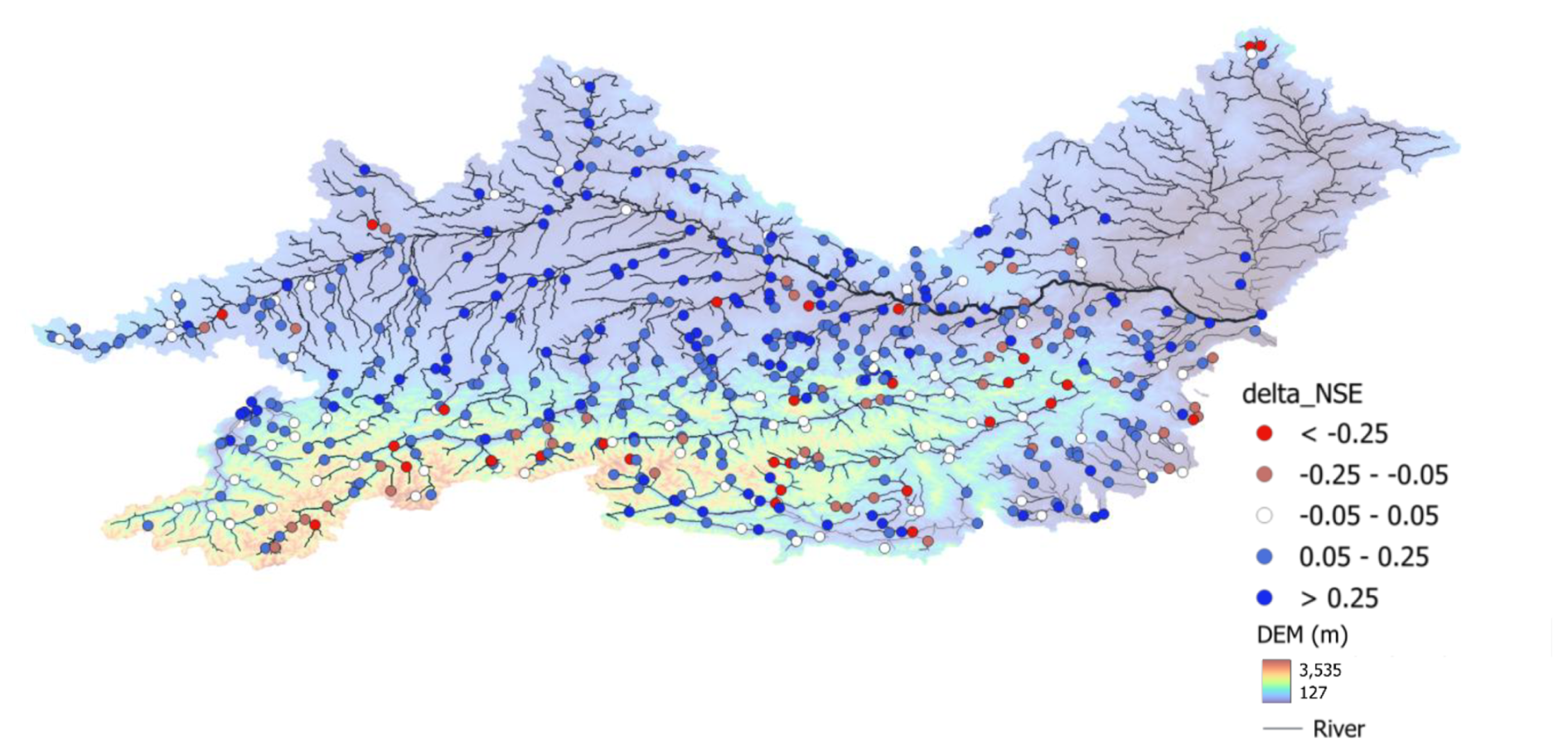
Figure 6 The spatial distribution of ΔNSE and ΔKGE across 530 stations. Blue markers indicate stations where LSTM–GAT outperformed the baseline LSTM (ΔNSE or ΔKGE>0.05), red where the baseline performed better ($\mathrm{\Delta }<-\mathrm{0.05}$), and white where the difference was negligible ($\left|\mathrm{\Delta }\right|\le \mathrm{0.05}$). Station colors represent five categories of ΔNSE: strong degradation ($<-\mathrm{0.25}$, red), moderate degradation (−0.25 to −0.05, light red), negligible change (−0.05 to 0.05, white), moderate improvement (0.05 to 0.25, light blue), and strong improvement (>0.25, blue). River network thickness is scaled by drainage area, with thicker lines indicating larger catchments.

To better understand the conditions under which the GNN-based routing provides the greatest benefit over the baseline LSTM, we examined the relationship between the change in NSE (ΔNSE) and a set of static physiographic and network-related attributes (Fig. 7). Spearman's rank correlation (ρ) was used to assess monotonic relationships, with significance levels indicated in each panel. Several network connectivity measures showed strong positive associations with ΔNSE. Total degree, which represents the number of direct upstream and downstream connections at a gauging station, was positively correlated (ρ=0.19, p<0.001), indicating that more connected nodes benefit more from GNN-based routing. Similarly, upstream contributing counts, the total number of upstream nodes that contribute flow to a given station, were positively associated with ΔNSE (ρ=0.23, p<0.001), suggesting that stations receiving flow from larger portions of the network see greater improvements. Betweenness centrality, which reflects how often a station lies along the main flow paths between other stations (i.e., major junctions or confluences within the river network), also showed a strong positive correlation (ρ=0.28, p<0.001). This suggests that hydrologically central nodes where multiple upstream tributaries converge benefit most from explicit routing, as GNN-based message passing effectively captures flow accumulation and redistribution at these critical junctions. Although betweenness centrality is partly related to the number of upstream nodes, it emphasizes the topological importance of stations that act as key connectors within the network rather than simply representing contributing area. Catchment size was likewise positively correlated with performance gains (ρ=0.25, p<0.001). Conversely, mean elevation ($\mathit{\rho }=-\mathrm{0.20}$, p<0.001) and mean slope ($\mathit{\rho }=-\mathrm{0.19}$, p<0.001) were negatively associated with ΔNSE, indicating smaller benefits for high-altitude or steep headwater sites.

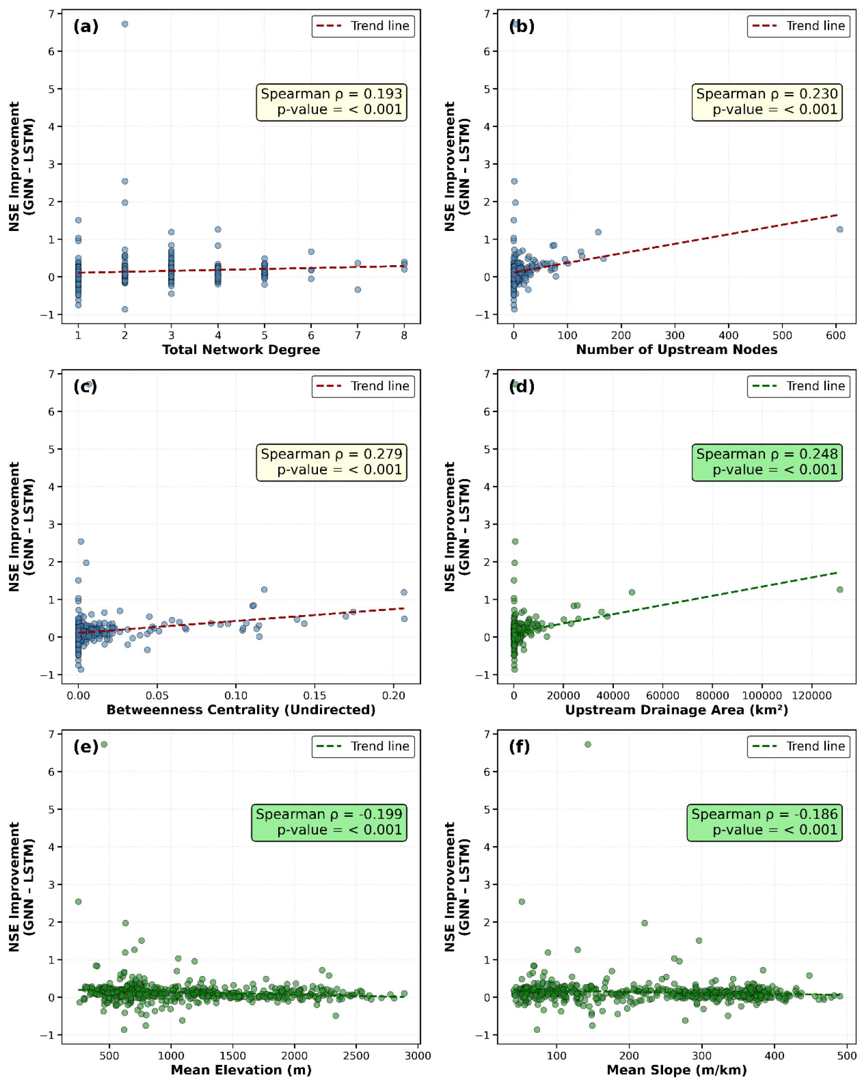
Figure 7 Relationship between performance improvement (ΔNSE) and (a) total network degree, (b) number of upstream nodes, (c) betweenness centrality (undirected), (d) upstream drainage area, (e) mean elevation, and (f) mean slope. Each panel shows scatter plots with Spearman's rank correlation coefficient (ρ) and significance levels. Positive ΔNSE values indicate stations where LSTM-GAT outperformed the baseline LSTM model.

To investigate the effect of message-passing range within the GNN, we evaluated the best-performing architecture (LSTM–GAT) using 1-hop, 2-hop, 3-hop, and 4-hop propagation settings. Figure 8 presents boxplots of NSE across the 530 stations, with mean values annotated for each configuration. Performance increased from a mean NSE of 0.57 with 1-hop to 0.60 with 2-hops. Extending the range to 3-hops yielded a slightly higher mean NSE (0.61), suggesting marginal additional benefit from including more distant upstream signals. However, increasing the propagation range to 4-hops reduced the mean NSE to 0.51, along with greater variability across stations. This decline is likely attributable to over-smoothing or gradient vanishing, where excessive message passing leads to homogenized node representations and loss of local detail.

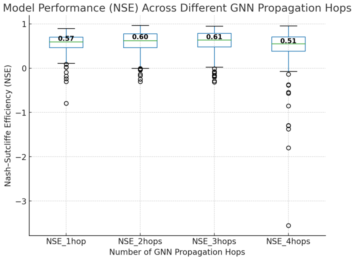
Figure 8 Boxplots showing the distribution of NSE values across 530 stations for different hop ranges in the LSTM-GAT model.

5 Discussion

This study set out with the hypothesis that integrating a GNN-based routing component into a R–R model would yield improved prediction accuracy over a standalone LSTM model. The results strongly support this hypothesis. Across all performance metrics including NSE, KGE, CC, and RMSE the LSTM–GNN model significantly outperformed the baseline LSTM, which lacked explicit routing. In other words, explicitly modeling runoff routing via a GNN led to more accurate streamflow predictions. Our findings are consistent with Cortés-Salazar et al. (2023) demonstrated that including routing in a physical model significantly improved performance (KGE increased from 0.64 without routing to 0.81 with routing). Similarly, Kraft et al. (2025) showed that incorporating routing into lumped LSTM baselines across Switzerland yielded substantial performance gains (KGE improvements of 24 %–62 %). The analysis further revealed that the benefits of GNN-based routing vary across the river network, with the largest performance improvements occurring at stations with larger upstream contributing areas and stronger network connectivity. To illustrate this, we analyzed a cluster of three stations within a connected sub-network of the Isel River system: Matreier Tauernhaus (Station 532) on the Tauernbach River, Waier (Station 530) on the Isel River, and Bruehl (Station 533) also on the Isel River (Fig. 9), with a combined contributing catchment area of approximately 518.4 km². These stations are arranged along a flow path from upstream to downstream, with Station 530 representing a major junction that aggregates flow from multiple tributaries. At the upstream site (Station 532), where flow is primarily driven by local precipitation and routing effects are limited, the performance difference between LSTM and LSTM–GAT was small, and the baseline model slightly outperformed the GNN-enhanced model. However, at the downstream junctions (Stations 530 and 533), the LSTM–GNN achieved much higher NSE values (0.92 vs. 0.82 at Station 530; 0.90 vs. 0.76 at Station 533). Hydrograph comparisons confirm that the GNN-based model reproduced peaks more accurately, improving both magnitude and timing, whereas the baseline LSTM systematically underestimated high-flow events. These results demonstrate that GNN-based routing is particularly effective in downstream locations where hydrological signals accumulate from multiple upstream areas. Importantly, performance gains were also observed at gauges with only two or three upstream connections, suggesting that even relatively sparse networks can benefit from explicit routing.

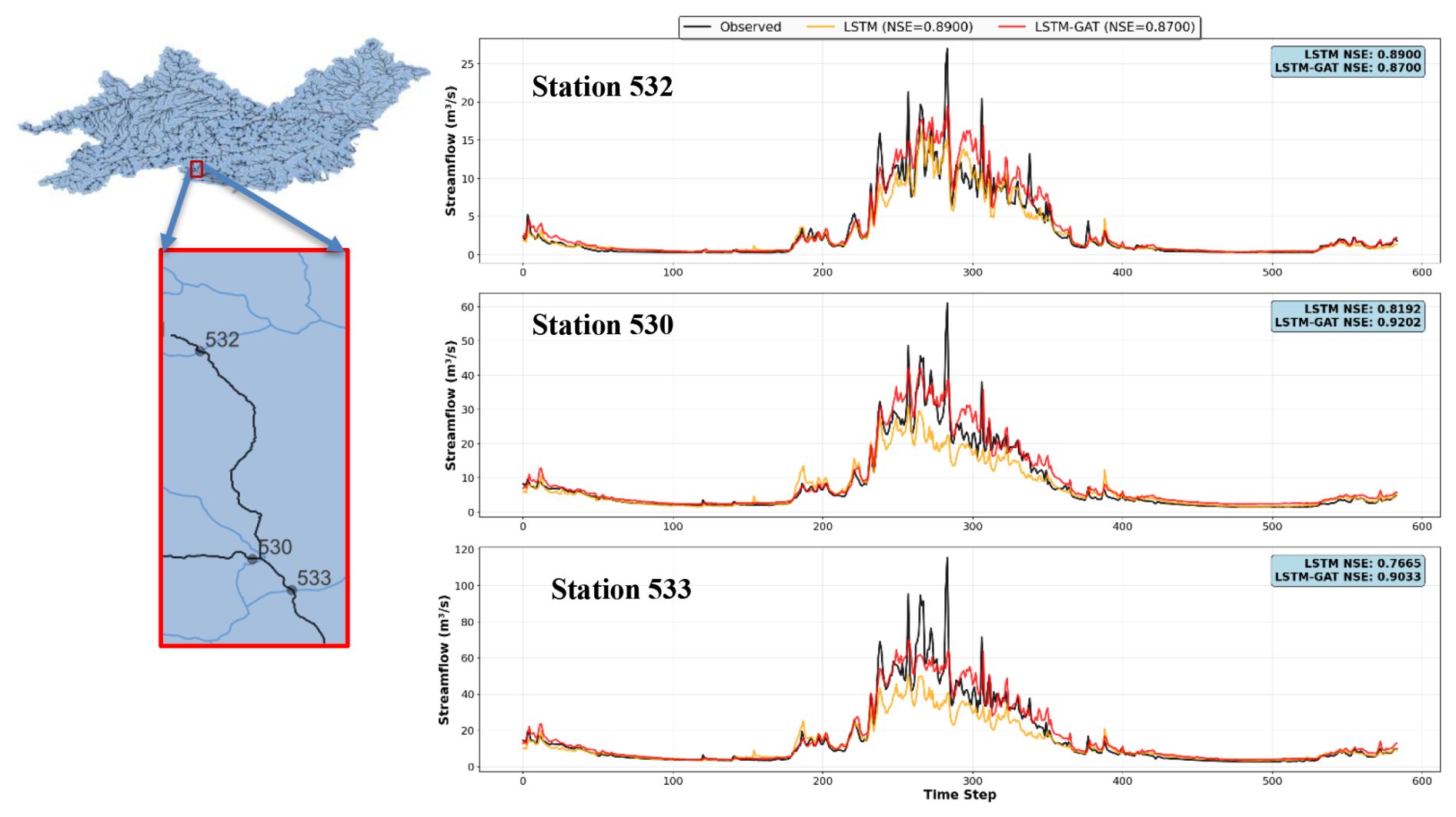
Figure 9 Hydrograph comparisons between LSTM and LSTM–GAT models at Matreier Tauernhaus (Station 532), Waier (Station 530), and Bruehl (Station 533) on the Isel River system.

At the basin scale, the largest improvements occurred in large, lowland subbasins, and catchment size was positively correlated with performance gains. This indicates that larger basins, where extensive flow accumulation and routing dominate, particularly benefit from GNN-based modeling. This addresses a well-known limitation of LSTM models in large river basins, where their lack of explicit routing can hinder performance. Conversely, in high-slope headwater basins and at the most upstream gauges, the baseline LSTM often performed equally well or better, reflecting the fact that hydrological response in these locations is primarily driven by local precipitation and rapid runoff processes, with minimal routing influence.

Among the different LSTM–GNN configurations tested, the model using a GAT achieved the best performance. It delivered the highest NSE, KGE, and correlation values, outperforming GCN, GraphSAGE, and ChebNet. The improved results of the GAT-based model likely stem from its ability to assign adaptive weights to different upstream neighbors during message passing. In hydrological terms, this means the model can learn which tributaries or upstream catchments exert a stronger influence on downstream flow, rather than treating all upstream nodes equally. This adaptivity is particularly important in heterogeneous networks such as the Danube Basin, where tributaries differ greatly in size, slope, and hydrological response. Our results align with Deng et al. (2024), who also reported that attention-based graph architectures outperform others in hydrological prediction tasks. Together, these findings highlight that capturing heterogeneous upstream contributions is essential for accurate routing, making the LSTM–GAT framework the most effective among the tested models.

To provide a practical perspective on model efficiency, we also recorded the average training time per epoch for each architecture. The baseline LSTM required approximately 56 s per epoch, whereas the LSTM–GNN models ranged from 68 s for LSTM–GAT and 69 s for LSTM–GCN to 73 s for LSTM–GraphSAGE and 79 s for LSTM–ChebNet. As expected, the LSTM–GAT required roughly 20 % longer training time than the baseline, reflecting the additional computational cost of graph-based message passing. However, this increase remains modest relative to the performance gains achieved. Moreover, inference time, relevant for real-time or operational applications, was comparable across all models, indicating that the GNN-based extensions do not introduce substantial computational overhead during prediction.

6 Conclusion

This study introduced a novel LSTM–GNN framework for R–R modeling that explicitly integrates runoff generation and runoff routing within a unified deep learning architecture. By leveraging LSTMs to capture local temporal dynamics and GNNs to model spatial dependencies across the river network, the proposed approach addresses a major limitation of existing data-driven hydrological models: the absence of physically consistent flow routing. Applied to the Upper Danube River Basin, our model demonstrated significant improvements over a baseline LSTM model that neglects explicit routing. Among the tested GNN variants, the GAT emerged as the most effective, achieving the highest mean NSE (0.61), KGE (0.65), and CC (0.84), while reducing RMSE by approximately 35 % compared to the baseline. These enhancements were particularly pronounced in downstream stations with high network connectivity and large contributing areas, where routing effects dominate hydrological responses, underscoring the value of adaptive message passing in capturing heterogeneous upstream influences.

The findings affirm our hypothesis that integrating GNN-based routing enhances predictive accuracy, especially in complex, large-scale basins like the Danube, where flow accumulation and delays play a critical role. This approach not only improves streamflow forecasting but also advances the physical interpretability of deep learning models by aligning their structure with real-world hydrological processes. While we did not specifically test predictions in completely ungauged basins, the model's design, relying solely on meteorological and static catchment data without the need for past flow observations, enables such applications in principle. Future work should evaluate the model's performance in ungauged basins to validate its generalizability and assess its potential for water resource management, flood risk assessment, and climate change adaptation in data-scarce regions.

Despite these advancements, opportunities for further refinement remain. Future work should explore evaluating the model across diverse global basins to validate its generalizability. Future work could also investigate transfer-learning strategies such as regional pre-training followed by limited subbasin fine-tuning, which may improve performance in hydrological outliers and enhance model transferability to unseen basins. Incorporating dynamic edges in the GNN model using variables like soil moisture could be another approach to test. In addition, hybrid comparisons that combine graph-based routing with simple process-based runoff or routing schemes could help further clarify the complementary roles of physical and data-driven approaches. Ultimately, this study highlights the transformative potential of graph neural networks in hydrological modeling, paving the way for more spatially aware and accurate predictions in an era of increasing environmental challenges.