Evaluating E-OBS forcing data for large-sample hydrology using model performance diagnostics

For large-sample hydrological studies over large spatial domains, large-scale meteorological forcing data are often desired. For Europe, the EStreams dataset and catalogue satisfies this demand. In EStreams, the meteorological time series are obtained from the Ensemble Observation (E-OBS) product which is available for all of Europe. Due to the large spatial extent of this dataset, limitations and regional variations of data quality have to be expected when the dataset is compared to smaller-scale datasets, e.g., at national level. In this study, we compare the meteorological time series included for 2682 catchments in EStreams to eight smaller datasets (mostly CAMELS datasets). We assess how the different meteorological data impact the performance of a bucket-type hydrological model. For most catchments, the precipitation amounts derived from E-OBS are lower than the ones from the CAMELS data, while the temperature and the potential evapotranspiration values are higher. Model performances tend to be lower when the E-OBS data are used than when the CAMELS datasets are used for calibration. Exceptions arise when the station density in the E-OBS data is high. This study provides the first assessment of the E-OBS data at a continental scale for hydrological applications and shows that, despite some limitations, the dataset offers a reasonable basis for large-sample hydrological modelling across Europe.

1 Introduction

Driven by their enormous value for hydrological modelling studies, large-sample hydrology (LSH) datasets have developed at a rapid pace in the past decades, and the development continues to gain momentum: Since 2017, more than a dozen “CAMELS” datasets were released or are being developed (Addor et al., 2017; Alvarez-Garreton et al., 2018; Bushra et al., 2025; Chagas et al., 2020; Coxon et al., 2020a; Delaigue et al., 2025a; Fowler et al., 2021; Höge et al., 2023; Jimenez et al., 2025; Liu et al., 2025; Loritz et al., 2024; Mangukiya et al., 2025; Nijzink et al., 2025; Teutschbein, 2024a). Other animals entered the LSH stage as well: Llamas (Helgason and Nijssen, 2024; Klingler et al., 2021), a goat (cabra in Portuguese; Almagro et al., 2021), and a bull (Senent-Aparicio et al., 2024b).

In the past years, efforts also went into the creation of more overarching products, i.e., datasets covering not only one country or region. The Caravan dataset (Kratzert et al., 2023) combined the streamflow data from thousands of catchments in already published open source LSH datasets with meteorological time series and catchment attributes from the global ERA5-Land reanalysis (Muñoz-Sabater et al., 2021). Caravan is growing further and has become a quasi-global dataset (Färber et al., 2024). For Europe, a dynamic dataset and a catalogue that provides detailed guidance for retrieving streamflow data from national providers were introduced in EStreams (https://www.estreams.eawag.ch, last access: 22 December 2025) by do Nascimento et al. (2024a).

Although these collections of large-sample datasets are valuable resources, the combination of catchments distributed across different regions and especially across different countries in one dataset almost always goes hand in hand with difficulties in providing high-quality streamflow and forcing data. This is due to the lower availability of high-quality data for larger spatial extents, while smaller datasets typically benefit from more thorough quality control. Furthermore, data processing choices (e.g., gap filling, interpolation) are more often required at large scales and might introduce added uncertainty in the outcomes (McMillan et al., 2018).

In an earlier study, Clerc-Schwarzenbach et al. (2024) showed that the globally available meteorological data obtained from ERA5-Land (Muñoz-Sabater et al., 2021) in the Caravan dataset (Kratzert et al., 2023) led to a consistently lower hydrological model performance for catchments in the US, Brazil, and Great Britain, compared to when the meteorological forcing data from the corresponding CAMELS datasets (Addor et al., 2017; Chagas et al., 2020; Coxon et al., 2020a) were used. This demonstrates the importance of promoting awareness of potential data quality losses when it comes to large-scale meteorological datasets.

Similar to the ERA5-Land data in Caravan, the meteorological data were also obtained from a large-scale dataset in EStreams (do Nascimento et al., 2024a). For EStreams, the data were obtained from the European Ensemble Observation (E-OBS) product (Cornes et al., 2018). After the publication of EStreams, questions on the quality of the meteorological forcing data from E-OBS arose in the LSH community. Recent studies have evaluated the accuracy of the E-OBS precipitation product against reference datasets and meteorological stations in some parts of Europe, including Greece (Mavromatis and Voulanas, 2021), the central Alps, eastern Europe and Scandinavia (Bandhauer et al., 2022). These evaluations indicated that the quality of the E-OBS precipitation data, when compared to data from high-resolution datasets focusing on a smaller area, is higher in regions with a high density of E-OBS stations, such as in central Europe, while the reanalysis product ERA5 (Hersbach et al., 2020) partly outperformed E-OBS in regions with a sparse station network (Bandhauer et al., 2022). Yet, evaluations of the E-OBS data over a larger extent, and specifically for hydrological modelling, remain unexplored.

To be able to inform the users of EStreams (and of the E-OBS data in general) about the effects of the harmonized meteorological data on hydrological applications, a comparison to the meteorological data contained in different national and regional datasets (i.e., CAMELS datasets and similar products) is required.

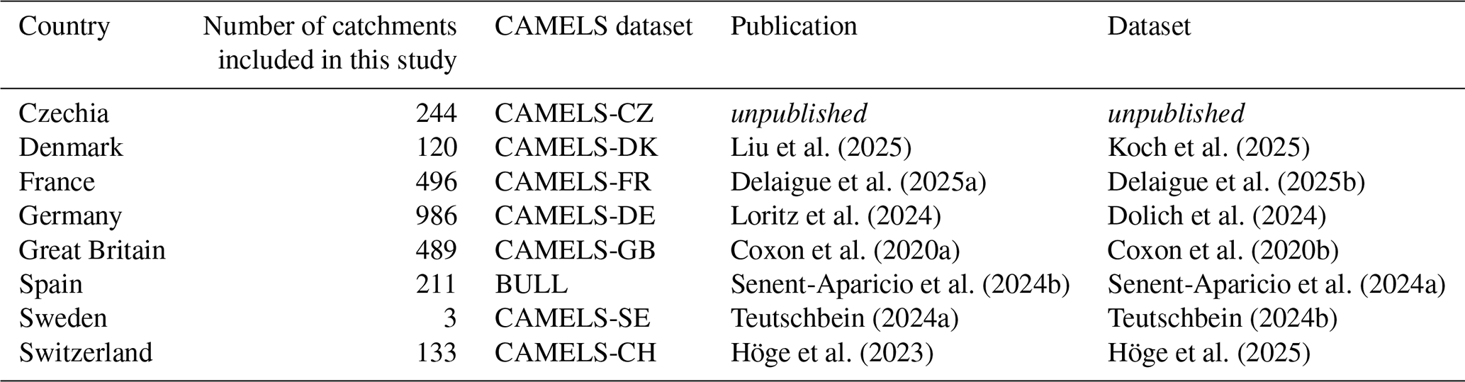
For this study, we used 2682 catchments from eight European countries and assessed the hydrological efficacy of the meteorological data provided in EStreams (obtained from E-OBS). We did so by comparing the meteorological forcing data from E-OBS to the analogous data contained for the same catchments in national or regional datasets, namely in CAMELS-DK (Liu et al., 2025) for Denmark, CAMELS-FR (Delaigue et al., 2025a) for France, CAMELS-DE (Loritz et al., 2024) for Germany, CAMELS-GB (Coxon et al., 2020a) for Great Britain, the BULL Database (Senent-Aparicio et al., 2024b) for Spain, CAMELS-SE (Teutschbein, 2024a) for Sweden, and CAMELS-CH (Höge et al., 2023) for Switzerland. In addition, we also included catchments from Czechia, with data from the not yet published CAMELS-CZ dataset (Jenicek et al., 2024). The meteorological data in the smaller datasets stem from sources that were created specifically for the respective country.

The methodology used in this work is based on the one presented by Clerc-Schwarzenbach et al. (2024). Following their approach, we did not only compare the meteorological data itself, but also the model performances that were achieved with the different meteorological forcings (but same streamflow data) when calibrating the bucket-type HBV (Hydrologiska Byråns Vattenbalansavdelning) model (Bergström, 1992, 1995; Seibert and Vis, 2012). This allowed us to assess the overall hydrological efficacy of the forcing data.

The reasoning behind this approach is that hydrological models are not only useful for simulating streamflow but can also be used as diagnostic tools to evaluate the efficacy of the input data (Beck et al., 2017; Tarek et al., 2020). The rationale is that, although hydrological models are inherently imperfect representations of reality, systematic differences in their performance when driven by different datasets are unlikely to be random. As noted by Linsley (1982, p. 13), “if the data are too poor for the use of a good simulation model, they are also inadequate for any other model”. Building on this idea, our study uses the HBV model as a means to assess the hydrological reliability of different meteorological forcing data across Europe. Therefore, we assume that if a model consistently performs better with one dataset than with the other, this difference likely reflects a closer alignment of the corresponding meteorological data with the actual processes in the catchment.

2 Data and Methods

2.1 Subset of catchments

We conducted this study for 2682 catchments that are available in the EStreams dataset and catalogue and in one of the following datasets: CAMELS-CZ, CAMELS-DK, CAMELS-FR, CAMELS-DE, CAMELS-GB, BULL, CAMELS-SE, CAMELS-CH, for simplicity's sake referred to as the “CAMELS datasets” throughout the remainder of the paper (Table 1). These catchments fulfilled the following cascade of criteria (with the number of catchments still included after each step in brackets, see also Fig. S1 in the Supplement):

• Located in a country with access to a CAMELS dataset at the time of data preparation, i.e., Austria, Czechia, Denmark, France, Germany, Great Britain, Iceland, Spain, Sweden, or Switzerland [12 019]

• High-quality catchment delineation in EStreams, as described by do Nascimento et al. (2024a) [10 434]

• Catchment area (obtained from EStreams) below 2000 km² [9115]

• No redundancy among the EStreams catchments (the catchment with the longer streamflow time series was kept) [8909]

• Availability of at least 90 % of the potential evapotranspiration (E_pot) data between October 1990 and September 2015 [8846]

• Availability of the catchment in one of the CAMELS datasets [3557]

• CAMELS forcing data coming from a smaller-scale dataset (catchments from LamaH-CE (Austria) excluded as meteorological forcings are from ERA5-Land) [3097]

• Availability of at least 90 % of the streamflow data (in the CAMELS dataset) between October 1995 and September 2015 [3097]

• Maximum five lakes upstream (obtained from EStreams) [2841]

• Normalized upstream capacity of reservoirs, calculated using Eq. (9) from Salwey et al. (2023), and derived from the EStreams dataset, smaller or equal than 0.2 [2741]

• Runoff ratio (based on the precipitation data from the CAMELS dataset) between October 1995 and September 2015 below 1.1 [2741]

• Runoff ratio (based on the precipitation data in EStreams) between October 1995 and September 2015 below 1.1 [2682]

We excluded catchments with an area of more than 2000 km² as a bucket-type hydrological model is not the most suitable choice for larger catchments.

Table 1 Overview of catchments and data sources used in this study.

Unlike the other national datasets, the LamaH-CE dataset for Austria uses ERA5-Land as its meteorological forcing. As the comparison of E-OBS data to globally available data is a different question than the comparison to smaller-scale (national) products, we excluded the Austrian dataset from the analyses. Moreover, a previous study already highlighted several limitations of ERA5-Land as forcing for hydrological models (Clerc-Schwarzenbach et al., 2024).

To minimize the inclusion of catchments potentially affected by human regulation (e.g., reservoirs or diversions), we applied two attribute-based criteria. The maximal number of lakes was chosen arbitrarily, with the goal of excluding highly regulated catchments. The second criterion, the normalized upstream capacity, was calculated following Salwey et al. (2023), and a threshold of 0.2 was adopted based on their findings. While these filters may exclude some basins that are only weakly influenced by regulation, we preferred a conservative approach. Moreover, we selected these two criteria because the relevant information (number of lakes and upstream capacity) is consistently available across Europe in the EStreams dataset, allowing for a uniform filtering procedure even where metadata on human influence are not provided in the national CAMELS datasets.

Following a similar reasoning, we excluded catchments with runoff ratios greater than 1.1, as natural streamflow rarely exceeds precipitation by such large margins in unregulated basins. Such cases likely reflect data inconsistencies or strong anthropogenic influence (e.g., diversions or regulation).

Finally, to make sure that the streamflow data (obtained from the CAMELS datasets) were reasonable, we checked that the average streamflow was not unrealistically high (i.e., not exceeding 10 mm d⁻¹ as this may indicate issues with the data) which was the case for all 2682 catchments.

2.2 Meteorological data

For the data comparison and the modelling experiments, we investigated and used daily precipitation, E_pot, and temperature data from the EStreams dataset and from the different CAMELS datasets (Table 1). We used the latest released version of EStreams (version 1.4), for which precipitation and temperature data were obtained from the E-OBS ensemble mean product with a spatial resolution of 0.1° in both latitude and longitude (do Nascimento et al., 2025). E-OBS provides a pan-European observational dataset of surface climate variables that is derived by statistical interpolation of in-situ measurements, collected from national data providers (Cornes et al., 2018). E_pot time series in EStreams were calculated with the Hargreaves formula (Hargreaves and Samani, 1982), using the E-OBS temperature data and catchment elevation as input. Note that there is also a version of E-OBS at a resolution of 0.25° available and originally represented in EStreams. Users should be aware that different resolutions of a forcing dataset can lead to slightly different performances. Similarly, there are different E_pot products available from E-OBS as derived indices, but here, we used the E_pot product provided in EStreams. The CAMELS meteorological data are usually based on in-situ observations. When more than one option was available, we chose the data with the highest spatial and (original) temporal resolution to represent the CAMELS data for this study (Table 2). While E-OBS was developed specifically for Europe, one can still expect a lower data quality than for datasets created for a smaller region (e.g., national datasets) due to the lower spatial resolution and interpolation choices used to achieve the larger spatial extent of the dataset.

Table 2 Overview of the data sources for the meteorological data (precipitation P, temperature T, and potential evapotranspiration E_pot) for the different CAMELS datasets in this study.

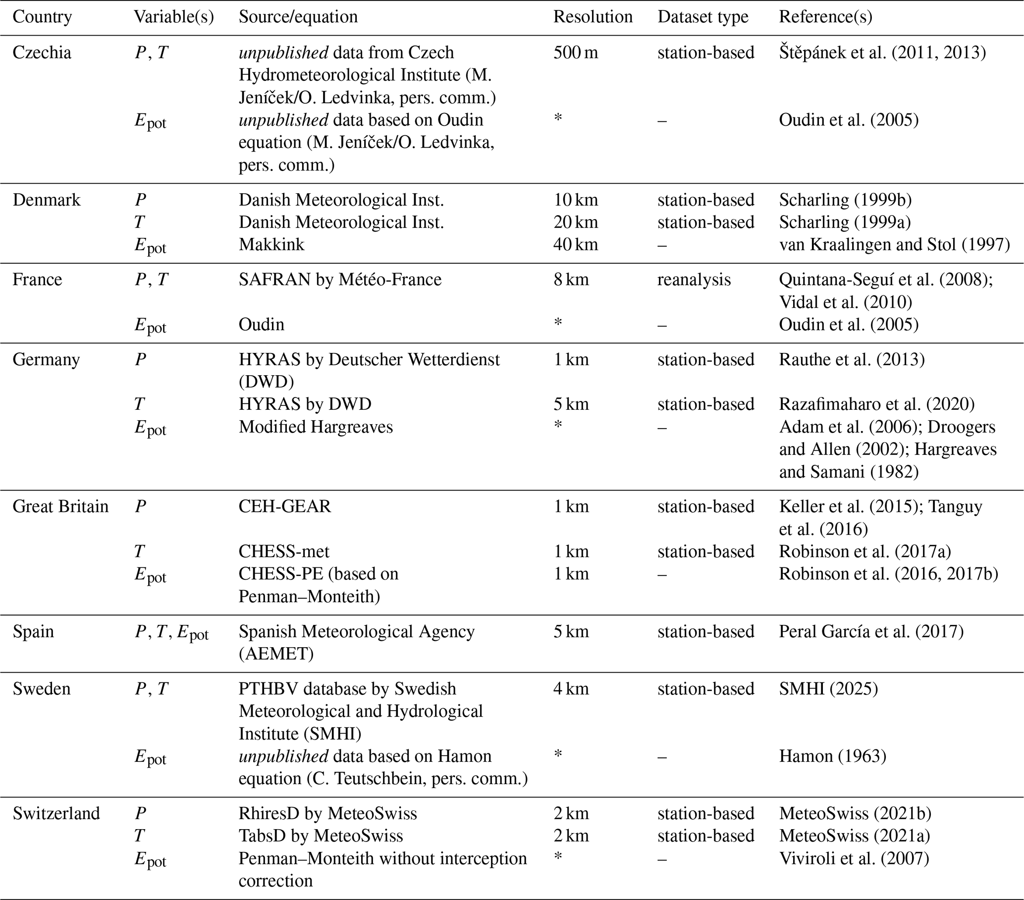
* calculation for each catchment based on its meteorological data

Note that the shapefiles that were used in EStreams and in CAMELS to calculate the areal averages for the meteorological forcings potentially differed. In addition to the different data sources, this can affect the forcing data.

2.3 Calculations of the differences in the CAMELS and E-OBS data

We compared the precipitation, E_pot, and temperature data from EStreams (i.e., the E-OBS data) to the corresponding data from the different CAMELS datasets (Table 2) for the twenty years between October 1995 and September 2015 to get an overview of the differences in the data. For precipitation and E_pot, we determined the relative difference in the mean annual sums. For temperature, we determined the mean absolute difference for the daily data. When comparing the two datasets, we used the E-OBS data obtained from EStreams as minuend and the analogous data obtained from the CAMELS datasets as subtrahend, i.e., positive differences indicate higher values in the E-OBS data, while negative differences indicate lower values in the E-OBS data than the CAMELS data. To calculate relative differences (for precipitation and E_pot), we divided by the mean annual sum determined from the CAMELS dataset. Thus, for example, a value of −20 % indicates that the mean annual sum obtained from E-OBS is 80 % of the mean annual sum obtained from the CAMELS dataset, and a value of 40 % indicates that the mean annual sum obtained from E-OBS equals 140 % of the mean annual sum obtained from the CAMELS dataset.

2.4 Modelling experiments

Following the methodology of Clerc-Schwarzenbach et al. (2024), we defined different combinations of forcing data (“scenarios”) to calibrate the hydrological model (Table 3). This allowed us to determine how the forcing data and their individual variables impacted hydrological model performance. Since EStreams does not provide daily streamflow data, but where to find them, we used the observed streamflow data contained in the CAMELS datasets for all modelling experiments. Thus, we made sure that the hydrological model performance was not affected by different streamflow data.

Table 3 Combinations of forcing data (“scenarios”) for the modelling experiments.

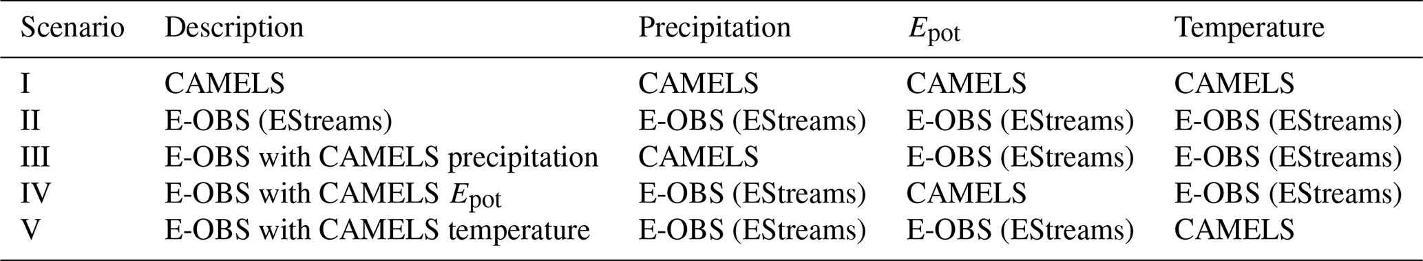
In the first two scenarios, we used the CAMELS forcing data (scenario I) or the E-OBS data obtained from EStreams (scenario II). To isolate the impact of the forcing variables, we additionally defined three mixed scenarios. Scenario III used precipitation from CAMELS and E_pot and temperature from E-OBS. Similarly, scenario IV evaluated the effect of using only E_pot from CAMELS, and consequently if using different E_pot formulations would change our results, while scenario V assessed the effect of using only temperature from CAMELS. Note that due to the dependency of the E-OBS E_pot data on the E-OBS temperature data, model calibration was influenced by the E-OBS temperature data even when replacing the temperature data from E-OBS with those from CAMELS (scenario V).

Analogously to Clerc-Schwarzenbach et al. (2024), we calibrated the HBV model (Bergström, 1992, 1995) in the version HBV-light (Seibert and Vis, 2012) with a genetic algorithm (Seibert, 2000). Each catchment was divided into elevation zones of 200 m elevation difference, whereby an elevation zone had to account for at least 5 % of the catchment area. For the determination of the elevation zones, we used the shapefiles provided by EStreams, and the Copernicus DEM at a resolution of 30 m (European Space Agency and Airbus, 2022).

We used the five years from October 1990 to September 1995 as the warming-up period for the model, and the twenty years from October 1995 to September 2015 as the simulation period for which we optimized daily streamflow simulation in terms of the Kling–Gupta efficiency KGE (Gupta et al., 2009). One calibration consisted of a total of 3500 model runs. We conducted each calibration ten times to account for equifinality. We used equal weights on the ten simulated hydrographs to calculate an ensemble mean hydrograph. We determined the model performance (using again the KGE as well as the PBIAS, i.e., the percent bias of the simulated streamflow compared to the observed one) for each catchment and each scenario by comparing this ensemble mean hydrograph to the observed hydrograph.

2.5 Statistical tests

We used the Spearman rank correlation coefficient (r) and corresponding p-values to assess the relationships between the model performance differences in terms of the KGE and different catchment attributes. We used the locally-weighted polynomial regression (lowess; Cleveland, 1979) to visually represent the relationships. In addition, we used the Wilcoxon signed-rank test (Wilcoxon, 1945) on paired median KGE values to evaluate whether the differences in model performance between the scenarios were statistically significant.

3 Results

3.1 Comparison of the meteorological data

The mean annual precipitation sums in the E-OBS data were lower than the mean annual precipitation sums in the CAMELS data for 2362 catchments (88 %). For 758 catchments (28 %), the deviation of the mean annual precipitation sums in E-OBS from the ones in CAMELS exceeded −10 %. Conversely, there were only 33 catchments (1 %) for which the mean annual precipitation sums in E-OBS were overestimated by +10 % or more from the ones in CAMELS. Differences between the two data sources were largest for the catchments in Spain and smallest for the catchments in Germany (Fig. 1).

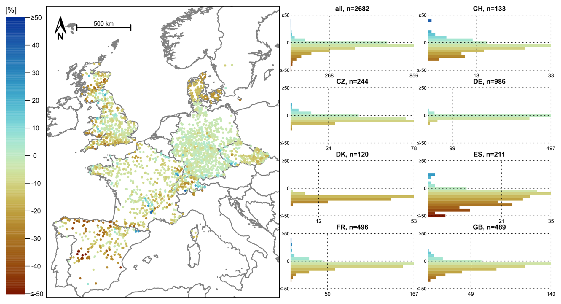
Figure 1 Relative difference in the mean annual precipitation (for a 20 yr period: 1995–2015) between the E-OBS data obtained from EStreams and the different CAMELS datasets. Negative values and brown colours indicate less precipitation in E-OBS than in CAMELS, positive values and blue colours more precipitation in E-OBS. On the map, the catchments with the largest deviations were plotted last to increase their visibility. Note that there is no separate histogram for the three catchments in Sweden and that the number of catchments per histogram differs. This is illustrated by the vertical lines indicating 10 % (rounded) of the number of catchments per histogram. The colour scale was cut at ±50 %. The scale bar refers to the map center. The base map was obtained from Natural Earth (naturalearthdata.com). The colour palette used in this and all other maps are scientific colour palettes from Crameri (2023).

The opposite was found for the annual sums of E_pot: For 2508 catchments (94 %), the mean annual E_pot calculated from the E-OBS data was higher than for the CAMELS data. For 1353 catchments (50 %), the deviation of the E-OBS E_pot sums from the CAMELS E_pot sums were at least 10 %. Clearly lower E_pot sums derived from E-OBS than from CAMELS could only be observed for catchments in Sweden, on the Danish islands, in southern Switzerland, and for some catchments in northern Spain (Fig. 2). As different equations or data sources were used in the different CAMELS datasets (see Table 2) to obtain the E_pot data, the order of magnitude of the deviations changed abruptly along the national borders in some cases (e.g., along the border between Czechia and Germany). It is noteworthy that for E_pot, there tend to be small differences between the two datasets for Spain (while this was not the case for precipitation).

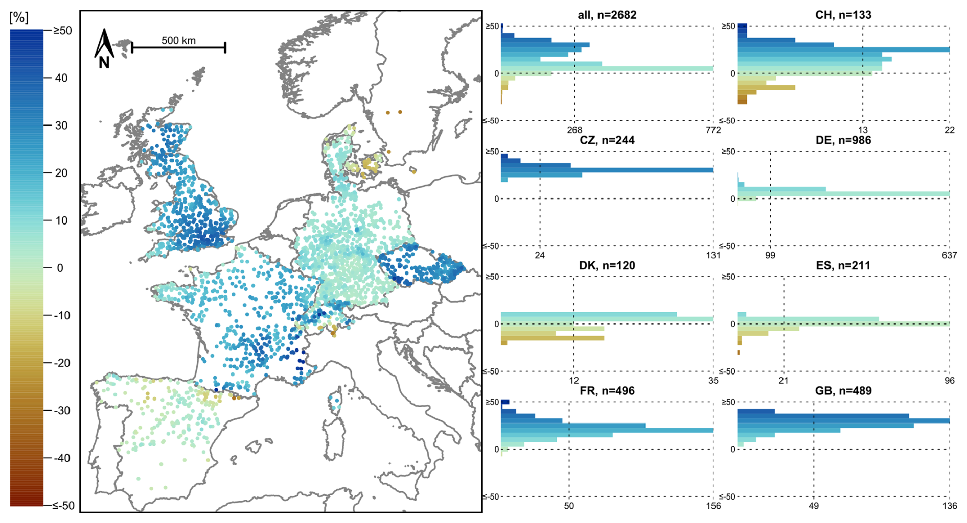
Figure 2 Relative difference in the mean annual E_pot (for a 20 yr period: 1995–2015) obtained from EStreams and calculated from the E-OBS data compared to the mean annual E_pot calculated from the different CAMELS datasets. Negative values and brown colours indicate a lower E_pot in E-OBS than in the CAMELS datasets, positive values and blue colours a higher E_pot in E-OBS. On the map, the catchments with the largest deviations were plotted last to increase their visibility.

Due to the differences in the precipitation and the E_pot data, the aridity indices ($E_{\text{pot}}/P$) calculated from the two data sources differed, although they were still highly correlated (Pearson's correlation coefficient of 0.94) (Fig. 3). Given the lower precipitation and higher E_pot sums for most catchments, the aridity indices were generally higher when the E-OBS data obtained from EStreams were used than when the CAMELS data were used. This did not apply for Sweden, as the E_pot sums based on E-OBS were lower than the ones from CAMELS for this country. The two calculated aridity indices aligned best for Germany and worst for Spain, Great Britain, and Czechia. Spatially, the aridity indices derived from both datasets followed the expected pattern, with more arid catchments in southern Europe and north-eastern Germany and more humid catchments in the other regions (see Fig. A1 for the CAMELS data and Fig. A2 for the E-OBS data).

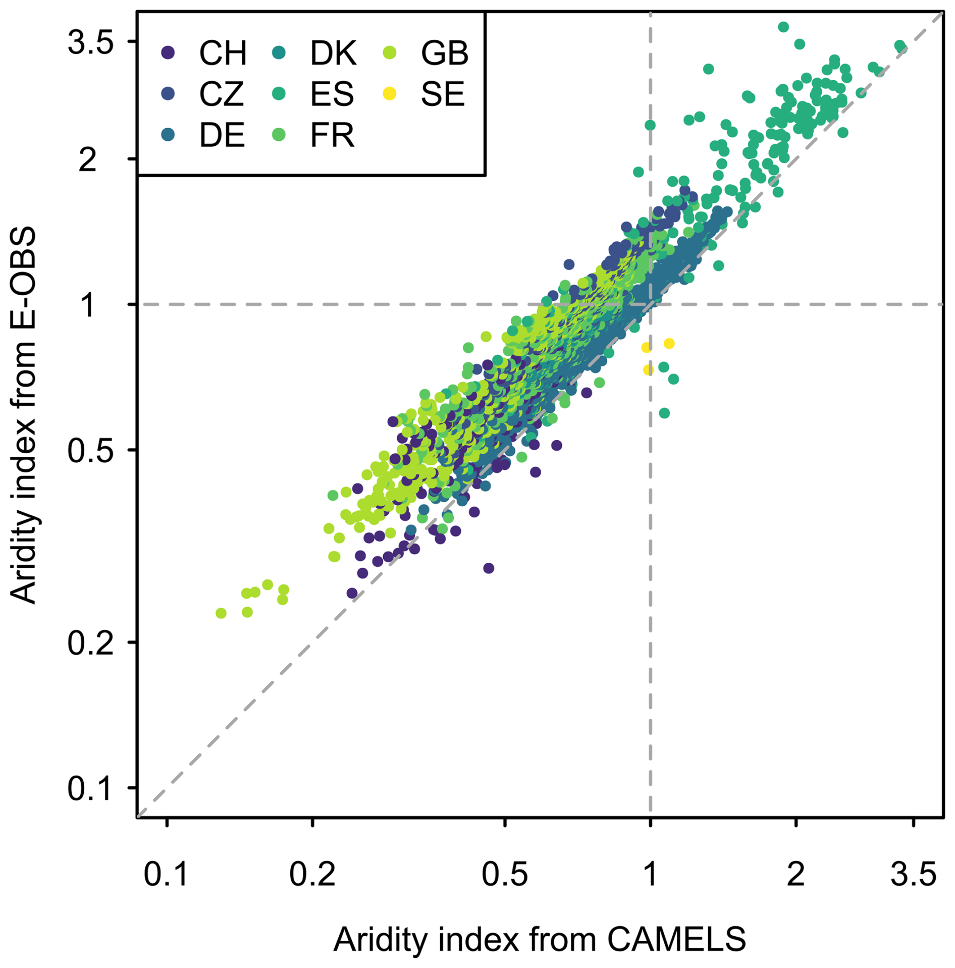
Figure 3 Comparison of the aridity indices ($E_{\text{pot}}/P$) based on the CAMELS and the E-OBS data (for a 20 yr period: 1995–2015), colour-coded by country. Note the logarithmic axes.

Comparison of the temperature data in the two datasets revealed that the average temperature in E-OBS was higher (median difference: 0.3 °C) for most catchments than the average temperature in CAMELS (see Fig. S2 in the Supplement). There were 636 catchments (24 %) for which the average temperature was lower in E-OBS than in the CAMELS datasets. Note that in the HBV model, temperature has an effect on the snow routine, with higher temperatures resulting in a larger fraction of precipitation falling as rain (and thus faster streamflow generation). However, as the threshold temperature for the differentiation between rain and snow is adapted during calibration, it is expected that the model can compensate comparably well for biased temperature time series. Thus, the main effect of the differences in temperature are the differences in E_pot which are highly affected by the temperature data used as input to the calculations.

3.2 Model performances

3.2.1 Model performances with the CAMELS and the E-OBS forcing data

Overall, high model performances were achieved for most catchments when the CAMELS data (scenario I) were used for model calibration (Fig. A3). For 2507 of the 2682 catchments (93 %) the KGE was higher than 0.70, with a median performance of 0.89.

The model performances were also high for most catchments when the E-OBS forcing data (scenario II) were used for model calibration (Fig. 4). For 2434 of the catchments (91 %) the KGE was higher than 0.70, which is comparable to the 2507 catchments that fulfilled this criterion for the CAMELS data (scenario I). Furthermore, the median performance achieved with the E-OBS data from EStreams (scenario II) of 0.87 was very similar to the 0.88 achieved with the CAMELS data (scenario I). However, differences were still statistically significant between the two scenarios.

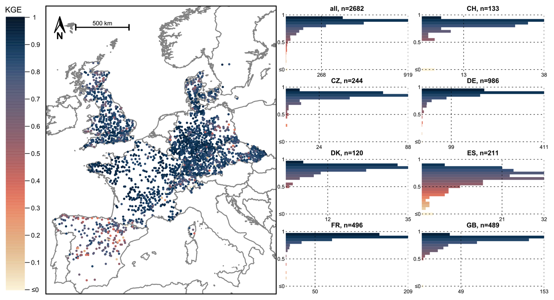
Figure 4 Model performance (Kling–Gupta efficiency, KGE) achieved for the 20 yr period between October 1995 and September 2015 when the E-OBS data obtained from EStreams were used for model calibration (scenario II). Note that the lower limit of the colour scale was cut at zero. Lower performances were plotted last to improve their visibility.

Considering the PBIAS as an additional measure for model performance (Fig. A4 for scenario I and Fig. 5 for scenario II), we found a small PBIAS (between −10 % and 10 %) for 2477 catchments for scenario I and 2468 catchments for scenario II (both 92 %). There were more occurrences of streamflow overestimations (i.e., positive PBIAS) when the CAMELS forcing data were used (scenario I) than when the E-OBS data were used: For 176 catchments (7 %), the PBIAS was larger than 10 %, and for 26 catchments (1 %), it was larger than 100 %. Meanwhile, a streamflow overestimation of at least 10 % only happened in 31 catchments (1 %) with the E-OBS forcing data (scenario II), but there was a considerable number of catchments for which the streamflow was underestimated (181 catchments (7 %) with a PBIAS smaller than −10 %).

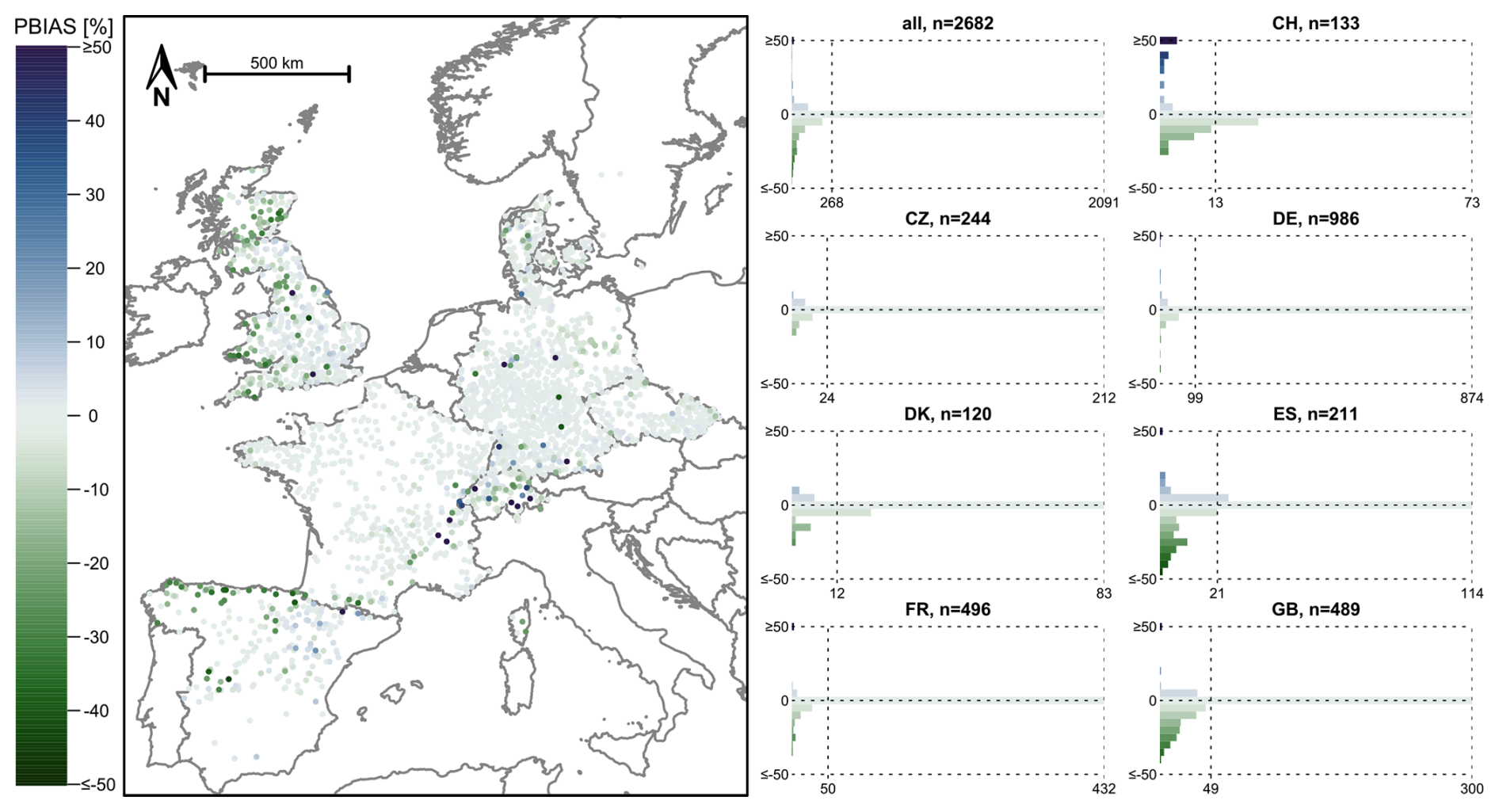
Figure 5 PBIAS (relative deviation of the simulated streamflow from the observed streamflow) for the 20 yr period between October 1995 and September 2015 when the E-OBS data obtained from EStreams were used for model calibration (scenario II). Note that the limits of the colour scale were cut at ±50 %. Largest deviations were plotted last to improve their visibility.

3.2.2 Differences in model performance between scenario II and I

To directly assess the differences in model performances between scenario II and I, we looked at the performance differences (Fig. 6). For 1669 catchments (62 %), model performances were (at least slightly) higher when the CAMELS data were used (scenario I), while for the other 38 % of all catchments, the use of E-OBS data resulted in better model performances. The strongest regional differences were found for the catchments in Spain and Great Britain.

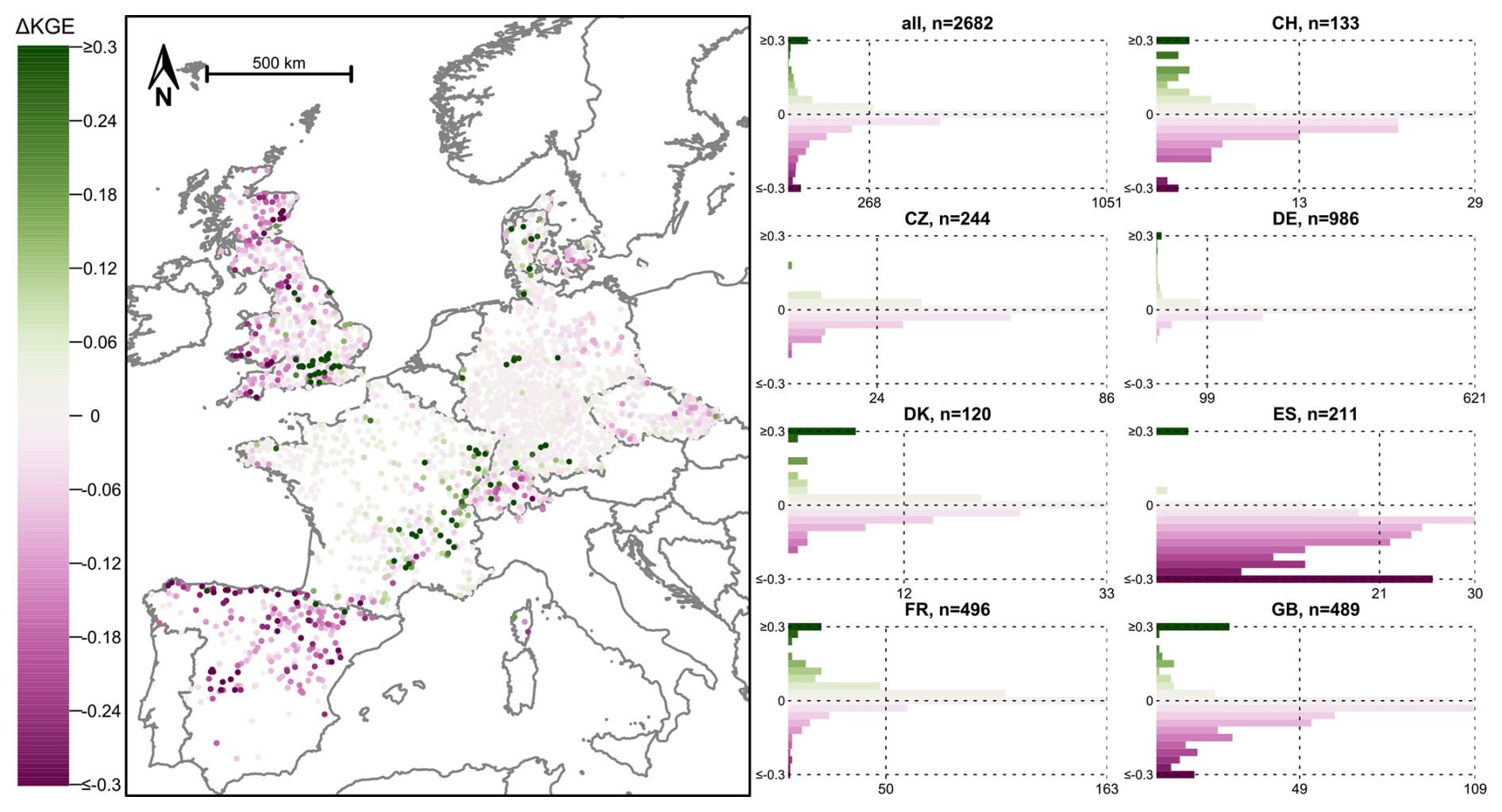
Figure 6 Difference in model performance (Kling–Gupta efficiency, KGE) between scenario II and scenario I. Positive values and green colours indicate higher performances when the E-OBS data obtained from EStreams were used, negative values and pink colours indicate higher performances when the CAMELS data were used. For the model performances, see Figs. 4 and A3. The catchments with the largest differences (in absolute terms) were plotted last to improve their visibility. Note that the colour scale was cut at ±0.3.

For France, there were notable improvements in model performance when using the E-OBS dataset: 316 catchments (64 %) had higher performances with the E-OBS data (median ΔKGE=0.01). Note that the French catchments that benefitted most from the E-OBS forcing data are the catchments for which the PBIAS was strongly positive when the CAMELS forcing data were used (scenario I; Fig. A4). For Sweden, all three catchments performed better with the E-OBS data, but the differences were very small (median ΔKGE=0.006; Fig. 6). For the catchments in Spain, it was the opposite: 200 catchments (95 %) performed better with the CAMELS dataset, reaching a median ΔKGE of −0.10. Higher KGE for scenario I was also observed for the catchments in Great Britain (80 %), Czechia (66 %), Switzerland (65 %), Denmark (61 %) and Germany (59 %).

The results also indicated some interesting intercountry patterns (Fig. 6). In France, the most considerable positive differences occurred for the catchments in the eastern, more mountainous part of the country, while for Great Britain, the CAMELS data resulted in clearly higher performances in most regions but not in the area around London.

3.2.3 Differences in model performance between scenario II and scenarios III, IV, and V

Replacing precipitation from E-OBS with data from CAMELS had by far the strongest impact on model performance (scenario III, Fig. A5). For most catchments, the performance differences between scenarios II and III closely mirrored the performance differences between scenarios II and I, indicating that precipitation accounted for a large share of the overall differences in performance. For only a few catchments (mostly in Great Britain), the performance gap between scenarios II and I was notably larger than between scenarios II and III. The opposite occurred for very few catchments (see Fig. S3 in the Supplement).

The effect of replacing the E_pot data (scenario IV) was quite limited. The higher E_pot data based on E-OBS were beneficial for a handful of catchments (ΔKGE>0.30 for 19 catchments), but the median difference was 0.00 (Fig. A6). Replacing only the temperature time series with the CAMELS data (scenario V) had virtually no effect on model performance for most catchments. There were no catchments for which the replacement of the temperature data increased the KGE by more than 0.10 and no catchments for which it decreased the KGE by more than −0.10 (see Fig. S4 in the Supplement). Note that only the temperature time series provided as input data to the HBV model were replaced, and not the data that were used to calculate E_pot.

3.3 Model performance linked to catchment attributes

We calculated the Spearman rank correlation between model performance and several catchment attributes available in EStreams (see Table S1 and Fig. S5 in the Supplement). The number of E-OBS precipitation stations and the aridity index emerged as particularly interesting variables given their apparent relationships with model performance.

3.3.1 Number of E-OBS precipitation stations

To assess the impact of the variable coverage of meteorological stations used to produce the gridded E-OBS dataset, we examined the relationships between the number of E-OBS stations within or near each catchment and the model performance for scenario II (i.e., using the E-OBS data contained in EStreams for all meteorological variables; see Fig. 4). Here, we present these relationship assessments per country (Fig. 7). The number of E-OBS precipitation stations was obtained from the EStreams dataset, defined as the count of stations located within a 10 km buffer of the catchment boundary (do Nascimento et al., 2024a).

Model performances for scenario II tended to be higher when more E-OBS stations were located in or around a catchment. Except for Sweden (for which we only considered three catchments), there was a significant positive correlation (p-value<0.05) between the station density and the model performances achieved with the E-OBS forcing data for all countries when all catchments were considered. To avoid that correlations are only due to a tendency for higher model performances in large catchments and more stations in large catchments, we also analysed the relationship for only the catchments smaller than 100 km². For Spain, the threshold was set to 500 km² due to the small number of catchments smaller than 100 km². There were still significant positive correlations for all countries, but not for Denmark and France. The correlations even increased for Switzerland (r=0.53 to r=0.71) and Great Britain (r=0.32 to r=0.36).

The performances were generally the lowest for areas with sparse station coverage, such as Spain and Great Britain (Fig. 7). However, low E-OBS station density did not always result in poor model performance. For catchments in France, Great Britain, Denmark, and Sweden, KGE values remained mostly above 0.5 despite a comparatively lower station density, suggesting that factors other than station density (such as the spatial variability of the rainfall due to topography or convective rainfall) also influence model accuracy. For additional insights, we also provide the scatterplots of the differences in model performance between scenarios II and I compared to the number of E-OBS stations per catchment (see Fig. S6 in the Supplement), which further supports this discussion.

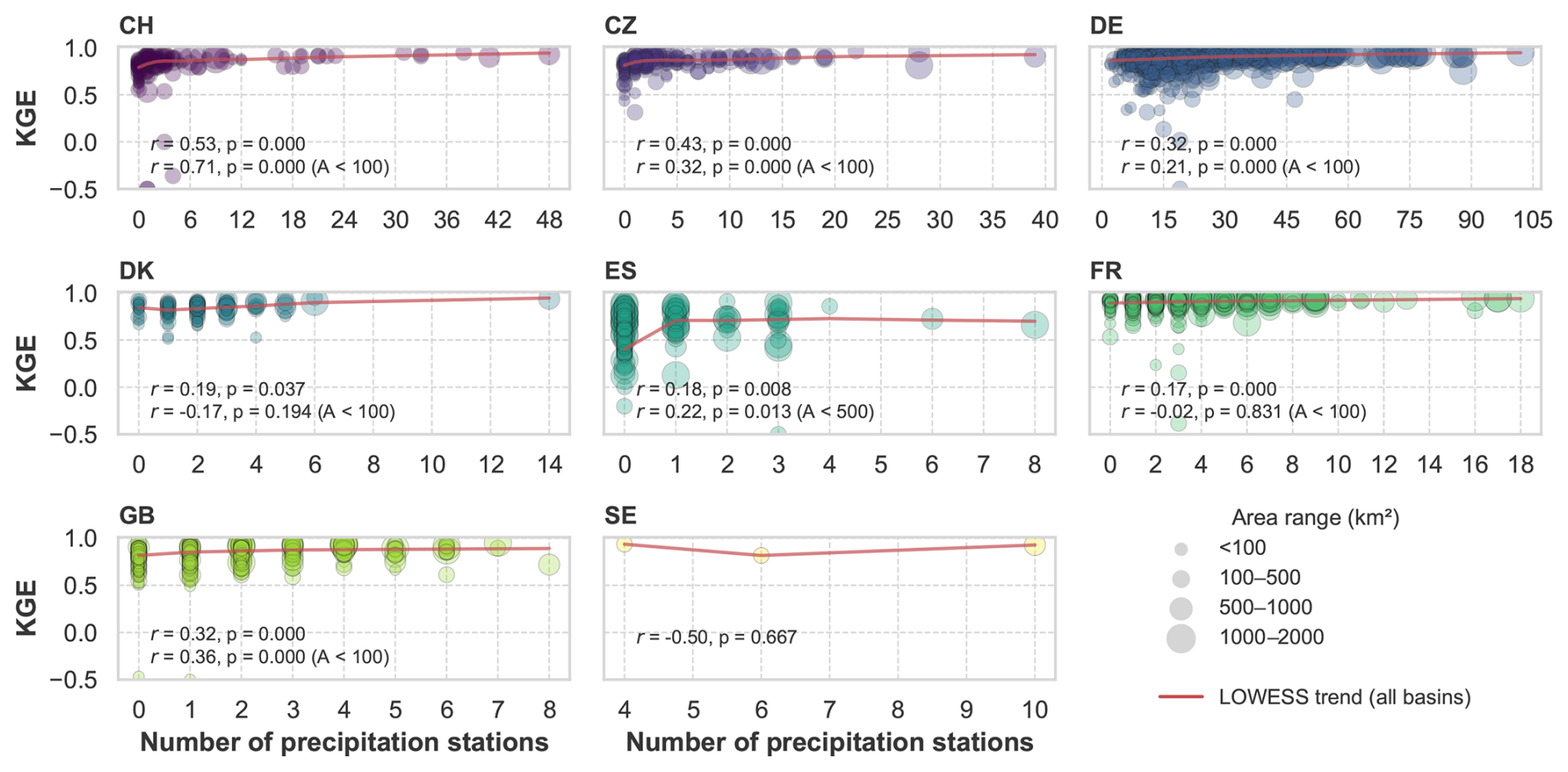
Figure 7 Scatterplots showing the model performance (Kling–Gupta efficiency, KGE) for scenario II (y axes) versus the number of E-OBS precipitation stations in and around each catchment, per country. Each circle represents one catchment, the size is based on catchment area. Each subplot contains the Spearman rank correlation (r) and corresponding p-value, and the lowess trend line. The r and the p-value are computed for all catchments per country and also for the ones with an area below 100 km² (500 km² for Spain). Note that the y axes were cut at −0.5, and the x axes differ for the different subplots.

3.3.2 Aridity index

We also evaluated the model performances for scenarios I and II in relation to the aridity indices derived from the respective forcing data (Fig. 8). Despite some atypical cases (Denmark in scenario I and Great Britain in scenario II), the model performances tended to be significantly lower in catchments with higher aridity indices (drier catchments). This trend was particularly evident for the catchments in Czechia, Germany, Spain, and Great Britain. Although the pattern appeared with both forcing datasets, it was more pronounced for the CAMELS data (scenario I), especially for the catchments in Czechia, and Spain (both with $r=-\mathrm{0.48}$). For Switzerland and France, the Spearman rank correlations were non-significant and close to zero for both forcing data types.

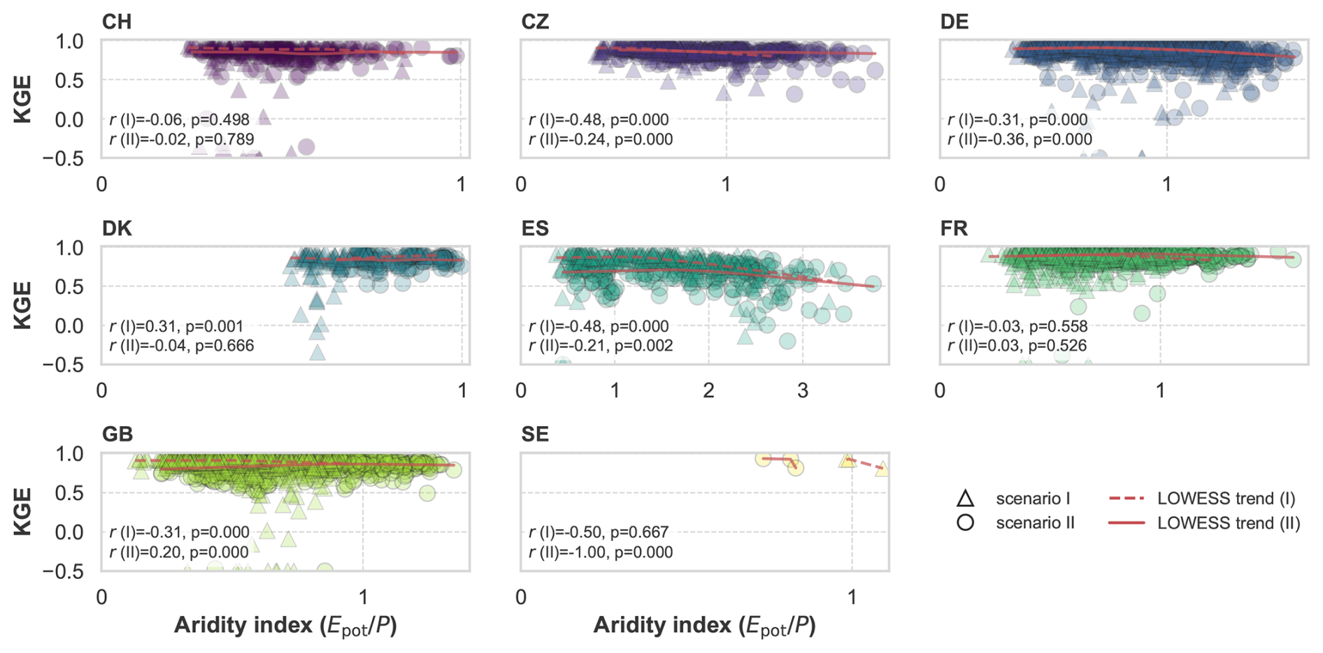
Figure 8 Scatterplots showing the model performance (Kling–Gupta efficiency, KGE) for scenario I and II (y axes) versus the aridity indices derived from the corresponding forcing data (CAMELS for scenario I, E-OBS from EStreams for scenario II), per country. Each subplot contains the Spearman rank correlation (r) and corresponding p-value, and the lowess trend line. Note that the y axes were cut at −0.5. Note that the x axes differ for the different subplots.

4 Discussion

4.1 Differences in the meteorological data

Our results show that the mean annual precipitation sums in E-OBS are systematically lower than those in the CAMELS datasets for most catchments (Sect. 3.1), with the largest differences occurring in Spain, whereas the smallest deviations were found in Germany (Fig. 1). This pattern is consistent with the findings of Bandhauer et al. (2022), who showed that E-OBS tends to underestimate precipitation to smooth spatial contrasts in comparison to a reference dataset, particularly in mountainous regions and in areas with sparse station coverage. In contrast, where E-OBS is supported by dense observation networks, such as in Germany, precipitation contrasts were better represented and the agreement with reference datasets was substantially improved (Bandhauer et al., 2022). Taken together, this suggests that the lower precipitation estimates in E-OBS relative to CAMELS are largely driven by the combination of coarser grid-resolution and lower underlying station density, especially in complex terrain. By contrast, mean temperatures from E-OBS and mean annual E_pot were generally higher than those from the CAMELS forcings (Fig. 2). We do not have a clear explanation for this behaviour, but potential reasonings are homogenization procedures, elevation corrections, and interpolation methods used in the different national datasets, which is beyond the scope of this study. The difference in E_pot is likely driven by the differences in temperature and may be further amplified by differences in the E_pot formulations and parameterizations used in the different products. The differences between the two forcing sources are the smallest in Germany also for E_pot, where there is both higher E-OBS station density, and a similar equation used for E_pot derivation in CAMELS to the one in E-OBS (Table 2).

4.2 Model performances

The HBV model is known for its capabilities in simulating streamflow, particularly in humid catchments, where water flow is related to varying soil saturation and hydrological connectivity (Knapp et al., 2022, 2024). This, in part, seems to explain the consistently high model performances achieved using either the CAMELS or the E-OBS forcing data (Figs. 4 and A3 as well as Figs. 5 and A4) for the more humid catchments, such as those in Sweden and Denmark. In contrast, in Spain, where the most arid catchments are located, the KGE values were the lowest and most variable for both scenarios. These findings are reinforced by the observed relationship between model performance and the aridity index shown in Fig. 8. The trend of decreasing performance with increasing aridity further supports the assertion that arid catchments pose significant challenges for hydrological modelling. Several other studies have suggested that for dry catchments more complex model structures may be needed for streamflow simulation, and even then, they still tend to yield lower model performance (Atkinson et al., 2002; David et al., 2022; Massmann, 2020).

Yet, the lower model performance for the catchments in Spain may be attributed not only to the inherent complexities of streamflow generation in arid environments, but also to the higher variability and limited availability of observational hydrometeorological data in these regions, which complicates model calibration and validation, as noted in previous studies (do Nascimento et al., 2024b; Yu et al., 2011). Additionally, previous studies have pointed out that many Spanish catchments, including the ones available in the currently used BULL dataset, are highly regulated, with dams and diversions (Klotz et al., 2025; Senent-Aparicio et al., 2024b). Although we purposefully adopted the criteria based on the number of lakes, and normalized upstream capacity area discussed in Sect. 2.1, some of these heavily modified catchments may still not be adequately filtered out, thereby further impairing overall model performance.

4.3 Influence of forcing data characteristics on model performance

Our findings indicate that model performance in scenario II is strongly influenced by the density of stations used to obtain the E-OBS data (see Sect. 3.3.1). As a result, the reliability of model outputs varies considerably across regions – an observation that is consistent with previous research (Klotz et al., 2025). This spatial dependency is visually supported by Fig. 6 in the EStreams paper by do Nascimento et al. (2024a), which shows the density of E-OBS stations across Europe. Notably, for regions with a high density of stations, such as Germany, the model achieved the highest KGE values with E-OBS data, underscoring the critical role of data availability and quality in hydrological modelling accuracy. Importantly, the significant correlations also found on smaller catchments (Fig. 7) confirmed that this relationship is not just an artifact of catchment size. To further understand the regional variations in model performance, we also examined how the type and characteristics of the CAMELS forcing data varied across countries, extending the comparison to both scenario I and II. This comparison provides insights into the role of data resolution, origin, and processing methodology in shaping the current model outcomes.

Germany presents a particularly consistent case: E-OBS shows high station density over the country (Fig. 6 in do Nascimento et al., 2024a), likely overlapping with the ground observations used in the national HYRAS dataset (Rauthe et al., 2013; Razafimaharo et al., 2020), which explains the high agreement between the precipitation forcings (Fig. 1) and the similar model accuracy obtained with both input datasets (Fig. 6). Minor discrepancies are expected, given HYRAS's finer spatial resolution (1 km for precipitation, 5 km for temperature) compared to E-OBS (0.1°).

In contrast, the national products for Spain, Switzerland, and Great Britain are based on substantially denser station networks than E-OBS (Table 2), which likely contributes to their higher model accuracy in scenario I relative to scenario II. As shown in Fig. 6 by do Nascimento et al. (2024a), E-OBS displays sparse station coverage in these countries. At the same time, it is worth noting that their respective national datasets – AEMET (5 km), RhiresD/TabsD (2 km), and CEH-GEAR/CHESS (1 km) – offer much finer spatial detail, which likely offer a better local representation of forcing patterns.

The meteorological data in the CAMELS of Denmark and France stand out for their coarser spatial resolution (10 and 8 km) compared to the other CAMELS datasets. In Denmark, this likely reduced the performance advantage of the CAMELS forcings, resulting in similar outcomes between scenarios I and II. In France, however, the situation differs: unlike the other CAMELS datasets, the SAFRAN product combines reanalysis and station-based data (Quintana-Seguí et al., 2008; Vidal et al., 2010). The KGE performances in scenario II being slightly better in 64 % of the French basins might suggest that SAFRAN's reanalysis nature, alongside coarser gridded-resolution, may explain the marginally lower accuracy relative to the purely station-based E-OBS forcing. However, note that the lower precipitation data and higher E_pot data in E-OBS compared to CAMELS-FR can also just be advantageous for model calibration, e.g., if there are additional outflows from the catchments that are not represented in the model structure (see Sect. 4.4 for further discussion).

For Czechia, the CAMELS forcings resulted in clearly better model performances than the E-OBS forcings, consistent with its high-resolution station-based dataset, while Sweden, represented by only three catchments, provides insufficient evidence for interpretation.

Overall, these results indicate that differences in model performance seem to be mainly driven by the station density used to derive the forcing, spatial resolution, and type of the product (station-based or reanalysis), leading to variability in the data quality even within the same source.

4.4 Influence of different E_pot data in model performance

In this work, the differences in model performance across the various sources of forcing data were mainly attributed to the differences in precipitation inputs (scenario III), whereas discrepancies in E_pot and temperature data hardly affected model performance (scenarios IV and V). These findings are consistent with those of Clerc-Schwarzenbach et al. (2024), who compared the Caravan and CAMELS datasets. Although their analysis revealed larger differences in E_pot than in precipitation data, it was still the precipitation inputs that exerted the greatest influence on model performance.

In this study, the differences between the E_pot data derived from E-OBS and the E_pot data derived from the CAMELS datasets were much smaller, but still obvious (which makes sense, considering the differences in the temperature data that were generally used as input to the E_pot calculations). This demonstrates once again the large uncertainties that we face when using different approaches to estimate E_pot. Several studies have already identified this issue as a persistent “blind spot” in hydrological modelling (Bai et al., 2016; Federer et al., 1996; Hanselmann et al., 2024). Nevertheless, E_pot calculated with the Hargreaves equation, as in EStreams, has been found to be a reliable method in various hydrological modelling applications, including in Central Europe (Pimentel et al., 2023), Germany (Loritz et al., 2024) and other regions (Bangi and Soraganvi, 2023; Sperna Weiland et al., 2012). Furthermore, as shown in Fig. A6, the differences in E_pot data did not affect model performance results strongly, so it can be expected that the use of a different equation would not notably change the findings of this study.

While the different E_pot data had a very limited effect on model performances in general, the higher E_pot data derived from E-OBS were beneficial for the model performance in some cases, as they likely allowed the model more flexibility to adjust the water balance. For example, the low performances with the CAMELS-GB data for the catchments in the karstic area around London can (partially) be explained by the inability of the HBV model to simulate groundwater losses (Lane et al., 2019; Oldham et al., 2023; Seibert et al., 2018). In such catchments, the higher E_pot values from E-OBS effectively helped to improve the water balance by allowing for more evaporation, thereby compensating for the unmodelled groundwater losses. This is supported by the fact that the strong streamflow overestimation in this and other regions (e.g., southeastern France) when the CAMELS forcing data were used (Fig. A4) could be avoided when the E-OBS forcing data were used (Fig. 5). However, it is important to note that while this adjustment led to improved model performance, such compensatory effects are not desirable when the objective is to accurately represent internal catchment processes. Achieving realistic process representation should, generally, remain a central goal in hydrological modelling (Kirchner, 2006).

4.5 Limitations

As mentioned with the example of the compensation effects due to higher E_pot data, a higher model performance does not necessarily mean a better representation of the hydrological processes. Still, we used the performance as an indicator for the hydrological efficacy of different forcing data. Although model performances are often used as an aggregated measure of data quality (Beck et al., 2017; Clerc-Schwarzenbach et al., 2024; Tarek et al., 2020), model performance can also be heavily influenced by the chosen model structure, particularly if it does not align well with the physical characteristics of a given catchment. This structural sensitivity means that performance differences may reflect model limitations as much as data quality (Beven, 2018).

Beyond model structure, it is worth noting that here we performed single-basin calibrations. While this allows for localized optimization, it does not reflect how models are typically regionalized for prediction in ungauged basins. Future research should explore how the identified performance patterns translate to a regionalization framework, which would provide more practical insights for prediction in data-scarce environments, and therefore, where model calibration is not possible.

Finally, all simulations in this study were conducted at a daily time step. For smaller catchments, a finer temporal resolution, such as hourly, could provide more meaningful insights. With the increasing availability of temporally high-resolution datasets (Coxon et al., 2025; Dolich et al., 2025; Nijzink et al., 2025), future studies may benefit from repeating similar analyses at the sub-daily timescale.

5 Conclusions

In this study, we compared the meteorological time series for 2682 European catchments in the EStreams dataset with time series from eight smaller-scale datasets (mostly CAMELS datasets). Moreover, we evaluated how the different types of meteorological forcing data influence the performance of a bucket-type hydrological model.

Our results showed that for most catchments, mean annual precipitation values obtained from the E-OBS dataset were lower than those from the corresponding CAMELS datasets. The opposite was true for the average temperature and thus the annual sums of E_pot (higher values in E-OBS than in CAMELS). These discrepancies led to consistently higher aridity indices computed with the E-OBS data in comparison to the CAMELS data for most catchments, although the spatial pattern remained similar. Such systematic differences highlight important inconsistencies across the two data sources that can affect the outcomes of hydrological synthesis studies across large areas.

Despite these differences, model calibration using either set of forcing data achieved good model performances for most catchments (KGE of at least 0.70 in more than 90 % of the catchments). However, performances were generally slightly lower when using E-OBS data than when using CAMELS data: For approximately 60 % of the catchments, the model performance was higher when using CAMELS forcing data. Considering the national curation and higher resolution of the CAMELS datasets, this makes sense.

Our findings indicate that cross-country differences in model performance are primarily driven by variations in station density, spatial resolution, and the inclusion of reanalysis components, rather than by substantial inconsistencies in data quality between E-OBS and national products. We observed that model performances using E-OBS forcing data were lower in regions with a lower E-OBS station density. This highlights the critical role of station coverage on hydrological model performance, an issue that becomes even more pronounced in mountainous regions, where steep climatic gradients in precipitation and temperature make dense and spatially representative data essential for reliable simulations, as well as in arid regions and regions where convective rainfall is relevant.

Overall, while local or national datasets often yield the best model performances, our results suggest that the meteorological forcing data from E-OBS that is included in EStreams represents a valuable and harmonized alternative for pan-European studies. The advantage of E-OBS lies in its observational basis, consistent methodology, and coverage across all of Europe, making it especially useful when national datasets are unavailable or inconsistent. As such, E-OBS and EStreams provide a practical foundation for expanding large-sample hydrology beyond national boundaries while maintaining sufficient data quality for robust model applications.

Appendix A:  

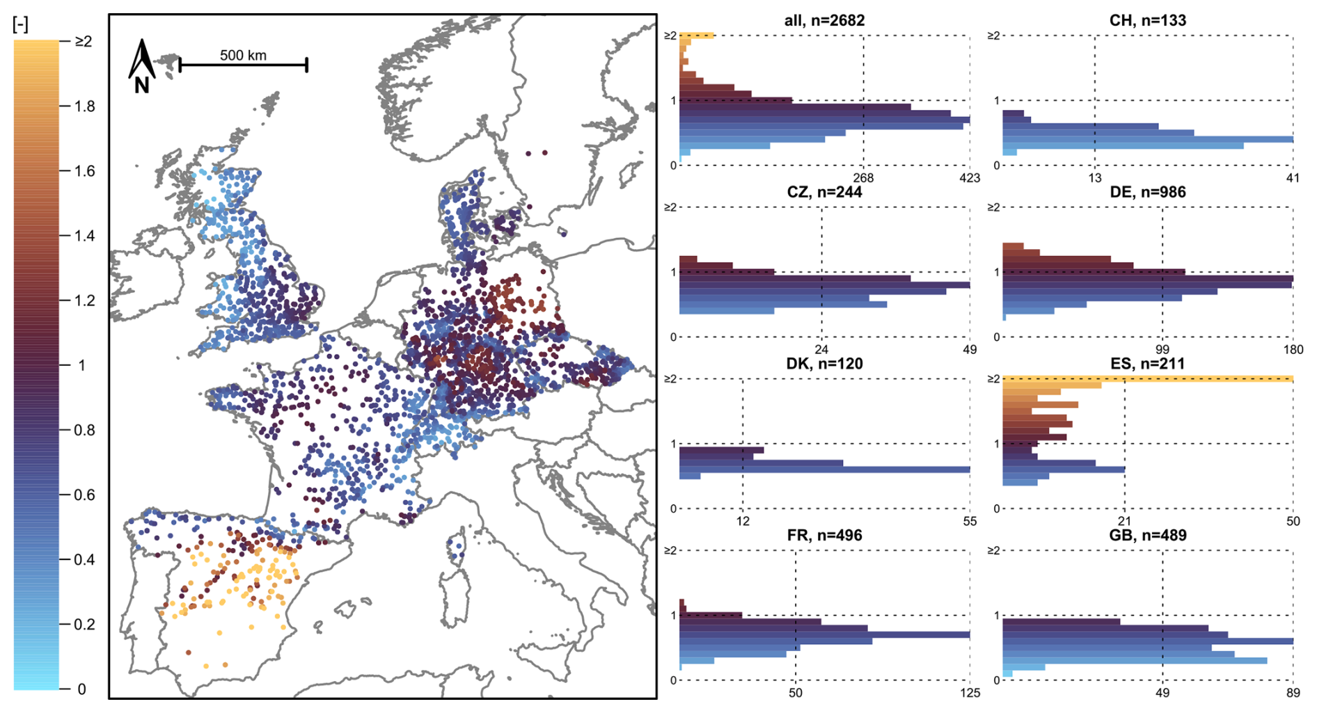
Figure A1 Aridity index ($E_{\text{pot}}/P$) calculated from the CAMELS data (for a 20 yr period: 1995–2015). Note that the colour scale was cut at a value of two.

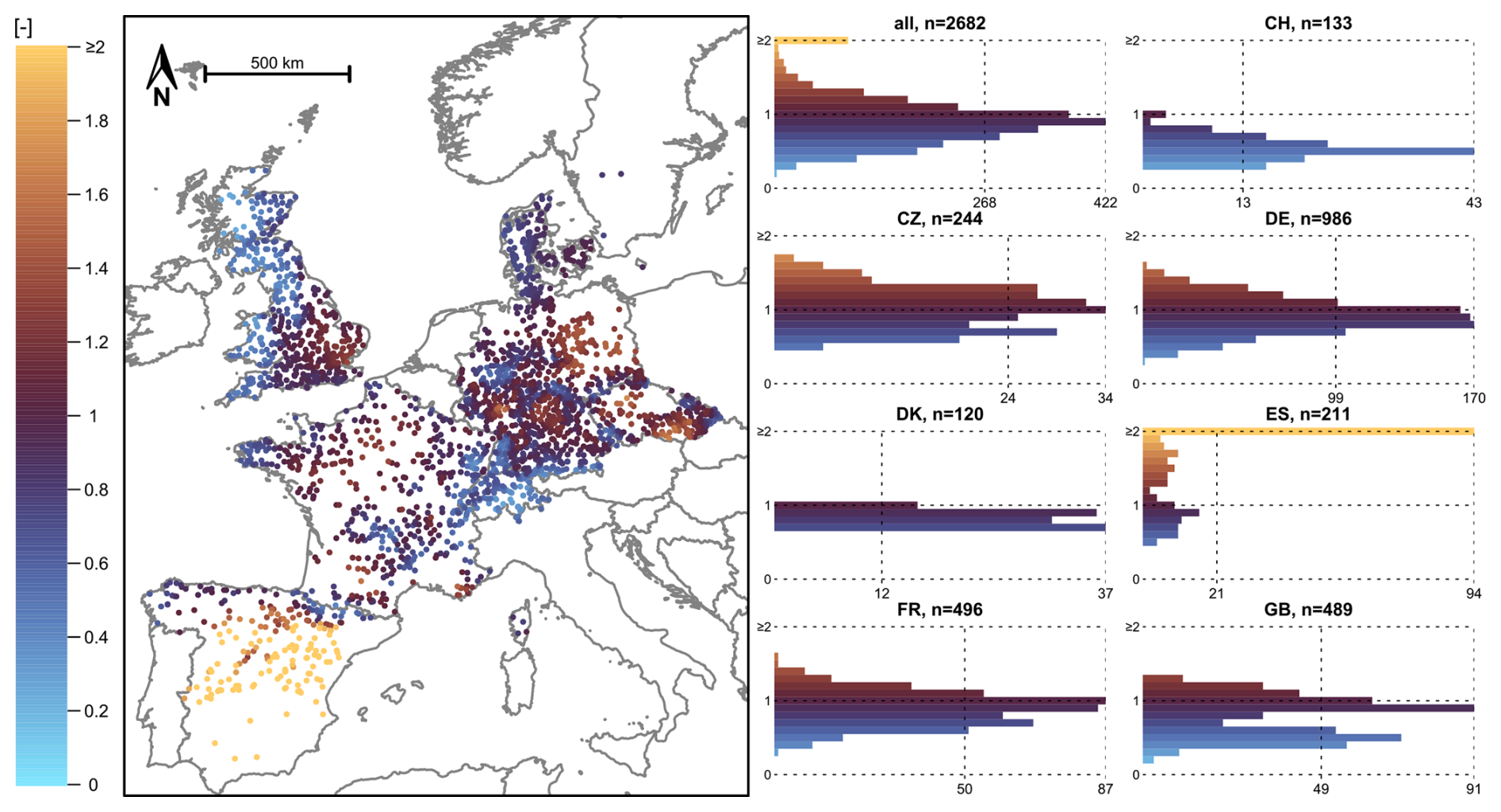
Figure A2 Aridity index ($E_{\text{pot}}/P$) calculated from the E-OBS data obtained from EStreams (for a 20 yr period: 1995–2015). Note that the colour scale was cut at a value of two.

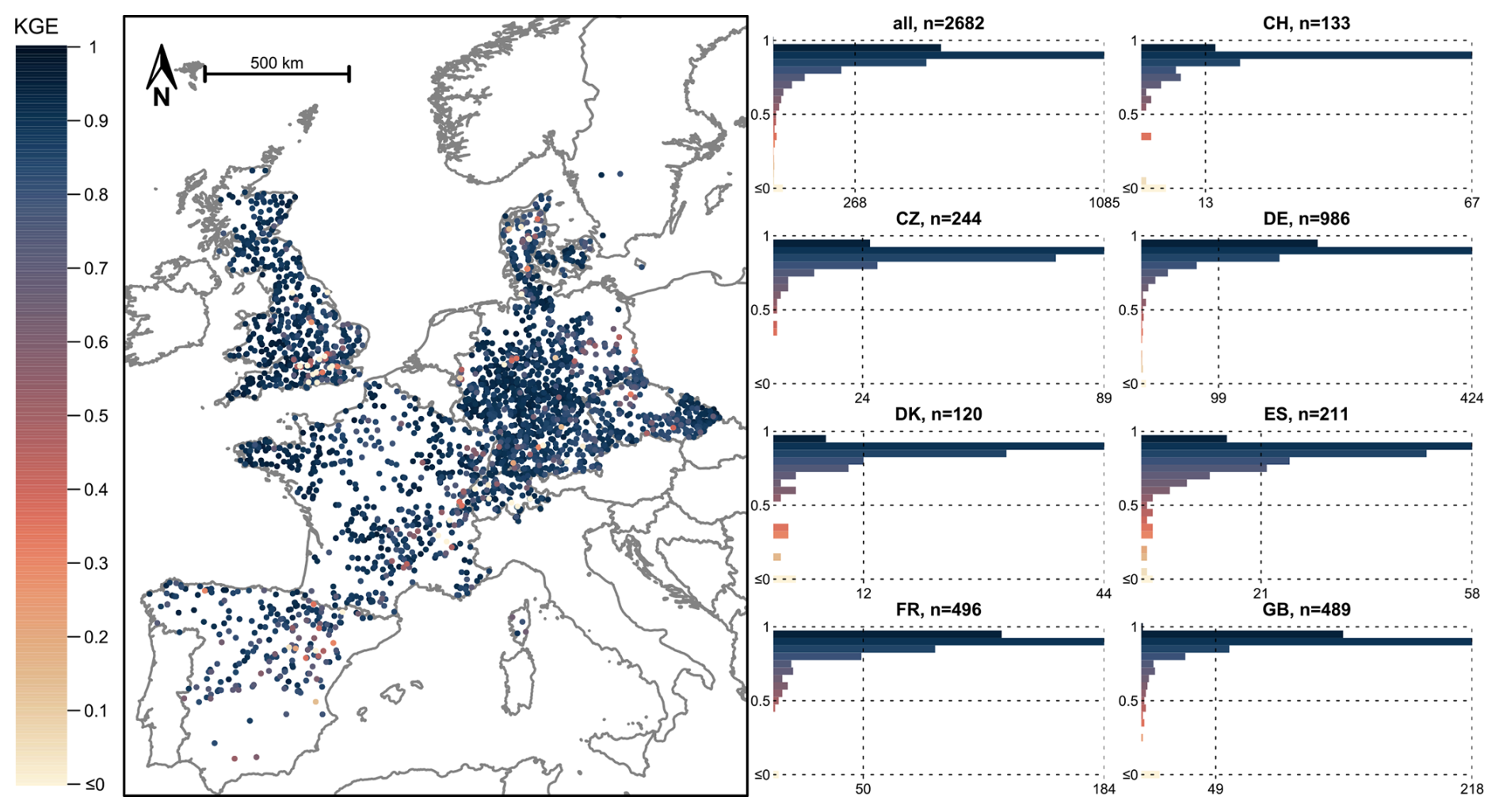
Figure A3 Model performance (Kling–Gupta efficiency, KGE) achieved for the 20 yr period between October 1995 and September 2015 when the input data from the CAMELS datasets were used for model calibration (scenario I). Note that the lower limit of the colour scale was cut at zero. Lower performances were plotted last to improve their visibility.

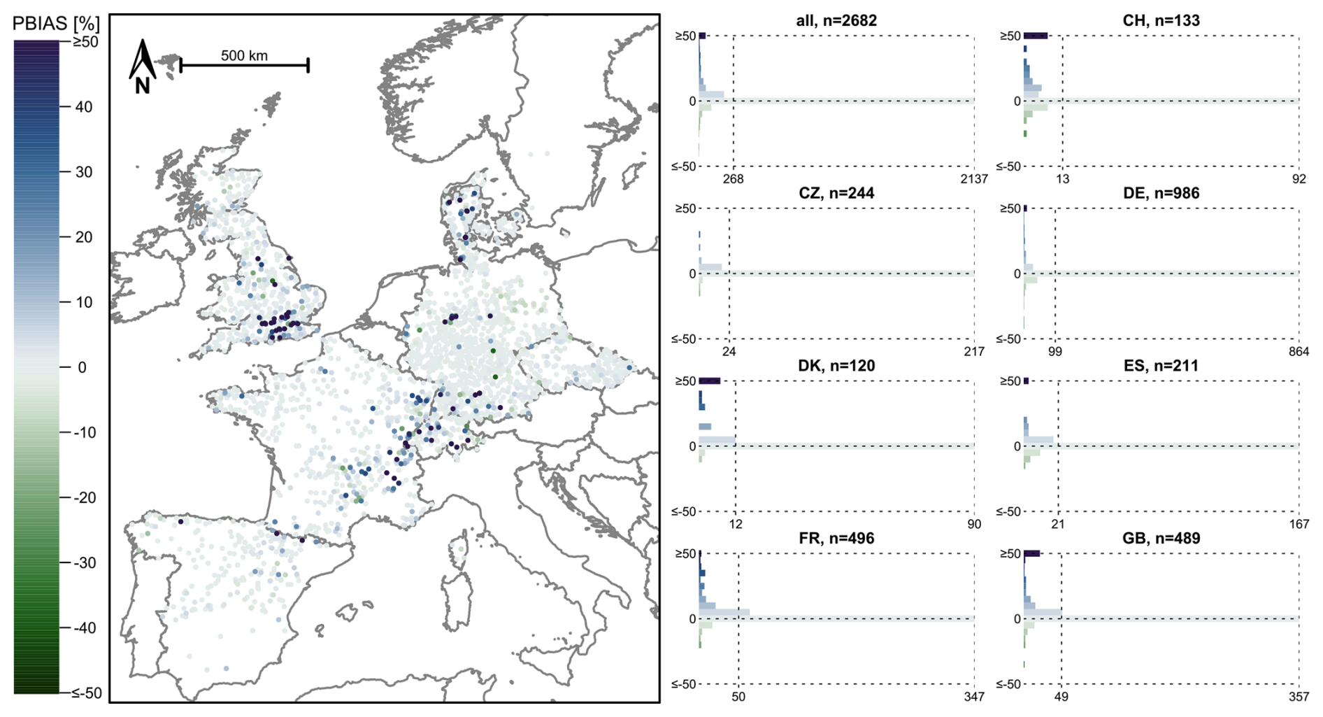
Figure A4 PBIAS (relative deviation of the simulated streamflow from the observed streamflow) for the 20 yr period between October 1995 and September 2015 when the CAMELS data were used for model calibration (scenario I). Note that the limits of the colour scale were cut at ±50 %. Largest deviations were plotted last to improve their visibility.

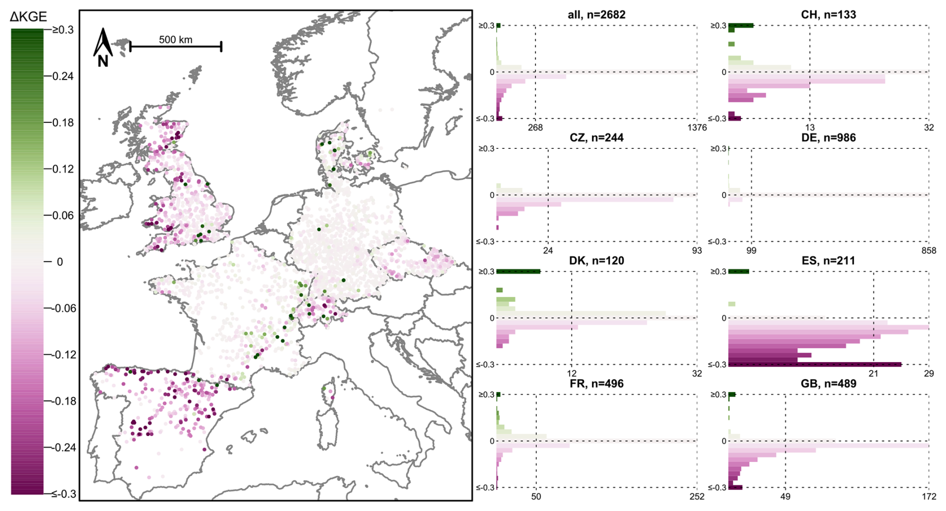
Figure A5 Difference in model performance when all meteorological input data were obtained from E-OBS (i.e., EStreams, scenario II) and when the precipitation data from E-OBS were replaced with those from CAMELS (scenario III). Positive values and green colours indicate higher model performances with the precipitation data from E-OBS, negative values and pink colours indicate higher model performances with the precipitation data from CAMELS. Note that the colour scale was cut at a difference in KGE of ±0.3. The catchments with the largest differences in model performance were plotted last to increase their visibility.

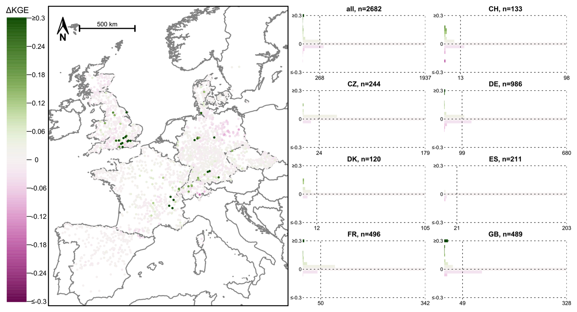
Figure A6 Difference in model performance when all meteorological input data were obtained from E-OBS (i.e., EStreams, scenario II) and when the E_pot data from E-OBS were replaced with those from CAMELS (scenario IV). Positive values and green colours indicate higher model performances with the E_pot data from E-OBS, negative values and pink colours indicate higher model performances with the E_pot data from CAMELS. Note that the colour scale was cut at a difference in KGE of $\pm \mathrm{0.3}.$ The catchments with the largest differences in model performance were plotted last to increase their visibility.