Lack of robustness of hydrological models: a large-sample diagnosis and an attempt to identify hydrological and climatic drivers

The transferability of hydrological models over contrasting climate conditions, also identified as model robustness, has been the subject of much research in recent decades. The occasional lack of robustness identified in such models is not only an operational challenge – since it affects the confidence that can be placed in projections of climate change impact – it also hints at possible deficiencies in the structures of these models. This paper presents a large-scale application of the robustness assessment test (RAT) for three hydrological models with different levels of complexity: GR6J, HYPE and MIKE SHE. The dataset comprises 352 catchments located in Denmark, France and Sweden. Our aim is to evaluate how robustness varies over the dataset and between models and whether the lack of robustness can be linked to some hydrological and/or climate characteristics of the catchments (thus providing a clue as to where to focus model improvement efforts). We show that, although the tested models are very different, they encounter similar robustness issues over the dataset. However, models do not necessarily lack robustness in the same catchments and are not sensitive to the same hydrological characteristics. This work highlights the applicability of the RAT regardless of model type and its ability to provide a detailed diagnostic evaluation of model robustness issues.

1 Introduction

1.1 Hydrological modelling under climate change

Several recent international initiatives have raised concerns about the issue of model robustness in hydrology. By model robustness we mean the ability of a hydrological model to adapt to contrasting climate conditions. For example, the Panta Rhei decade of the International Association of Hydrological Sciences (IAHS) (Montanari et al., 2013) and the Unsolved Problems in Hydrology (UPH) initiative of Blöschl et al. (2019) (see e.g. UPH no. 19: How can hydrological models be adapted to be able to extrapolate to changing conditions?) questioned the applicability of hydrological models in the context of global change. In parallel, a large number of hydrological modelling studies have been carried out to understand how climate change impacts hydrology (see e.g. the Intergovernmental Panel on Climate Change – IPCC – and Pachauri et al., 2014), and it seems essential to verify that the models used for this purpose withstand non-stationary climate conditions.

Over the past decade, several publications (e.g. Refsgaard et al., 2014; Thirel et al., 2015) have highlighted that hydrological models are not as independent of climate conditions as was expected. Indeed, models can be sensitive to the climate conditions of the period in which they were set up or calibrated (see e.g. Vaze et al., 2010; Coron et al., 2011). This dependency can be revealed using the split-sample-testing (SST) approach proposed by Klemeš (1986), which consists in testing the model on different time periods for calibration or evaluation (see Sect. 1.2). In split-sample experiments, model performance commonly decreases when switching from the calibration period to the evaluation period, and it has been shown that this decrease is intensified when the difference in climate conditions between periods increases (Brigode et al., 2013; Westra et al., 2014).

Different ad hoc solutions have been proposed to address this symptom. Varying the parameter values according to climate conditions is one such solution. For example, Gharari et al. (2013) proposed a method to calibrate time-consistent parameters based on the distance to the Pareto optimum, while other studies focused on time-variant parameters linked to climate conditions (Stephens et al., 2019; Zeng et al., 2019; Lan et al., 2020). Although these methods make it possible to improve robustness, they are not curative. That is, they serve as a “patch” for models that need to withstand changes in climate. They do not explain the reasons for the symptoms: why do model parameters exhibit this kind of unwanted dependence on climate, and why does this occur in some catchments and not in others?

1.2 Assessing model robustness from the perspective of a changing climate

In hydrological practice, model robustness has traditionally been assessed using SSTs (Klemeš, 1986). Klemeš (1986) introduced four levels of an SST, of which the third one, called a differential SST (DSST), aimed to evaluate a model over a period where the climate conditions differ from those of the calibration period. After a few early attempts to apply the DSST scheme (e.g. Refsgaard and Knudsen, 1996; Donnelly-Makowecki and Moore, 1999; Xu, 1999; Seibert, 2003), this test was more extensively used over the past decade to check the robustness of rainfall–runoff models in a changing climate (Vaze et al., 2010; Broderick et al., 2016; Dakhlaoui et al., 2017; Rau et al., 2019).

In addition, some authors proposed improvements to the DSST. Coron et al. (2012) suggested a generalized version of the SST (GSST) designed to evaluate models over all possible combinations of time periods. Gelfan and Millionshchikova (2018) introduced in the DSST a component that depends on model performance to avoid selecting apparently robust models with poor performances. Dakhlaoui et al. (2019) proposed a generalized differential SST (GDSST) by adding a bootstrap selection tool to create a number of contrasting climatic sub-periods. Gelfan et al. (2020) proposed a more complex evaluation strategy that uses a DSST in one step of the analysis. All of the aforementioned methods remain linked to the SST and include one or several calibration steps. However, the use of calibration and evaluation periods is not always suitable for assessing the robustness of models that are calibrated manually, that have complex calibration procedures or that even have no calibration at all.

When searching for a more widely applicable methodology, Nicolle et al. (2021) proposed a test inspired by the GSST of Coron et al. (2012) and by the subsequent work of Coron et al. (2014): the robustness assessment test (RAT). The RAT is designed to highlight unwanted correlations between climatic conditions and model performances, as these may represent an issue in modelling the hydrological cycle in a changing climate. The proposed RAT was found to give results similar to the GSST for catchments in France. In addition, the RAT has the major advantage of requiring only a single simulated flow time series (and an observed one for comparison): there is no need to resort to multiple calibration experiments. Therefore, the RAT can be used to compare the robustness of different models with minimal effort.

However, detecting cases where a model lacks robustness is not sufficient: we also need to understand the underlying reasons for this flaw. For example, Sleziak et al. (2018) used a DSST in Austria and identified an influence of land cover and catchment wetness on robustness. Birhanu et al. (2018) compared the model robustness of four models in order to evaluate how model complexity influences robustness. They concluded that catchment characteristics play a more important role in the lack of robustness than model complexity. However, it is often difficult to link the lack of robustness to model characteristics or to specific hydrological processes.

1.3 Scope of the paper

This paper aims to move a step forward in our understanding of what makes a model occasionally sensitive to climate change. The RAT (Nicolle et al., 2021) is applied to a set of 352 catchments spanning four Köppen climate classes (temperate and continental) in Denmark, France and Sweden, in order to evaluate the robustness of three rainfall–runoff models with various process representations and parameter estimation approaches (i.e. GR6J, HYPE and MIKE SHE). The large test set is used to evaluate how model robustness varies over a wide range of climatic and hydrological conditions and to characterize catchments where models lack robustness. The use of three different models will provide more general conclusions for characterizing catchments that raise robustness concerns in hydrological modelling.

2 Evaluation method

2.1 The RAT

The RAT (Nicolle et al., 2021) has been chosen since it can be applied without controlling the model calibration process. Indeed, the three models used for this experiment were calibrated once and separately at the three institutes involved in this study. The RAT only requires observed climatic variables (to be used as potential predictors for the model bias) as well as simulated and observed flows covering a sufficiently long time period (at least 20 years, as shown in the study by Nicolle et al., 2021).

Figure 1 summarizes the three steps of the RAT procedure: (i) the time series of the climatic predictors and flow are aggregated by hydrological year, (ii) a score assessing the difference between observed and simulated flows (here bias) is computed for each year and (iii) the correlation between this annual score and the annual values of a chosen predictor is analysed. A significant correlation between the score and the predictor will reveal suspicious dependencies that may affect the model's extrapolation capacity. We chose bias as the score with which to assess model error every year because we believe that it is the first metric to look at when looking at robustness in a climate change context. In this case, we will say for the sake of simplicity that the model “reacts” to the RAT for the catchment in question. Similarly, the catchment in which the model reacts will be termed a “reactive catchment”. Behind these terms, let us stress that the “reaction” is an unhealthy sign (it is definitely not what modellers aim for), and this does not tell us the causes of the behaviour, i.e. whether the issues are due to the model structure or parameters or to the presence of a trend in the observed data.

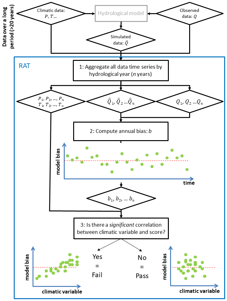
Figure 1 Flowchart of the robustness assessment test (RAT), with the three steps necessary to evaluate the robustness of a hydrological model (from Nicolle et al., 2021).

In this study, we consider hydrological years to be between 1 October and 30 September. The relative bias is computed every year between the observed and simulated flows (see Eq. 1 in Nicolle et al., 2021). Three climatic variables are used as potential predictors and compared with the bias: the annual mean air temperature (°C), the annual precipitation (mm yr⁻¹) and the annual value of the humidity index, which is the ratio between the annual precipitation and the annual potential evaporation (–). The correlation test is based on the Spearman correlation, so as to handle non-linear relationships. The significance threshold is set to a p value of 0.05.

2.2 Catchment set

The RAT is applied to a large catchment set over western and northern Europe (Fig. 2) to test the method and evaluate robustness over a variety of catchments. The dataset comprises a total of 352 catchments, of which 146 are located in France, 43 in Denmark and 163 in Sweden. The dataset was set up by the partners that collaborated in this work (INRAE in France, GEUS in Denmark and SMHI in Sweden). The catchment area varies from approximately 1 to 27 000 km² with a median of 530 km². The catchments cover a wide range of hydrological regimes (including contrasted or non-contrasted pluvial regimes, nival regimes and mixed regimes) and four Köppen–Geiger classes (Fig. 2; Cfb: temperate with no dry season and warm summers, Csb: temperate with dry and warm summers, Dfb: continental with dry and warm summers and Dfc: continental with dry and cold summers).

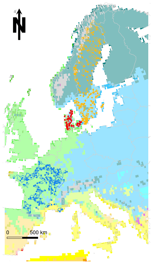
Figure 2 Locations and boundaries of the catchments used for this study. Background colours represent the Köppen–Geiger climate classes (the data and legend are described in Beck et al., 2018).

The hydrology of French rivers is under a double influence: geology and climate. The catchments located on the sedimentary deposits in the north and south-west are strongly buffered by the role of connected aquifers and are often strongly karstified in Jurassic plateaux. By comparison, the Hercynian granitic massifs (in central and western France) show a more classic hydrology typical of superficial catchments. In the Pyrenees, Alps, Jura and Vosges mountain ranges, hydrology can be heavily influenced by snowmelt. Around the Mediterranean Sea, and especially in the highlands, very heavy precipitation causes flash floods almost every autumn. The rest of the French territory has a rather mild (temperate) climate.

Swedish hydrology is characterized by decreasing air temperature from south to north and decreasing wetness from west to east. The highest runoff occurs in the mountain range along the western border with Norway, where the largest rivers originate, and also on the south-western coast. The south-east is rather dry. In terms of geology, Sweden is dominated by Precambrian crystalline and metamorphic rocks. Faults are one of the main factors that create topography and so influence catchment delineation. Most of the large rivers are developed for hydropower production, and water is stored in lakes and reservoirs for hydroelectricity production in the winter. We tried to avoid catchments that were too influenced by hydroelectricity production because this would have distorted the analysis: GR6J does not take any regulation into account. Sweden also has many lakes, which act as natural reservoirs.

In Denmark, hydrology varies from west to east. Geologically speaking, the western part of the Jutland peninsula (continental part of Denmark) is dominated by glacial outwash sand and gravel formations that are easily infiltrated by precipitation and that often form large inter-connected aquifers. The eastern part of Denmark is characterized by till and moraine deposits with a high clay content that are drained by tile drains and numerous smaller streams. As a result, fewer surface runoffs and other fast-flow components (drain flow) are generated in the western part compared to the eastern part. Therefore, streamflow in the western part of the country is dominated by baseflow, while overland flow is rarely an important flow component (van Roosmalen et al., 2007). By contrast, the catchments in the eastern part of Denmark are more responsive with more variable flow (Henriksen et al., 2021).

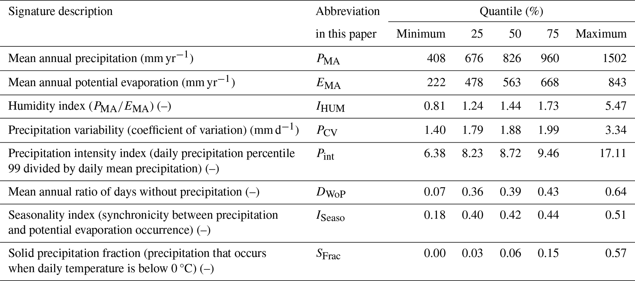
Several climate characteristics, named climatic signatures, were calculated for each catchment (see the statistics in Table 1). Repartitioning maps and distributions of these climate characteristics at a national scale are provided in Files S1 and S2 in the Supplement. Annual precipitation and potential evaporation show great variability over the dataset. The catchments with the highest amounts of precipitation are located in southern and eastern France, southern Denmark and western Sweden, while the catchments with the lowest precipitation amounts are mostly found in eastern Sweden. Regarding the humidity index, the catchments are all relatively humid, with the driest ones in south-eastern Sweden and in south-eastern and northern France. The indexes of precipitation variability and intensity are higher in eastern Sweden and south-eastern France and lower in western Sweden. The fraction of days without precipitation varies between 7 % and 64 % over the dataset; in half of the catchments the percentage of dry days is between 35 % and 45 %. This fraction is higher in south-eastern France and lower in northern Sweden. The seasonality index (de Lavenne and Andréassian, 2018) characterizing the synchronicity between precipitation and potential evaporation varies from 0.18 to 0.51. The lowest seasonality index values (mainly found in north-western Sweden) mean that runoff is favoured over potential evaporation, because precipitation mainly occurs when the evaporative demand is low. High seasonality index values, found in northern France and south-eastern Sweden, mean that potential evaporation is favoured. The snowfall fraction varies between 0 % and 57 % with a south–north gradient, but more than half of the catchments have less than 10 % snowfall. The distribution of climate characteristics by country provided in File S2 also shows that these characteristics vary greatly across France and Sweden. In Denmark, however, the distribution shows less spatial variability, with values around the average of the dataset.

Table 1 Distribution of climatic signatures over the catchment set (all three countries).

Statistics on flow signatures are compiled in Table 2, where most of the flow signatures are calculated following Westerberg and McMillan (2015). The repartitioning maps and distributions at the national scale of these flow characteristics are provided in Files S3 and S4, respectively. Mean flow varies from 95 to 1344 mm yr⁻¹, with low values in northern France and south-western Sweden and high values in western Sweden. Regarding the runoff ratio, values vary between 15 % and 124 %, with the highest values in northern Sweden and the lowest values in central France. Five catchments, located in the mountains of north-western Sweden, have values greater than 100 %. These values may be the result of an underestimation of the precipitation measurement due to orographic effects that are not captured by the interpolation method used.

Table 2 Descriptions and distributions of flow signatures over the catchment set (from Table 2 in Westerberg and McMillan, 2015). The abbreviations in column 2 are used in Sects. 3 and 4.

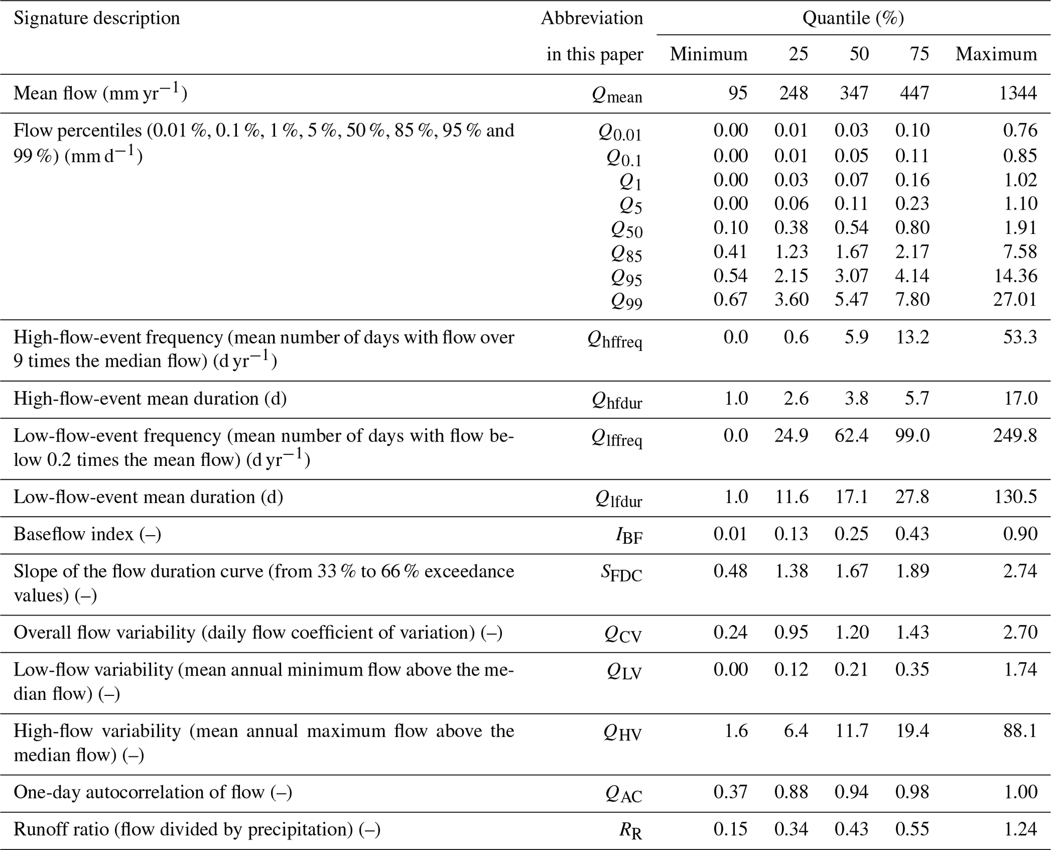
Low flows are characterized by several descriptors: the low percentiles (0.01 to 5), the frequency and duration of low-flow events, the baseflow index (I_BF from Pelletier and Andréassian, 2020) and the variability of low flows. Catchments with very low flows are located in southern and south-eastern Sweden and in central France. These catchments also have a low variability of low flows and a high frequency and duration of low-flow events. By contrast, catchments in continental Denmark (Jutland peninsula) and northern France are characterized by higher values of low flows that are more variable. The occurrence and duration of low-flow events are lower in these regions, and high I_BF values show that aquifers play a key role in the hydrology of these regions.

High flows are determined by high quantiles (85 to 99) as well as the frequency and duration of high-flow events and their variability. The values of high quantiles vary considerably over the dataset (e.g. Q₉₉ varies from 0.67 to 27 mm d⁻¹) and the highest values are located in western Sweden. Regarding the frequency and duration of high-flow events, no clear geographic pattern emerges. Flow variability is higher in France and lower in Denmark.

Finally, three signatures are computed to measure flow dynamics: the slope of the flow duration curve that evaluates flashiness, the overall flow variability and the 1 d autocorrelation. The slowest catchments are located in Denmark and northern France, while the fastest-responding catchments are found in south-eastern Sweden and south-eastern France.

The signatures listed in Tables 1 and 2 are used to investigate potential factors affecting the robustness of the three models tested. Catchments in which each model reacts to the RAT are compared with catchments where the model does not react. We use a Mann–Whitney U test (Wilcoxon, 1945; Mann and Whitney, 1947) to identify whether the distributions of the two signatures are significantly different (note that the same method was used, for example, by Fowler et al., 2016, to compare catchment characteristics). The Mann–Whitney U test evaluates the probability of two groups originating from the same distribution by focusing on the relative ranks of the groups. We use a classic (but nonetheless arbitrary) threshold for the p value: 0.05. These tests will allow us to target the robustness issues within the models and to better understand the RAT results.

2.3 Used data

For each catchment, daily precipitation, daily mean air temperature (referred to as “temperature” in this paper) and daily potential evaporation are available to run the models and to apply the RAT. For French catchments, temperature and precipitation are extracted from the SAFRAN reanalysis (Vidal et al., 2010). SAFRAN covers France on an 8 km grid and climatic data are aggregated by catchments (Delaigue et al., 2022). Potential evaporation is calculated using the formula proposed by Oudin et al. (2005). These data are available over 61 calendar years from 1958 to 2018. It should be noted that, for the interpretation of the results, the locations of ground stations used by SAFRAN to build the reanalysis can change over the available period and therefore have an impact on the model robustness. River flow data are available for each catchment outlet from the Banque HYDRO database (Leleu et al., 2014). Periods of flow data availability vary for each catchment: from 27 to 61 years between 1958 and 2018 with an average close to 50 years.

For Sweden, daily temperature, precipitation and observed flow are available for the same 35 calendar years from 1981 to 2016. Potential evaporation is also calculated for each catchment using the Oudin formula. Precipitation and temperature data are extracted from the PTHBV database (Johansson, 2002). This database covers Sweden on a 4 km grid and is based on extrapolation from measurement station data. River flow data for the 163 gauged stations are extracted from the official database of SMHI gauging stations. Meteorological data are available at a sub-catchment scale of an average size of 13 km² and are aggregated at the catchment scale.

For Danish catchments, data on precipitation, temperature, potential evaporation and flow are available for the same 30 calendar years from 1989 to 2019. A dynamic gauge catch correction (Stisen et al., 2011) is applied to the precipitation, and the results are subsequently interpolated to a 10 km grid (Scharling and Kern-Hansen, 2012). Potential evaporation is calculated using the Makkink equation adjusted for Danish conditions (Scharling, 1999). The Makkink equation is a global-radiation-based simplification of the Penman equation. Both temperature and potential evaporation are available at a 20 km grid resolution. Daily data on river flow are available from the national database ODA (surface water database; https://odaforalle.au.dk/main.aspx, last access: 31 December 2024). To minimize the correlation between the discharge time series, there are no nested catchments in the Danish dataset.

2.4 Hydrological models

The robustness of three models is evaluated in this work. The models were set up, calibrated and run by the three contributing groups of this work, according to their own expertise. Table 3 presents a brief description of the three models.

Table 3 Main characteristics of the three models used (OF: objective function).

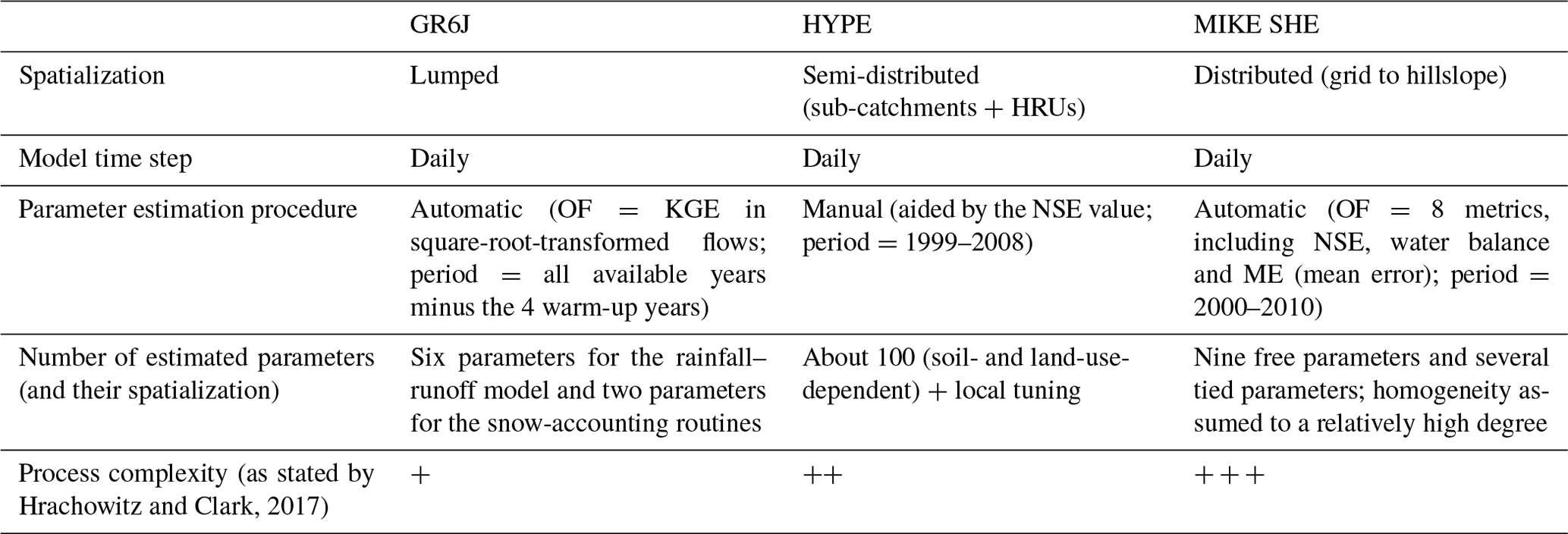
GR6J (Pushpalatha et al., 2011) is a lumped bucket-type model that simulates the catchment runoff response to rainfall using six free parameters which are adjusted during calibration. This model derives from the GR4J model (Perrin et al., 2003) and is run using the airGR R package (Coron et al., 2017, 2021). Snow accumulation and snowmelt are calculated using the CemaNeige routine (Valéry et al., 2014) that splits the catchment into five elevation bands and simulates snow processes with two additional parameters. The GR6J model is calibrated against the observed flow for each catchment using the Kling–Gupta efficiency (KGE) criterion (Gupta et al., 2009) calculated on square-root-transformed flows as an objective function. The calibration is done automatically using a mixed global–local search optimization algorithm presented by Coron et al. (2017). The period used for calibration covers all the available flow data minus a 4-year warm-up period to initialize the internal state variables (store levels). GR6J is the only model that we are able to apply to all the catchments of the dataset.

HYPE (Lindström et al., 2010) is a process-based semi-distributed model that was designed for both quantity and quality modelling. Here, we use it in Swedish catchments only, i.e. the Sweden-scale version (S-HYPE; Strömqvist et al., 2012). S-HYPE has been developed continuously since the first version described by Strömqvist et al. (2012). In the version used here (S-HYPE-2016b), the whole country is divided into sub-catchments of an average size of 13 km². These sub-catchments are divided into hydrological response units (HRUs) that depend on soil types and land uses. A large number of parameters are used to adapt the model and are spatialized by sub-catchments, land uses and soil types. Local super-parameters, i.e. deviations in key characteristics (see Lindström, 2016), are also calibrated for parameter regions in S-HYPE. Regulation of dams is taken into account using simple regulation rules. However, this module has a low impact on the results since the catchments used for this study are not affected by major dams. The S-HYPE model was calibrated manually. Since the model is used (among other things) operationally for flood warning at SMHI, the calibration was focused primarily on the timing of the discharge and secondly on the volume errors. The Nash–Sutcliffe efficiency (NSE) (Nash and Sutcliffe, 1970) is very sensitive to timing errors and was therefore used as the main numerical criterion in the calibration process. The results are available at https://www.smhi.se/data/hydrologi/vattenwebb (last access: 31 December 2024) for all Swedish catchments in the dataset for the entire period of flow data availability.

The MIKE SHE or MIKE 11 modelling system (Graham and Butts, 2005), only used for the Danish catchments, has a physically based and fully distributed description of the terrestrial hydrological cycle. It is based on a three-dimensional description of the saturated zone that is parameterized according to a geological model. Drainage flow is conceptualized as a linear reservoir assumed to occur when the water table is above the positions of the drains. The unsaturated zone is described by a simple water balance module termed the “two-layer” method. Evaporation is described by a simple method accounting for the water balance in the root zone. Two-dimensional overland flow is simulated using a diffusive wave approximation. Flow is simulated as a one-dimensional process by MIKE 11 using the kinematic routing approach. The model is discretized into a 500 m horizontal grid with 11 computational layers and is run with daily inputs on climatic forcing. More information on the model is found in the manual (DHI, MIKE SHE, User Guide and Reference Manual). For this work, the MIKE SHE version set up and applied by the National Water Resources Model (Højberg et al., 2013) is used. The model is calibrated using autocalibration provided by PEST (Højberg et al., 2013). Based on a sensitivity analysis, the most sensitive parameters are selected as free parameters, including hydraulic conductivities of the geological units, a drainage time constant, a river–aquifer exchange coefficient and the root depth of the dominant soil type. Several less sensitive parameters are tied to the free parameters.

As shown in Table 3, the three models have different process representations. They also have different spatial resolutions and different methods for parameter estimation. Since these three models cover various modelling approaches, they potentially have differences in robustness, and this work analyses how their structure influences their robustness.

3 Lessons learnt from a single model applied to the entire dataset

Out of the three models used in this paper, we were able to apply only one model, GR6J, to the entire dataset (because of its relative simplicity of calibration). The results of GR6J are therefore used to evaluate how robustness varies over the three countries studied. A geographic analysis is first carried out, followed by an analysis to link the occasional lack of robustness to catchment characteristics.

3.1 Overall evaluation

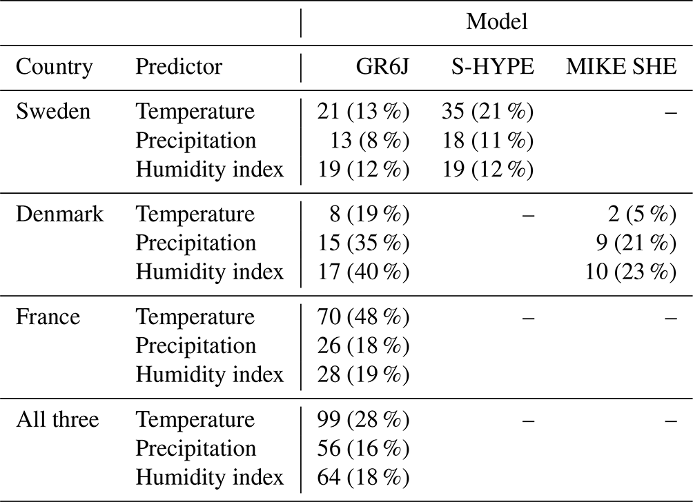
Figure 3 shows the locations and number of catchments where GR6J reacts to the RAT (i.e. a significant correlation exists between the bias and a given predictor) for the three predictors used (temperature, precipitation and humidity). When temperature is used as a predictor for the RAT, GR6J fails the robustness test over 99 catchments (28 % of the total). When precipitation and humidity index are considered, GR6J fails the robustness test in 16 % and 18 % of the catchment set. Note that these numbers are above the 5 % threshold that we would expect to observe if only chance were playing a role. This shows that the model has a significant robustness issue over the dataset.

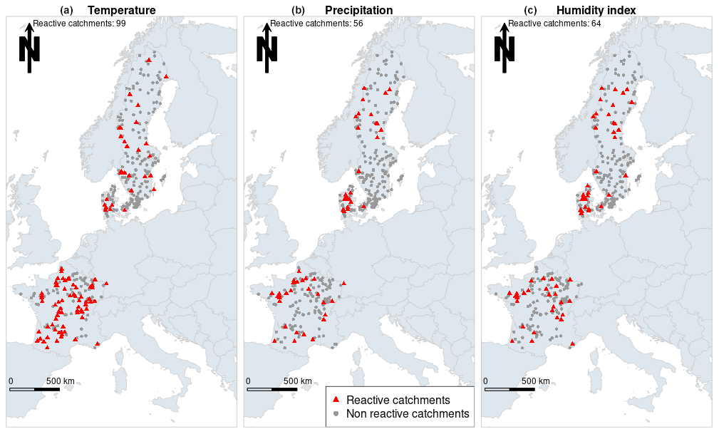
Figure 3 Locations of the catchments where GR6J reacts to the RAT (in red) using temperature (a), precipitation (b) and humidity index (c) as predictors. The numbers at the top of the maps represent the numbers of reactive catchments out of the total of 352 catchments.

The spatial distribution of the reactive catchments follows different patterns when temperature or precipitation is used as a predictor in the RAT. (i) When temperature is used as a predictor, 70 reactive catchments of a total of 99 are located in France. (ii) When sensitivity to precipitation is considered, there are fewer reactive catchments in France but more in Denmark. (iii) Results obtained with the humidity index and precipitation are very similar (this was expected because the humidity index is calculated as the ratio of the precipitation amount to the potential evaporation amount: since the annual variability of precipitation is much higher than the variability of potential evaporation, it is logical to observe similar results when the two variables are used as predictors).

Overall, the reactive catchments where GR6J is identified as lacking robustness are often grouped together geographically, which indicates that some common (regional) hydrological features cause this problem. For example, catchments react more often in the Jutland peninsula and in northern Sweden when precipitation or humidity index is used as a predictor.

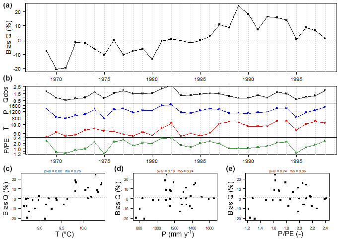
Figure 4 Illustration of the RAT results for the GR6J model applied to the Ognon River at Chavigny-sur-l'Ognon (north-eastern France): panel (a) represents the annual streamflow bias time series, the four middle plots in panel (b) represent the time series of the annual flow values and the three climatic predictors and the bottom scatterplots represent the correlation between the bias and annual temperature (c), precipitation (d) and humidity index (e).

However, we cannot identify any obvious reason for the spatial pattern of the reactive catchments. For example, it is not clear why so many reactive catchments are located in France when temperature is used as a predictor. An example of these is given in Fig. 4, in which the temperature is clearly correlated with the bias (bottom-left panel), while no clear correlation appears for the precipitation and humidity index time series (bottom-centre and bottom-right panels). One reason could be the higher values of potential evaporation in the country, which could explain a higher sensitivity to trends in temperature over time. The fact that data time series are longer in France does not seem to play a role, as the results are similar when the time period is reduced step by step from 40 to 20 years (not shown here).

The conclusion of this series of tests on GR6J is that the model seems to have robustness issues over the dataset but that, at this point, the RAT results cannot be explained by the locations of the reactive catchments alone. Thus, catchment characteristics are included in the analysis to evaluate whether robustness issues could possibly be explained by the specificities of local hydrology and whether this could be linked to the structure of the models.

3.2 Link to catchment hydro-climatic characteristics

In order to investigate potential factors affecting the robustness of the GR6J model, we analyse catchment characteristics. Catchments in which GR6J reacts to the RAT are compared with those where GR6J does not react to the RAT. Figure 5 shows an example of the methodology for mean annual precipitation over the catchment. The boxplot represents the distribution of mean annual precipitation, on the left for catchments where GR6J reacts to the RAT and on the right for catchments where GR6J does not react to the RAT. This shows that GR6J is less robust in the drier catchments (with temperature used as a predictor). For the precipitation and humidity index, no significant differences in mean annual precipitation exist between reactive catchments and non-reactive ones.

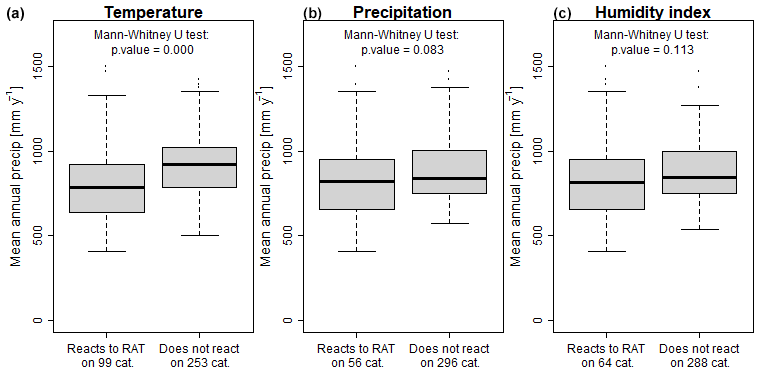
Figure 5 Comparison of the catchment area distribution for catchments where GR6J reacts or does not react to the RAT using temperature (a), precipitation (b) and humidity index (c) as predictors.

Following the same methodology, Fig. 6 shows the results of the Mann–Whitney U test described above for the climatic signatures listed in Table 1. It indicates those signatures for which the difference between reactive and non-reactive catchments is significant. If the colour is red (blue), the Mann–Whitney U test indicates that reactive catchments have lower (higher) values of the signature than non-reactive catchments. The shade of the dot colour indicates how significant the difference is: if it is grey, no significant difference exists (p value higher than 0.05); if it is dark red or blue, the difference is highly significant (p value lower than 0.01).

When temperature is the predictor, Fig. 6 shows that the catchments in which GR6J reacts to the RAT have higher precipitation and potential evaporation amounts and a higher number of dry days. The higher seasonality index indicates that precipitation mainly occurs during the low potential evaporation season (low synchronicity between high precipitation and high potential evaporation). The amount of precipitation that falls as snow is also lower than the dataset average.

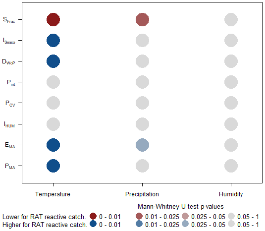
Figure 6 Results of the Mann–Whitney U test to evaluate the difference in climatic signatures (see Table 1) between catchments in which GR6J reacts to the RAT and catchments in which GR6J does not react. The number of catchments in each subset can be found in Fig. 5. Blue (red) circles mean that the signature is significantly higher (lower) for reactive catchments. P_MA: mean annual precipitation, E_MA: mean annual evaporation, I_HUM: humidity index, P_CV: precipitation variability, P_int: precipitation intensity index, D_WoP: ratio of days without precipitation, I_Seaso: seasonality index and S_Frac: snow fraction.

These results are not straightforward to interpret. The low synchronicity between precipitation and potential evaporation emphasized by the seasonality index values reveals that the reactive catchments have drier warm seasons (high potential evaporation and low-precipitation seasons). The reactive catchments are also mainly located in France, where potential evaporation is highest. The link between these two signatures may lead to dry seasons on which potential evaporation has a major impact. Given that potential evaporation is directly calculated from temperature, changes in temperature may influence hydrology during the warm season, and it is possible that GR6J has difficulties in handling these inter-annual changes in potential evaporation.

If either precipitation or humidity index is used as a predictor, the difference between the two distributions does not show a similar pattern. Lower differences in the climatic signature are evident between reactive and non-reactive catchments. The only discernible result is that, when precipitation is the predictor, catchments in which GR6J reacts to the RAT have less solid precipitation and/or a higher potential evaporation amount.

Consequently, it is difficult to find an explanation in terms of model representation based on climatic considerations, and therefore we now address flow signatures. We can only stress that the snow module is not the source of the lack of robustness here, since the snow fraction is lower for reactive catchments.

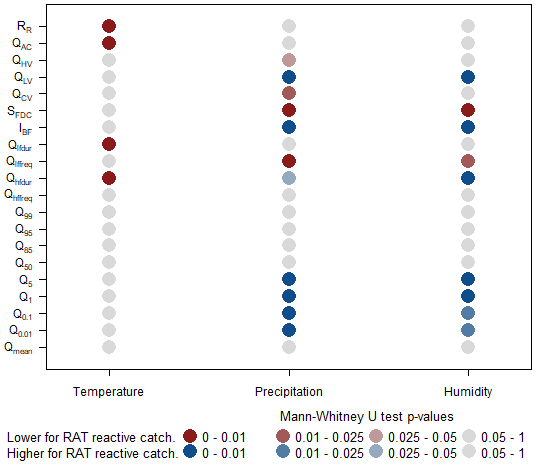
Figure 7 Results of the Mann–Whitney U test to evaluate the difference in the flow signature between catchments in which GR6J reacts to the RAT and catchments in which GR6J does not. The number of catchments in each subset can be found in Fig. 5. Blue (red) squares mean that the signature is significantly higher (lower) for reactive catchments. Q_mean: annual mean flow, Q_[0.01−99]: flow percentiles, Q_{[hf−lf]freq}: frequency of high- or low-flow events, Q_[hf−lf]dur: duration of high- or low-flow events, I_BF: baseflow index, S_FDC: slope of the flow duration curve, $Q_{[\mathrm{C}-\mathrm{L}-\mathrm{H}]\mathrm{V}}$: total low- or high-flow variability, Q_AC: flow 1 d autocorrelation and R_R: runoff ratio.

We now look at flow signatures to interpret robustness failures. Figure 7 complements the description of catchments in which GR6J reacts to the RAT. When temperature is used as a predictor, the reactive catchments are characterized by a low runoff ratio. The low autocorrelation and the short durations of low-flow and high-flow events suggest that the reactive catchments are more responsive than the dataset average.

Similarly to what was explained for Fig. 6, the low runoff ratio for reactive catchments indicates that potential evaporation may have more influence on these catchments.

When precipitation and the humidity index are used as predictors, low flows also seem to have relatively high values (Q_0.01 to Q₅ and high I_BF) and high variability in reactive catchments. Regarding the slope of the flow duration curves, the catchments that react to the RAT seem slower than average. Only when precipitation is the predictor are the total flow variability and high-flow variability also below normal.

The catchments with potential robustness issues are characterized by slow responses with high baseflow. Similar observations were made by Sleziak et al. (2018), who showed that the lack of robustness in Austrian catchments was higher for catchments with slow responses (“dominant soil moisture regime”). In the present work, this can be explained since, in this kind of catchment, the conditions of precipitation and humidity of a given year may influence flow during several subsequent years (possibly due to groundwater storage). It is known that GR6J has difficulties in representing this behaviour, described by de Lavenne et al. (2022) as the “catchment memory”. The RAT results suggest that this flaw in the model may lead to robustness issues.

To summarize, these evaluations do not lead to clear explanations of the lack of robustness of GR6J. However, two paths can be explored to improve its robustness: (i) when temperature changes over the catchment, the robustness of GR6J could be increased by improving its ability to handle inter-annual changes in potential evaporation; and (ii) when a precipitation trend impacts the catchment, the robustness of GR6J could be improved by better consideration of the catchment memory within the model.

4 Comparing model robustness in Denmark and Sweden

Here, we compare the robustness of the three models presented in Sect. 2.4. By applying the RAT to these models, our goal is to understand whether the catchments detected by the RAT as reactive are model-specific. In addition to this, we aim to highlight the differences between the models and try to interpret these differences.

4.1 S-HYPE vs. GR6J in Sweden

Figure 8 compares the catchments in which GR6J and S-HYPE react to the RAT in Sweden. The numbers of reactive catchments are similar for the two models, but their locations vary, even if some catchments are common to the two models. When temperature is used as the predictor, catchments in which S-HYPE reacts to the RAT are mainly located in the Scania region (extreme south of Sweden). Catchments in which GR6J reacts to the RAT are scattered over Sweden, but the large number observed for S-HYPE in Scania is not observed for GR6J. It is, however, interesting to note that catchments in central and western Sweden seem to present a robustness issue for both models. When precipitation and humidity index are taken as predictors, GR6J reacts in the northern regions, while S-HYPE reacts more in central and south-eastern Sweden. Overall, Fig. 8 shows that S-HYPE and GR6J react differently to the RAT and indicates that their lack of robustness probably has different origins.

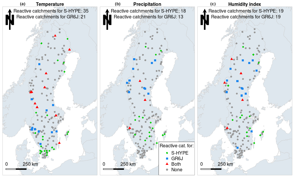
Figure 8 Locations and number of Swedish catchments in which S-HYPE and GR6J react to the RAT using temperature (a), precipitation (b) and humidity index (c) as predictors. The numbers at the top of the maps represent the numbers of reactive catchments out of 163 for each model.

Figure 9 compares how robustness is linked to catchment climate characteristics. The figure shows that there is a large difference in the catchment climate characteristics between HYPE and GR6J. GR6J reacts to the RAT for humid catchments with a higher number of rainy days, less aridity and lower potential evaporation. It is interesting to note that GR6J responds differently for Sweden than for the rest of the dataset, probably because of the specificity of Swedish hydrology (e.g. the influence of snow). Northern catchments seem to cause more robustness issues for GR6J. In these catchments, streamflow is regulated by hydroelectric power stations. Since regulation is not explicitly represented in the GR6J model, it is possible that this aspect of the catchment hydrology may lead to flaws in the models. Snow, which strongly influences hydrology in northern Sweden, may also be a reason for the issues in GR6J. The snow module that adds two parameters to be calibrated may then create robustness issues (even if this is not the case over the whole dataset).

Figure 9 Results of the Mann–Whitney U test to evaluate the differences in climatic signatures in Sweden. The left plot represents differences between Swedish catchments in which GR6J reacts and catchments in which it does not, and the right plot represents differences between catchments in which S-HYPE reacts to the RAT and catchments in which it does not. The number of catchments in each subset can be found in Fig. 8. Blue (red) squares mean that the signature is significantly higher (lower) for reactive catchments. P_MA: mean annual precipitation, E_MA: mean annual evaporation, I_HUM: humidity index, P_CV: precipitation variability, P_int: precipitation intensity index, D_WoP: ratio of days without precipitation, I_Seaso: seasonality index and S_Frac: snow fraction.

In the case of S-HYPE, where temperature is used as a predictor, reactive catchments seem to have a lower-than-average snow fraction and more potential evaporation. This is possibly due to the fact that latitude is not taken into account in the evaporation calculation in the HYPE model (the Oudin formula is not used in the model). This may lead to robustness issues in the catchments where evaporation has an impact. However, the significance is relatively weak, and no clear difference exists between reactive and non-reactive catchments: model robustness cannot really be linked to catchment characteristics.

Similarly to Fig. 9, Fig. 10 compares how the RAT results are linked to flow signatures for GR6J and S-HYPE. It also shows large differences in behaviour between the two models. When the precipitation and humidity index are taken as predictors, GR6J reacts for wet catchments with high flow and a high runoff ratio. This confirms the results from Fig. 9. GR6J seems to react to the RAT in specific types of catchments (which are large and have a higher-than-average specific flow). In these catchments, streamflows are more often regulated by human activities and, since there is no regulation module in GR6J (unlike in HYPE), this can create robustness issues in the model.

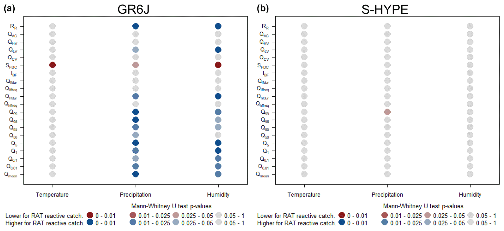
Figure 10 Results of the Mann–Whitney U test to evaluate the differences in flow signatures in Sweden. The left plot represents the differences between Swedish catchments in which GR6J reacts and catchments in which it does not, and the right plot represents the differences between catchments in which S-HYPE reacts to the RAT and catchments in which it does not. The number of catchments in each subset can be found in Fig. 8. Blue (red) squares mean that the signature is significantly higher (lower) for reactive catchments. Q_mean: annual mean flow, Q_[0.01−99]: flow percentiles, Q_{[hf−lf]freq}: frequency of high- and low-flow events, Q_[hf−lf]dur: duration of high- and low-flow events, I_BF: baseflow index, S_FDC: slope of the flow duration curve, $Q_{[\mathrm{C}-\mathrm{L}-\mathrm{H}]\mathrm{V}}$: total low- to high-flow variability, Q_AC: flow 1 d autocorrelation and R_R: runoff ratio.

For S-HYPE, again, no clear difference exists between reactive and non-reactive catchments. This result suggests that the HYPE model has robustness issues in random catchments (at least regarding the signatures evaluated here). One possible hypothesis to explain this could be that it is calibrated manually, often using super-parameters, and this may lead to different robustness issues for different locations. The choice of objective function (i.e. the NSE) and the focus on flood forecasting also led the modeller to place more emphasis on timing than on water balance, which could explain why the bias error is less significant for S-HYPE. The calibration procedure may lead to additional issues in terms of robustness that do not depend on catchment location or regime.

In summary, S-HYPE and GR6J have equivalent numbers of reactive catchments. Also, GR6J seems to behave differently in Sweden compared to France and Denmark, perhaps due to river regulations and higher snow fractions. It is very difficult to understand the issues found for S-HYPE since the reactive catchments do not differ significantly from the non-reactive ones. This could be due to the different calibration treatment of the model, which was calibrated manually and for a flood forecasting purpose. Since S-HYPE is calibrated primarily for flood forecasting, the long-term bias is taken into account for a second time, which may influence the RAT results for a catchment. Manual tuning specific to some catchments may introduce differences that make it difficult to identify a type of catchment that has robustness issues.

4.2 MIKE SHE vs. GR6J in Denmark

Figure 11 presents the catchments in which GR6J and MIKE SHE react to the RAT in Denmark. Overall, reactive catchments are mainly located in the Jutland peninsula (which corresponds to continental Denmark). In Denmark, unlike in Sweden and France, there are more reactive catchments when precipitation and humidity index are used as the predictors than when temperature is the predictor. However, as for the rest of the dataset, reactive catchments are almost the same when precipitation and humidity index are the predictors. The fact that MIKE SHE reacts to the RAT in fewer catchments than GR6J (13 vs. 22) shows that MIKE SHE is more robust than GR6J in Denmark. Despite this, there are several common reactive catchments between MIKE SHE and GR6J: 57 % of the catchments in which MIKE SHE reacts were also reactive with GR6J. This shows that GR6J and MIKE SHE have common causes that may explain their lack of robustness.

Figure 11 Locations and number of Danish catchments in which MIKE SHE and GR6J react to the RAT using temperature (a), precipitation (b) and humidity index (c) as the predictors. The numbers at the top of the maps represent the number of reactive catchments out of 43 for each model.

To confirm the relationship between the robustness of MIKE SHE and GR6J, Fig. 12 shows the differences in climate characteristics between reactive and non-reactive catchments. Here, as for Sweden, we can identify differences between the part of the dataset in which GR6J reacts to the RAT and the part of the dataset in which it does not. Reactive catchments are more humid with more regular precipitation and a lower seasonality index.

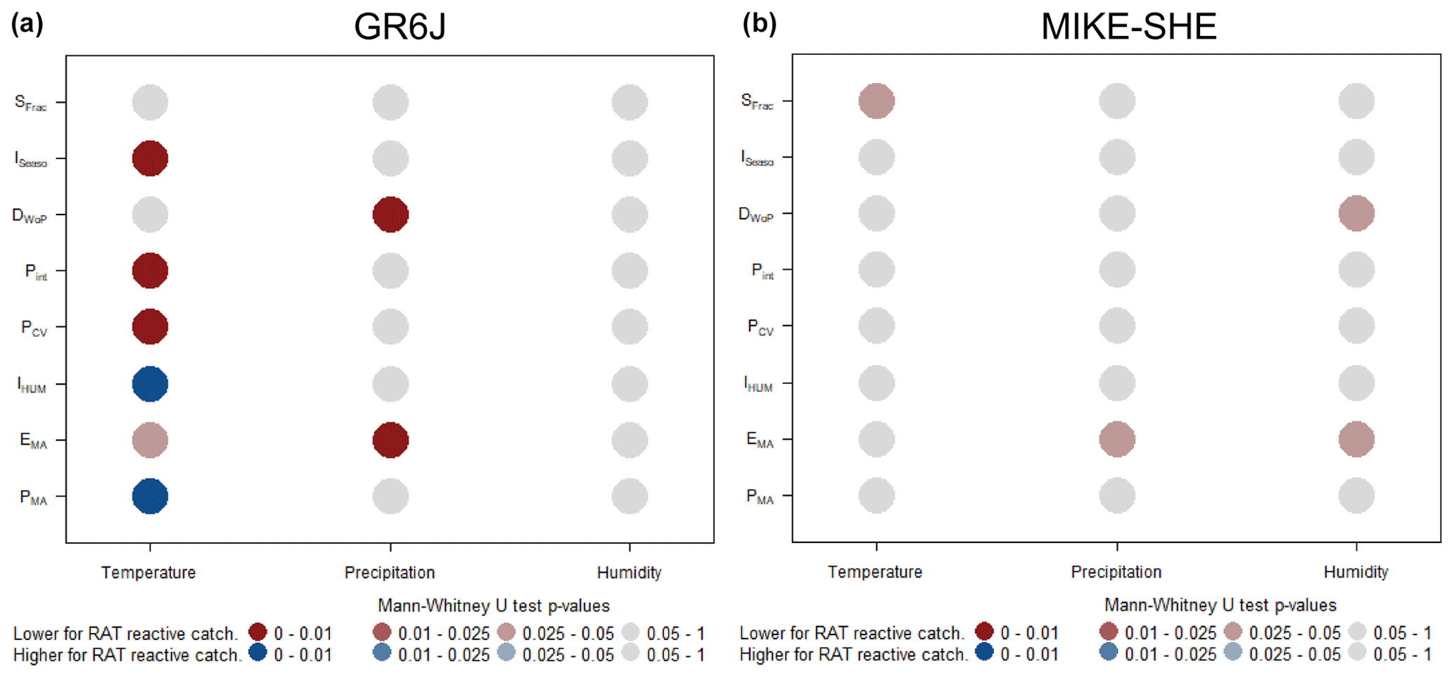
Figure 12 Results of the Mann–Whitney U test to evaluate the differences in climatic signatures in Denmark. Panel (a) represents differences between Danish catchments in which GR6J reacts and catchments in which it does not, and panel (b) represents differences between catchments in which MIKE SHE reacts to the RAT and catchments in which it does not. The number of catchments in each subset can be found in Fig. 11. Blue (red) squares mean that the signature is significantly higher (lower) for reactive catchments. P_MA: mean annual precipitation, E_MA: mean annual evaporation, I_HUM: humidity index, P_CV: precipitation variability, P_int: precipitation intensity index, D_WoP: ratio of days without precipitation, I_Seaso: seasonality index and S_Frac: snow fraction.

In the case of MIKE SHE, very few differences seem to exist between the catchments in which the model reacts and the catchments in which it does not (Fig. 12). If temperature is the predictor, the catchments in which the model reacts are less snowy than the average. If precipitation or humidity index is the predictor, the reactive catchments are characterized by less potential evaporation and fewer days without rainfall (for humidity index as the predictor).

Regarding flow signatures (Fig. 13), GR6J shows different results in Denmark than in the entire catchment set (Fig. 7). Reactive catchments are characterized by high baseflow and slow responses (precipitation and humidity index as the predictors). The reason may be the same as for the whole dataset (Sect. 3.2).

Figure 13 Results of the Mann–Whitney U test to evaluate differences in flow signatures in Denmark. Panel (a) represents differences between Danish catchments in which GR6J reacts and catchments in which it does not, and panel (b) represents differences between catchments in which MIKE SHE reacts to the RAT and catchments in which it does not. The number of catchments in each subset can be found in Fig. 11. Blue (red) squares mean that the signature is significantly higher (lower) for reactive catchments. Q_mean: annual mean flow, Q_[0.01−99]: flow percentiles, Q_{[hf−lf]freq}: frequency of high- and low-flow events, Q_[hf−lf]dur: duration of high- and low-flow events, I_BF: baseflow index, S_FDC: slope of the flow duration curve, $Q_{[\mathrm{C}-\mathrm{L}-\mathrm{H}]\mathrm{V}}$: total low- to high-flow variability, Q_AC: flow 1 d autocorrelation and R_R: runoff ratio.

MIKE SHE shows some similarities to GR6J regarding the characteristics of the catchments in which it reacts to the RAT when the humidity index is taken as a predictor. The reactive catchments for MIKE SHE have a higher baseflow and a slower response than the average, similarly to GR6J. Surprisingly, this is not the case when precipitation is taken as a predictor, even if the reactive catchments are almost the same.

To summarize, the GR6J model shows robustness issues for the same type of catchment in Denmark as for the whole dataset. Comparing the models, fewer catchments react for MIKE SHE than for GR6J, even if some similarities exist between the catchments that react for the two models. It is, however, difficult to characterize these catchments for the MIKE SHE model due to their low number.

4.3 Summary and discussion of the model comparison

The RAT was used to compare the robustness of GR6J and S-HYPE in Sweden and GR6J and MIKE SHE in Denmark. Overall, the number of RAT-reactive catchments (Table 4) can be seen as a rough indicator of model robustness. The results show that GR6J is slightly more robust than S-HYPE in Sweden and that MIKE SHE is slightly more robust than GR6J in Denmark. However, these numbers should not be the only indicator of model robustness since their use does not facilitate our understanding of the robustness issues.

Table 4 Number of reactive catchments for each country and model and proportion in terms of the total number of catchments (N=352: 163, 43 and 146 for Sweden, Denmark and France, respectively).

To improve this understanding, characterization of the reactive catchments shows that MIKE SHE and GR6J both react to the RAT in catchments with high baseflow, which indicates that both models have difficulties in representing long-term groundwater evolution. This seems to be a critical issue for model robustness (and thus a possible priority topic for model improvement). The characterization also shows that GR6J and S-HYPE robustness is sensitive to potential evaporation. The calculation of potential evaporation for the models may also lead to robustness issues (this was also shown by, for example, Birhanu et al., 2018). To confirm this, we tested GR6J in the French catchments using the Penman–Monteith evaporation formula (which is less dependent on temperature). This test showed that, even if the number of reactive catchments decreases when temperature is the indicator, the number of reactive catchments increases when both precipitation and humidity index are the indicators, which shows that the choice of formula is not straightforward. This is probably due to the fact that the model is not built to take this into account and that calibration may have led to distorted values of parameters.

The choice made in this paper was essentially to try to explain the model robustness flaws on the basis of issues in the model structure (e.g. the water balance function of GR6J). However, the model comparison cannot be fully understood without taking into account the difference in the calibration process. In particular, Fig. 10 shows that catchments in which S-HYPE presents robustness issues are difficult to characterize. The manual calibration with local tuning may provide a potential explanation for this. In addition, it is important to note that S-HYPE was only calibrated on a sub-period (between 1999 and 2008), which may consequently affect the robustness of the model compared to GR6J, which was calibrated over the whole period. The objective function is also an important factor in explaining the results of the RAT. Indeed, GR6J and MIKE SHE were calibrated by taking into account the water balance bias (within the KGE for GR6J and as one of the objective functions for MIKE SHE). S-HYPE was only calibrated with regard to the NSE with a focus on flood forecasting, which does not include an explicit water balance component. Because of the way the RAT is designed (using the water balance bias as a metric), this has probably also affected the results of the S-HYPE model. Consequently, although this is most likely not the only factor, calibration choices may explain why S-HYPE appears slightly less robust than GR6J and why the reactive catchments are so difficult to characterize. These differences in terms of calibration processes are difficult to overcome since the models have different structures that require different calibration processes. It is, then, difficult to avoid here since one of the aims of the paper is to compare models with different modelling philosophies.

4.4 While all that glitters is not gold, not all that is dull is worthless

The meaning of a reaction to the RAT needs to be discussed. By itself, it only indicates that the annual model bias is correlated with a given climate indicator. Although it is a bad omen regarding the capacity of extrapolation of the model, its interpretation is not straightforward: it is a “yes-or-no” test that requires interpretation. The slope of the relationship between bias and indicator may also be interesting to examine, since a low slope is certainly not as problematic as a high one.

If a model reacts to the RAT, it could also be for “good” reasons, i.e. because of a time-dependent bias in the forcing data or a drift in the measured streamflow. Even a robust model will be affected by a trend in input data, giving the impression that the hydrological model lacks robustness. Such an erroneous conclusion could also be due to widespread changes in land use, construction of an unaccounted-for storage reservoir or evolution of water uses.

If a model does not react to the RAT, this does not mean that it has no robustness issue at all; indeed, the RAT is designed to only give an initial diagnosis of model health. However, the large-sample analysis carried out in this paper gave an overall idea of the robustness of the models by using a large dataset. It allowed us to find patterns in the model robustness issues that served as a diagnosis to improve these issues in the future without having to deploy a complex experimental set-up.

In the same vein, it is interesting to evaluate how much the results of the RAT are influenced by the performance of the models. Indeed, the performance can have two possible effects: if the performance is too low, the model may react to the RAT because it does not represent the hydrological processes in the catchments correctly, but if the performance is very high, it may be that the model is over-adapted to the calibration period and will react to the RAT. However, if the model does not show high performance over the observed period, it is likely that the performance in a future climate will remain low, leading to high uncertainties in flow projections. It is therefore important to add a performance check to the RAT. For example, Gelfan et al. (2020) proposed such a method in which the model is not seen as robust if it remains under a certain performance threshold. In the case of our study, the performances are good overall. All three models have a KGE value higher than 0.7 in 329 catchments of the 352.

Although we are confident that the RAT is useful, it is not a universal panacea for hydrological models.

5 Conclusions

5.1 Synthesis

This paper presented a large-sample analysis of the robustness of three models to a changing climate. The RAT allowed us to evaluate the robustness of the three different models without controlling their calibration process, and the analysis of the hydrological signatures of the catchments that react to the RAT suggested some potential issues specific to each model. Our objective was not to compare models, as we have shown that they all suffered from a lack of robustness for safe application in a changing climate context, but to identify the hydrological features that could be the cause of this lack of robustness. Overall, the models reacted to the RAT in a significant number of catchments (between 33 % and 42 %, depending on the model and the datasets), and this indicates that much work is needed to make models more robust in the context of climate change.

5.2 How generic are our results?

The issue of genericity is central to science. With the application of the RAT in three models, in three countries and in a total of 352 catchments, the work presented in this paper presents a significant improvement over what had initially been done in the work describing the method (Nicolle et al., 2021). Because models are used more than ever to predict the impact of a changing climate, we believe more than ever in the need to test them more thoroughly and in the need to challenge their extrapolation capacity. Because the RAT is so simple to apply and because it can be applied to models requiring calibration that run in seconds and to models that need hours to produce a single run, we consider it a useful investment for modellers and model users, one that is likely to “increase their confidence” in their results, as de Marsily et al. (1992) recommend.

Of course, we keep in mind the advice that the late Vit Klemeš (personal communication) gave one of us. Asked how he looked back at the impact of his famous paper discussing the different options of split-sample testing (Klemeš, 1986), he answered that he had in fact always been sceptical about the capacity of hydrologists to validate their models rigorously: he said he knew in advance that the tests he had suggested would be “avoided under whatever excuses available because modelers, especially those who want to “market” their products, know only too well that they would not pass it”, adding that he had “no illusions in this regard” when he wrote his paper. We do not have any illusions either, and we do not wish to fight against windmills. We modestly think it is part of our scientific duty to keep expressing our concerns on this topic.

5.3 Perspectives

Our analysis pointed out flaws in the models in terms of robustness to a changing climate.

First, the climatic and flow signatures used in the paper do not seem to be sufficient to explain the robustness issues of the models (especially in the case of S-HYPE). In Sweden and Denmark, more snow signatures may help to refine the analysis regarding snow processes and to better understand potential issues in the model snow modules. S-HYPE may also be more sensitive to land use or soil cover since the model parameters are regionalized by HRUs (soil and land use combination). This analysis would be useful for pointing out any region or parameter in which robustness issues exist. The evolution of land use in time may also be interesting to examine, since it is also an indicator of changing climate and can induce some errors in models that are parameterized by HRUs like S-HYPE.

The analysis also highlighted some issues that are due to potential evaporation calculation. It would thus be interesting to test several formulas for the calculation of potential evaporation so as to check whether it is possible to optimize model robustness. Birhanu et al. (2018) tested the robustness of different formulas and concluded that the simplest of them do not necessarily decrease the robustness. However, these conclusions were made using an SST, and it may be interesting to test them using the RAT. We ran such a test in the French catchments using the Penman–Monteith equation and GR6J (see File S5). The test yielded conflating results, which are difficult to interpret (fewer reactive catchments when temperature is the indicator but more catchments when precipitation is the indicator).

More systematic tests are needed to better understand the influence of the calibration set-up. The RAT could, for example, be used to evaluate the effect of objective functions by using several types of criteria and flow transformations. It could also be interesting to test the influence of the period used for calibration and how period selection can be optimized to better satisfy the RAT. In the same vein, most systematic evaluations can be made in combination with progressive changes in model structure to test the robustness issues attributed to model structure and to optimize model robustness.