Technical note: A low-cost approach to monitoring relative streamflow dynamics in small headwater streams using time lapse imagery and a deep learning model

Despite their ubiquity and importance as freshwater habitat, small headwater streams are under-monitored by existing stream gage networks. To address this gap, we describe a low-cost, non-contact, and low-effort method that enables organizations to monitor relative streamflow dynamics in small headwater streams. The method uses a camera to capture repeat images of the stream from a fixed position. A person then annotates pairs of images, in each case indicating which image has more apparent streamflow or indicating equal flow if no difference is discernible. A deep learning modeling framework called streamflow rank estimation (SRE) is then trained on the annotated image pairs and applied to rank all images from highest to lowest apparent streamflow. From this result a relative hydrograph can be derived. We found that our modeled relative hydrograph dynamics matched the observed hydrograph dynamics well for 11 cameras at 8 streamflow sites in western Massachusetts. Higher performance was observed during the annotation period (median Kendall's Tau rank correlation of 0.75, with a range of 0.6–0.83) than after it (median Kendall's Tau of 0.59, with range 0.34–0.74). We found that annotation performance was generally consistent across the 11 camera sites and 2 individual annotators and was positively correlated with streamflow variability at a site. A scaling simulation determined that model performance improvements were limited after 1000 annotation pairs. Our model's estimates of relative flow, while not equivalent to absolute flow, may still be useful for many applications, such as ecological modeling and calculating event-based hydrological statistics (e.g., the number of out-of-bank floods). We anticipate that this method will be a valuable tool to extend existing stream monitoring networks and provide new insights on dynamic headwater systems.

1 Introduction

Small headwater streams make up 50 %–70 % of stream network length (Benda et al., 2004; McManamay and DeRolph, 2019) and are fundamental units of riverine networks. Streamflow dynamics in these streams are crucial controls on aquatic ecosystem function (Carlisle et al., 2017; Colvin et al., 2019; Hitt et al., 2022), thermal changes, and the routing of sediment and contaminants. Headwater streamflow dynamics are uniquely complex for the following reasons: (1) a majority of small (second-order or less) stream channels dry out seasonally or during drought events (Jaeger et al., 2021; Messager et al., 2021); (2) along-channel changes can be abrupt due to geologic controls and focused groundwater inputs (Briggs et al., 2018); and (3) due to small catchment size, these streams are particularly susceptible to drastic hydrologic alterations, both anthropogenic (damming, impervious surface runoff) and natural (ice or beaver damming, wildfire effects, geomorphic changes).

Despite their importance and vulnerability, headwater and non-perennial streams are underrepresented by streamflow monitoring networks in the United States (Deweber et al., 2014; Seybold et al., 2023) and across the world (Krabbenhoft et al., 2022). Three primary limitations lead to a sparse headwater monitoring network. First, monitoring and maintaining traditional stage-discharge gage records (Turnipseed and Sauer, 2010) at a high quality requires expertise and training that limits the number of organizations able to collect the records. Second, velocity measurements in small, shallow, and slow-moving streams are difficult to collect and have high uncertainty, making the percentage error in streamflow discharge much higher in small streams than large streams (Horner et al., 2018; King et al., 2022; Levin et al., 2023; McMillan et al., 2012). Third, in-stream instruments to measure stage in headwater streams are frequently lost or damaged due to shifting streambeds, very high local velocities, and beaver or other animal activity. Even disregarding the challenges in collecting the data, where streams are non-perennial or form disconnected pools, traditional pressure-transducer-based stage measurements provide incomplete information regarding (dis)connectedness of the stream channel, making these records inadequate for certain uses in ecohydrological modeling (Steward et al., 2012).

Streamflow monitoring using imagery is an attractive alternative to in-stream instruments and has grown in popularity as camera technology has improved. Collecting imagery is appealing because it requires very little training or specialized equipment. However, analyzing a large volume of imagery can be a challenge; a range of approaches have been introduced to date. Initially, manual interpretation (Schoener, 2018) or rules-based image processing techniques (Chapman et al., 2022; Gilmore et al., 2013; Leduc et al., 2018; Noto et al., 2022) were used to automate the reading of a staff gage placed in the channel. While effective and low-cost, these staff-plate-based approaches still require the installation of in-channel infrastructure that may not be permitted in protected lands or can be damaged by high flows. Additionally, stage monitoring is restricted to the location of the staff plate; therefore, any debris on the staff plate or view blockage due to snow or vegetation will result in missed readings. Computer-vision-based approaches that avoid the use of an in-channel staff plate have been introduced but generally require the manual identification of a specific region of interest in the image (Keys et al., 2016), image orthorectification using ground control points, and detailed high-resolution 3D models of riverbed and bank geometry to estimate changes in stage (Eltner et al., 2018).

Advances in deep learning approaches for imagery analysis have created new opportunities for environmental monitoring. For example, several recent studies have applied deep learning to image-based stream stage monitoring to eliminate the need for fixed in-stream staff plates. Many of these papers use established image segmentation algorithms (i.e., convolutional neural networks) to classify parts of the image as “water” or “not-water” (Eltner et al., 2021; Liu and Huang, 2024; Vandaele et al., 2021). Using a reference point on the image and knowledge of the interface location, the stream level is tracked over time. While effective, these approaches are sensitive to channel rearrangement or view blockage at the water–not-water interface. They also still require some manual judgment about the location of interest in the image frame for which stage is provided and image orthorectification using ground control points.

Unlike other deep learning approaches for streamflow estimation, streamflow rank estimation (SRE) was developed to minimize the need for external monitoring data to train a model (Gupta et al., 2022). The approach aims to estimate streamflow dynamics without the need for traditional discharge observations, an in-channel staff plate, designating a region of interest, or imagery orthorectification. SRE uses a learning-to-rank framework that is trained using many pairs of stream images, with discharge in the images of each pair visually compared, removing the need for stream discharge training data. We refer to the person-generated pairwise ranks as “annotations”. The model is trained using the annotations to sort images from high apparent streamflow to low apparent streamflow by fine-tuning a convolutional neural network (a ResNet-18, He et al., 2015; architecture pretrained on ImageNet, Deng et al., 2009) and using a learning-to-rank approach utilizing the RankNet loss function (Burges et al., 2005). The rank of each image can be used to create a streamflow percentile which is correlated with the streamflow discharge and can be interpreted as a dimensionless hydrograph. While the absolute streamflow could be estimated from the streamflow percentile using an assumed streamflow discharge distribution, for unmonitored catchments this distribution would need to be estimated independently of the SRE model and would be a significant source of uncertainty in absolute streamflow estimates (Gupta et al., 2022). As a trade-off for low-effort model training and minimal external information requirements, the rank-based streamflow percentile estimate is the primary output produced by the SRE model.

To date, the SRE model has been tested at a limited number of sites with simulated annotations derived from known streamflow discharge time series, but not with annotations created by people. With simulated annotations, SRE characterized streamflow percentile dynamics with a Kendall rank correlation greater than 0.7 in five of six stream locations (Gupta et al., 2022). The number of annotations (n = 500, 1000, 2500, 10 000) and annotators' ranking ability (could discern 0 %, 10 %, 20 %, or 50 % discharge difference) both strongly influenced the model's ranking performance. This promising early work motivated us to further evaluate the real-world performance of the model by using person-generated annotations and expanding the number of stream sites at which we assessed model performance. With a better understanding of the factors influencing model performance, we plan to apply SRE to currently unmonitored headwater catchments.

This paper describes a methodology for monitoring relative streamflow dynamics in small headwater streams using time lapse imagery coupled with a deep learning model trained using person-generated annotation. We evaluate the real-world performance of this monitoring system and answer the following questions:

• 1.

  How accurate are people at ranking images by streamflow?

• 2.

  How accurate are the image-derived relative hydrographs developed using person-generated annotations?

• 3.

  Which factors influence ranking model accuracy and can indicate which unmonitored catchments would be suitable for low-cost camera monitoring?

• 4.

  How many person-generated annotations are required to achieve stable ranking model performance?

2 Methods

2.1 Data collection

To collect time lapse imagery from low-cost cameras, this project developed a web platform titled the Flow Photo Explorer (https://www.usgs.gov/apps/ecosheds/fpe/, last access: 13 November 2025). Since its inception in October 2021, the Flow Photo Explorer (FPE) platform has accepted imagery submissions from an array of organizations with a common motivation of enhancing and expanding stream monitoring networks. While guidelines are provided on the web page, there are few restrictions on how cameras are configured and what views they capture. The only requirement is that the imagery format uploaded to the FPE platform is formatted with EXIF metadata, which is a common imagery data format across many low-cost battery-powered game or trail cameras. We recommend a photo every 15 min, though the FPE database contains intervals from less than 5 min to once per day. The recommended camera view is looking downstream or upstream, though based on field conditions some sites may instead feature cross-stream or tangential views. We expect that the image-based monitoring approach will work best when at least some fixed objects (i.e., trees, boulders, bridge pilings, stream banks) are visible at all levels of streamflow. An example camera view with these fixed features visible is shown in Fig. 1. If a user knows a US Geological Survey (USGS) stream gage monitoring the same stream reach, they can indicate the USGS station identifier, and data are automatically pulled from the USGS National Water Information System (U.S. Geological Survey, 2024) database. Alternatively, they can upload their own streamflow observations, although they are not required. To test the methodology, we co-located 11 cameras with 8 USGS gages in western Massachusetts for which records of stream discharge are available (Fair et al., 2025). Four cameras were located at the same streamflow monitoring location to examine the effect of differing camera angles on monitoring performance. In this study we collected imagery every 15 min with Reconyx (Hyperfire 2 model) and Bushnell (Trophy and Essential models) cameras that were mounted to trees (except for one site that was affixed to a bridge) using swivel mounts and a secure metal housing.

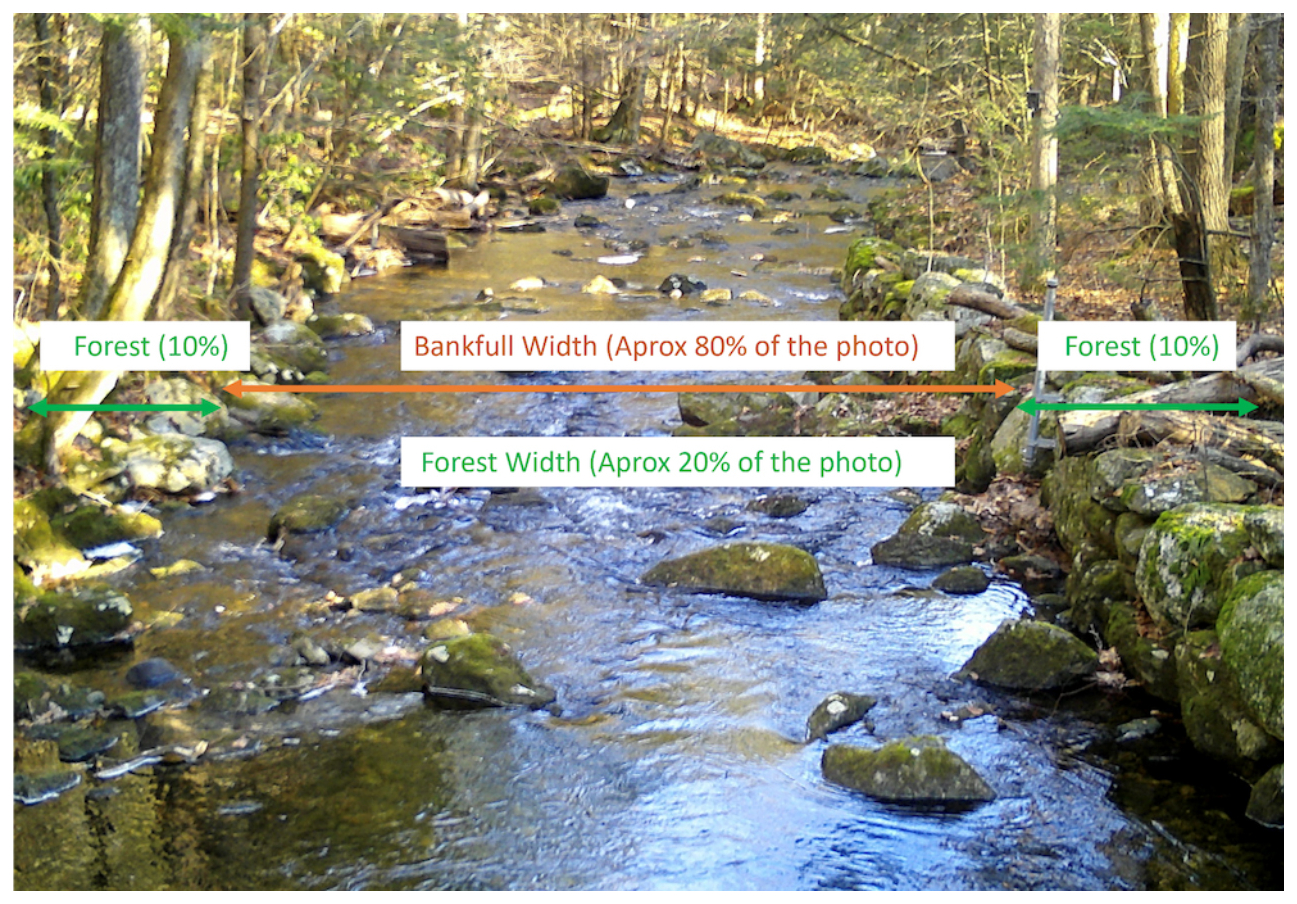
Figure 1 The recommended camera view includes stream banks and fixed objects such as trees or boulders visible at most flows. Photograph by the US Geological Survey.

For this analysis we set minimum data availability criteria to test the method at sites with sufficient data. We expected that seasonal changes in vegetation, streamflow, and snow cover would appear in the imagery. Therefore, we selected sites with stream discharge and imagery data that spanned at least 1.5 years. We implemented this criterion to ensure that the model training period spanned at least 1 full year so that all seasons were represented and so that we additionally had access to a final half year of data for testing purposes. Within this span, we allowed some data gaps, since these are common in our available set of imagery data. We required at least 180 complete days of data within the 1.5 years, which is a completeness of approximately 33 %. Table 1 contains a list of sites that met our data availability requirements. These locations are mapped in Fig. 2. In this analysis we used daytime-only imagery (from 07:00 to 19:00 local time (UTC-5)), though many sites have cameras with an infrared flash that also produce usable imagery at night.

Table 1 Summary of data collected at locations included in this analysis. Streamflow observations were originally reported in a US Geological Survey (USGS) data release (Fair et al., 2025). “Training period CV of log ₁₀(Q)” refers to the coefficient of variation of log-transformed streamflow discharge during the model training period.

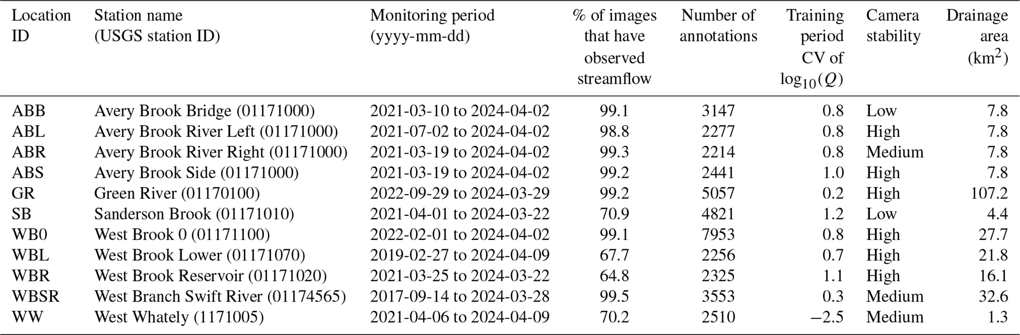
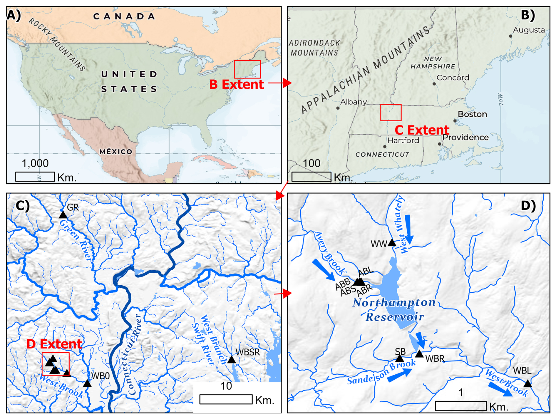
Figure 2 Map of monitoring locations in western Massachusetts, USA (Fair et al., 2025; Goodling et al., 2025). Triangles in panels (c) and (d) indicate monitoring sites and are labeled with site identifiers listed in Table 1. Arrows in panel (d) indicate streamflow direction. Water bodies shown are from the NHDPlus Version 2 (McKay et al., 2012) (c) and NHD High Resolution (Moore et al., 2019) (d) datasets.

To guide user site selection and setup, we evaluated patterns in model performance according to two key site attributes. The first is a measure of flow variability during the monitoring period. Some streams, such as those heavily influenced by groundwater discharge, can have small fluctuations in stream stage that are difficult to identify in imagery. We selected the coefficient of variation (CV) of log-transformed streamflow (log ₁₀(Q)) to quantify the general variability in the stream. The second metric is a simple qualitative assessment of how stable the camera view is over the period of record. This metric is primarily for quantifying if there were abrupt changes in the field of view of the image time series, mainly coinciding with when the camera was serviced. Cameras can also shift slightly due to vibrations or wind changing the mounting position, though these types of shifts are minor alterations compared to abrupt view changes. In this rating system, a camera stability value of “low” indicates that there was at least one camera view change of 50 % or greater (i.e., only half of the original frame was still visible). “Medium” indicates at least one camera view change between 25 % and 50 %, while “high” indicates that all view changes were below 25 %. These two attributes were selected to inform user site selection and field methods.

2.2 Data annotation

Training the neural network model to predict streamflow dynamics from imagery requires external site-specific information. Because we hope to use this method in places with no other information except for the imagery, we could not use any streamflow data in model training. Instead, we relied on people to rank pairs of images by streamflow in a process called “data annotation”. In the FPE web application, users were shown two photos from a given site side by side and asked to indicate which one had more streamflow (Fig. 3). The images selected to form a pair were selected at random. The users also indicated if the images appear “about the same” or if the image was a “bad photo” (obscured or too dark). “Don't know” was selected if the photo is bad or if other aspects of the images made them difficult to compare, such as a large difference in camera view or camera angle. Image pairs marked “don't know” were not used in model training. In this study, users were only presented with images collected during daytime (07:00–19:00; all times are given in local time). A typical user completed an annotation in 1–3 s on average; if focused, an individual could perform approximately 1000 annotations in an hour. Our dataset includes 17 unique annotators who contributed to the model training; however, only two annotators represent 93.7 % of all the annotations, and we focus on these two in our discussion of annotator performance. Both of these annotators were student interns (one ecology graduate student, one environmental science undergraduate student). The student interns were associated with the project but had no specialized training or experience in streamflow monitoring.

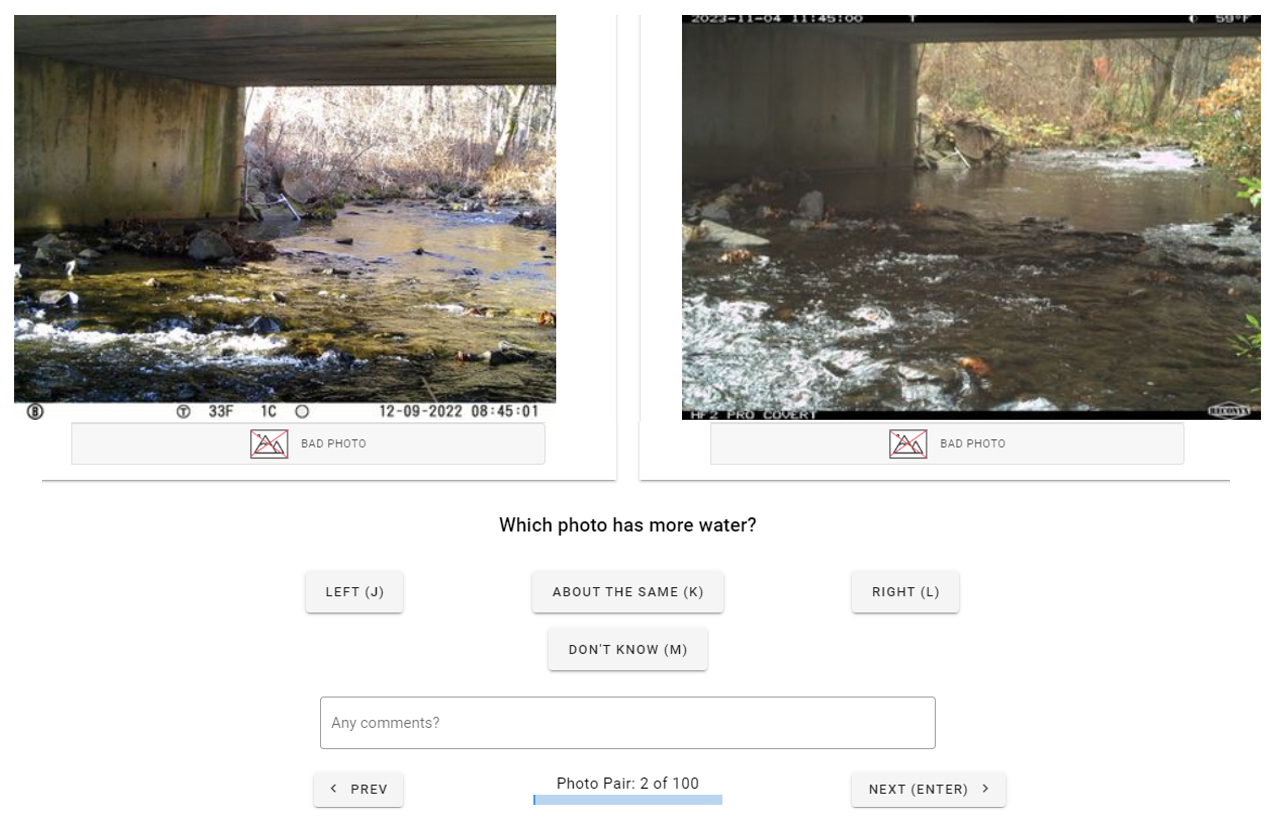
Figure 3 The web-based annotation interface from the Flow Photo Explorer used in this study to develop training datasets for the ranking model.

The process of annotation was not error-free; the judgments made by individual annotators could sometimes be incorrect. This could be through simple errors in transcription (i.e., clicking the incorrect button) or because the imagery pairs were difficult to compare because of lighting, vegetation, or seasonal differences. These errors, if significant, could provide spurious information to the deep learning model. We therefore quantified the performance of our annotation dataset using the known true flow-based ranks from the co-located USGS gage data. Our primary metric was classification accuracy for the selection of the “left” or “right” image with higher streamflow in the image pair:

$$\begin{array}{}\text{(1)}& \mathrm{\text{Classification}}\mathit{\%}\text{accuracy}={\displaystyle \frac{\text{TL}+\text{TR}}{\text{TL}+\text{FL}+\text{TR}+\text{FR}}}\times \mathrm{100},\end{array}$$

where TL and TR refer to true-left and true-right selections, and FL and FR refer to false-left and false-right selections. We observed that the difficulty of the selection increases, and therefore the classification accuracy decreases, if the two photos had similar streamflow. To fully describe annotation performance, we provide our metrics as functions of the relative flow difference between the images. The relative flow difference (Δ_rel) between a pair of photos shown to an annotator was calculated as

$$\begin{array}{}\text{(2)}& {\mathrm{\Delta }}_{\mathrm{rel}}={\displaystyle \frac{\left|Q_{\mathrm{1}}-Q_{\mathrm{2}}\right|}{\frac{\mathrm{1}}{\mathrm{2}}\left(Q_{\mathrm{1}}+Q_{\mathrm{2}}\right)}},\end{array}$$

where Q₁ and Q₂ represent streamflow values for the two images. For positive values inclusive of zero, the value Δ_rel is bounded to be between 0 and 2. A Δ_rel value near zero indicates close agreement between Q₁ and Q₂, whereas a Δ_rel value of 2 could indicate that one of the two values is approaching zero or infinity. We compute the overall classification accuracy within binned increments of 0.1 Δ_rel; the unweighted binned performance is used to develop a function describing the relationship between Δ_rel and classification accuracy.

2.3 Modeling methodology

Annotated images were ranked into an ordered sequence using the previously developed SRE neural network model (Gupta et al., 2022). An independent model was trained for each site. The SRE neural network model takes an image as input, which includes three channels (RGB), and generates a dimensionless, continuous valued score representing relative streamflow as output. The score is derived by applying a sequence of mathematical operations to the input image, including spatial convolutions, which help the model extract relevant features from the image. During training, the model is given batches of paired images ranked by annotators based on relative streamflow. Two neural networks with shared model weights sequentially predict dimensionless scores for the two images. The pair of scores is used to compute a probabilistic ranking loss (Burges et al., 2005) that is minimized when the model assigns a higher score to the image that the annotator ranks as having higher flow or assigns the same score to both images if the annotator ranks them as having the same flow. This architecture is sometimes called a “twin neural network”. Images are pre-processed by resizing, center-cropping to exclude metadata bands, and normalizing. While training, data augmentations such as random crops, horizontal flips, rotations, and color jitter are applied to improve model robustness and generalization and reduce overfitting (Shorten and Khoshgoftaar, 2019). Additional detail on model development and image pre-processing is available in the Supplement. After training, the model is used to generate score predictions for all images from a site, which are then standardized into z scores by subtracting the mean and dividing by the standard deviation.

The imagery data were divided into training, testing, and validation splits to enable robust model evaluation. Unlike many machine learning applications, the model learns from image pairs and not individual images; therefore, these splits are a bit more complex to develop. When reporting model performance, we identify images that comprised pairs used for training (“train”, representing 80 % of annotations) or validation (“val”, representing 20 % of annotations). Images that were not part of any annotation pair provided to the model are used for “test”. We further divided this into “test-in”, which is coincident with the time frame of annotation, and “test-out” (when available) for the period following the period with annotations. “All-in” is the combined set of images, regardless of if they are part of an annotation pair, during the annotation period. “All” is the performance for all images. We consider “test-in” to represent a retrospective model performance, while “test-out” represents the expected performance of a deployed operational model on new imagery.

The sites in this study were co-located with traditional USGS streamflow gages, which enables us to evaluate model performance relative to these instruments. Our model performance metric is Kendall's Tau, a nonparametric rank-based correlation coefficient (Kendall, 1938). We selected this metric because it is insensitive to monotonic transformations such as log-transformation and percentile calculations, making it appropriate to compare values on different scales and with different distributions. As a metric it is strict regarding timing; short-lived peaks, if slightly mistimed, will result in low Kendall's Tau. Because it is based on ranks, it is insensitive to the magnitude difference between two values. As a result, low-flow observations, which are more common, have a greater influence on the resulting Kendall's Tau than short-lived high-flow observations.

To provide a preliminary understanding of the factors influencing model performance we present pairwise relationships between annotation accuracy, streamflow variability, camera stability, and model performance. For comparisons among the numeric values we present the Pearson correlation coefficient and two-sided p value calculated with the cor.test function in R version 4.3.2 (R Core Team, 2021). For comparisons between numeric values and the categorical camera stability metric, we present the results of the nonparametric Kruskal–Wallis test to evaluate if the distribution varies among the categories (Kruskal and Wallis, 1952). If significant, we perform Dunne's post hoc pairwise multiple comparison test to identify which categories have statistically different distributions (Dunn, 1964). The Kruskal–Wallis and Dunne tests are computed with the rstatix R package (Kassambara, 2023).

2.4 Sensitivity analysis

We performed a sensitivity analysis to understand how many person-generated annotations are required to achieve acceptable performance. In this case, the target performance level was that achieved by training the model with all available image pair annotations for a given site. We created nested subsets of the annotations, beginning with increments of 100 up to 500, then using larger increments of 250 up to 1500, and finally using increments of 500 up to 3000, with additional subsets at 4000 and the maximum number of available annotations. Smaller increments were used at the lower end of the annotation range to capture the more substantial improvements in model performance that are typically observed with initial increases in training data. Each subset was a strict superset of the previous one, meaning that each larger subset contained all the pairs from the smaller subsets plus additional pairs. This allowed us to assess how increasing the volume of training data impacts model performance and to identify the point where performance plateaus, avoiding unnecessary annotation efforts that may not significantly improve performance. The sensitivity analysis reported that the Kendall Tau model performance metric is for the “test-in” data split for daytime images (07:00–19:00 local time).

To ensure the robustness of our findings, the analysis was repeated five times. For each repetition, we randomly permuted the order of the annotations before generating the nested subsets, thereby mitigating any potential variance that could arise from the specific sequence of training samples.

3 Results

3.1 Annotation results

Annotation performance in our dataset was high (average 92.2 % accuracy) and was generally consistent across sites and annotators. Accuracy was well described by an increasing function of the relative flow difference (global fourth-order polynomial, R² = 0.89; Fig. 4, red lines). At all sites, annotation accuracy neared 100 % accuracy above a relative flow difference of 1 (which occurs when one image has 3 times as much streamflow as the other). As the relative flow difference neared 0, classification accuracy approached 50 %, which is equivalent to guessing between the photos. Similar curves are observed for the two primary annotators (represented by symbols in Fig. 4). To characterize the overall accuracy of the annotation at a site, the percent accuracy of all annotations regardless of relative flow difference is reported in each panel of Fig. 4. The site with the lowest overall annotation performance – West Whately, with an 84 % overall accuracy – had the lowest streamflow coefficient of variation a “medium” level of camera stability (Table 1).

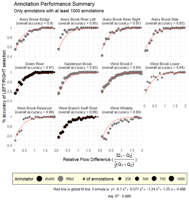
Figure 4 Annotation accuracy for each site as a function of the relative difference in streamflow between the two images shown to the annotator. Percent accuracy was computed for annotations in binned intervals of 0.1 relative flow difference. Two annotators (represented with symbols and named with five-digit alphanumeric identifier) performed annotations across the 11 camera sites. The red line is a fourth-order polynomial fit across all 11 camera sites, with equation and fit statistics shown at the bottom of the figure.

3.2 Modeling results

Predictions from models trained on person-generated annotations were found to represent both individual storm events and inter-annual hydrologic changes with a satisfactory degree of fidelity, with “test-in” Kendall's Tau values ranging from 0.60 to 0.83 (Fig. 5). We separately report statistics for the data splits “test-in”, “test-out”, “all-in”, and “all”. Most models have a slight decrease in performance (approximately 0.02) when comparing the training to test-in results. This decrease is a measure of overfit to the data. Green River has the greatest decrease (0.08, or 10 %). A review of the annotations for this site shows a low density in annotations at the end of the training period that could account for this difference. Where available, the test-out performance is lower than test-in performance (mean decrease is 0.20), suggesting a decreased ability to generalize to new flow conditions or camera views.

Within our camera monitoring dataset, we have several co-located cameras that were independently annotated and trained (lighter color bars in Fig. 5). Four co-located cameras exhibited similar test-in performance, although a downstream-facing view had slightly lower performance than the other three. For the test-out period, two sites (Avery Brook River Left and Avery Brook Side) have much better performance than the other two. These sites have “high” camera stability and greater annotation accuracy than the other two sites. The streamflow has a similar (but not identical) coefficient of variation due to the differing monitoring time frames among the cameras.

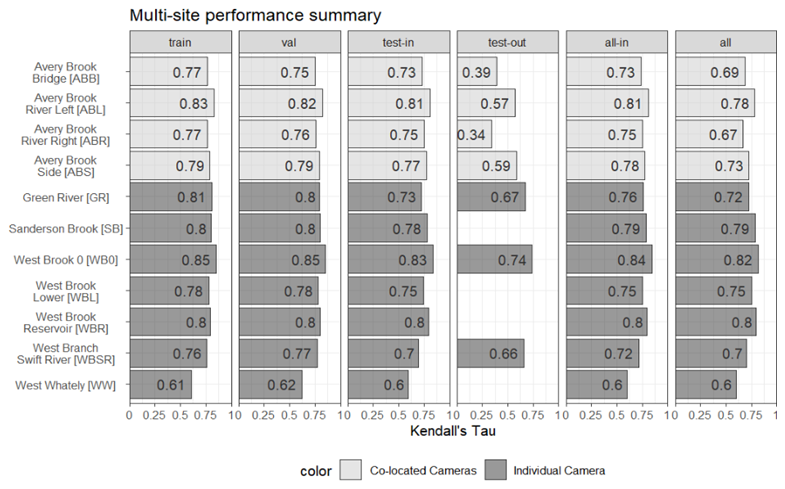
Figure 5 Summary of model performance, as defined by Kendall's Tau correlation, between observed and estimated streamflow percentile. Results are presented for 11 sites, 4 of which are co-located. Site abbreviations shown in brackets. Results are presented for six different sets of the data. The set “test-in” represents unseen images coincident with the training period. The set “test-out”, which is not available at all locations, represents unseen images following the training period.

Model prediction time series show a clear correspondence with observed streamflow time series, especially when both datasets are displayed as rank percentile units (Fig. 6; the Supplement). Major hydrologic events such as a drought that occurred in this area from June–September of 2022 and a prolonged wet period in July–August of 2023 are visible in the estimates derived solely from the imagery model. The duration and magnitude of major hydrologic events match well between observed streamflow and model predictions. Short-lived peaks from individual storm events are also well characterized by their timing and general magnitude.

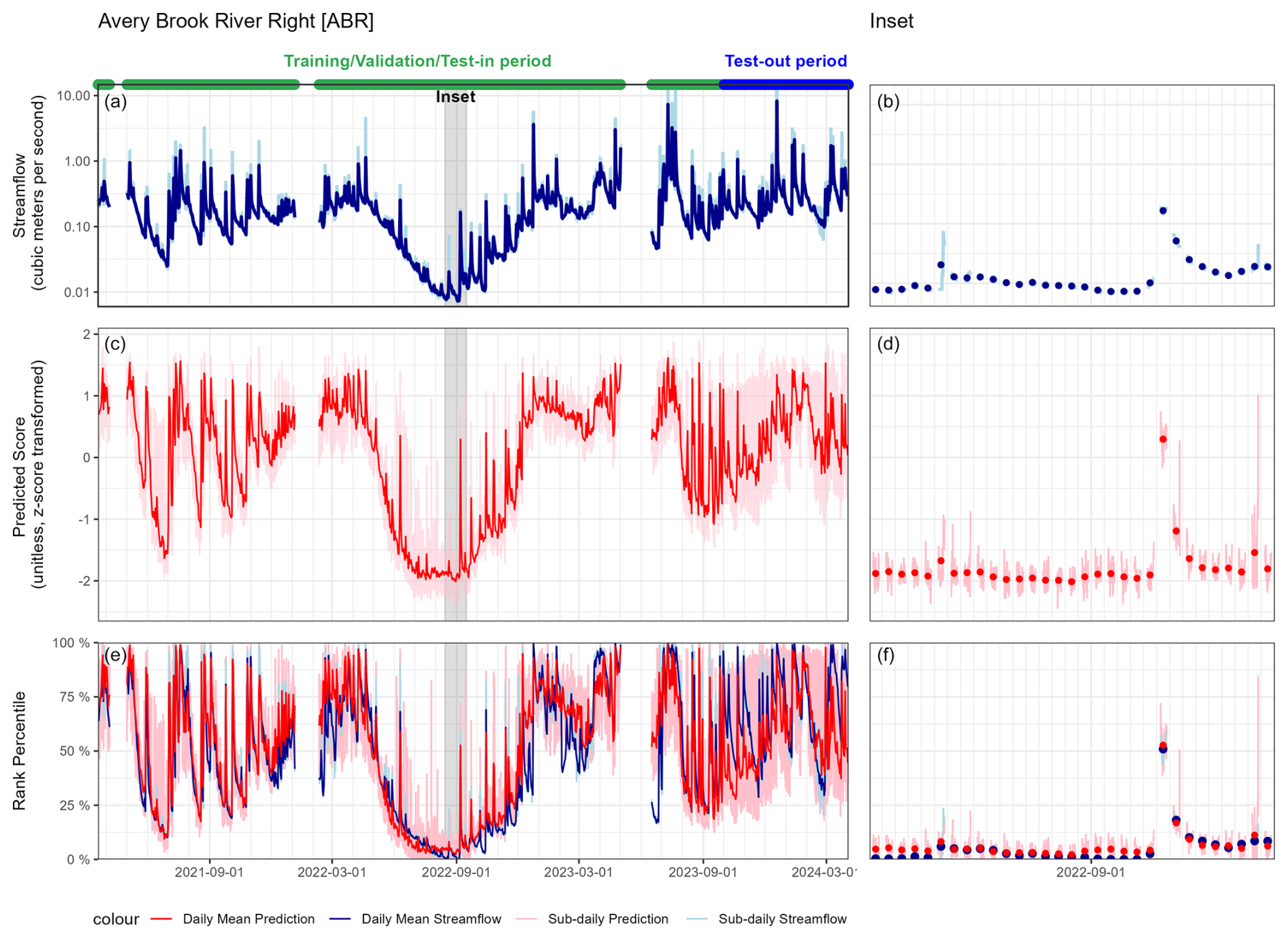
Figure 6 Time series prediction at a single site representing intermediate model performance. Panels (a) and (b) show the streamflow, panels (c) and (d) show the predicted model score, and panels (e) and (f) show both when transformed to rank percentile. The left column indicates the full period of record; the right column is an inset. In the inset plots, daily means are plotted as dots, and the 15 min interval predictions are plotted with lines. Prediction time series for all sites are shown in the Supplement.

Model performance of the “test-in” set, annotation performance, flow variability, and camera stability were found to be highly interrelated (Fig. 7). Positive correlations were observed between flow variability and annotation accuracy (panel a), flow variability and model performance (panel c), and annotation accuracy and model performance (panel d). West Whately is an outlier to some extent; we report Pearson's correlation coefficients and p values with and without this camera site. The relationship between annotation accuracy and model performance (panel d) has the highest correlation and is least affected by the outlier presence. Camera stability, a categorical variable, was weakly related to annotation accuracy (panel b). The Kruskal–Wallis test indicates that the annotation performance is non-identical across the three stability classes at the 0.05 significance level. The post hoc Dunn pairwise multiple comparison test shows the only significant difference is between the “high” stability and “medium” stability classes. The Kruskal–Wallis test indicates there is no significant difference in Kendall's Tau among the stability classes (panel e). Among the four cameras located on the same stream reach (shown with lighter shading), the highest performance in annotation accuracy and test-out Kendall's Tau was observed for Avery Brook River Left, which had a highly stable camera.

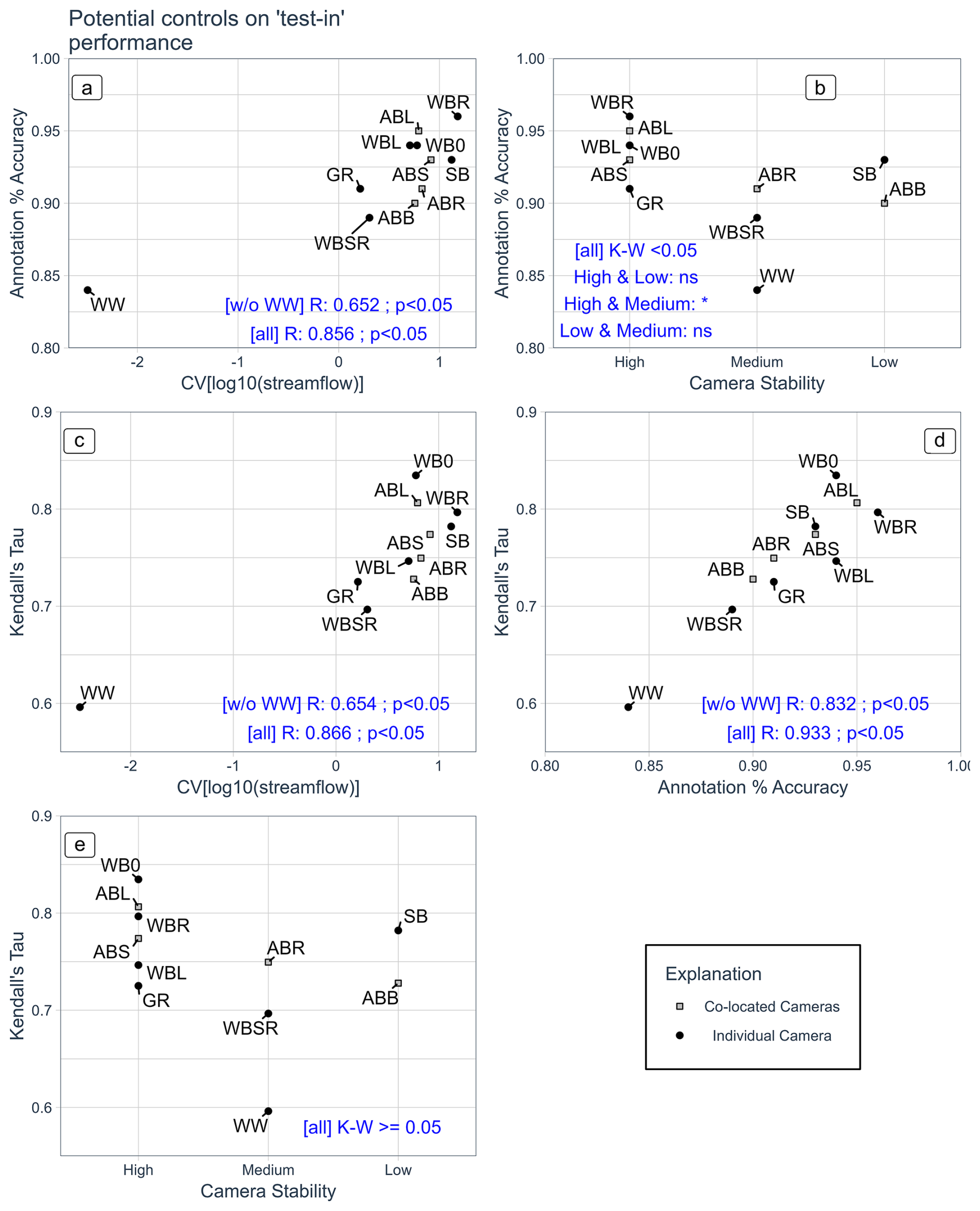
Figure 7 Relationships between flow variability and annotation accuracy (a), camera stability and annotation accuracy (b), flow variability and model performance (c), annotation accuracy and model performance (d), and model performance and camera stability category (e). Flow variability is quantified with the coefficient of variation of log-transformed streamflow. Model performance is the “test-in” split. Point labels refer to the site numbers listed in Table 1. The four co-located cameras are indicated with light-gray square symbols. Panels (a), (c), and (d) have text indicating Pearson's correlation coefficient and significance at the p < 0.05 level; values are provided without the West Whately site (“w/o WW”) and for all sites (“all”). Panels (b) and (e) have text with the Kruskal–Wallis significance test at the p < 0.05 level. Where significant, the post hoc Dunn pairwise multiple comparison test is performed. An asterisk indicates significance at the p < 0.05 level, while “ns” indicates not significant at that level.

3.3 Sensitivity analysis

The sensitivity analysis we employed allowed us to examine the relationship between number of annotations and model performance. For most sites, “test-in” model performance improves significantly from 100 annotations to 500 annotations, as the models learn more relevant features for inferring relative streamflow (Fig. 8). Generally, the spread of individual iterations (n = 5) was small relative to the performance improvement associated with increasing annotations. The model performance plateaus around 1000 annotations for most sites. Beyond this point, additional annotations offer minimal gains, suggesting that the model is not extracting further useful information from the additional annotations.

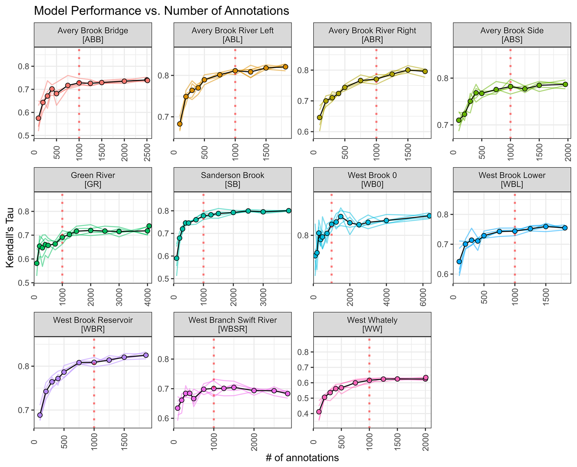
Figure 8 Model performance as a function of the number of annotations used to train the model. Colored lines indicate individual scaling experiments (n = 5); the black line and points indicate mean performance. The dotted vertical line shows 1000 annotations. Axis limits vary among panels. Performance computed on daytime (07:00–19:00 local time) photos only. Subplots labeled with site name and number described in Table 1.

4 Discussion

We find that a low-cost methodology for monitoring relative streamflow dynamics in headwater streams is effective at characterizing interannual hydrologic events and short-term storm responses at the stream sites within our study. Based on our encouraging results, we anticipate that the approach will provide a valuable alternative to traditional stream gaging methods when relative streamflow dynamics information is needed, but the streamflow discharge is not required. The person-generated annotation, model performance patterns, and sensitivity analysis performed in this study have implications for how we refine the modeling approach and provide guidance to users as this platform evolves.

This study was our first insight into annotator accuracy. In a previous study outlining the SRE method (Gupta et al., 2022), the ability to correctly rank the image pair was varied systematically using simulations. In that study, in addition to a perfect annotator that always ranked the image pair correctly, the authors simulated annotations with varying ability to discern between streamflow differences in the photo pair. The thresholds they tested included 10 %, 20 %, and 50 % of the lesser discharge. The authors found that a less discerning annotator had to perform more annotations to train a model that reached similar performance to one trained on annotations from a more discerning annotator. However, these annotators could not make mistakes; incorrect labels were not introduced. Conversely, in this study, people performed annotations. While the overall accuracy of the annotators at individual sites ranges from 84 %–96 %, these accuracy statistics obscure another feature of annotation; annotators are near perfect at distinguishing large differences in flow and less accurate at distinguishing small differences in flow. Even when provided with a “same” button and a “don't know” button, annotators make mistakes at small differences in flow. This is likely due to the difficulty of the task in the presence of camera angle shifts, obscuring vegetation, changes in channel morphology, and the fact that it is simply difficult to discern small differences in streamflow visually. Annotation performance in our dataset followed similar patterns for 2 annotators and across 11 camera sites, such that all data could be reasonably fit with a single mathematical function (see Fig. 4). Future studies could use this function to simulate annotator performance more accurately than previous threshold-based simulations. This study primarily relied on annotations from two individuals with similar backgrounds, and a single annotator worked on each site, resulting in a potential conflation of annotator and site variability. Future work using larger annotation datasets or designed common annotation sets could better assess the range of skill across individuals and backgrounds. In this study we used streamflow gage observations to quantify annotator and model performance. Where observations are not available, annotator performance could be assessed using multiple annotators assessing the same image pairs. Model performance could be evaluated using post hoc human review using a similar approach to annotation.

This study's models, trained with person-generated annotations, produced a time series of streamflow percentile estimates analogous to a relative hydrograph that can be used to monitor the timing, duration, and relative magnitude of hydrologic events (Fig. 6; the Supplement). All performance metrics in this paper are provided for the original approximately 15 min interval frequency of the imagery and streamflow data, though the time series plots of model predictions do show substantial sub-daily variability in streamflow percentiles. For example, at times in late 2023, daily percentiles at the Avery Brook Bridge site consistently range from nearly 25 % to 90 % (Fig. 6). A review of individual images during times of high sub-daily percentile variability shows that outliers in model prediction can be introduced by the presence of sun glare on the camera, vegetation blocking the camera view, twilight conditions, fog/haze, and other factors that present the model with unfamiliar views (Sect. S3 in the Supplement). Since we allow annotators to exclude photos that are obscured, the model is not trained on these images, which leads to poorer performance. A focus of future work on identifying and excluding these images will likely reduce the variability at a sub-daily scale resulting from poor images. Even in the presence of these features, the daily mean values plotted correspond well with major hydrologic events, such as a drought in the summer of 2022 that affected the region, and individual storm events. Users of these modeled relative streamflow data could create daily mean values if they were interested in results at this scale. However, we report sub-daily model performance because the headwater streams that are a focus of this work are highly responsive to storm events, and it is also important to capture these events to understand and characterize streamflow dynamics.

Where available, this study found lower model performance for the “test-out” period than the `test-in` period, though the degree of performance decrease varied among sites. Even for the four co-located sites on Avery Brook the decrease in model performance from “test-in” to “test-out” varied substantially (Fig. 5). We believe this may be due to a combination of new camera views not seen in training and the fact that the “test-out” period often included winter, which can be a period of lower performance due to snow obscuring the stream. The general approach we took may be limited in its ability to describe the magnitude of out-of-distribution streamflow in the “test-out” period, but due to the limited availability of sites with “test-out” periods, we are unable to draw conclusions that might hold true for other sites. Creating models from longer paired imagery and streamflow records with more extensive “test-out” periods will support future efforts to minimize performance loss for the “test-out” period, likely through improvements in the image augmentation steps of the modeling procedure.

Model performance among sites seems to be driven by the variability in the streamflow during the monitoring period. We find that annotator and model performance at sites that have very steady flow is low relative to sites experiencing wide variation in observed streamflow. To some extent this is a consequence of Kendall's Tau as a performance metric, where a small range in the overall data causes small fluctuations in stream discharge to manifest as large fluctuations in rank percentile. However, physical characteristics matter; for this method to perform well the stream needs to have visible changes in streamflow during the training period. The site in this study with the lowest streamflow coefficient of variation, West Whately, also had a very low stream depth such that the water surface was difficult to see within a meandering channel and in the presence of leaves. Future work with more sites will be better positioned to evaluate how camera stability, flow variability, and other factors affect annotation and model performance. This study refines user guidance in two important ways. First, our results suggest that sites that experience a wide range of flows (or for enough time that a wide range of flows are experienced) will have higher model performance. Second, since our simple camera stability classification has a weak association with annotator accuracy and no significant relationship with model performance, the method is robust to slight changes in camera angle and can still be used if these shifts are present. However, the limited three-category approach in this study may limit the findings. More complex frame-tracking algorithms to quantify camera stability (e.g., Ljubičić et al., 2021) could further improve insights into the robustness of the method to camera shifts.

A key requirement of this methodology is the need for a person to perform annotations on the imagery datasets. Anecdotally, users typically annotate at an average pace of 1000 image pairs per hour using the interface. However, in practice, annotations are typically performed in smaller batches (100–200 images per batch) with breaks in between, resulting in a slower effective pace. The sensitivity analysis performed in this study helps evaluate the number of annotations to reach near-optimal model performance while not wasting annotator effort. For our available sites and annotation datasets we approximate 1000 annotations as a reasonable guideline when creating a new model. While there is slight variability among the sites, the consistency of the shape of the curves shown in Fig. 8 suggests that a single guideline is reasonable. The number of annotations may also be controlled by factors not included in the sensitivity analysis, such as the record length and annotator accuracy. Additional sensitivity analyses, likely using synthetic annotation datasets, could further refine the guideline for how many annotations to perform when developing ranking models at new sites.

The output of the deep learning model is a relative flow percentile estimate. Although streamflow discharge (i.e., a flow rate with units of volume per time) is a more familiar metric, relative flow has value for several applications. With relative flow estimates we can (1) evaluate the duration and timing of disturbances such as drought and flood events, (2) provide inputs to statistical models such as ecological population models that may not require absolute streamflow accuracy, (3) establish or confirm relationships between streamflow at a study reach and at other nearby locations, (4) evaluate the ability of hydrologic models to simulate streamflow dynamics at a study reach, and (5) provide the basis for counting the exceedance of site-relevant thresholds (for example, the number of times a roadway is inundated or the number of times an intermittent stream is active). These outputs are aligned with the work of other authors to use semiquantitative observations to study headwater streams, for example stream connectivity (Bellucci et al., 2020; Kaplan et al., 2019). Nevertheless, some applications require absolute flow, and in future work we intend to explore approaches to transform relative flow estimates produced by the SRE model into absolute streamflow discharge estimates, either by periodically measuring discharge at the site or by using discharge data from nearby locations (if available). For now, we intend to communicate the appropriate use of these relative percentile estimates and avoid implying that streamflow discharge is produced by this work.

Because our study reports relative rather than absolute streamflow, it is difficult to directly compare our model performance against other similar work. We report our performance with the rank-based Kendall Tau value, which is analogous to a nonparametric R² value appropriate for our model outputs. Similar studies using time lapse camera imagery to monitor rivers focus on reproducing point-in-time stage observations, often using in-channel calibration targets such as staff gages (Chapman et al., 2022; Eltner et al., 2018; Gilmore et al., 2013; Kim et al., 2011; Lin et al., 2018; Nguyen et al., 2009). These studies vary in approach, though typical steps include identifying the target and water surface, performing an orthorectification of the image into real-world space, and conducting a measurement of a visual target. Typically, authors report sub-centimeter-level accuracy. For example, a field study of uncertainty in one system reported ±5 mm accuracy at the 90 % confidence interval in a tidal marsh environment with tranquil waters, though the authors noted this system was unsuited to fast-moving turbulent water such as the mountainous headwater streams in our dataset (Birgand et al., 2022). A deep-learning water-segmentation-based approach reported Spearman correlations between independent stage measurements ranging from 0.57 to 0.94 at a single well-characterized gage site in eastern Germany (Eltner et al., 2021). We note these performance metrics reported by other similar studies, though due to differences in the model outputs our performance metrics are not directly comparable. Where evaluated in the field, most similar studies report results for single sites and/or for durations of less than 1 year (Birgand et al., 2022; Eltner et al., 2021; Leduc et al., 2018; Liu and Huang, 2024; Schoener, 2018), making this study's multi-year monitoring of 11 camera sites a comparatively robust representation of model performance.

This work, while promising, is limited in a few important ways. Primarily, this system is not (and is not intended to be) a replacement for high-accuracy stream stage or discharge measurements that are required for many applications such as computing streamflow trend, calculating nutrient loads, or supporting water management decision making. Users of this system must understand the relative nature of the results and determine if relative streamflow hydrographs are suitable for their application; we envision suitable applications to include habitat characterization, aquatic species population dynamics modeling, refining process understanding in small catchment studies, intermittent stream monitoring, and characterizing event (i.e., flood or drought) timing. In this study, model training and prediction is limited to daytime imagery, which we defined simply as between 07:00 and 19:00 local time. While these cameras also have infrared flash that illuminates the channel, the degree to which the scene is visible at night varies significantly between sites. The imagery at night becomes grayscale, and we expect that different portions of the imagery become important for a model. It is unclear if nighttime imagery is best modeled with both day- and nighttime imagery or if a night-only model should be trained, and future work may investigate this. We also noticed that lens fog, camera glare, vegetation blockages, and other visual impediments had a negative impact on model performance. When present, these image issues typically resulted in abrupt high or low outliers in model score. For this analysis we retained these predictions as part of the overall evaluation. We expect computer vision algorithms to detect and remove these images, which would further improve model performance. Data collection on the Flow Photo Explorer platform enables users to flag “bad” images during data annotation, which will enable us to develop outlier detection algorithms for this purpose.

5 Conclusions

The camera-based methodology discussed here offers a novel approach to estimating relative streamflow. Its low cost and effort requirements should make it feasible to create dense observation networks to fill gaps in existing streamflow monitoring observations and thereby improve understanding of relative streamflow dynamics in headwater streams. While currently limited to estimates of relative streamflow trained as single-site models, we expect continued improvements that will expand the applicability and improve the ease of training models for new locations. The purpose of this paper was to answer questions based on an initial set of monitoring stations. These findings will guide further development of the Flow Photo Explorer integrated web platform that allows users to upload, annotate, model, and interpret headwater stream imagery. To summarize, this study answers the following questions:

• 1.

  How accurate are people at ranking images by streamflow? Overall annotation accuracy of image pair ranking ranged from 84 % to 96 % (average of 92.2 %) among the 11 camera sites. While limited to primarily two individuals, we see that our annotators are nearly 100 % accurate at ranking stream image pairs when there are large differences in observed streamflow. Small differences in streamflow between image pairs were more difficult for the annotators to identify. Due to consistency among sites, the accuracy of person-generated streamflow annotations used in this study can be reasonably simulated with a single globally fit equation.

• 2.

  How accurate are image-derived relative hydrographs developed using person-generated annotations? Kendall's Tau values for streamflow percentile predictions ranged from 0.6 to 0.83 for unannotated days within the training period. These represent the retrospective model performance. Lower performance was observed for predictions on data collected after the training period, which may have a different distribution of streamflow or changes to the image scene. Where available, Kendall's Tau values for the post-training period range from 0.34 to 0.74.

• 3.

  Which factors influence ranking model accuracy and indicate which unmonitored catchments would be suitable for low-cost camera monitoring? The primary factor describing among-site differences in performance was streamflow variability. Describing relative streamflow changes in streams with steady flow was challenging, in part due to our relative (percentile-based) metrics of performance. We expect better performance for streams that exhibit large stage variations, are seasonally dry, or have large seasonal variations in flow.

• 4.

  How many person-generated annotations are required to achieve stable ranking model performance? An experiment indicated that for most sites there were diminishing improvements in performance after about 1000 pairwise annotations. We therefore conclude this is a reasonable minimum number of annotations to develop a ranking model.