Improving model calibrations in a changing world: controlling for nonstationarity after mega disturbance reduces hydrological uncertainty

Model simulations are widely used to understand, predict, and respond to environmental changes, but uncertainty in these models can hinder decision-making. The simulation of hydrological changes after a forest fire is a typical example where process-based models with uncertain parameters may inform consequential predictions of water availability. Different parameter sets and meteorological forcing assumptions can yield similarly realistic simulations during model calibration but generate divergent predictions of change, a problem known as “equifinality.” Despite longstanding recognition of the problems posed by equifinality, the implications for environmental disturbance simulations remain largely unconstrained. Here, we demonstrate how equifinality in water balance partitioning causes compounding uncertainty in hydrological changes attributable to a recent 1540 km² megafire in the Sierra Nevada mountains (California, USA). Different model calibrations generate uncertain predictions of the 4 year post-fire streamflow change that vary up to six-fold. However, controlling for nonstationary model error (e.g., a shift in the model bias after disturbance) can significantly (p < 0.01) reduce both equifinality and predictive uncertainty. Using a statistical metamodel to correct for bias shift after disturbance, we estimate a streamflow increase of 11 % ± 1 % in the first four years after the fire, with an 18 % ± 4 % increase during drought. Our metamodel framework for correcting nonstationarity reduces uncertainty in the post-fire streamflow change by 80 % or 82 % compared to the uncertainty of pure statistical or pure process-based model ensembles, respectively. As environmental disturbances continue to transform global landscapes, controlling for nonstationary biases can improve process-based models that are used to predict and respond to unprecedented hydrological changes.

1 Introduction

Calibration – systematic adjustment of model parameters to improve simulation accuracy.

Disturbance – an event that changes an environmental system from one state to another.

Equifinality – the production of similar results for different reasons.

Stationarity – the invariance of a statistical property across different time periods.

Environmental disturbances (e.g., forest fires, other vegetation mortality events, floods, anthropogenic land cover conversion, etc.) can alter the structure and function of ecohydrological systems (Zehe and Sivapalan, 2009; Ebel and Mirus, 2014; Buma, 2015; Johnstone et al., 2016). Climate change and environmental disturbances introduce nonstationarity into the hydrological cycle, which is disrupting longstanding statistical approaches to water resource and risk management (Milly et al., 2008, 2015; Hirsch, 2011; Salas et al., 2012; Yang et al., 2021).

Pure statistical methods (e.g., regression models lacking an explicit physical foundation) can sometimes detect streamflow changes attributable to environmental disturbance by comparing measurements to a stationary model, which represents a no-disturbance counterfactual. In this context, a “counterfactual” refers to a hypothetical scenario in which a particular disturbance did not happen, so comparing the actual post-disturbance behavior to the modeled counterfactual enables attribution of disturbance effects. Statistical change attribution is generally applied across many years and numerous sites (e.g., Goeking and Tarboton, 2022a; Hampton and Basu, 2022; Williams et al., 2022) or in careful paired watershed studies to overcome climate/weather variability (e.g., Bart, 2016; Manning et al., 2022; Johnson and Alila, 2023; Kang and Sharma, 2024). However, in a single watershed with a short post-disturbance record, pure data-driven statistical approaches are inherently limited. Crucially, many water management decisions (e.g., reservoir release schedules) are made on a per-watershed and per-year basis, so large-scale retrospective statistical assessments of disturbance effects may not provide actionable insights in any particular watershed.

Spatially distributed process-based hydrological models, and related land surface or Earth system models, are a widely accepted tool that can overcome some limitations of statistical disturbance attribution (Fatichi et al., 2016; Pongratz et al., 2018; Fisher and Koven, 2020). Because interannual climate variability often obscures hydrological changes caused by disturbance, counterfactual model experiments using an undisturbed control are a cornerstone of ecohydrological disturbance attribution studies (e.g., Moreno et al., 2016; Saksa et al., 2017; Boisramé et al., 2019; Meili et al., 2024). Moreover, key process representations (e.g., flow routing and the snowpack energy balance) are expected to generalize beyond observed conditions, providing a basis for the prediction of hydrological responses to out-of-sample events including extreme storms (e.g., Huang and Swain, 2022), decadal-scale climate change (e.g., Tague et al., 2009), and unprecedented “megafires” (e.g., Abolafia-Rosenzweig et al., 2024). In this context, a megafire is any wildfire in excess of 400 km² (Ayars et al., 2023).

We lack landscape-scale observations of meteorology and many other important environmental properties, so it is typically challenging or impossible to setup a single “best” model without a degree of trial-and-error. Therefore, model parameters are often estimated through calibration. Equifinality arises during calibration when different parameter sets yield similar realizations of observable phenomena (Beven, 1993, 2006; Ebel and Loague, 2006). Recognizing that equifinality may preclude the possibility of picking a single “best” parameter set, some modelers advocate for using a “behavioral” ensemble based on subjective goodness-of-fit criteria in a generalized likelihood uncertainty estimation (GLUE) framework (Spear and Hornberger, 1980; Beven and Binley, 1992; Her and Chaubey, 2015; Vrugt and Beven, 2018).

Equifinality implies process uncertainty (Grayson et al., 1992; Khatami et al., 2019). For example, total evapotranspiration (ET) is the sum of overstory and understory transpiration, interception loss, soil evaporation, snow sublimation, and other vapor fluxes; equifinal parameter sets may produce the same total ET with different partitioning between constituent fluxes (Franks et al., 1997; Birkel et al., 2024). Because each vapor flux component can respond differently to disturbance (Goeking and Tarboton, 2020), equifinal parameter sets may produce divergent predictions when the model is perturbed beyond the calibration space (Seibert and McDonnell, 2010; Melsen et al., 2018).

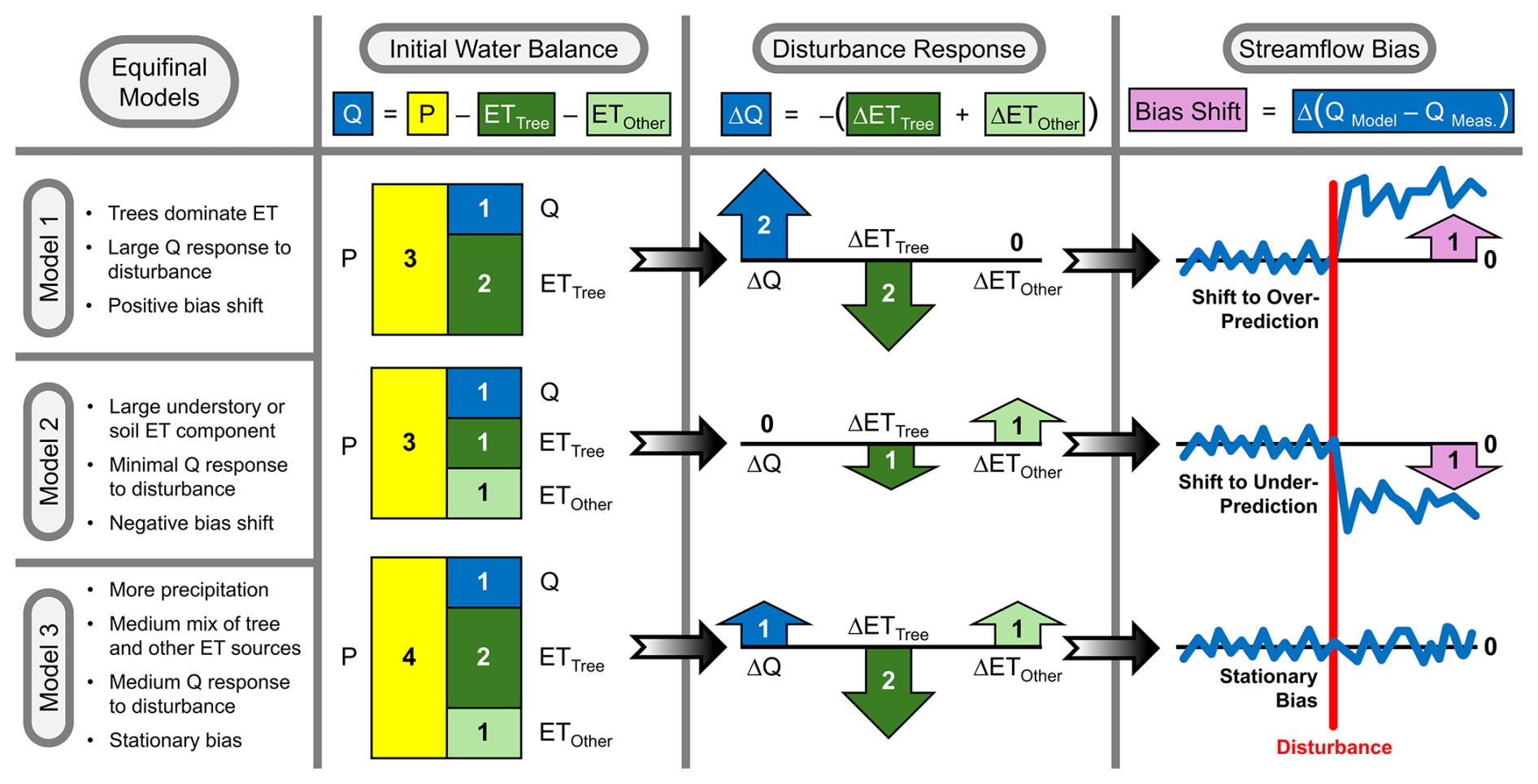
Figure 1 Conceptual model illustrating how equifinality in the modeled water balance may lead to uncertainty in the streamflow response to disturbance, and how we expect this to manifest in a measurable “bias shift” after a discrete disturbance. Numbers are indicative and not intended to represent actual disturbance magnitudes. In the “initial water balance” panel, we assume that all three models closely match pre-disturbance streamflow, with uncertain precipitation and evapotranspiration (ET) components counterbalanced to produce $Q_{\text{Observed}}=Q_{\text{Modeled}}=\mathrm{1}$ (normalized annual units). After a disturbance (e.g., a wildfire) reduces ET_Tree, the different models predict various degrees of streamflow change, which is mediated by the potential for compensating increases in ET_Other (e.g., soil evaporation and understory ET). In the “disturbance response” panel, the arrows illustrate the direction and magnitude of the water balance changes predicted by each model. In the “streamflow bias” panel, the resulting model predictions are compared to measured streamflow, showing how some models could exhibit a bias after disturbance due to uncertain estimation of water balance changes. In this hypothetical example, we assume that Q_Observed increases by 1 unit after disturbance, matching the prediction of Model 3.

We illustrate the hypothesized interaction of equifinality, disturbance, and bias (non)stationarity using a conceptual water balance model (Fig. 1). Example models of the pre-disturbance water balance each achieve the same mean pre-disturbance streamflow (Q), which is forced to approximately match Q observations through model calibration. Due to equifinality, there is residual uncertainty in the bias-corrected total precipitation (P) and the partitioning of ET between transpiration and interception from tree canopies (ET_Tree) and other vapor fluxes (ET_Other, e.g., understory ET and soil evaporation). When a disturbance such as a fire reduces ET_Tree, the streamflow response is sensitive to the initial ET_Tree magnitude (and hence the potential ET reduction) as well as the degree to which ET_Other responds to increased soil water availability. The three examples show cases where ET_Other does not respond to the disturbance (Model 1), increased ET_Other fully compensates for reduced ET_Tree (Model 2), or increased ET_Other only partly compensates for reduced ET_Tree (Model 3). Intuitively, these hypothetical model responses are connected to the pre-disturbance balance of ET_Tree and ET_Other, which primes some models to predict a larger or smaller compensation effect. Over- or under-estimation of the resultant streamflow change (ΔQ) manifests as a positive or negative “bias shift” after disturbance. The bias shift metric, as defined here, is a special discrete case of the more general concept of nonstationarity. In a system with changes that occur over longer time periods (in contrast to the discrete disturbance shown in Fig. 1), a different stationarity metric would be necessary to account for incremental changes. In the present study, zero bias shift after disturbance implies stationary error overall.

We build on this conceptual example of the interaction between equifinality, disturbance, and nonstationarity (Fig. 1) to consider how the bias shift metric can help select parameter sets with enhanced physical fidelity and greater predictive confidence. The initial water balance of Model 1 is dominated by ET_Tree, leading to a large streamflow gain and a positive bias shift (tendency toward over-prediction of post-disturbance streamflow). Conversely, Model 2 has a large ET_Other component, which compensates for the comparatively small reduction in ET_Tree, leading to a negligible streamflow gain and a negative bias shift (tendency toward under-prediction of post-disturbance streamflow). Finally, Model 3 has more precipitation than the other models and a more balanced combination of ET_Tree and ET_Other, leading to a medium streamflow gain and stationary bias. In this case, Model 3 should be preferred due to its negligible bias shift, which would help achieve a better prediction of ΔET and ΔQ and also help constrain uncertainty in the underlying parameterization.

As illustrated in Fig. 1, meteorological uncertainty (e.g., a precipitation bias) can interact with uncertain model parameterizations, contributing to uncertainty in the streamflow response to disturbance (Elsner et al., 2014). Basin-scale meteorology data are highly uncertain in mountain regions (e.g., Lundquist et al., 2015; Henn et al., 2018; Schreiner-McGraw and Ajami, 2022), and whatever assumptions are made about the meteorology can cause compensating inaccuracies with other calibrated parameters (Elsner et al., 2014). For example, overestimating basin-scale precipitation may cause the model to simulate a larger ET_Tree component and a corresponding large change in post-fire water balance partitioning (Model 3 in Fig. 1), whereas underestimating basin-scale precipitation could limit the predicted post-fire streamflow change since the pre-fire P − Q residual is smaller (Models 1–2 in Fig. 1). From a Bayesian perspective, we can view the data and model as a combined inferential system, which enables us to constrain uncertainty in the interactions between uncertain meteorology and uncertain hydrology by generating suitable ensemble samples (Kavetski et al., 2003). Thus, uncertainty in the meteorological forcing data will contribute to uncertainty in our estimate of post-fire streamflow changes.

Equifinality has been neglected in many process-based simulations of environmental disturbance. In contemporary studies, single parameter sets are sometimes used with or without site-specific calibration (e.g., Furniss et al., 2023; Abolafia-Rosenzweig et al., 2024). When parameter ensembles are used, uncertainty propagation is commonly limited to subsurface parameters and meteorological biases (e.g., Shields and Tague, 2012; Saksa et al., 2017; Boisramé et al., 2019). We expect that latent uncertainty in vegetation parameters may contribute an unconstrained source of uncertainty in studies of ecohydrological disturbance that do not account for vegetation parameter equifinality. Conversely, model equifinality can be reduced by leveraging additional types of information beyond traditional streamflow calibration metrics (Kelleher et al., 2017). One unexplored approach to equifinality reduction is evaluating the stationarity of model biases after environmental disturbance (e.g., bias shift in Fig. 1), which we consider here.

In this study, we leverage a large wildfire as a “natural experiment” to test the hypothesis that quantifying stationarity across pre- and post-disturbance periods can reduce equifinality and improve the predictive confidence of a process-based hydrological model. Specifically, we apply the Distributed Hydrology Soil Vegetation Model (DHSVM, Wigmosta et al., 1994) to simulate streamflow changes attributable to the Creek Fire in the Sierra Nevada mountains (California, USA), which burned 56 % of the forested area in our 4244 km² study watershed (Stephens et al., 2022; Ayars et al., 2023). We expect that this drastic landscape-scale environmental disturbance should have a clear impact on regional-scale water fluxes, providing a natural experiment to test whether ecohydrological model process representations are robust to environmental disturbance. We leverage a multi-objective calibration of vegetation, snow, subsurface, and meteorological bias-correction parameters to address two research questions:

1. How does calibration equifinality impact process-based simulations of the hydrological response to a megafire?

2. Can we reduce equifinality and uncertainty by testing the model's representation of hydrological change?

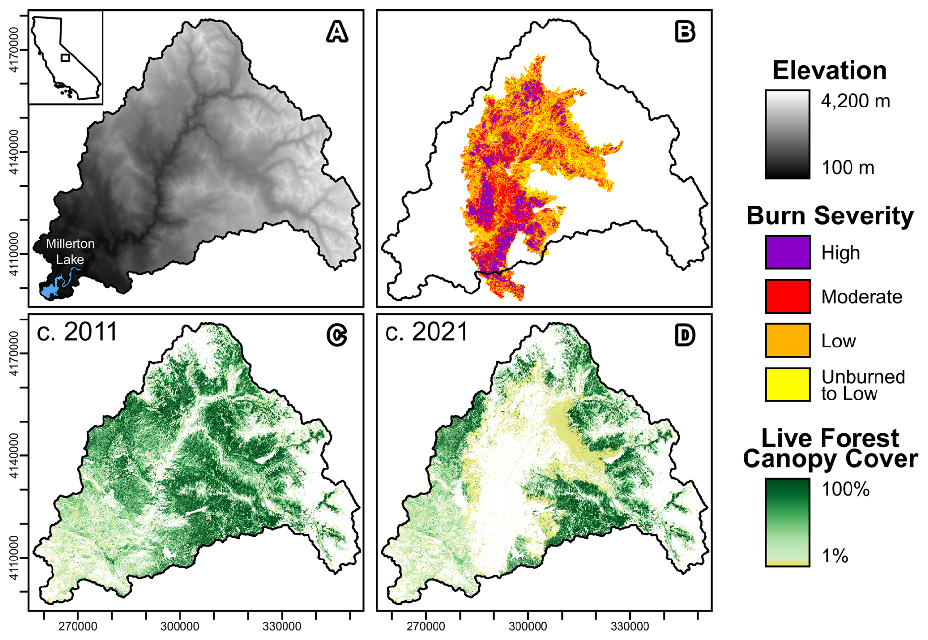
Figure 2 Maps of the study watershed: (A) elevation and watershed location in the US State of California, (B) 2020 Creek Fire burn severity, (C) pre-fire and (D) post-fire forest canopy cover. Tick marks indicate 10 km intervals.

2 Methods

2.1 Study Area and Data

Our study watershed encompasses the Upper San Joaquin River Basin above the outlet of Millerton Lake, a total of 4244 km² with an elevation range of 100 to 4200 m (Fig. 2A). The 2020 Creek Fire burnt 1540 km² of mixed conifer and scrub forest, including 1481 km² within the study watershed (56 % of the forested watershed area). Landsat-based data from Monitoring Trends in Burn Severity (MTBS, Fig. 2B) indicate that 16 % of the Creek Fire exhibited high burn severity and 30 % exhibited moderate severity (Eidenshink et al., 2007; MTBS Project, 2022). However, using a longer time period for pre- and post-fire imagery, Stephens et al. (2022) estimate 41 % high severity and 35 % moderate severity, illustrating the proliferation of uncertainty in disturbance assessments.

We represent fire disturbance in DHSVM by adjusting maps of vegetation properties. Canopy cover maps are projected to our selected DHSVM resolution of 90 m using nearest-neighbor resampling to preserve the categorical attribute of tree presence/absence. The Landsat-based RCMAP data provide yearly fractional cover estimates for trees and shrub/herbaceous vegetation at 30 m resolution (Rigge et al., 2021a, b). We use the 2011-era RCMAP data as a pre-fire baseline and the 2021-era RCMAP data to capture the effects of the 2020 Creek Fire (Fig. 2C and D). We also update the vegetation maps in 2013, 2014, and 2018 to reflect smaller fires in those years. The DHSVM vegetation maps are updated on 1 October in the year of a fire, i.e., about one month after the September 2020 Creek Fire ignition. The 1 October date is used for annual model updates because this date represents the start of a new water year, and Sierra Nevada watersheds are typically near their driest condition around this time of year, which limits the impact of model changes on simulated hydrological fluxes. Additionally, fires typically burn in the late summer in the Sierra Nevada, so the 1 October date is close to the typical end of the fire season. However, studies focused on short-term post-fire effects may need to update vegetation maps on the dates immediately after each fire, or even multiple times as a fire progresses (e.g., the Creek Fire burned for several months). Vegetation is classified based on the species (when available) or functional type (e.g., mixed conifer forest) using Landfire data (2022), and abiotic land surface classes are derived from NLCD (Dewitz and U.S. Geological Survey, 2019). Landfire and RCMAP provide tree and shrub height data, respectively. Tree leaf area index (LAI) is estimated empirically from fractional cover following Pomeroy et al. (2002), which is reproduced as Eq. (1) of Goeking and Tarboton (2022b). Satellite-based optical LAI estimates are highly uncertain in mountain environments due to saturation at the high LAI values often present in mature conifer forests and the inability to resolve 3-dimensional canopy structure that controls LAI (Zolkos et al., 2013; Winsemius et al., 2024). Thus, we use the fractional cover relationship to constrain the spatial patterning of LAI, but the uncertain LAI magnitude is estimated heuristically through calibration. Vegetation transpiration is calculated by DHSVM based on the vegetation type and local weather, soil moisture, and light in each grid cell (Wigmosta et al., 1994). Baseline values of minimum stomatal resistance are estimated from species-level field studies as detailed in the Supporting Information of Boardman et al. (2025) and refined by calibration relative to baseline (Sect. 2.2).

Spatial maps and parameter values for DHSVM are collated from a wide range of literature and field studies, as detailed in Boardman et al. (2025). We briefly summarize key setup procedures here. Subsurface properties are estimated by disaggregating regional soil survey databases (Gupta et al., 2022; Soil Survey Staff, 2022) using Random Forest models trained on topographic metrics (Breiman et al., 2002). In the updated version of DHSVM used here, streamflow in channels is bidirectionally coupled to the groundwater level in each grid cell, and the maximum network extent is derived from the National Hydrography Dataset (U.S. Geological Survey, 2019) with channel geometry from regional regressions (Bieger et al., 2015). Meteorological data from gridMET (Abatzoglou, 2013) are disaggregated to a 3 h timestep using MetSim (Bennett et al., 2020). Modeled snowfall is distributed in proportion to the pixel-wise maximum observed snow water equivalent (SWE) pattern derived from Airborne Snow Observatory (ASO) data in the study watershed (Painter et al., 2016), which implicitly accounts for snow transport (Vögeli et al., 2016). Regional snow/rain partitioning parameters are adopted from Sun et al. (2019).

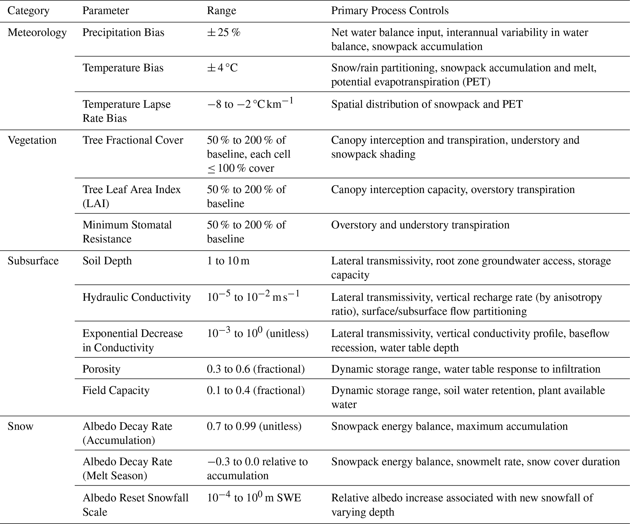
Table 1 Prior ranges and process controls of DHSVM parameters calibrated in this study. All vegetation and subsurface parameters listed here are defined by spatially variable maps, and calibration ranges determine the area-average value around which the pattern is rescaled.

2.2 Model Calibration

We calibrate 14 sensitive and uncertain parameters in DHSVM that control aspects of the meteorology, vegetation, subsurface, and snowpack dynamics (Table 1, Fig. S4 in the Supplement). While most of these parameters are widely recognized as suitable for calibration (Cuo et al., 2011; Du et al., 2014), precipitation and temperature biases are less frequently included in the calibration of distributed process-based models despite considerable uncertainty in gridded meteorological data. Among gridded meteorological datasets, there is a mean relative difference of 21 % for annual precipitation in our study watershed (Henn et al., 2018), and misestimation of large storms can lead to yearly biases of about 20 % across the Sierra Nevada (Lundquist et al., 2015). Similarly, gridded meteorological datasets have mean air temperature differences as large as ± 8 °C in the Sierra Nevada, and basin-average uncertainty is lower but still on the order of several °C (Schreiner-McGraw and Ajami, 2022). Compensation between unknown errors in the meteorological data, model structure, and parameter calibration can potentially contribute to spurious goodness-of-fit metrics with hidden physical deficiencies. This is especially the case in environmental disturbance studies, as we expect that interactions between meteorological uncertainty and parameter equifinality may contribute to the overall uncertainty of disturbance simulations (Fig. 1). Critically, this uncertainty would remain hidden if meteorological biases were assumed to be negligible. Because perfectly resolving the weather data with infinite precision is not feasible across a large, rugged mountain region, the robust approach is to propagate meteorological uncertainty into our final results (the post-fire hydrological change in this case), so that our conclusions include the quantified uncertainty caused by the model–data–calibration interaction. We view the combined meteorological data and hydrological model as a single inferential system, thereby acknowledging that the meteorological data themselves are based on various uncertain observations and empirical model assumptions (Abatzoglou, 2013). In a Bayesian context, the goal of our calibration can be understood as sampling the probability of the calibration data (streamflow and snowpack observations) given a particular combination of model parameters and meteorological assumptions: $P(\text{streamflow}+\text{snowpack\hspace{0.17em}\hspace{0.17em}observations}\mathrm{|}\text{model}+\text{meteorology})$. Because we lack a closed-form likelihood function for spatially distributed hydrological models like DHSVM, we estimate the unknown parameters of this whole weather-model system using an informal approximation based on traditional hydrological model calibration objective functions (Beven and Binley, 1992).

Multiple parameters combine to control simulated processes. For example, area-average LAI (related to total interception loss) is the product of tree-scale LAI with grid-scale fractional cover. Tree transpiration is determined by fractional cover, LAI, stomatal resistance, available soil water (related to subsurface parameters), and other factors. Lateral transmissivity in the saturated subsurface is controlled by three parameters: soil depth, surface hydraulic conductivity, and the exponential decrease in conductivity with depth. Cross-compensation among interrelated parameters thus contributes to equifinality. Within our 14-dimensional calibration space, 23 parameter pairs have correlations that are significant at p < 0.05 (Fig. S1 in the Supplement). Furthermore, perturbing one aspect of the model can lead to cascading effects due to the coupling of ecohydrological processes and spatial water connectivity in the model. For example, lateral hydraulic conductivity is coupled to vertical conductivity by anisotropy ratios dependent on the soil textural classification (Fan and Miguez-Macho, 2011), so calibrating lateral conductivity also influences groundwater recharge rates from losing stream reaches, which in turn can affect soil evaporation and transpiration from riparian trees. Spatial heterogeneity in modeled soil and vegetation properties (Sect. 2.1) further complicates all of these interactions, e.g., different parts of the landscape are relatively more sensitive to calibration of different parameters depending on the baseline map patterns.

Table 2 Calibration objective functions used in this study with descriptions of the primary hydrological signatures constrained by each objective. The best (worst) value given here is the lowest (highest) error achieved by any of the Pareto-efficient parameter sets in our calibrated 30-member behavioral ensemble. NSE = Nash–Sutcliffe Efficiency, RMSE = root mean square error, MAPE = mean absolute percent error.

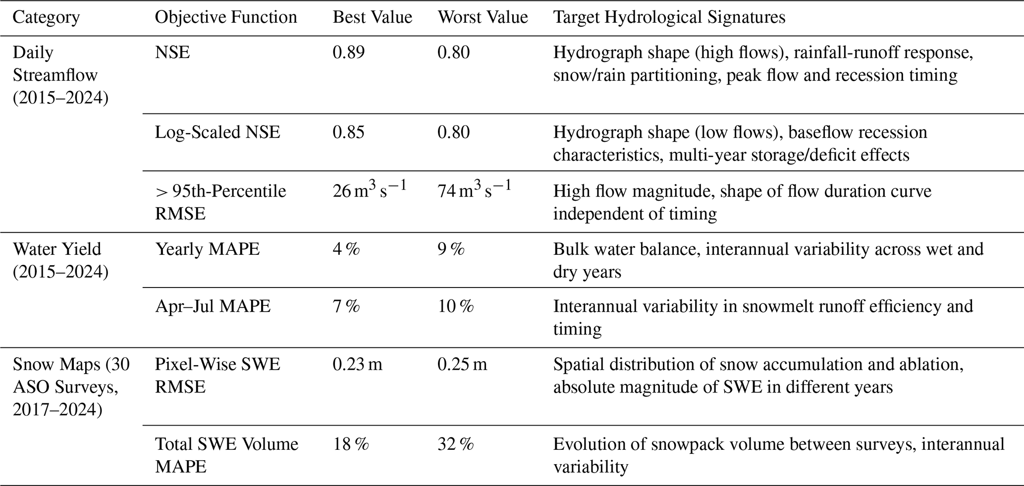
Given the complexity of expected interactions, we define seven objective functions to constrain parameters based on different hydrological signatures (Table 2). Streamflow is estimated at the outlet of Millerton Lake (Fig. 2) by reconstructing observations to remove the effects of artificial flow regulation (California DWR, 2024). Millerton Lake unimpaired outflows are estimated assuming sub-daily surface routing times by summing the daily change in storage, canal and dam releases, surface evaporation, and storage changes at eight smaller upstream reservoirs (Huang and Kadir, 2016). Note that the reconstructed streamflow timeseries used in this study (called “full natural flow” by the California Data Exchange Center) is based on an explicit mass balance equation applied directly to the respective storage and flow measurements, not model output, unlike various other meanings of “natural flow” that are sometimes applied to California water datasets (Huang and Kadir, 2016). The reconstructed streamflow timeseries (hereafter “observed streamflow”) represents the actual effects of the Creek Fire (and other disturbances) because the reconstruction procedure is directly based on measurements at specific diversion, storage, and outflow points, which are directly responsive to the basin hydrological conditions. Three objective functions are based on a cleaned version of this daily streamflow timeseries (spurious negative values during low-flow periods and other missing values are imputed). Two objective functions similarly target annual percent error in the annual water yield and the April–July water yield, which is a well-established benchmark for snowmelt runoff modeling in the Sierra Nevada (Pagano et al., 2004). Two objective functions are based on the 8 year (2017–2024), 30-survey database of ASO SWE maps in the study area, targeting both the spatial distribution at the 90 m grid scale and the percent error in total volume across surveys. Hydrograph and water yield objectives are calculated for water years 2015–2024, which includes 6 years before and 4 years after the Creek Fire. By calibrating across this disturbance (vegetation maps updated during calibration), we automatically reject parameter sets that fail to provide reasonably accurate estimates of both pre- and post-fire streamflow.

To efficiently sample behavioral parameter sets from the 14-dimensonal space of potential interactions, we apply a multi-objective Bayesian optimization scheme (Jones et al., 1998). After an initial Latin hypercube sample of 320 parameter sets (Dupuy et al., 2015), we perform parallel particle swarm optimization (Kennedy and Eberhart, 1995; Zambrano-Bigiarini et al., 2013) using the expected hypervolume indicator (Emmerich et al., 2011; Binois and Picheny, 2019) to sample promising parameter sets based on Gaussian Process surrogate models of the objective function response surfaces (Roustant et al., 2012). After six optimization generations, we have tested a total of 600 parameter sets (n.b. this requires ∼ 950 d of CPU time on 2.5 GHz servers, but the elapsed wall-clock time is several weeks because multiple parameter sets are tested in parallel). While this number of tested parameter sets may seem small by conventional standards considering the 14-dimensional search space, we note that each new parameter sample is selected after an independent optimization procedure using 100 to 1000 particle swarm samples from the objective function surrogate models. Thus, our overall calibration explores the objective function tradeoffs across more than 160 000 parameter sets, but only 600 of these are actually tested in DHSVM. Because testing hundreds of thousands of parameter sets directly in DHSVM would require prohibitive amounts of computational expense, this Bayesian surrogate optimization procedure is essential for efficiently selecting parameter sets that have the best likelihood of substantially improving the Pareto frontier.

As expected for any high-dimensional multi-objective optimization problem, there is no single “best” parameter set. Rather, the behavioral parameter sets constitute a Pareto frontier, with some performing slightly better at one objective and worse at another. One way of understanding this phenomenon is that the parameter sets with the absolute highest values for any single objective are overfitting to noise in the data, while parameters that perform reasonably well at a variety of objectives are intuitively more likely to capture salient hydrological information. Narrowing the range of acceptable parameter sets requires case-by-case determination of what skill level is satisfactory for a particular watershed-model combination because a higher skill might be achieved in hydroclimates that are conceptually simpler to simulate. At the same time, it is necessary to retain enough parameter diversity to explore our research questions related to the interaction between equifinality and disturbance. Based on prior experience modeling with DHSVM in the Sierra Nevada (e.g., Boardman et al., 2025), we find that the best model skill we can generally achieve is around a daily NSE of approximately 0.8 or higher and yearly error of approximately 10 % or lower. Any single criteria is insufficient for narrowing the parameter space to a reasonable fraction of the total calibration space. For example, over 30 % of all tested parameter sets have daily NSE > 0.8 (none have NSE > 0.9), but some of these high-NSE parameter sets are clearly inferior, e.g., with yearly MAPE as high as 35 %. Combining multiple thresholds, we find that 48 parameter sets qualify as “behavioral” by satisfying daily NSE > 0.8, daily log NSE > 0.8, yearly MAPE < 10 %, April–July MAPE < 10 %, and Pareto-efficiency across all objectives. We do not directly apply thresholds to the snow calibration metrics because the variability of these objective functions is already strongly constrained within the behavioral ensemble (e.g., the SWE RMSE coefficient of variation is 2 % within the behavioral ensemble compared to 59 % across all 600 parameter sets). Nevertheless, snow-based objective functions still constrain the behavioral ensemble because all behavioral parameter sets must be Pareto-efficient across all seven objectives. Some behavioral models have very similar parameter sets, so for efficiency we further select 30 diverse samples by iteratively choosing the behavioral parameter set with the maximum mean parameter separation from previously selected samples. These 30 parameter sets define the behavioral DHSVM ensemble referenced hereafter. We note that our conclusions are robust to random sub-selection of fewer models, as long as at least ∼ 10 parameter sets are used (Fig. S2 in the Supplement). We validate the performance of the selected parameter sets by simulating the 10 year period prior to the calibration period, i.e., water years 2005–2014, using the same objective functions.

To test whether our results are sensitive to our choice of a calibration period spanning a major disturbance, we repeat the entire calibration procedure over the time period immediately before the Creek Fire (water years 2011–2020). Unlike our primary calibration, which spans 6 years before the fire and 4 years after the fire, all 10 years of the “pre-fire calibration” have negligible change in the model vegetation maps. The pre-fire calibration is initialized with the same Latin hypercube sample of 320 random parameter sets, after which we perform six generations of multi-objective Bayesian optimization following the same procedures as the primary calibration discussed previously, and we select behavioral parameter sets using the same objective function criteria. Parameter sets resulting from this pre-fire calibration are completely independent from our primary calibration, so we use these results to test whether the model yields similar results when calibrated on a period without major vegetation map updates.

2.3 Disturbance Simulations

We investigate the ecohydrological effects of the Creek Fire by comparing model simulations using dynamic and static vegetation maps to quantify the fire effect relative to a no-fire control scenario. For each of the 30 DHSVM parameter sets, we simulate streamflow for the past 20 years (water years 2005–2024) with either static 2011-era vegetation maps or dynamic vegetation maps updated in 2013, 2014, 2018, and 2020. The 2020 Creek Fire accounts for most of the vegetation disturbance in the study area, with a 42 % reduction in watershed-average RCMAP tree fractional cover compared to 2 %–3 % reductions associated with the 2013, 2014, and 2018 fires. Differences between fire-aware (dynamic vegetation) and no-fire control (static vegetation) simulations define the modeled disturbance effect. In addition to comparing daily streamflow, we also compare annual water yield and ET fluxes between fire-aware and no-fire control scenarios.

2.4 Detecting and Correcting Nonstationarity

We calculate a “bias shift” metric by comparing observed streamflow with modeled streamflow from the fire-aware (dynamic vegetation) simulations. The bias shift metric is useful in two contexts. First, it is useful for understanding and refining the behavior of models, potentially including reducing equifinality by selecting models with near-stationary bias. Second, it is useful for refining our prediction of the real-world hydrological response to a disturbance by estimating what a hypothetical model with stationary error would have predicted.

The 30-member behavioral DHSVM ensemble has a reasonably small mean streamflow bias for the overall 2005–2024 evaluation period (interquartile range among parameter sets of ± 2 %). However, some parameter sets have different mean streamflow biases on pre- and post-fire periods, congruent with our conceptual model in Fig. 1. We theorize that over- or under-estimation of the disturbance effect on streamflow may result in a matching positive or negative bias shift after disturbance, defined as the difference in mean streamflow bias between post-fire and pre-fire periods:

$$\begin{array}{}\text{(1)}& \begin{array}{rl}\text{Bias\hspace{0.17em}\hspace{0.17em}Shift}=& (\stackrel{\mathrm{‾}}{Q_{\text{Model}}}-\stackrel{\mathrm{‾}}{Q_{\text{Meas.}}}{)}_{\text{Post-Fire}}\\ & -(\stackrel{\mathrm{‾}}{Q_{\text{Model}}}-\stackrel{\mathrm{‾}}{Q_{\text{Meas.}}}{)}_{\text{Pre-Fire}}\end{array}\end{array}$$

We correct for the bias shift of different parameter sets by developing a “metamodel,” i.e., a statistical model trained on DHSVM outputs. The bias shift metric, Eq. (1), is averaged across multiple years, whereas we expect that each individual year may have a larger or smaller streamflow response due to variable interactions between climate and vegetation. In the case that the streamflow response is purely energy-limited (P ≫ ET), we would expect the same post-fire streamflow gain in all years; conversely, in a water-limited case (P closer to ET magnitude) we would expect a 1:1 scaling between annual precipitation and the post-fire streamflow gain. Between these two endmember scenarios, we expect that the magnitude of the simulated streamflow change in any particular year may be offset and/or fractionally re-scaled relative to the mean multi-year streamflow change. Thus, we posit a linear relationship between the multi-year mean bias shift and the simulated streamflow response to fire in any particular year, ΔQ_Fire. The linear relationship between bias shift and yearly ΔQ_Fire is supported by graphical analysis of bivariate scatterplots, as illustrated subsequently in Fig. 5. In other watersheds or disturbance scenarios, it might be necessary to posit a nonlinear relationship with the bias shift, which could again be detected from analogous bivariate scatterplots.

In a Bayesian statistical framework, we treat each DHSVM parameter set as an independent realization of the possible post-fire response, with a stochastic error term describing scatter in the hypothesized linear relationship between bias shift and ΔQ_Fire. We define the metamodel using a normal distribution with mean determined by the linear bias shift vs. ΔQ_Fire relationship and uncertainty defined by the sample standard deviation σ, which can be expressed in Bayesian sampling notation as:

$$\begin{array}{}\text{(2)}& \mathrm{\Delta }{Q}_{\text{Fire}}\sim (c_{\mathrm{0}}+c_{\mathrm{1}}\cdot \text{Bias\hspace{0.17em}\hspace{0.17em}Shift},\mathit{\sigma })\end{array}$$

To estimate the values of c₀, c₁, and σ (with quantified uncertainty in all three parameters), we generate 1000 Bayesian samples using the Hamiltonian Monte Carlo algorithm with two chains (500 samples per chain) after 10 000 warmup iterations (Stan Development Team, 2023). The metamodel is fit using all 30 pairs of bias shift and ΔQ_Fire values calculated for each parameter set in the behavioral DHSVM ensemble, with c₀, c₁, and σ re-fit for each of the four post-fire years. We subsequently generate a conditional prediction of ΔQ_Fire in each year by setting the bias shift equal to zero in Eq. (2), which yields a normal distribution with mean c₀ and standard deviation σ. Unlike simple least-squares linear regression, uncertainty in the metamodel parameters (c₀, c₁, and σ) is propagated into our conditional predictions through the Bayesian sampling routine, which considers 1000 different combinations of plausible c₀, c₁, and σ values. Sampling the posterior distribution of Eq. (2) with bias shift set to zero yields a conditional distribution describing the expected post-fire streamflow change and uncertainty of a hypothetical DHSVM simulation with zero bias shift.

2.5 Empirical Regression Model

To compare statistical and process-based approaches to ecohydrological disturbance attribution, we also apply an empirical annual water balance model using Bayesian multiple linear regression. We posit a simple four-parameter lumped empirical model that estimates the annual runoff efficiency ($Q/P$) as a linear function of annual precipitation (P), the prior year's streamflow (Q_LastYear) to account for multi-year storage or deficit effects, and the aridity index calculated from annual potential evapotranspiration ($\text{PET}/P$). Note that the annual PET used in the empirical water balance model is pre-calculated as part of the gridMET dataset (Abatzoglou, 2013) from Penman–Monteith reference evapotranspiration, but PET is calculated separately within the DHSVM evapotranspiration module (Wigmosta et al., 1994), similarly using a Penman–Monteith implementation. The structure of the empirical model is adapted from a similar regression approach applied to analyze seasonal water supply in adjacent watersheds (Boardman et al., 2024). We assume that each year's actual runoff efficiency is randomly sampled from a normal distribution with standard deviation σ and mean defined by the linear model, expressed analogously to Eq. (2) in Bayesian sampling notation:

$$\begin{array}{}\text{(3)}& {\displaystyle \frac{Q}{P}}\sim \left(c_{\mathrm{0}}+c_{\mathrm{1}}\cdot P+c_{\mathrm{2}}\cdot Q_{\text{LastYear}}+c_{\mathrm{3}}\cdot {\displaystyle \frac{\text{PET}}{P}},\mathit{\sigma }\right)\end{array}$$

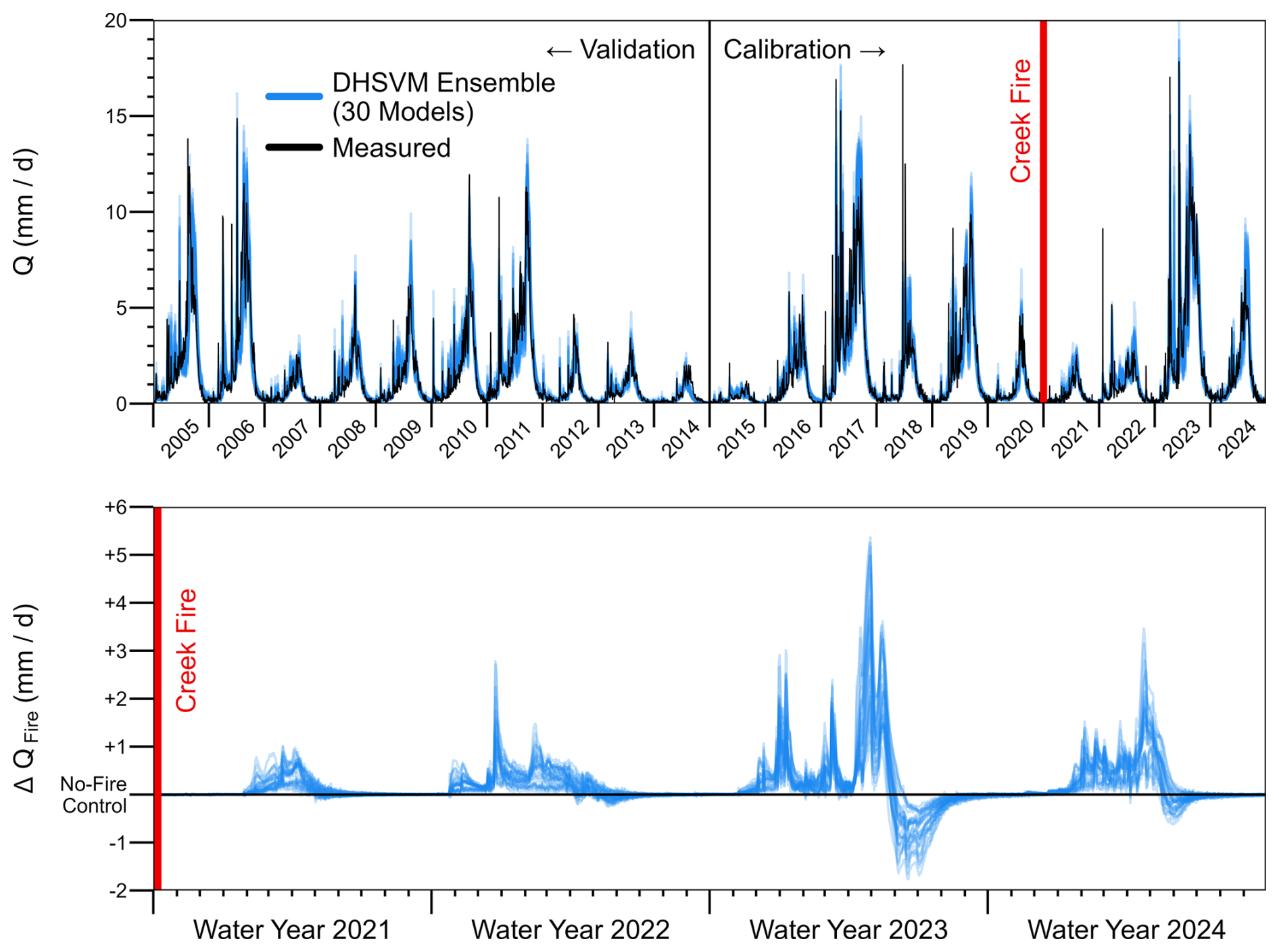
Figure 3 Modeled and measured daily streamflow hydrographs (top panel) and streamflow differences between fire-aware and no-fire control simulations (bottom panel). Both panels show results from 30 calibrated “behavioral” parameter sets (Sect. 2.2).

We constrain the empirical model using pre-fire data and compare its post-fire predictions with measured post-fire streamflow. Meteorological data required for Eq. (3) are aggregated from the same gridMET data used for DHSVM (Abatzoglou, 2013) over water years 1980–2020. As for Eq. (2), we generate 1000 Bayesian samples of the empirical model parameters (c₀, c₁, c₂, and σ) using Hamiltonian Monte Carlo (Stan Development Team, 2023). The empirical model achieves R² = 0.91 for annual variations in runoff efficiency across the 41 year fitting period. By sampling the model's posterior predictive distribution using meteorological data from 2021–2024, we generate 1000 counterfactual estimates of annual streamflow in each of the post-fire years. The difference between measured post-fire streamflow and predicted streamflow from the stationary statistical model provides an estimate of the streamflow change attributable to disturbance.

3 Results

The behavioral ensemble of 30 calibrated DHSVM parameter sets all reproduce observed streamflow hydrographs with a close match to peak flow and low flow magnitudes, interannual variability, and seasonal timing (Table 2, Fig. 3). Daily NSE values for the 2015–2024 calibration period vary between 0.80 and 0.89 among the different parameter sets (logNSE 0.80 to 0.85), with similar statistics on the 2005–2014 validation period (NSE 0.76–0.88, logNSE 0.80–0.87). All behavioral parameter sets also achieve NSE of 0.80 to 0.89 and log-scale NSE of 0.76 to 0.84 considering just the four years after the Creek Fire, which is considered satisfactory because the model skill is similar on pre- and post-fire periods. Additionally, the post-fire daily NSE of at least 0.80 achieved by all behavioral DHSVM parameter sets is substantially higher than the post-fire daily NSE of −0.13 to 0.60 achieved by a different distributed hydrological model (with dynamic vegetation and other fire-aware updates) after a megafire in other Sierra Nevada sub-watersheds (Abolafia-Rosenzweig et al., 2024). Without the vegetation map updates, the behavioral ensemble performs significantly worse on the post-fire period, but streamflow skill is still reasonably high: the mean NSE is lower by 0.06 in the no-fire control scenario (p < 0.001, Welch one-sample t-test) and the mean logNSE is lower by 0.02 (p < 0.001). Furthermore, the no-fire control scenario yields a mean post-fire bias between −17 % and −9 % (static vegetation systematically underestimates post-fire streamflow), while in dynamic vegetation mode the mean post-fire bias varies between −9 % and +6 % (Fig. S3 in the Supplement). Comparing fire-aware and no-fire counterfactual scenarios, the behavioral ensemble indicates a bulk streamflow increase of +2 to +17 % after the Creek Fire (median +12 %). DHSVM also indicates a shift towards earlier snowmelt runoff after the Creek Fire. Because our post-fire implementation only changes the vegetation maps (no change to modeled soil or snow albedo), the prediction of earlier snowmelt runoff is primarily a result of increased energy reaching the snowpack due to reduced canopy shading. This snowmelt timing effect is most noticeable in the 2023 water year, which was a year with extremely high snow accumulation (Marshall et al., 2024).

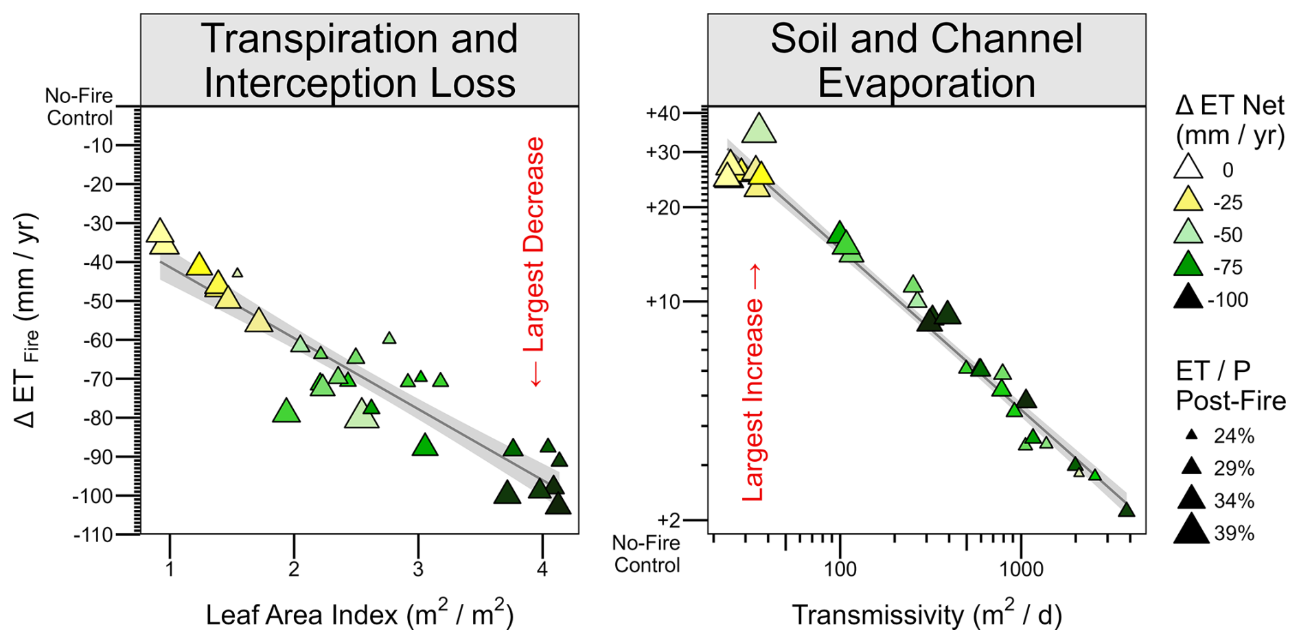
Figure 4 Difference in ET fluxes between fire-aware and no-fire control simulations visualized relative to model parameter uncertainty. Each point represents a single behavioral parameter set (N=30) with all values spatially averaged within the watershed. The area-average leaf area index (LAI) is aggregated within the pre-fire forested area from maps of tree-scale LAI and grid-scale fractional cover (both of which are calibrated, see Table 1), and the area-average transmissivity is aggregated from maps of soil depth, conductivity, and exponential decrease using the DHSVM transmissivity equations (all three of which are also calibrated, see Table 1). Trend lines indicate the least-squares fit and 90 % confidence interval of the best-fit linear estimator.

Uncertainty in the streamflow response to disturbance is large relative to the size of the effect, even after a megafire. The difference in total post-fire streamflow volume between fire-aware and no-fire control scenarios has a coefficient of variation of 41 %. Some parameter sets predict up to a 650 % larger annual streamflow response than other parameter sets (inter-model range of +13 to +97 mm yr⁻¹). Relative uncertainty is higher in dry years, with the simulated streamflow response in 2021 varying between +3 and +47 mm yr⁻¹ across different parameter sets (1400 % range). The predicted streamflow change after the Creek Fire is on the same order of magnitude as stochastic error in the annual water balance (Fig. S3), which intuitively explains why the disturbance response remains uncertain despite direct calibration of pre- and post-fire streamflow (Fig. 3).

Uncertainty in the post-fire streamflow response is linked to equifinality in modeled water balance fluxes (Figs. 1 and 4). To qualify as “behavioral,” parameter sets must satisfactorily estimate the annual water balance (MAPE < 10 %), but the model can achieve this in different ways. Some parameter combinations suggest that transpiration and interception loss from vegetation accounts for up to 95 % of total pre-fire ET, while others suggest a vegetation contribution as low as 77 %, with the balance contributed by evaporation from abiotic surfaces (stream channels and soil, including rock above treeline). Relatively dense initial forests (high area-average LAI) are associated with large decreases in post-fire transpiration and interception loss (Pearson r = −0.92, p < 0.01). Low transmissivity is associated with increases in post-fire soil evaporation and channel evaporation (r = −0.99, p < 0.01, both variables log-transformed).

Compensating errors in equifinal parameter sets can produce compounding discrepancies after disturbance. Not only do some parameter sets indicate much larger changes in individual fluxes, those with the smallest reductions in vegetation ET also exhibit the largest fractional compensation (up to 76 %) from increased abiotic evaporation (r = 0.71, 0.01). A similar compensation between modeled overstory and understory ET components is illustrated by Boardman et al. (2025). Low calibrated transmissivity implies slower groundwater recharge and shallower flowpaths, contributing to higher soil evaporation, which compensates for low vegetation ET. These parameter sets are primed for large increases in evaporation when soil moisture increases in de-forested areas after fire. Consequentially, there is a negative correlation (r = −0.93, p < 0.01) between the fraction of pre-fire ET contributed by abiotic evaporation and the magnitude of the post-fire net ET reduction.

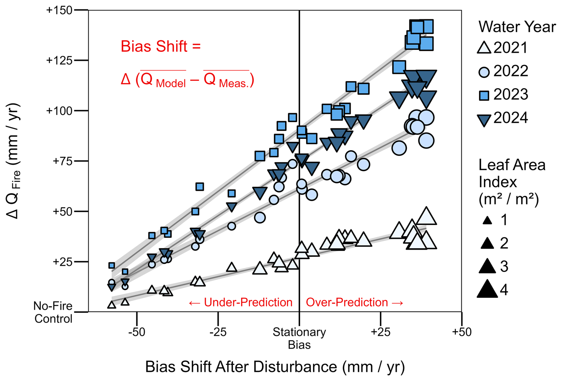
Figure 5 Annual post-fire streamflow change visualized relative to the mean bias shift after disturbance for all 30 parameter sets. Parameter sets with a shift towards overestimation predict a relatively large streamflow response to disturbance, and vice versa. Parameter sets with near-stationary bias are assumed to give the most accurate estimate of changes due to disturbance. Trend lines indicate the least-squares fit and 90 % confidence interval of the best-fit linear estimator, distinct from the analogous Bayesian regression in Eq. (2), which also propagates parameter uncertainty.

Evaluating the model bias shift (Eq. 1) can help escape this morass of uncertainty. Across the 30-member behavioral ensemble, there is a strong correlation (r = 0.96–0.99 depending on year, p < 0.01) between the mean streamflow bias shift after disturbance and the annual streamflow change attributable to fire (Fig. 5). Lines in Fig. 5 correspond to Eq. (2), and the horizontal axis is defined by Eq. (1). Bayesian sampling of a linear model conditioned on zero bias shift yields an estimate of the uncertainty in the vertical intercept (Sect. 2.4), which is the predicted streamflow change of models with stationary bias. Comparing the annual streamflow errors of models with positive or negative bias shift (Fig. S3), we note that the positive-shift models tend to have more-positive errors on the pre-fire period compared to negative-shift models, but this stratification reverses after the Creek Fire. This reversal of model over- and under-prediction after disturbance is consistent with our conceptual model in Fig. 1. Additionally, as shown by the shape-size in Fig. 5, the models with the largest over-prediction have anomalously high overstory LAI, and vice versa, which is similarly consistent with the conceptualization of ET_Tree and ET_Other equifinality in Fig. 1.

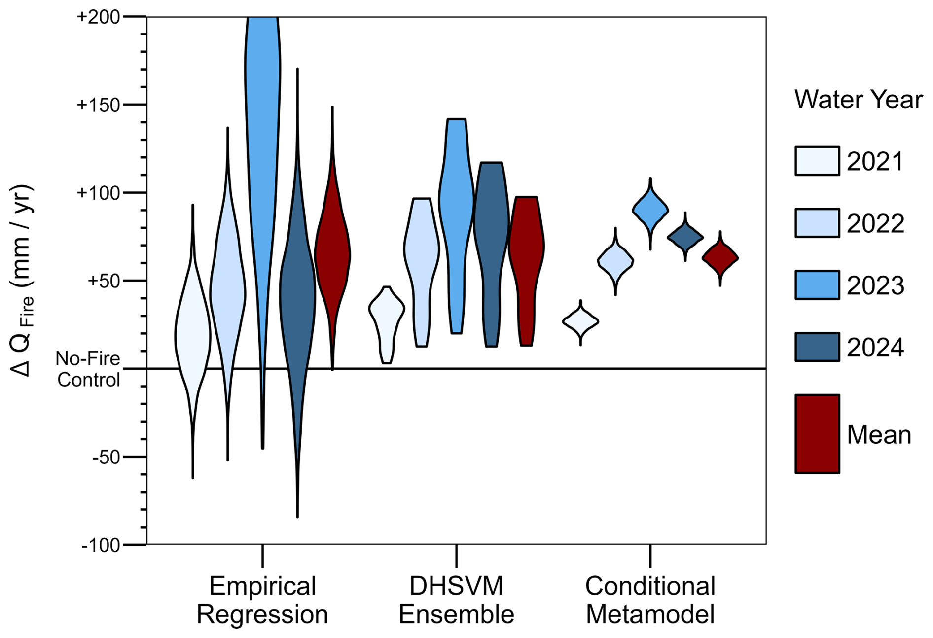
Figure 6 Uncertainty distributions for the annual post-fire streamflow change relative to a control scenario with no fire. Empirical regression results are estimated by comparing post-fire measurements with 1000 random samples of a pre-fire multi-linear regression model (Eq. 3). The DHSVM ensemble represents the difference between fire-aware and no-fire control simulations using 30 different calibrated parameter sets. The conditional metamodel predicts the DHSVM response subject to the requirement of stationary bias using 1000 random samples of the Bayesian regression in Eq. (2). (Note that the vertical axis is truncated at +200 mm yr⁻¹ for increased visibility of most results.)

Eight parameter sets result in near-stationary bias (shift less than ± 10 mm yr⁻¹). This eight-member “stationary sub-ensemble” demonstrates how considering bias shift after disturbance can reduce equifinality. Compared to 10⁴ alternative sub-ensembles of eight parameter sets each randomly selected from the 30-member ensemble, the stationary sub-ensemble has significantly reduced uncertainty in LAI (p < 0.01) and transmissivity (p < 0.02), calculated from the cumulative distribution function for the fractional uncertainty reduction of all 10⁴ sub-ensembles. This uncertainty reduction associated with the stationary sub-ensemble is 72 % larger for LAI and 285 % larger for log-transformed transmissivity compared to the median uncertainty reduction of same-sized sub-ensembles selected randomly. The stationary sub-ensemble has mean 2011-era LAI between 1.9–2.8 m² m⁻², which is 74 % less uncertainty compared to the full behavioral ensemble range of 0.9–4.1 m² m⁻² (Fig. 5). Analogously, the stationary sub-ensemble has 50 % less uncertainty in log-transformed mean transmissivity despite order-of-magnitude residual uncertainty (108–1378 m² d⁻¹). Meteorological uncertainty remains mostly unchanged in the stationary sub-ensemble, with 3.7 °C and 15 % uncertainties in temperature and precipitation biases, respectively, compared to 4.4 °C and 15 % for the behavioral ensemble (no significant change relative to random sub-ensemble selection). This leads to similar uncertainty in the stationary sub-ensemble's post-fire evaporative index ($\text{ET}/P$) compared to the full ensemble (25 %–34 % vs. 24 %–39 %, respectively). Among all 14 calibrated parameters (Table 1), only the melt-season albedo decay rate has a statistically significant difference in the mean (p < 0.05, Welch two-sample t-test) between the stationary sub-ensemble and the full 30-member ensemble. Instead, most of the equifinality reduction arises from shrinking the uncertainty of the parameter distributions rather than changing their mean (Fig. S4) and/or from constraining multi-dimensional parameter interactions (Fig. S1). The 30-member behavioral ensemble has residual meteorological uncertainty ranging from −11 % to +4 % precipitation biases and −3.4 to +1.0 °C temperature biases. Considering only the 8-member stationary sub-ensemble, the precipitation bias uncertainty remains the same (−11 % to +4 %) and the temperature bias uncertainty decreases slightly to a range of −3.1 to +0.3 °C. Although these calibrated meteorological biases are substantially smaller than our ± 25 % calibration range (Table 1), the precipitation uncertainty remains roughly the same magnitude as the post-fire streamflow change, highlighting the potential confounding impact of forcing data on post-disturbance change-detection studies.

Compared to the full behavioral ensemble, the stationary sub-ensemble has slightly sub-optimal hydrograph fit (NSE 0.80–0.85 vs. 0.89 max), but better SWE volume error compared to the highest-NSE parameter set (MAPE of 18 %–27 % across 30 ASO surveys vs. 32 % for the highest-NSE parameter set). The stationary sub-ensemble has statistically lower (worse) mean NSE values compared to the 30-member ensemble (p < 0.05) and approaches the threshold for significantly lower (better) mean SWE volume percent error (p = 0.055). The > 95th-percentile peak flow RMSE is also significantly worse (p < 0.05) for the stationary sub-ensemble. Differences in log-scale NSE and annual or April–July water yield error are not statistically significant. The improvement in snow skill despite a slight worsening of streamflow skill (Fig. S5 in the Supplement) may arise from overfitting during calibration, which leads to a tradeoff between enhanced model physical fidelity (represented by the near-zero bias shift and better snow performance of the stationary sub-ensemble) and minor degradation in the streamflow performance metrics.

Empirical regression and process-based simulations both suggest an increase in streamflow after the Creek Fire, albeit with different uncertainty ranges (Fig. 6). An empirical model (Eq. 3) fit to pre-fire data predicts relatively less post-fire streamflow than observed, implying a total streamflow increase of +12 % with a 90 % credible interval of +5 % to +18 % assuming that each year's error distribution is independent. (The 90% credible interval represents the 5^th-95^th percentiles.) Although the 4 year total streamflow increase is significant at p < 0.01, for individual post-fire years we cannot reject the null hypothesis (no change after disturbance) at the p < 0.01 level, and we cannot even reject the no-change hypothesis at the p < 0.1 level in 2021 or 2024. Compared to the pure statistical model based on the same meteorological data, our process-based modeling approach yields remarkably similar uncertainty. All 30 behavioral DHSVM parameter sets indicate at least some streamflow increase in each post-fire year, with a similar mean increase of +12 % and a marginally wider 90 % range of +3 % to +17 % across the ensemble. Although the 90 % uncertainty ranges are similar between DHSVM and the empirical regression, all of the DHSVM parameter sets show at least some increase. Additionally, within individual years, the DHSVM uncertainty can be much lower (e.g., in 2023, the DHSVM 90 % range is +2 % to +11 %, while the empirical regression 90 % credible interval is +3 % to +23 %). The uncertainty of the empirical model benefits from considering all four years simultaneously because the empirical model assumes that each year's fire effect is independent, while different DHSVM parameter sets are systematically biased high or low across all post-fire years.

Compared to pure statistical or pure process-based approaches, a statistical metamodel trained on DHSVM results and conditioned on bias stationarity can drastically reduce uncertainty. Using 1000 random samples of the metamodel (Eq. 2), we find a +11 % increase in total post-fire streamflow with a 90 % credible interval of +10 % to +12 %. The mean streamflow response is 14 standard deviations above zero, confidently rejecting the no-change hypothesis. Moreover, interannual variability in the conditional streamflow response is separable between all pairs of years at the p < 0.01 level. In contrast, raw DHSVM simulations of the streamflow response in 2022, 2023, and 2024 are not mutually separable at the p < 0.05 level. Comparing 90 % credible intervals, the conditional approach reduces uncertainty in the total post-fire streamflow change by 80 % compared to the empirical regression and 82 % compared to the behavioral DHSVM ensemble. Of course we cannot know precisely what the true streamflow would have been without a fire, so some uncertainty must always remain, but our metamodel results suggest that we can substantially reduce this uncertainty by fusing process-based and statistical approaches.

The independent pre-fire calibration (end of Sect. 2.2) yields similar predictions of the post-fire streamflow change (Fig. S7 in the Supplement). When applied to behavioral parameter sets from the pre-fire calibration, the conditional metamodel predicts a 90 % credible interval of +9 % to +12 % for the total post-fire streamflow change, which is remarkably close to the independent estimate of +10 % to +12 % using the cross-fire (2015–2024) calibration. The conditional metamodel based on the pre-fire calibration reduces uncertainty in the total post-fire streamflow (90 % confidence interval) by 82 % compared to the empirical regression and 74 % compared to the pre-fire behavioral DHSVM ensemble, which is again similar to the analogous 80 % and 82 % reductions (respectively) achieved by the cross-fire calibration metamodel. Regardless of whether DHSVM is calibrated pre- and post-fire, or only pre-fire, the conditional metamodel provides consistent predictions of the additional streamflow attributable to the Creek Fire (ΔQ_Fire).

4 Discussion

Hydrological models must account for forest fires and other environmental disturbances to provide robust predictions for water resource management, risk assessment, and operational planning. In 2021, the first year after the Creek Fire, our hybrid modeling approach estimates that the additional streamflow attributable to forest disturbance provided 0.11 ± 0.03 km³ (92 000 ac−ft.) of extra water to Millerton Lake (a major regional reservoir, Fig. 2), which is 18 % ± 4 % of the total water yield in a year where drought conditions caused curtailment of downstream water rights (California DWR, 2021). In the wet 2023 water year, extra streamflow attributable to the fire totaled ∼ 0.38 ± 0.04 km³ (310 000 ac−ft., 7 % of total water yield), equivalent to an extra 60 % ± 7 % of the reservoir storage capacity in a year with widespread flooding (California DWR, 2023). (All uncertainty ranges indicate the 90 % credible interval.) These examples illustrate the potential for landscape-scale forest disturbance to enhance water resources and/or exacerbate water risks (e.g., Boardman et al., 2025). Accurately representing disturbance and accounting for other sources of nonstationarity should be a priority of ecohydrological modeling.

Our results suggest that equifinality demands thoughtful consideration in hydrological model-based studies of disturbance. At the same time, studies investigating disturbance have a unique and underutilized opportunity to reduce model equifinality. Much of the spread in the DHSVM ensemble (Fig. 6) could be eliminated by reducing the number of calibrated parameters or narrowing their prior range (Table 1). However, in typical landscape-scale simulations, we do not know the “correct” parameter values. For example, there is considerable uncertainty in vegetation properties derived from satellite imagery (Garrigues et al., 2008; Tang et al., 2019) or extrapolated from sparse field data (Meyer et al., 2016). Moreover, in modeling applications, “effective” parameters may subsume additional sources of structural or data uncertainty (Dolman and Blyth, 1997; Vázquez, 2003; Were et al., 2007), and some quasi-empirical parameters (e.g., grid-scale hydraulic conductivity) do not have single “correct” values (Beven, 1993). In our current study, we choose to treat the combination of model and forcing data as a single inferential system, so uncertainty in hydrological parameters is not independent from meteorological biases. This unified approach is useful for our goal of simultaneously constraining multiple sources of uncertainty in the post-fire streamflow change, but other studies may choose to use the same meteorological assumptions across all models to more tightly constrain and explore within-model dynamics. Uncertainty in vegetation properties like LAI can produce significantly different streamflow predictions (e.g., Bart et al., 2016 and Fig. 5 of this study), and latent uncertainty could cause systematic biases (Fig. 4). Furthermore, even if vegetation properties could be tightly constrained, introducing parameter variability into model experiments can reveal compensating ecohydrological processes (Figs. 1 and 4), counterintuitively leading to higher confidence in the statistical metamodel by providing datapoints for regression in Eq. (2). Nevertheless, reducing model parameter uncertainty is generally desirable when justified, and our results show that a sub-ensemble of parameter sets with near-stationary bias after disturbance can significantly reduce uncertainty in LAI (p < 0.01) and transmissivity (p < 0.02).

Using process-based models for post-disturbance predictions based on traditional streamflow calibration metrics can be dangerously misleading. Describing model performance with simple goodness-of-fit metrics (e.g., NSE) is problematic in general due to sampling uncertainty and other issues (Clark et al., 2021), but these metrics remain ubiquitous in modeling studies (including this one) due to their ease of application and simplicity of interpretation. Although these metrics are useful for loosely identifying an initial ensemble of behavioral models, our results provide a clear example of the pitfalls in blindly trusting NSE-based (or similar) calibration strategies. In particular, the four models with the highest daily NSE (0.88–0.89) have anomalously small disturbance effects, and the parameter set with the absolute highest NSE underestimates the post-fire streamflow change by 79 % relative to the metamodel mean (Fig. S6 in the Supplement). These outlying parameter sets are presumably compensating for unknown deficiencies in the model structure and/or forcing data, leading the model to get a slightly higher NSE for what are apparently the wrong reasons. These undesirable and yet numerically optimal solutions are endemic to high-dimensional optimization problems, an issue known as “reward hacking” (Amodei et al., 2016). Although log-transformed NSE appears less vulnerable to reward hacking (Fig. S6), the parameter set with the absolute highest logNSE still underestimates the metamodel-based mean streamflow change by 58 %. It is noteworthy that our ultimate model evaluation metric (bias shift, Fig. 5) is not included in the calibration. If this metric were directly calibrated, it might be susceptible to reward hacking, leading to unreliable inference in Eq. (2).

With care, process-based models can remain powerful tools for hydrological investigation. Despite a recent focus on machine learning approaches to hydrological prediction (Ardabili et al., 2020; Xu and Liang, 2021), purely empirical methods are limited by the amount of available data, the ability to assign clear process attribution, and the potentially ambiguous interpretation of nonstationarity (Slater et al., 2021). In the years immediately after a large forest disturbance (e.g., megafire), water managers may require rapid estimates of the potential hydrological impacts without the luxury of waiting for more data to accrue. Counterfactual model simulations can help isolate disturbance effects from stochastic weather and other variability, but it is notoriously challenging to quantify the uncertainty of distributed process-based models. Direct uncertainty estimation based on subjective likelihood metrics (e.g., GLUE, Beven and Binley, 1992) is statistically unjustified (Mantovan and Todini, 2006; Stedinger et al., 2008). Nevertheless, by using a subjective sample of models to constrain sensitivity (Fig. 5), we can perform classical Bayesian inference (Eq. 2) to sample the relationship between an unknown outcome (e.g., the streamflow response to fire) and an observational constraint (e.g., bias stationarity). This framework overcomes the statistical limitations of process-based models by treating the results from equifinal parameter sets as data points that constrain a statistical metamodel (Eq. 2), which should be transferable to other disturbance studies. Moreover, the statistical metamodel provides an 82 % uncertainty reduction compared to the raw DHSVM ensemble with just four years of post-fire streamflow data in a single watershed. The consistency of the metamodel results between two independent calibrations (pre-fire and cross-fire) suggests that our framework is robust to subjective calibration decisions and random temporal variability, strengthening confidence in the results. Further calibration tests in other watersheds could inform a transferrable understanding of equifinality that might help constrain the post-fire streamflow response with fewer years of post-fire data, and could even help constrain predictions for possible future disturbances before they happen.

Our findings suggest a generally applicable conceptual framework for hydrological model simulations of many types of change beyond just environmental disturbance. In brief, it is important to ensure that our models are stationary with respect to the variability they are used to investigate. For our present study of the streamflow response to a forest fire, the model should have stationary bias across pre- and post-fire periods. For a study on climate warming effects, modelers could test the stationarity of model biases in warmer or cooler years or locations. For a drought study, model bias stationarity could be evaluated between wet and dry periods. Many analogous examples are easily imagined. We anticipate that testing bias stationarity across different types of change can help reduce both equifinality and uncertainty, as shown here.

5 Conclusion

In light of our results from this test application, we offer some general recommendations for process-based simulations of environmental disturbance in a hydrological context.

• Parameter uncertainty extends beyond the subsurface. We suggest calibrating or at least testing the sensitivity of parameters controlling the partitioning of ET fluxes (e.g., overstory/understory transpiration, interception loss, soil evaporation, etc.). Parameter interactions with meteorological uncertainty should also be considered and potentially propagated during calibration, especially when high-precision basin-scale forcing data are unavailable.

• Nonstationary error metrics (e.g., positive or negative bias shift) can indicate a failure to adequately represent change. Rejecting parameter sets with a bias shift after forest disturbance (or with respect to some other change) can help reduce equifinality and thus also reduce uncertainty in modeled hydrological responses to disturbance.

• Modelers should beware of “reward hacking” (i.e., overfitting) during calibration, particularly when applying powerful optimization algorithms to high-dimensional search spaces. In this study, selecting the highest-NSE parameter sets would lead to a 79 % underestimation of the streamflow response to disturbance relative to the mean value of the conditional metamodel (analogous 58 % underestimation using the highest logNSE).

• We caution against direct derivation of uncertainty ranges from subjective parameter ensembles, as this could lead to unnecessarily high uncertainty with poor statistical justification (Fig. 5). Instead, model results can inform a statistical metamodel conditioned on observation-based metrics related to stationarity (e.g., bias shift), enabling the derivation of uncertainty from conditional statistics (Eq. 2). The statistical metamodel structure will necessarily depend on the study objectives, but the principle is generally applicable to other models and types of environmental change.