Error-correction across gauged and ungauged locations: A data assimilation-inspired approach to post-processing river discharge forecasts

Forecasting river discharge is essential for disaster risk reduction and water resource management, but forecasts of the future river state often contain errors. Post-processing reduces forecast errors but is usually only applied at the locations of river gauges, leaving the majority of the river network uncorrected. Here, we present a data-assimilation-inspired method for error-correcting ensemble simulations across gauged and ungauged locations in a post-processing step. Our new method employs state augmentation within the framework of the Local Ensemble Transform Kalman Filter (LETKF). Using the LETKF, an error vector representing the forecast residual is estimated for each ensemble member. The LETKF uses ensemble error covariances to spread observational information from gauged to ungauged locations in a dynamic and computationally efficient manner. To improve the efficiency of the LETKF we define new localisation, covariance inflation, and initial ensemble generation techniques that can be easily transferred between modelling systems and river catchments. We implement and evaluate our new error-correction method for the entire Rhine-Meuse catchment using forecasts from the Copernicus Emergency Management Service's European Flood Awareness System (EFAS). The resulting river discharge ensembles are error-corrected at every grid box but remain spatially and temporally consistent. A spatial cross-validation strategy is used to assess the ability of the method to spread the correction along the river network to ungauged locations. The skill of the ensemble mean is improved at almost all locations including stations both up- and downstream of the assimilated observations. Whilst the ensemble spread is improved at short lead-times, at longer lead-times the ensemble spread is too large leading to an underconfident ensemble. In summary, our method successfully propagates error information along the river network, enabling error correction at ungauged locations. This technique can be used for improved post-event analysis and can be developed further to post-process operational forecasts providing more accurate knowledge about the future states of rivers.

1 Introduction

River discharge forecasts are essential tools for taking effective preparatory actions for disaster mitigation and water resource planning (UNDRR, 2015). However, despite the increased sophistication of forecasting systems over the past few decades, river discharge forecasts still contain uncertainty (Boelee et al., 2019). The uncertainty is introduced at several stages of the forecasting system including the meteorological forcings, the initial conditions, and the hydrological model structure and parameters (Valdez et al., 2022). Ensemble river discharge forecasts typically aim to account for the meteorological uncertainty by forcing a hydrological model with many meteorological forcings (Cloke and Pappenberger, 2009; Wu et al., 2020). However, ensemble forecasts can still contain biases and errors in the representation of uncertainty. Different methods for correcting these errors have been developed including pre-processing of the meteorological forcings, calibration of the hydrological model, improving the initial conditions using data assimilation, and post-processing of the river discharge forecast (Bourdin et al., 2012). Of these approaches post-processing is often considered the most computationally efficient and its ability to correct for multiple sources of errors simultaneously is appealing.

In meteorological forecasting, post-processing at non-observed locations is common (see Vannitsem et al., 2021). However, hydrological forecasting requires consideration of the spatial heterogeneity introduced by the river network (e.g., Li et al., 2017; Woldemeskel et al., 2018; Ye et al., 2014; Xu et al., 2019; Liu et al., 2022; Lee and Ahn, 2024) making hydrological post-processing at ungauged locations a difficult challenge. The global river gauge network is sparse (Krabbenhoft et al., 2022), and even in regions where gauges exist, river discharge data are often not widely shared (Lavers et al., 2019; Hannah et al., 2011). Therefore, the development of post-processing techniques for ungauged locations is essential. However, current techniques are generally too computationally expensive for operational river flow forecasting applications (Emerton et al., 2016). For example, defining a joint distribution between the river discharge at multiple locations would allow forecasts to be conditioned on observations available at specific locations (Engeland and Steinsland, 2014). However, for large-scale distributed systems and multiple lead-times the size of the joint distribution quickly becomes too large. Alternatively, error-correction can be performed at a gauged location and the results interpolated to ungauged locations. One such method used to interpolate error-correction parameters is top-kriging (Pugliese et al., 2018; Skøien et al., 2021). Top-kriging takes into account the river network but the relationship between errors at different locations is assumed static regardless of the hydrometeorological situation (Skøien et al., 2016, 2006). Another option is to use a river routing model to propagate error-corrected river discharge forecasts between gauged locations (Bennett et al., 2022). Whilst this approach maintains spatial consistency between locations, the additional run of the model could be computationally expensive for an operational application.

The aim of this paper is to present and evaluate a novel technique for spreading observation information from gauged to ungauged locations in a computationally efficient and temporally varying manner. The new method is based on data assimilation techniques. Data assimilation is a mathematical technique that combines modelled predictions and observations to produce a better estimate of the true state of the river (Nichols, 2003, 2009). Data assimilation is often used to improve the initial conditions of forecasts (Valdez et al., 2022). However, in this paper we modify the techniques to apply them in a post-processing environment such that additional, computationally expensive, executions of the hydrological model are not required. The error correction method proposed in this study is based on state augmentation (Dee, 2005) and the Local Ensemble Transform Kalman Filter (LETKF, Hunt et al., 2007). State augmentation is a technique that allows the estimation of the state and parameters/biases of a system simultaneously, and is often used for online bias-estimation in data assimilation (Ridler et al., 2018; Gharamti and Hoteit, 2014; Smith et al., 2013, 2009; Martin et al., 2002). The LETKF is part of the Kalman filter family of methods and uses an ensemble of model states to estimate the state error covariances. Due to their computational efficiency and ability to handle non-linear dynamics without an adjoint model, ensemble Kalman filters are common data assimilation methods in hydrological research (Rouzies et al., 2024; Li et al., 2023; Mason et al., 2020; Ridler et al., 2018; Khaki et al., 2017; Xie and Zhang, 2010; Clark et al., 2008).

Whilst many studies have shown the benefits of data assimilation for hydrological forecasting (Tanguy et al., 2025; Valdez et al., 2022; Piazzi et al., 2021), the process is rare in operational systems (Pechlivanidis et al., 2025), particularly in large-scale systems (Wu et al., 2020). This limited uptake is partly due to data latency issues (WMO, 2024), time constraints, and the potential impact on the interpretation of the forecasts (e.g., thresholds based on model climatology may no longer be consistent; Emerton et al., 2016). Additionally, the benefit of data assimilation at longer lead-times is uncertain (e.g., Valdez et al., 2022). In this paper, we leverage key advantages of data assimilation – such as the ability to propagate observational information to ungauged locations – within a post-processing framework that is more readily integrated into operational systems.

The proposed method aims to improve the skill of the ensemble mean and the reliability of the ensemble spread by adjusting each ensemble member, as will be discussed in more detail in Sect. 2. However, it is equally, if not more, important that the ensembles are spatially and temporally consistent in order to aid with decision making (Bennett et al., 2022). This is particularly important for large scale systems that provide forecasts across administrative boundaries, such as the Copernicus Emergency Management Service’s (CEMS) European Flood Awareness System (EFAS) used in this study (Matthews et al., 2025). The specific research questions to be addressed in this study are therefore,

1. Can data assimilation techniques be used in a post-processing environment to propagate observation information to ungauged locations?

2. Are the resulting ensemble predictions of river discharge more skillful than the raw ensemble?

This paper is organised as follows. In Sect. 2 we define the errors which we aim to correct and introduce some terminology and notation. In Sect. 3 we describe the data assimilation techniques used within this study. In Sect. 4 we outline the proposed error-correction method and detail how the ensemble is corrected. Section 5 provides some additional components of the method that improve the efficacy of the method but which can be adjusted to suit the data availability of any system and/or domain. Section 6 outlines the strategy used to evaluate the efficacy of the proposed method. Section 7 presents the results, first investigating the impact of assimilating the observations, and then assessing the skill of the error-corrected ensembles. In Sect. 8 we discuss key features of the proposed method and their impact on the error-corrected ensembles. In Sect. 9 we conclude that the proposed method successfully improves the skill of the ensemble mean, and highlight priorities for future developments.

Please note that throughout the paper “hindcast ensemble” refers to the ensembles of river discharge that we are error-correcting. In this paper, these ensembles are past operational EFAS forecasts (see Sect. 6.1). However, when we perform the error-correction we use observations that are available within the forecast (hindcast) period. Observations are not available during the forecast period in an operational system, since these timesteps are in the future. Therefore, we refer to these river discharge ensembles as hindcasts to indicate that the ensembles are not valid forecasts.

2 Ensemble error-correction framework

Here, we define the errors which we aim to correct and provide some notation that is used throughout the paper. Where possible we follow the standard data assimilation notation provided in Ide et al. (1997). Let the true state of the system at time k be defined as ${\mathit{x}}_k^{\mathrm{true}}\in {\mathbb{R}}^n$, where each element represents the true river discharge in one of the n grid boxes in the domain of interest. Hydrological forecasts generally estimate the true state of the system using a modelled state, denoted x_k, where the lack of superscript “true” indicates it is a modelled estimate. In this study, the hydrological ensemble forecasts consist of N potential realizations of future river discharge, referred to as ensemble members. We define the ensemble river discharge hindcasts as

$$\begin{array}{}\text{(1)}& \left\{{\mathit{x}}_k:{\mathit{x}}_k^{\left(i\right)},\text{ for }i=\mathrm{1},\mathrm{2},\mathrm{\dots },N\text{ and }k=\mathrm{0},\mathrm{1},\mathrm{\dots },L\right\}.\end{array}$$

where the superscript (i) indicates the ith member of the ensemble, N is the ensemble size, the timestep k refers to the lead-time of the hindcast, and L is the maximum lead-time. The ensemble mean is defined as

$$\begin{array}{}\text{(2)}& {\stackrel{\mathrm{‾}}{\mathit{x}}}_k={\displaystyle \frac{\mathrm{1}}{N}}\sum _{i=\mathrm{1}}^N{\mathit{x}}_k^{\left(i\right)}\in {\mathbb{R}}^n.\end{array}$$

The ensemble perturbation matrix is defined as

$$\begin{array}{}\text{(3)}& {\mathbf{X}}_k=\left(\begin{array}{cccc}{\mathit{x}}_k^{\left(\mathrm{1}\right)}-{\stackrel{\mathrm{‾}}{\mathit{x}}}_k& {\mathit{x}}_k^{\left(\mathrm{2}\right)}-{\stackrel{\mathrm{‾}}{\mathit{x}}}_k& \mathrm{\cdots }& {\mathit{x}}_k^{\left(N\right)}-{\stackrel{\mathrm{‾}}{\mathit{x}}}_k\end{array}\right)\in {\mathbb{R}}^{n\times N}\end{array}$$

where the ith column represents the ith ensemble member's departure from the ensemble mean at lead-time k. The perturbation matrix contains information about the spread of the ensemble and the spatial structure of the deviations of each ensemble member from the mean. From the definition of the perturbation matrix, the ensemble covariance matrix is defined as

$$\begin{array}{}\text{(4)}& {\mathbf{P}}_k={\displaystyle \frac{\mathrm{1}}{N-\mathrm{1}}}{\mathbf{X}}_k{\mathbf{X}}_k^{\mathrm{T}}\in {\mathbb{R}}^{n\times n}.\end{array}$$

where the superscript “T” indicates the matrix transpose.

In this paper, we propose a method to spread an error-correction from gauged locations to every grid box in the domain. The proposed method estimates an additive error vector for each hindcast ensemble member at each timestep. Each element of the error vector represents the error associated with a single grid box in the domain. Collectively, these error vectors form an ensemble defined as,

$$\begin{array}{}\text{(5)}& \left\{{\mathit{b}}_k^{\left(i\right)}\in {\mathbb{R}}^n\text{ for }i=\mathrm{1},\mathrm{2},\mathrm{\dots },N\right\}\end{array}$$

where N is the same ensemble size as the river discharge hindcast, n is the number of grid-boxes in the hindcast domain, and k is the timestep. The error ensemble mean, ${\stackrel{\mathrm{‾}}{\mathit{b}}}_k$, and the ensemble perturbation matrix, B_k, are calculated by substituting ${\mathit{b}}_k^{\left(i\right)}$ in place of ${\mathit{x}}_k^{\left(i\right)}$ in Eqs. (2) and (3), respectively. We assume there is an additive relationship between each hindcast ensemble member and the corresponding error vector such that the ith error-corrected ensemble member, ${\mathit{x}}_k^{\mathrm{new},\left(i\right)}$, is defined as

$$\begin{array}{}\text{(6)}& {\mathit{x}}_k^{\mathrm{new},\left(i\right)}={\mathit{x}}_k^{\left(i\right)}+{\mathit{b}}_k^{\left(i\right)}\in {\mathbb{R}}^n.\end{array}$$

The estimation of the error ensemble at each timestep is described in Sect. 4.

To aid with the estimation of the error vectors, we assume that at each timestep the system is observed at p_k river discharge gauges. We assume the observation vector, ${\mathit{y}}_k\in {\mathbb{R}}^{p_k}$, is related to the true state of the system as

$$\begin{array}{}\text{(7)}& {\mathit{y}}_k={\mathbf{H}}_k\left({\mathit{x}}_k^{\mathrm{true}}\right)+{\mathit{ϵ}}_k\end{array}$$

where ${\mathit{ϵ}}_k\in {\mathbb{R}}^{p_k}$ is a vector of unbiased Gaussian noise with covariance matrix ${\mathbf{R}}_k\in {\mathbb{R}}^{p_k\times p_k}$, and ${\mathbf{H}}_k\in {\mathbb{R}}^{p_k\times n}$ is the linear observation operator. The observation operator maps the variables from the state space to observation space. In this study, the observation operator selects the grid boxes within the modelled drainage network that correspond to the locations of the river gauges.

3 Data Assimilation

As discussed in Sect. 1, the proposed method is based on common data assimilation techniques: state augmentation and the Local Ensemble Transform Kalman Filter (LETKF). In this section, we provide an overview of these techniques and introduce the necessary equations. In Sect. 4, we adapt and apply these methods in a non-standard way due to their application in a post-processing environment.

3.1 State augmentation

State augmentation is a technique used for online bias-correction in data assimilation that allows the simultaneous estimation of the system state and biases. An augmented state is defined by appending the biases to the state vector, allowing both to be updated by the data assimilation method. In this study, the ith member of the augmented ensemble is defined as

$$\begin{array}{}\text{(8)}& {\mathit{w}}_k^{\left(i\right)}=\left(\begin{array}{c}{\mathit{x}}_k^{\left(i\right)}\\ {\mathit{b}}_k^{\left(i\right)}\end{array}\right)\in {\mathbb{R}}^{\mathrm{2}n}.\end{array}$$

where x⁽ⁱ⁾∈ℝⁿ and b⁽ⁱ⁾∈ℝⁿ are the i-th hindcast and error ensemble members, respectively. The augmented ensemble mean and perturbation matrix are given by

$$\begin{array}{}\text{(9)}& {\displaystyle }{\stackrel{\mathrm{‾}}{\mathit{w}}}_k=\left(\begin{array}{c}{\stackrel{\mathrm{‾}}{\mathit{x}}}_k\\ {\stackrel{\mathrm{‾}}{\mathit{b}}}_k\end{array}\right)\in {\mathbb{R}}^{\mathrm{2}n}\text{ and }{\mathbf{W}}_k=\left(\begin{array}{c}{\mathbf{X}}_k\\ {\mathbf{B}}_k\end{array}\right)\in {\mathbb{R}}^{\mathrm{2}n\times N}\end{array}$$

where $\stackrel{\mathrm{‾}}{\mathit{x}}$ and $\stackrel{\mathrm{‾}}{\mathit{b}}$ are the ensemble means of the hindcast and error ensembles, respectively, and X and B are the perturbation matrices of the hindcast and error ensembles, respectively.

In this study, state augmentation is used within an LETKF (described in Sect. 3.2) and it is therefore necessary to define the evolution of the augmented states between timesteps. The evolution of the hindcast and error ensembles determines the evolution of the augmented states. The hindcasts used in this study were generated using the LISFLOOD hydrological model, which is used in the EFAS operational system (Van Der Knijff et al., 2010). As the true evolution of the error vectors at all grid-boxes is unknown, we assume a simple persistence model, such that ${\mathit{b}}_k^{\left(i\right)}={\mathit{b}}_{k-\mathrm{1}}^{\left(i\right)}$. This is a common assumption used in state augmentation (Pauwels et al., 2020; Ridler et al., 2018; Rasmussen et al., 2016; Martin, 2001). Based on the independent evolution of the hindcast and error ensembles, and the additive relationship between their members (Eq. 6), we define the propagation of the augmented ensemble members as

$$\begin{array}{}\text{(10)}& {\mathit{w}}_k^{\left(i\right)}=\left(\begin{array}{cc}{\mathbf{M}}_{k-\mathrm{1}}& {\mathbf{I}}_{k-\mathrm{1}}\\ {\mathbf{0}}_{k-\mathrm{1}}& {\mathbf{I}}_{k-\mathrm{1}}\end{array}\right)\left(\begin{array}{c}{\mathit{x}}_{k-\mathrm{1}}^{\left(i\right)}\\ {\mathit{b}}_{k-\mathrm{1}}^{\left(i\right)}\end{array}\right)=\left(\begin{array}{c}{\mathit{x}}_k^{\left(i\right)}+{\mathit{b}}_{k-\mathrm{1}}^{\left(i\right)}\\ {\mathit{b}}_{k-\mathrm{1}}^{\left(i\right)}\end{array}\right).\end{array}$$

where ${\mathbf{M}}_{k-\mathrm{1}}\in {\mathbb{R}}^{n\times n}$ is a linear evolution operator representing the LISFLOOD hydrological model and ${\mathbf{I}}_{k-\mathrm{1}}\in {\mathbb{R}}^{n\times n}$ is the identity matrix. Since we use precomputed hindcast ensembles the propagation of the hindcast ensemble members requires no additional computation. The full non-linear LISFLOOD hydrological model is also used without the need to define a linear approximation.

3.2 Local Ensemble Transform Kalman Filter (LETKF)

The Local Ensemble Transform Kalman Filter (LETKF; Hunt et al., 2007) updates the mean state and the perturbation matrix of an ensemble by combining the modelled and observed data. As a sequential data assimilation method, the LETKF consists of a propagation step (also known as a forecast step) and an update step (also known as an analysis step) that are cycled. In this method, we use the LETKF to update the ensemble of error vectors at each hindcast timestep for which observations are available. However, we modify the propagation step to use precomputed hindcasts. The propagation step evolves the augmented states forward in time from time k−1 to k, as described in Eq. (10). Rather than evolve the hindcast ensemble explicitly (which would require the hydrological model), we use the precomputed hindcast at timestep k.

The update step of the LETKF calculates the state of the system at timestep k by combining the modelled augmented states and observations. Both data are weighted by their respective uncertainties, represented by their covariance matrices. As the LETKF is a well documented method we only provide the key update equations. For more detailed derivations, we direct the reader to Hunt et al. (2007) and Livings et al. (2008). To apply the LETKF to the augmented ensemble, we create a model-observation ensemble with an ensemble mean, ${\stackrel{\mathrm{‾}}{\mathit{y}}}_k^{\mathit{x}}$, defined as

$$\begin{array}{}\text{(11)}& {\stackrel{\mathrm{‾}}{\mathit{y}}}_k^{\mathit{x}}=\left({\mathbf{H}}_k\mathbf{0}\right){\stackrel{\mathrm{‾}}{\mathit{w}}}_k={\mathbf{H}}_k{\stackrel{\mathrm{‾}}{\mathit{x}}}_k+{\mathbf{H}}_k{\stackrel{\mathrm{‾}}{\mathit{b}}}_{k-\mathrm{1}}\end{array}$$

where ${\mathbf{H}}_k\in {\mathbb{R}}^{p_k\times \mathrm{2}n}$ is the observation operator defined in Eq. (7). The LETKF can then update the augmented ensemble mean, ${\stackrel{\mathrm{‾}}{\mathit{w}}}_k$, such that,

$$\begin{array}{}\text{(12)}& {\stackrel{\mathrm{‾}}{\mathit{w}}}_k^{\mathrm{a}}={\stackrel{\mathrm{‾}}{\mathit{w}}}_k^{\mathrm{f}}+\left(\begin{array}{c}{\mathbf{K}}_{{\mathit{x}}_k}\\ {\mathbf{K}}_{{\mathit{b}}_k}\end{array}\right)({\mathit{y}}_k-{\stackrel{\mathrm{‾}}{\mathit{y}}}_k^{\mathit{x}\mathrm{f}}),\end{array}$$

where the superscripts “f” and “a” indicate the state before and after the update step, respectively; ${\mathbf{K}}_{{\mathit{x}}_k}\in {\mathbb{R}}^{n\times p}$ and ${\mathbf{K}}_{{\mathit{b}}_k}\in {\mathbb{R}}^{n\times p}$ are the components of the Kalman gain matrix acting on the hindcast ensemble and the error ensemble respectively; and y_k∈ℝ^p is the observation vector defined in Eq. (7). The difference between the observations and the model state in observation space (i.e., ${\mathit{y}}_k-{\stackrel{\mathrm{‾}}{\mathit{y}}}_k^{\mathit{x}f}$) is called the innovation vector. The Kalman gain matrix determines the impact of the innovation vector in the update step. The respective uncertainties of the prior modelled state and the observations determine their weight within the LETKF. Large observation uncertainties reduce the Kalman gain, while large uncertainties in the prior state increase the Kalman gain. Both the hindcast and the error components of the Kalman gain are functions of the covariance matrix of the augmented ensemble (see Appendix A; Bell et al., 2004). The covariance matrix describes the state error covariances between grid-boxes allowing the Kalman gain to spread the observation information to ungauged locations. To update the error component specifically, it is the cross-covariances between the error component and the hindcast component that control the spread of the observation information to ungauged locations (see Eq. 9 in Bell et al., 2004). This ability to spread the observational information is key to the error-correction method presented in this study.

The LETKF updates the augmented ensemble perturbation matrix, W_k, such that,

$$\begin{array}{}\text{(13)}& {\mathbf{W}}_k^{\mathrm{a}}={\mathbf{W}}_k^{\mathrm{f}}{\mathbf{T}}_k\end{array}$$

where ${\mathbf{T}}_k\in {\mathbb{R}}^{N\times N}$ is the square root transform matrix (Livings et al., 2008). The square root transform matrix is derived using the Kalman gain matrix which gives the weighting between the modelled state and the observations (Livings et al., 2008). Using an eigenvector decomposition, the square root transform matrix rescales and rotates the ensemble members such that the updated perturbation matrix represents the uncertainty in the updated ensemble mean. The square root transform matrix allows the covariance matrix of the ensemble to be updated without the need for the covariances to be explicitly calculated which can be computationally expensive (Bishop et al., 2001; Hunt et al., 2007). These update equations are used to update the error component only, as will be discussed in Sect. 4.1.

4 Spatially consistent error-correction method for river discharge

In this section, we describe how we use the data assimilation techniques discussed in Sect. 3, to post-process the hindcasts across the domain, including at ungauged locations (Fig. 1). The correction is applied in a post-processing environment, avoiding the need for additional executions of the hydrological model which can be computationally expensive. In Sect. 4.1, we describe how the error ensemble is updated at every timestep. In Sect. 4.2, we describe how the updated error ensemble is used to error-correct the ensemble. Specific experimental design choices are discussed in Sect. 5.

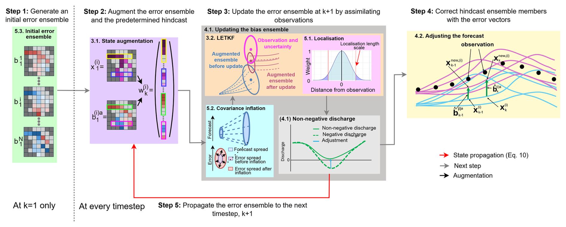
Figure 1 Schematic of the new error-correction method for gauged and ungauged locations. Coloured boxes indicate different components of the method. An initial error ensemble is created for timestep k=1 (green box). Then, the error ensemble is augmented to the hindcast ensemble (purple box). At each timestep the covariance of the augmented ensemble is inflated (cyan box) before being updated using the LETKF, which uses localisation to improve the results of the update (collectively the orange box). The updated error ensemble is adjusted to ensure non-negative discharge values (light grey box) before being used to error-correct the hindcast (yellow box). The non-negative error ensemble is propagated to the next timestep (red arrow). More details are provided for each component in the section indicated in the top left corner of the corresponding box.

4.1 Updating the error ensemble

At each timestep the error ensemble is updated to estimate the optimal set of error vectors to correct the hindcast at that timestep. The update is performed using the LETKF defined in Sect. 3.2. Using the definition of the augmented state in Eq. (8) the update equations for the error ensemble only are,

$$\begin{array}{}\text{(14)}& {\stackrel{\mathrm{‾}}{\mathit{b}}}_k^{\mathrm{a}}={\stackrel{\mathrm{‾}}{\mathit{b}}}_k^{\mathrm{f}}+{\mathbf{K}}_{{\mathit{b}}_k}({\mathit{y}}_k-{\stackrel{\mathrm{‾}}{\mathit{y}}}_k^{\mathit{x}})\end{array}$$

and

$$\begin{array}{}\text{(15)}& {\mathbf{B}}_k^{\mathrm{a}}={\mathbf{B}}_k^{\mathrm{f}}{\mathbf{T}}_k.\end{array}$$

As the hindcast component is not explicitly evolved, we assume that the raw hindcast is a good approximation for the hindcast analysis state if the component were to be updated. This allows the substitution of the precomputed hindcast in place of the propagated state at the next timestep. Thus, the updated mean of the augmented ensemble can be defined as

$$\begin{array}{}\text{(16)}& {\stackrel{\mathrm{‾}}{\mathit{w}}}_k^{\mathrm{a}}=\left(\begin{array}{c}{\stackrel{\mathrm{‾}}{\mathit{x}}}_k\\ {\stackrel{\mathrm{‾}}{\mathit{b}}}_k^{\mathrm{a}}\end{array}\right)\in {\mathbb{R}}^{\mathrm{2}n}.\end{array}$$

where ${\stackrel{\mathrm{‾}}{\mathit{x}}}_k$ is the ensemble mean of the raw hindcast ensemble and ${\stackrel{\mathrm{‾}}{\mathit{b}}}_k^{\mathrm{a}}$ is the updated error ensemble mean (Eq. 14). The perturbation matrix of the updated augmented ensemble follows a similar pattern such that

$$\begin{array}{}\text{(17)}& {\mathbf{W}}_k^{\mathrm{a}}=\left(\begin{array}{c}{\mathbf{X}}_k\\ {\mathbf{B}}_k^{\mathrm{a}}\end{array}\right).\end{array}$$

where X_k is the ensemble perturbation matrix of the raw hindcast ensemble and ${\mathbf{B}}_k^{\mathrm{a}}$ is the updated error ensemble perturbation matrix (Eq. 15). The assumptions made in Eqs. (16) and (17) make our system sub-optimal from a data assimilation perspective but are necessary to avoid rerunning the hydrological model. Importantly, we aim to estimate the error of the precomputed model output at each lead time. Therefore, while the lack of state evolution makes the hindcast component update sub-optimal, the update of the error ensemble remains mathematically consistent. In this study, we provide proof-of-concept that the resulting error ensemble improves the skill of the hindcast (see Sect. 7).

The Kalman filter is not constrained to enforce non-negativity of the analysis state, and therefore, could lead to negative discharge values for some grid boxes if the cross-covariances are incorrectly defined. We enforce non-negativity by further adjusting the error ensemble members after the LETKF update step. For any ensemble member and grid box where the sum of the hindcast discharge and the updated error is negative, we modify the error value so that the total becomes a small positive value, mitigating the potential for instabilities caused by zero-values. This small positive value is sampled from a Gaussian distribution with a mean of zero and a standard deviation equal to 10 % of the standard deviation of the updated error ensemble at the grid-box of interest.

The updated positive-definite augmented states are propagated to the next timestep as defined in Eq. (10). The updated positive-definite augmented states are also used to error-correct the hindcast (Sect. 4.2).

4.2 Adjusting the forecast

After the error component of the augmented state has been updated using Eqs. (14) and (15), and non-negativity has been enforced (Sect. 4.1), the error ensemble members are added to the respective hindcast ensemble members such that

$$\begin{array}{}\text{(18)}& {\mathit{x}}_k^{\mathrm{new},\left(i\right)}={\mathit{x}}_k^{\left(i\right)}+{\widehat{\mathit{b}}}_k^{\left(i\right)\mathrm{a}}\end{array}$$

where ${\mathit{x}}_k^{\mathrm{new},\left(i\right)}$ and ${\mathit{x}}_k^{\left(i\right)}$ are the ith ensemble members of the error-corrected and raw hindcast ensembles, respectively, and ${\widehat{\mathit{b}}}_k^{\left(i\right)a}$ is the error vector associated with the ith error ensemble member where the caret indicates a non-negativity check has been applied. Consequently, the error-corrected hindcast ensemble mean and perturbation matrix are given by

$$\begin{array}{}\text{(19)}& {\stackrel{\mathrm{‾}}{\mathit{x}}}_k^{\mathrm{new}}={\stackrel{\mathrm{‾}}{\mathit{x}}}_k+{\stackrel{\mathrm{‾}}{\widehat{\mathit{b}}}}_k^{\mathrm{a}}\end{array}$$

and

$$\begin{array}{}\text{(20)}& {\mathbf{X}}_k^{\mathrm{new}}={\mathbf{X}}_k+{\widehat{\mathbf{B}}}_k^{\mathrm{a}}.\end{array}$$

This update results in an additive spread correction matrix, Γ_k, with the form

$$\begin{array}{}\text{(21)}& {\mathbf{\Gamma }}_k={\mathbf{X}}_k{\widehat{\mathbf{B}}}_k^{\mathrm{aT}}+{\widehat{\mathbf{B}}}_k^{\mathrm{a}}{\mathbf{X}}_k^{\mathrm{T}}+{\widehat{\mathbf{B}}}_k^{\mathrm{a}}{\widehat{\mathbf{B}}}_k^{\mathrm{aT}}\end{array}$$

where X_k and ${\widehat{\mathbf{B}}}_k^{\mathrm{a}}$ are the perturbation matrices of the raw hindcast and error ensembles, respectively, and the superscript “T” indicates the matrix transpose (Sect. 5.2 in Martin, 2001). Whilst Γ_k can be negative it should be noted that the covariance matrix of the corrected ensemble, ${\mathbf{X}}_k^{\mathrm{new}}{\mathbf{X}}_k^{\mathrm{new},T}$, is positive-definite by definition.

5 Experimental implementation

In Sect. 4 we presented a new method of spreading observation information to ungauged locations in a post-processing environment based on common data assimilation techniques. In this section, we describe three key components of the method – localisation, covariance inflation, and the generation of the initial error ensemble – which are crucial for its performance but can be implemented in various ways.

5.1 Localisation

Localisation is used to reduce the effect of spurious correlations which can arise due to sampling errors caused by the small ensemble size (Hamill et al., 2001; Hunt et al., 2007). The LETKF uses observation localisation which reduces the impact of observations by multiplying the inverse of the observation-error covariance matrix by a localisation matrix, $\mathit{\rho }\in {\mathbb{R}}^{p_k\times p_k}$, such that

$$\begin{array}{}\text{(22)}& {\mathbf{R}}^{-\mathrm{1}}=\mathit{\rho }\circ {\mathbf{R}}_{\mathrm{nl}}^{-\mathrm{1}}\end{array}$$

where $\mathbf{R}\in {\mathbb{R}}^{p_k\times p_k}$ is the localised observation-error covariance matrix used in the LETKF (Sect. 3.2), ${\mathbf{R}}_{\mathrm{nl}}\in {\mathbb{R}}^{p_k\times p_k}$ is the non-localised observation-error covariance matrix, and the symbol ∘ indicates the Schur product (also known as the Hadamard product) which is an element-wise matrix multiplication (Golub and Van Loan, 2013). We assume that R_nl and, by definition, R are diagonal matrices. In this study we use distance-based localisation so the impact of the multiplication described in Eq. (22) is to increase the effective uncertainty of distant observations and thus decrease their impact on the analysis state. The impact of the localisation on the spatial extent of the analysis increments is demonstrated in Sect. 7.1.

The localisation matrix is defined using the Gaspari-Cohn function which has a parameter called the localisation length scale (Appendix B; Gaspari and Cohn, 1999). The Gaspari-Cohn function smoothly decreases the weights assigned to an observation as the distance from the observation location increases, starting from a value of 1 at the observation location and reaching 0 for distances greater than twice the localisation length scale (pink box, Fig. 1). In this study, the distance is calculated along the river network which has been shown to improve the analysis for fluvial applications (García-Pintado et al., 2015; El Gharamti et al., 2021; Khaniya et al., 2022). The distance between a grid-box and the location of an observation is calculated using the local drainage direction map and the channel length of the hydrological model (Choulga et al., 2023). As the distance is defined along the river network, observations cannot impact grid-boxes in a different drainage basin.

Sensitivity experiments conducted during the development of this method found that the optimal length scale varied by location, lead-time, and tuning metric of choice, but overall, the differences were small for length scales from 65 to 786 km (not shown). Therefore, we propose instead for the localisation length scale to be defined as the maximum distance between any grid point and its closest observation. This (1) ensures that all grid boxes are updated in the update step of the LETKF reducing the potential for discontinuities in the analysis state, (2) can adapt to changes in the availability of observations, and (3) can be applied to different domains and hydrological model configurations without requiring a tuning experiment.

5.2 Covariance inflation

Small ensemble sizes can cause underestimation of the ensemble spread, reducing the impact of the observations on the analysis (Furrer and Bengtsson, 2007). Additionally, we assume the error ensemble is constant between timesteps which, while simplifying implementation, could introduce model errors into the ensemble (Evensen et al., 2022). To ameliorate these issues, various covariance inflation techniques are often used (Duc et al., 2020; Scheffler et al., 2022). We implement a heuristic covariance inflation method inspired by the relaxation-to-prior perturbations technique (Zhang et al., 2004; Kotsuki et al., 2017). However, as we are working within a post-processing context, we adapt the method for use with predefined ensembles (i.e., without evolving the inflated perturbations between timesteps).

We blend the prior perturbation matrix at k+1 with an estimated perturbation matrix ${\mathbf{W}}_{k+\mathrm{1}}^{\mathrm{est}}$ similar to the use of a climatological covariance matrix in Valler et al. (2019). The resulting perturbation matrix is given by

$$\begin{array}{}\text{(23)}& {\mathbf{W}}_{k+\mathrm{1}}^{\inf }=(\mathrm{1}-\mathit{\alpha })\left(\begin{array}{cc}{\mathbf{M}}_k& {\mathbf{I}}_k\\ {\mathbf{0}}_k& {\mathbf{I}}_k\end{array}\right){\mathbf{W}}_k^{\mathrm{a}}+\mathit{\alpha }{\mathbf{W}}_{k+\mathrm{1}}^{\mathrm{est}}\end{array}$$

where α is an inflation parameter to be defined (and the definition of the matrices M_k and I_k are given in Sect. 3.1). This blending of matrices introduces both additive and multiplicative inflation. We define ${\mathbf{W}}_{k+\mathrm{1}}^{\mathrm{est}}$ as

$$\begin{array}{}\text{(24)}& {\mathbf{W}}_{k+\mathrm{1}}^{\mathrm{est}}=\left(\begin{array}{c}{\mathbf{X}}_{k+\mathrm{1}}^{\mathrm{est}}+{\mathbf{B}}_{k+\mathrm{1}}^{\mathrm{est}}\\ {\mathbf{B}}_{k+\mathrm{1}}^{\mathrm{est}}\end{array}\right).\end{array}$$

where ${\mathbf{X}}_{k+\mathrm{1}}^{\mathrm{est}}$ and ${\mathbf{B}}_{k+\mathrm{1}}^{\mathrm{est}}$ can be estimated separately. When substituted into Eq. (23), this form of ${\mathbf{W}}_{k+\mathrm{1}}^{\mathrm{est}}$ maintains consistency between the hindcast and error components of the augmented ensemble.

During development, it was found that the estimated matrices must have spatial structures consistent with the river network and be forecast and lead-time-dependent. For simplicity, and as the raw hindcast perturbations satisfy these requirements, we set both ${\mathbf{X}}_{k+\mathrm{1}}^{\mathrm{est}}$ and ${\mathbf{B}}_{k+\mathrm{1}}^{\mathrm{est}}$ equal to the raw hindcast perturbation matrix (Dee, 2005; Martin et al., 2002). In future studies, the estimated perturbation matrices could be defined using alternative models to evolve the analysis perturbation matrix between timesteps or be climatological matrices (Valler et al., 2019).

The inflation parameter α_k controls the weighting between the prior and estimated matrices. To account for changing uncertainty across lead-times and forecasts, we define α_k using a smoothed estimate of the relative change in hindcast ensemble variance

$$\begin{array}{}\text{(25)}& {\mathit{\alpha }}_k={\displaystyle \frac{\mathrm{1}}{k}}\sum _{l=k-\mathrm{2}}^{l=k}max\mathit{\{}{\displaystyle \frac{\left|\text{Tr}\right({\mathbf{P}}_l)-Tr({\mathbf{P}}_{l+\mathrm{1}}\left)\right|}{\text{Tr}\left({\mathbf{P}}_l\right)}},\mathrm{1}\mathit{\}}\end{array}$$

where k is the current timestep and Tr(P_l) is the trace of the raw hindcast covariance matrix at timestep l. A maximum value of 1 is set to avoid instabilities, particularly at short lead-times where the change in variance between timesteps can be large. The average over the past three timesteps is taken to ensure that α is smoothly changing between timesteps, again to avoid instabilities. This approach of estimating α was selected after sensitivity testing (not shown for brevity), which indicated that the inflation factor must be both lead-time dependent and forecast dependent. While α is not spatially varying, it is applied to perturbation matrices with spatial structures consistent with the river network, ensuring physically plausible ensemble perturbations.

5.3 Initialising the error ensemble for the first timestep

We must define an initial error ensemble to perform the state augmentation at the first timestep. In a forecast post-processing environment there is no “warm-up” period in which a state of equilibrium can be reached, and therefore the initial error ensemble must be physically plausible. Here, the initial error ensemble is defined using three sets of river discharge data: in-situ observations, simulations created by forcing a hydrological model with meteorological observations, and the ensemble mean and ensemble perturbation matrix of a single lead-time from a previous hindcast. A single ensemble is generated for the full EFAS domain, from which the elements associated with the domain of interest (in this study the Rhine-Meuse catchment) are extracted.

The estimation has two main steps: estimating the mean error and generating the perturbations around that mean. The ensemble mean is intended to capture biases in the hydrological model at the initial time. It is computed as follows:

1. Calculate the errors at gauged locations. For each river gauge location, we calculate the average relative error between observed and simulated river discharge over the past 10 d. To limit the influence of outliers or representation errors, these errors are capped at ±100 %.

2. Interpolate the errors to ungauged locations. Using inverse distance weighting, we interpolate the errors from gauged to ungauged locations. The value at each grid-box is a weighted average of relative errors from the 100 nearest stations, with closer stations given more influence (Lu and Wong, 2008). All available stations, including those outside the catchment of interest, are used in this calculation to capture spatial variability.

3. Impose the river network structure. The interpolated error field is then multiplied by the simulated river discharge values at each grid point. This enforces the spatial structure of the river network, ensuring errors are proportional to the size of the river.

Since the true error covariance is unknown, we assume a reasonable estimate can be derived from a previous river discharge ensemble forecast as follows:

1. Calculate the ensemble statistics. We calculate the ensemble mean and perturbation matrix from the second lead-time of a hindcast issued 2 d prior. This choice avoids unrealistically low spread often seen at the first lead-time due to a single set of initial conditions.

2. Inflate the covariance matrix. The perturbation matrix is adjusted by calculating the error of the hindcast ensemble mean at each grid-box relative to a simulation forced by meteorological observations. This provides a set of scaling factors used to inflate the perturbation matrix. To avoid underestimating uncertainty, we impose a minimum threshold on the resulting standard deviation of 10 % of the local simulated river discharge.

The resulting error ensemble mean and perturbations define the initial ensemble, which is then updated using the LETKF with state augmentation, as described in Sect. 4.1.

6 Evaluation strategy

6.1 European Flood Awareness System (EFAS)

The hindcasts used in this study were produced by the European Flood Awareness System (EFAS) as operational forecasts (Barnard et al., 2020). EFAS is part of the Early Warning component of the European Commission's Copernicus Emergency Management Service (CEMS), and aims to provide complementary forecast information to hydro-meteorological services throughout Europe (Matthews et al., 2025). EFAS streamflow forecasts are produced by forcing a calibrated hydrological model, LISFLOOD (De Roo et al., 2000; Van Der Knijff et al., 2010; Arnal et al., 2019), with the output from meteorological numerical weather prediction (NWP) systems. Whilst the operational EFAS system is a multi-model system with four sets of meteorological forcings, we focus only on the medium-range river discharge forecasts generated with meteorological forcings from the 51-member medium-range ensemble from the European Center for Medium-range Weather Forecasts (ECMWF) due to its large ensemble size. The meteorological forcings are interpolated to the EFAS grid. A single set of initial hydrological conditions is used for all ensemble members often leading to small ensemble spreads at short lead-times. The spread then increases as the different meteorological forcings propagate through the system. No data assimilation is performed in the generation of the initial hydrological conditions. Instead, the LISFLOOD hydrological model is forced with meteorological observations (and meteorological forecasts when observations are not available) to generate the initial conditions (Smith et al., 2016).

As an operational system, EFAS is constantly evolving. For the evaluation presented here we use EFAS version 4 (operational from 14 October 2020 to 20 September 2023) aggregated to daily timesteps with a maximum lead-time of 15 d. The ensembles have 51 members and predict the average river discharge for each timestep for each grid-box within the domain. The hindcasts have a spatial resolution of 5 km × 5 km with a ETRS89 Lambert Azimuthal Equal Area Coordinate Reference System. Hindcasts from the 00:00 UTC daily cycle are used resulting in a total of 365 hindcasts used in the evaluation.

6.2 Rhine-Meuse catchment

The Rhine-Meuse catchment has a drainage area of 195 300 km², a channel length of about 38 370 km in EFAS, and consists of 7812 grid-boxes. It is the 5th largest catchment in EFAS. The Rhine river originates in the Swiss Alps, flows through the Central Uplands and the North European Plain, before finally discharging into the North Sea. The Meuse river originates from the Langres Plateau in France, flows through the Ardennes Massif and the low-lying plains of the Netherlands, before merging with the Rhine and entering the North Sea. The catchment consists of rivers of different sizes, topologies, and levels of human influence, making it an ideal test catchment to see how the method deals with changes along the river network.

6.3 Observations

The Rhine-Meuse catchment has a dense river gauging station network. The main set of observations used in this study are daily river discharge observations from 89 stations across the Rhine-Meuse catchment for the time period from 21 December 2020 to 15 January 2022. The minimum value across the stations is <1 m³ s⁻¹ and the maximum value is 7663 m³ s⁻¹. These observations were assimilated as part of the error-correction method to update the error ensemble and used in the evaluation of the corrected forecasts (Sect. 6.4 describes the cross-validation approach used). Whilst the error-correction method can adapt to missing observations, these 89 stations were selected as they have no missing data for the time period of interest allowing this analysis to focus on the spread of observational information to ungauged locations. The maximum distance between any grid-box and the closest of the 89 stations is 262 km which is set as our localisation length scale (cut-off distance is therefore 524 km; see Sect. 5.1). In addition to these stations, all available observations from across Europe were used to generate the initial error ensembles (total 505 stations). All river discharge observations were provided by local and national authorities and collated by the CEMS Hydrological Data Collection Centre (see https://confluence.ecmwf.int/display/CEMS/EFAS+contributors, last access: 1 October 2025).

The construction of the non-localised observation error covariance matrix, ${\mathbf{R}}_k^{\mathrm{nl}}$, is a key component of all data assimilation methods. The matrix describes the uncertainty associated with each observation (defined in Eq. 7). This uncertainty arises due to instrument uncertainty, observation processing, observation operator error and scale mismatch between the observations and the model resolution (Janjić et al., 2018). The matrix also describes the correlation between errors of different observations (Stewart et al., 2013; Fowler et al., 2018). In this study, we assume that the observation errors from different gauge stations are uncorrelated such that ${\mathbf{R}}_k^{\mathrm{nl}}$ is a diagonal matrix with all off-diagonal elements set to 0. Observation errors are also assumed to be uncorrelated with the prior errors, which is a standard assumption in data assimilation (Janjić et al., 2018). We estimate the standard deviation of the observation errors as 10 % of the observation magnitude (Refsgaard et al., 2006; McMillan et al., 2018, 2012).

In the leave-one-out verification experiments (see Sect. 6.4) we use the observations from the non-assimilated station as validation data and assume they are the truth with no errors.

6.4 Experiments

We use three experimental schemes to investigate the effect that the error-correction scheme has on the ensemble hindcasts.

1. Single station experiments. Only observations from one of the 89 stations are assimilated when estimating the error-vector. All available observations are used in the generation of the initial error ensemble. These experiments allow the impact of an observation to be identified and allow the effects of localisation to be explored.

2. All station experiments. Observations from all stations are assimilated when estimating the error-vector and used in the generation of the initial error ensemble. These experiments allow the complete method to be assessed and for any spatiotemporal inconsistencies to be identified.

3. Leave-one-out experiments. Observations are withheld from one of the 89 stations and are not assimilated when estimating the error-vector nor used in the generation of the initial error ensemble. This cross-validation framework allows the skill of the adjusted hindcasts to be assessed at the locations of stations as if they were ungauged locations. To avoid confusion, we refer to withheld sites as “proxy-ungauged” when comparing the corrected ensemble to observations. This distinction applies only in the evaluation context; from the perspective of error correction, these locations are treated as ungauged.

Each experimental scheme is applied to all hindcasts from 1 January 2021 to 31 December 2021. However, for brevity, for the single station and all station experiments we only discuss two hindcasts: 7 July 2021 and 8 October 2021. These dates represent high and normal flow conditions, respectively, allowing the ability of the method to be assessed for different circumstances.

6.5 Evaluation metrics

The following metrics are used to investigate the skill of the error-corrected hindcast ensemble mean and the reliability of the ensemble spread.

For the ensemble mean, the three components of the modified Kling-Gupta Efficiency: correlation, mean bias, and variability bias are used to assess different types of errors within the ensemble mean (Kling et al., 2012; Gupta et al., 2009). Pearson's correlation coefficient measures the linear relationship between the simulated timeseries and the observations indicating timing errors (score range $[-\mathrm{1},\mathrm{1}]$). The mean bias given by the ratio between the mean of the simulated timeseries and mean of the observations indicates whether the flow is consistently over or under-estimated (score range $(-\mathrm{\infty },+\mathrm{\infty })$). The variability bias given by the ratio between the coefficient of variation of the simulation and the coefficient of variation of the observations indicates whether the variability in the flow is consistently over or under-estimated (score range $(-\mathrm{\infty },+\mathrm{\infty })$). All three components have a perfect score of 1. Additionally, to investigate whether the magnitude of the forecast mean error is reduced by the proposed method we use the Normalised Root Mean Square Error (N-RMSE Hodson, 2022; Jackson et al., 2019). The metric is normalised by dividing the RMSE by the mean of the observations for that station. Normalising the metric makes the scores at different stations comparable. The N-RMSE has a perfect score of 0.

To analyse the reliability of the spread of the ensemble forecast we use the rank histogram (Harrison et al., 1995; Anderson, 1996; Hamill and Colucci, 1997; Talagrand, 1999). To generate the histogram the rank of the observation relative to the sorted ensemble values is calculated for each hindcast. The frequencies with which the observation has a rank from 1 to M+1 are plotted as a histogram. The shape of the histogram provides information about the reliability of the ensemble spread and bias of the ensemble (Hamill, 2001).

7 Results

In this section, we discuss the efficacy of the proposed error-correction method. In Sect. 7.1, we discuss how observation information is propagated along the river network and, in particular, we explore how the method reacts to different flow scenarios, both spatially and across different lead-times. In Sect. 7.2, we evaluate the skill of the resulting error-corrected ensembles in terms of their means and distributions.

7.1 How is observation information propagated along the river network?

7.1.1 Spatial propagation of the observation information

Here, we investigate how the observation information is propagated spatially from gauged locations to ungauged locations. We investigate the analysis increments of the mean – the difference between the ensemble mean before and after the update step (term 2 in Eq. 14) – for single-station and all-station experiments (Fig. 2). Specifically, we focus on the single-station experiments for the Bonn station on the Rhine and the Uckange station on the Moselle. To investigate the impact of different flow scenarios, we study the hindcasts generated on 8 October 2021 (upper panels) and 7 July 2021 (lower panels), which represent normal and high flow scenarios, respectively.

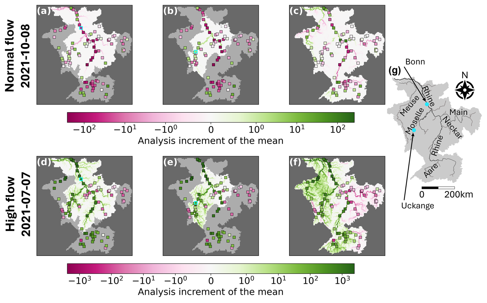
Figure 2 Analysis increments of the mean for a lead-time of 9 d for single station (a, b, d, e) and all station (c, f) experiments for the hindcasts generated on 8 October 2021 (upper panels) and 7 July 2021 (lower panels). Assimilated stations for the single station experiments (cyan outline) are the Bonn station on the Rhine (a, d) and the Uckange station on the Moselle (b, e). The shaded region of the catchment is outside the localisation length of the assimilated station. Markers show the innovation at all stations. Catchment area: 195 300 km². Panel g shows the Rhine-Meuse catchment and highlights the rivers and stations discussed within this section.

In Fig. 2, the shaded regions show the parts of the catchment that are outside the localisation region for the assimilated observation. The number of grid-boxes within the localisation regions of the Bonn and Uckange stations differ because the distance is calculated along the river network and the channel length within each grid box is not constant (4662 grid boxes and 2451 grid boxes, respectively). Increasing (decreasing) the localisation length scale results in a more (less) gradual dampening of the analysis increments and more (fewer) grid-boxes being impacted by a single observation (not shown). The square markers indicate the innovation – the difference between the observation and the error-corrected ensemble mean prior to the update step (Fig. 2). Ideally, the analysis increment (background colour in Fig. 2) should reflect similar spatial behavior to the innovations within the localisation region. This would imply the ensemble is being adjusted towards the observations at each station.

For the October experiment, the innovation at Bonn is negative and results in negative analysis increments across the domain (Fig. 2a). For the Uckange experiment, the innovation is positive and the analysis increments are also all positive (Fig. 2b) indicating positive ensemble covariances. For both experiments, the analysis increments match the sign of the innovations at neighbouring stations (Fig. 2a and b), but at greater distances this is not the case. For example, the innovations along the Rhine in the Uckange experiment are negative whilst the analysis increments are positive.

The localisation implemented in this study allows the assimilated observations to influence the error ensemble both up- and downstream, although the influence is dampened at longer distances. We here discuss whether this choice of implementation is useful by studying the spatial patterns of the innovations. Focusing first on the Bonn experiment for October (Fig. 2a), we see that downstream (north) of the assimilated observations the innovations can be both positive and negative. Upstream of the assimilated observation the innovations are negative, matching the innovation at the Bonn station. The assimilation of the observation at Bonn is therefore primarily beneficial upstream, with some benefit also seen at specific locations downstream. For the Uckange experiment (Fig. 2b), the pattern is reversed with downstream innovations showing more consistency with the innovation at the assimilated location. The inconsistent spatial patterns could be because, in the LETKF, we update the errors rather than the river discharge directly. The errors are dependent not only on the observed hydrological conditions but also the model structure and configuration. The spatial structure of the errors may therefore extend both up- and downstream. For example, if the drainage area within an upstream grid-box is overestimated due to the hydrological model spatial resolution, all grid-boxes downstream will be impacted by that overestimation. The benefit, in terms of consistency between the innovations and analysis increments, that is seen both up and downstream suggests that the localisation implementation is appropriate. However, we note that there may be additional factors other than distance, that could be included in the localisation to better modulate the observation influence (e.g., river confluences, regulation, or river size).

In the July experiments, we see that the innovations both up and downstream of the assimilated observations are positive, matching the innovations at the Bonn and Uckange stations, respectively. For the July experiment, the innovations are spatially homogeneous for greater distances along the river network (Fig. 2d and e). This indicates a greater spatial correlation length, likely due to the low-pressure system which covered large parts of the west of the catchment during this period (Mohr et al., 2023). The different correlation scales suggest that an adaptive localisation length scale may be beneficial.

The spatial heterogeneity for the October experiments suggests that assimilating a single observation cannot correct the entire domain. However, when all observation are assimilated the analysis increments vary across the domain, demonstrating the method's ability to adapt to the errors on different stretches of the river. In both all-station experiments (Fig. 2c and f), the analysis increments vary smoothly along the river network, which suggests the error-corrected ensemble will also change gradually. This is important because it ensures the hindcasts remain spatially consistent, with no abrupt transitions between adjacent grid boxes.

In general, for the July experiment, small rivers exhibit larger increments than in the October experiment. This indicates the assimilated observations have a greater impact across more of the domain. For October, the assimilation of an observation at Bonn results in the largest analysis increments near the observation location, with the increments diminishing to zero at distances greater than 524 km due to localisation (Fig. 2a). Interestingly, in the Uckange experiment, the largest increments occur not near the station, but along the Rhine near the confluence with the Moselle (Fig. 2b). In both experiments, the increments tend to be larger along bigger rivers, with smaller rivers showing smaller increments. This occurs due to large ensemble covariances between the location of the assimilated observation and locations along the bigger rivers (Fig. 3).

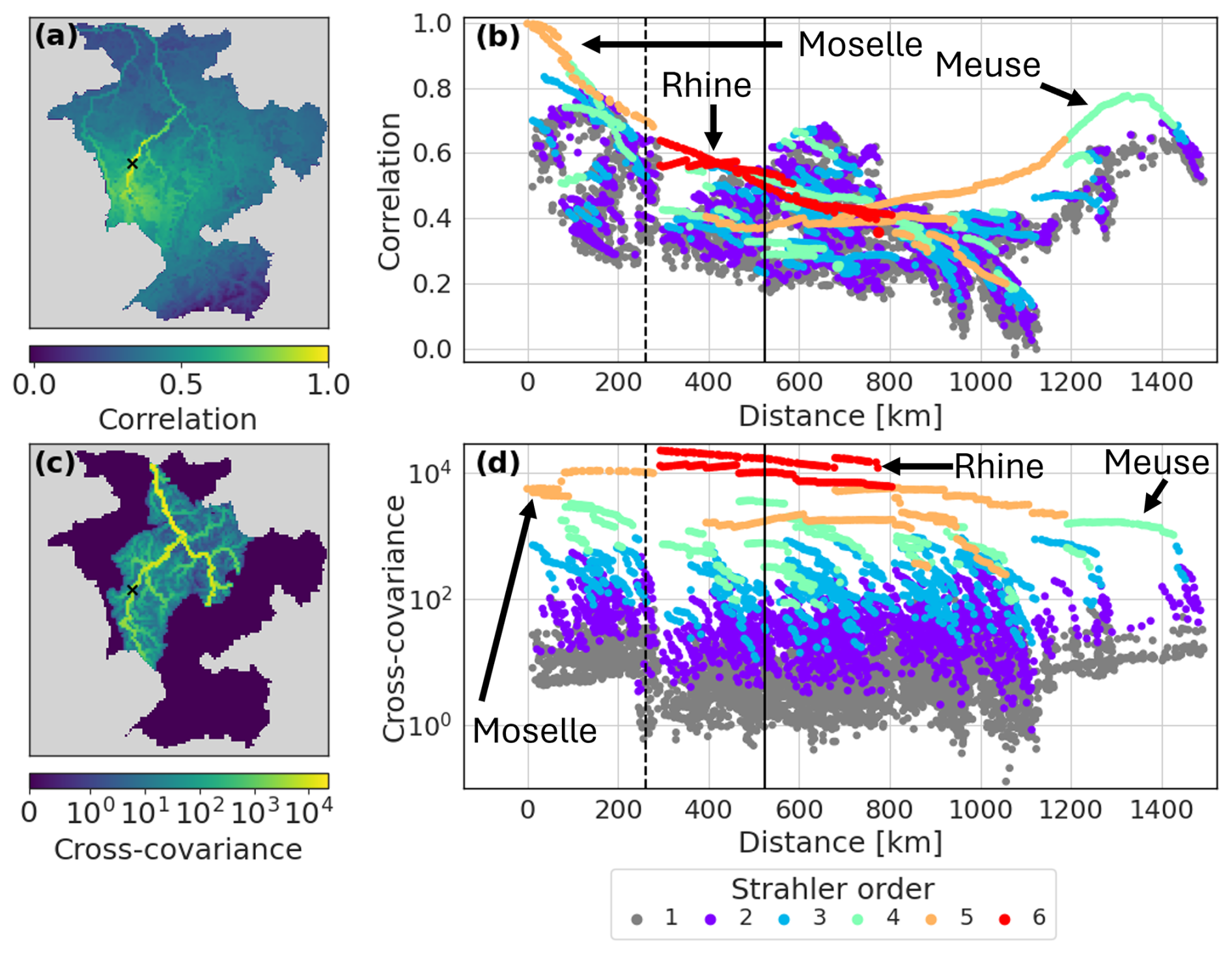
Figure 3 Ensemble correlations (upper panels) and cross-covariances (lower panels) between the error ensemble and the hindcast component of the augmented ensemble averaged across all all-station experiments. (a) Map of the correlation between the Uckange station and all other grid-boxes and (c) the same for the cross-covariances. (b) Scatter plot of the correlation between the Uckange station and all other grid-boxes and (d) the same for the cross-covariances. Grid-boxes on rivers discussed in the text are broadly indicated by the arrows. Dashed black line shows the localisation length scale and the solid black line shows the effective cut-off point beyond which the observation has no impact.

The spreading of observational information along the river network is dictated by the cross-covariances of the augmented ensemble prior to the update step. The magnitude of the cross-covariance between two locations depends on the correlation between the locations and the ensemble variance at both locations. The correlation between the location of the Uckange station and any grid-box is highest along the same river stretch (the Moselle) and decreases at longer distances from the station (Fig. 3a). Nearby grid boxes that are not on the same river stretch have lower correlations in general (Fig. 3a and b). Downstream from the Uckange station the correlation is highest along the Moselle and downstream along the Rhine. On the other hand, the correlation upstream is more uniform across the grid-boxes (Fig. 3b). Whilst there are regions in the south of the catchment for which the correlation is small, in general there is a correlation of around 0.3 even with distant locations (Fig. 3b). This is likely spurious correlation and exemplifies the need for localisation. The correlations begin to rise again at longer distances due to grid-boxes that are geographically close to the station but the distance along the river network is large, such as the Meuse (Fig. 3b). Note that the similarity between the localisation length scale (dashed line) and the distance between the Uckange station and grid-boxes on the Rhine (change from a Strahler order of 5 to 6) is coincidental but does suggest that the method for defining the localisation length scale is capable of capturing the order of magnitude of the relevant spatial scales for the Rhine catchment.

Despite lower correlations, the magnitude of the cross-covariances are larger along the Rhine than for grid-boxes closer to the Uckange station on the Moselle (Fig. 3c). Whilst the correlation is dependent on distance, the magnitude of the cross-covariances is primarily dependent on the size of the river (note the horizontal bands of Strahler orders (a measure of stream size where larger orders indicate larger rivers Strahler, 1957) in Fig. 3d). Larger cross-covariances can lead to larger analysis increments as can be seen in Fig. 2b where the analysis increments along the Rhine are larger than those along parts of the Moselle. Localisation enforces a dependence on distance such that observations have less impact on large rivers very far from the station but this may not outweigh the larger cross-covariances.

7.1.2 Lead-time dependence of the analysis increments

Here, we investigate how the impact of assimilating observations changes over different lead-times. Figure 4 shows the trajectories of the three intermediate ensembles used in the LETKF for the 7 July hindcast for a single-station experiment where observations are assimilated at the Uckange station: the raw hindcast (left columns), the hindcast component of the augmented ensemble (middle columns), and the error component of the augmented ensemble (right columns). It should be noted that none of these ensembles are the final error-corrected ensemble but intermediate ensembles used in the LETKF. The lower panels show the trajectories at the Bonn station for which no observations are assimilated during this experiment. By plotting the raw hindcast trajectories and the observations we can visualise the errors to be estimated. We can see that for both stations the error of the hindcast mean is negative (observations are smaller than the hindcast mean) for lead-times up to 8 d, and positive at longer lead-times. Whilst this behaviour is similar for the Bonn station, the magnitude of the error is different by a factor of 10 at most lead-times.

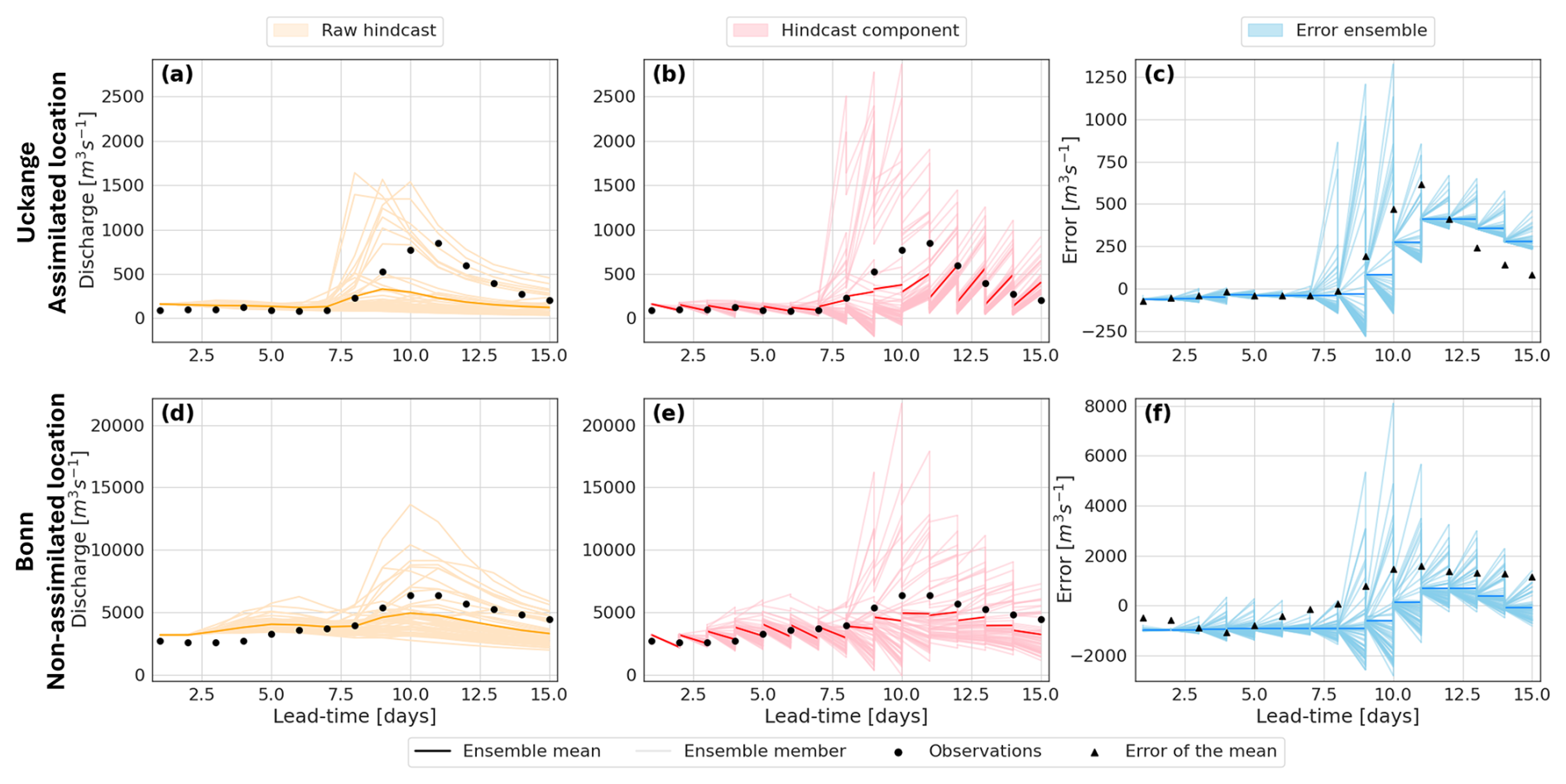
Figure 4 Ensemble trajectories for a single station experiment for the hindcast generated on 7 July 2021 for the location of the assimilated observation (Uckange station on the Moselle; panels a–c) and a location where an observations is not assimilated (Bonn station on the Rhine; panels d–f). The plots show the trajectory of all members and the ensemble mean of the raw hindcast ensemble (left panels), the hindcast component of the augmented ensemble (middle panels), and the error ensemble members (right panels; different y axis scale). Markers show the river discharge observations (a, b, d, e), and the error of the raw hindcast mean (c, f).

The middle column of Fig. 4 shows the hindcast component of the augmented ensemble. To propagate this component between time steps without rerunning a hydrological model, we assume that the raw hindcast is a reasonable approximation of the analysis state (discussed in Sect. 4.1). As expected, this assumption results in a sub-optimal ensemble mean estimate. For example, at lead times beyond 10 d at Uckange, the update moves the ensemble mean further from the observations (Fig. 4b), and a similar effect is seen at Bonn (Fig. 4e). Also by using the precomputed ensemble, the assimilated observations do not update the ensemble perturbations; although the perturbations do change between lead-times as the precomputed ensemble is lead-time dependent. This assumption ensures the analysis hindcast component is always physically plausible (e.g., the river discharge is always positive as this is a constraint within LISFLOOD), and provides a reasonable estimate of the uncertainty as the raw hindcast is generated using the output from an ensemble NWP. Additionally, at each timestep we aim to correct the raw hindcast, therefore this assumption provides consistency between the hindcast component and the error component of the augmented ensemble.

It is the error ensemble that is most important for our application (Fig. 4c and f). Despite the non-optimal formation of the analysis augmented ensemble, the error ensembles are updated beneficially, with the analysis error ensemble mean moving closer to the error of the raw hindcast mean (i.e., the difference between observations and the hindcast mean) at each lead-time for the assimilated location (Fig. 4c) and the non-assimilated location (Fig. 4f). At short lead-times, the updates to the error ensemble at the Bonn station do not appear to be beneficial (Fig. 4f). However, as this experiment only assimilates observations from one station this discussion should be considered a demonstration of how the method updates ungauged locations rather than an evaluation of the error-corrected ensemble (which is provided in Sect. 7.2). First we note that the updates at the assimilated location do not result in the error ensemble mean (dark blue line) matching the error of the mean (markers). This is expected and is due to the consideration of the observational uncertainty within the LETKF. This ensures spatial consistency across assimilated and non-assimilated locations, whilst combining the modelled and observed data to estimate the true state of the system across the domain.

The error ensemble is narrow after the update step and it is the covariance inflation that increases the spread between time steps. The spread of the hindcast is due to meteorological forcings, predominantly precipitation. Therefore, in general, the hindcast spread is larger for longer lead-times as the precipitation forecasts become more uncertain. Since the covariance inflation technique presented here results in the blending of the hindcast perturbation matrix with the error ensemble from the previous timestep, this behaviour in the hindcast spread is transferred to the error ensemble. As demonstrated in Fig. 4c and f, this can result in the error ensemble spread being large for the rising limb of an event and smaller for the falling limb. This can result in the error not being updated sufficiently and the spread of the analysis state being too narrow, as seen after the peak in Fig. 4c and discussed later along with Fig. 5b.

7.2 How skillful are the error-corrected ensemble hindcasts?

In this section, we investigate whether the updated ensemble is more skillful than the raw hindcast ensemble. Using leave-one-out experiments we evaluate the ensemble mean and ensemble spread at proxy-ungauged locations. The hydrographs in Fig. 5 show the raw and error-corrected ensembles for three proxy-ungauged locations from the leave-one-out experiments. The hydrographs are used to illustrate the method's ability to correct the ensemble and some of the limitations.

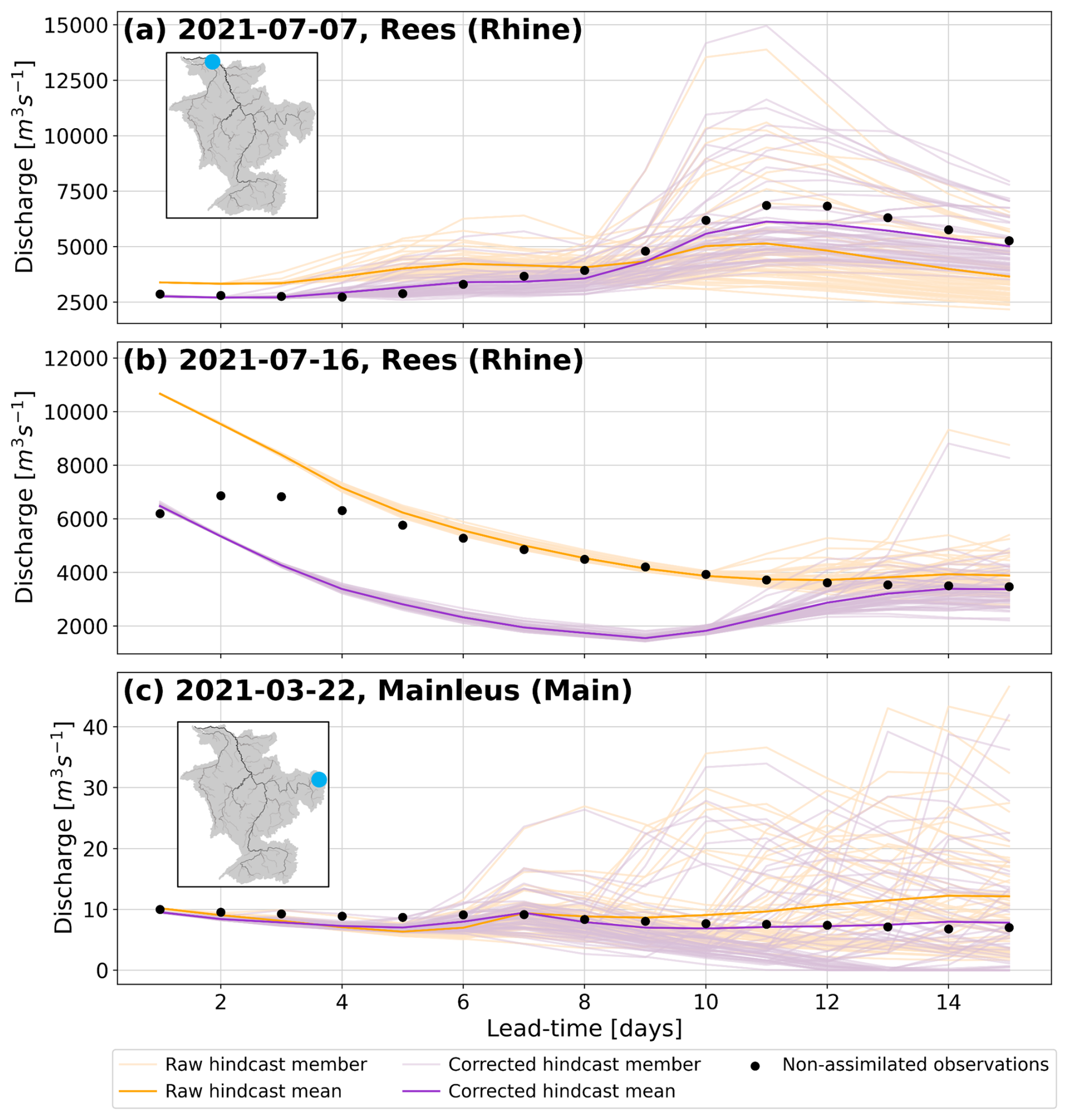
Figure 5 Raw and error-corrected hydrographs for proxy-ungauged locations in leave-one-out experiments at the Rees station on the Rhine (upstream area: 159 320 km³) and the Mainleus station on the Main (upstream area: 1164 km³). Catchment illustrations indicate the location of the station (see Fig. 2 for river names and scale).

7.2.1 Skill of the ensemble mean

To investigate the skill of the ensemble mean we calculate the correlation, mean bias, variability bias and the N-RMSE for each station and each lead-time. Figure 6 compares the skill of the ensemble means of the raw and the error-corrected ensembles focusing on the spatial dependency of the skill (a–d), and the lead-time dependency of the skill (e–h).

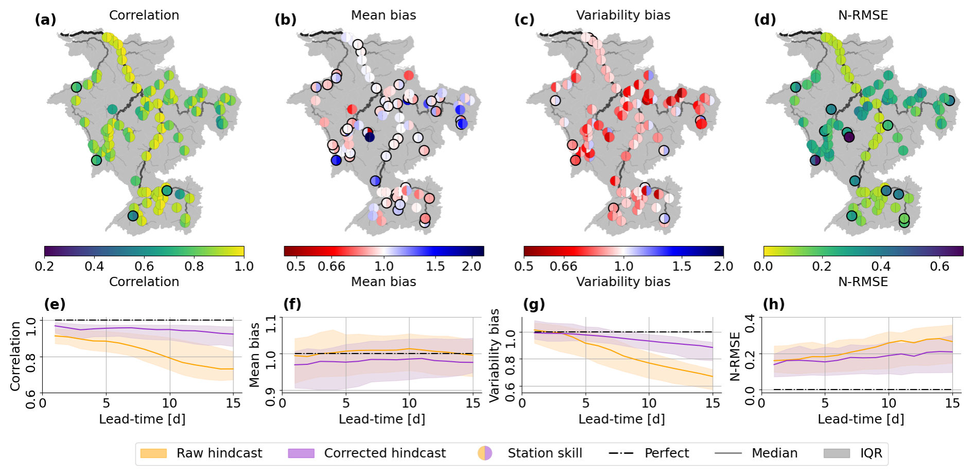
Figure 6 Skill of the ensemble means in terms of the correlation (a, e), mean bias (b, f), variability bias (c, g) and normalised root mean square error (N-RMSE; d, h). The catchment maps show the metric averaged across all lead-times at all 89 stations (a–d). The left (right) half of the markers show the skill for the raw (error-corrected) ensemble. Black outlines indicate stations for which the updated ensemble has worse skill than the raw hindcast ensemble (Correlation: $\mathrm{4}/\mathrm{89}$, Mean bias: $\mathrm{42}/\mathrm{89}$, Variability bias: $\mathrm{10}/\mathrm{89}$, N-RMSE: $\mathrm{14}/\mathrm{89}$). Line plots show the distribution of the metric pooled over all 89 stations for each lead-time for the raw (orange) and error-corrected (purple) ensembles (e–h). The solid line shows the median value of the metric and the shaded region shows the interquartile range (IQR) of the metric. A perfect score for the metric is shown by the dashed black line.

The error-corrected ensemble means show a stronger correlation with observations than the raw hindcast ensemble means, with an average increase from 0.82 to 0.92 (not shown). Figure 5a shows an example of how the error-corrected ensemble can better capture the dynamics of the river discharge resulting in an increased correlation. It can be seen that the resulting ensemble is temporally consistent (i.e., does not have improbable changes between time steps). The correlation is worsened compared to the raw hindcast ensemble at four stations (Fig. 6a). Focusing on the two most southern of these stations, we see that the correlation values of the raw ensembles at nearby stations are very different compared to the correlation at the two stations of interest (note the much lighter colours for nearby stations; Fig. 6a). The ensemble covariances are not capturing this change in regime correctly so the observational information is not being advantageously spread between these rivers. The remaining two stations that have degraded correlation are the most upstream stations on their rivers. At these stations the updates made to the error-corrected ensemble are dependent on observations assimilated downstream. The assimilated observations are therefore providing information about a past state of the river upstream which could be the cause of the decreased correlation (a measure of timing errors) at these upstream stations. Whilst most upstream stations are improved by the error-correction method, stations which have much smaller upstream areas than their closest downstream station tend to be improved less than those that have a similar upstream area, particularly if the distance to the neighboring station is large.

Just over half of the stations (47) show improvement in the mean bias averaged across all lead times (Fig. 6b), but no clear spatial pattern emerges, as most rivers have a mix of improved and worsened stations. This spatial heterogeneity is also seen in the raw hindcast ensemble, with stations on the same river stretch often showing different biases. For example, stations on the Neckar and upstream of the Meuse show stations that are under- and overestimated, as well as stations with very little bias. The heterogeneity suggests local factors, which are not fully captured in the hydrological model, considerably influence flow bias. Stations showing the most improvement tend to have similar mean bias values to their neighboring stations in the raw hindcast ensemble, such as on the middle stretch of the Meuse, where four stations with similar biases show improvement (Fig. 6b). Spatial patterns of errors that are related to domain-wide model structure rather than local factors, such as weirs, are more likely to be portrayed by the ensemble covariances allowing observational information to be more helpfully spread along the river network.

The raw hindcast ensemble mean generally underestimates flow variability, with a variability bias below 1 (red in Fig. 6c). The error-corrected ensemble improves this, although there is an increase in the frequency of overestimation of the flow variability. Stations where the error-corrected ensemble overestimates the variability are often the most upstream station on their rivers (e.g., Plochingen station on the Neckar) or are closer to downstream neighbours (e.g., Chooz station on the Meuse). This suggests the hindcast covariances between downstream stations and upstream locations are too large, causing excessive adjustment at upstream locations. Ten stations show worsened variability bias, including two stations downstream on the Rhine (Fig. 6h). For the two stations on the Rhine, the degradation is caused by the forecasts of the falling limb of a flood peak in July (Fig. 5b). Here, the hindcast uncertainty was very small at short lead-times, causing the analysis to ignore observations, leaving the error ensemble relatively unchanged, despite changes in the error behaviour after the peak (also shown in Fig. 4f).

Overall, the error-corrected ensemble reduces the N-RMSE but there are 14 stations where the skill is reduced. Typically, these stations are on the upstream reaches of their respective rivers (Fig. 6d; see discussion on correlation). Interestingly, the N-RMSE does not follow the same spatial pattern as the mean bias. This divergence indicates that the correction method is more effective at reducing large errors than at addressing systematic biases. One possible explanation is that the error vectors adjust too slowly to changes in forecast errors between time steps. This slow adjustment is particularly problematic when errors fluctuate around 0 m³ s⁻¹, since alternating positive and negative deviations may not be corrected quickly enough and can accumulate into a worsening mean bias. When the error magnitude is large, the gradual adjustment is less detrimental because the sign of the error is usually captured correctly even if its magnitude is not. However, at upstream stations, where rivers are smaller and respond more quickly to rainfall, large errors often persist for shorter durations, making the slow adjustment of the error vectors more detrimental. This likely contributes to the increase in N-RMSE observed at these upstream stations. Further development of the method – for example, allowing the error vectors to evolve during the propagation step of the LETKF in addition to the update step – could enable faster adaptation to changing forecast errors.

The raw and error-corrected ensemble means both decrease in skill in terms of correlation, variability bias, and N-RMSE with increasing lead-times. The raw hindcast ensemble loses skill more quickly in particular for lead-times longer than 5 d (Fig. 6e–h). The uncertainty in the observations is not lead-time dependent. However, Fig. 3d shows that the ensemble covariances do change across lead-times, increasing for longer lead-times. The greater gain in skill for longer lead-times is likely due to larger covariances allowing the observations to have more influence (e.g., in Fig. 5b). However, the decrease in skill of the error-corrected ensemble means at longer lead-times suggests that the ensemble covariances are not as accurate at longer lead-times.

7.2.2 Skill of the ensemble distribution

The reliability of the ensemble distribution is assessed using rank histograms at different lead times (Fig. 7). At short lead times, the raw hindcast ensemble is underdispersed, due to the use of a single set of initial conditions (Fig. 7a). Although the error-corrected ensemble shows slight improvement, it remains overconfident with minimal correction to the spread. Both the raw and error-corrected ensembles generally appear unbiased, with observations falling both above and below the ensemble predictions at similar frequencies. However, some bias may be masked by the narrow ensemble spread as it is known that some stations are biased (Fig. 6b), likely contributing to the peaks at ranks 0 and 51 in the rank histograms.

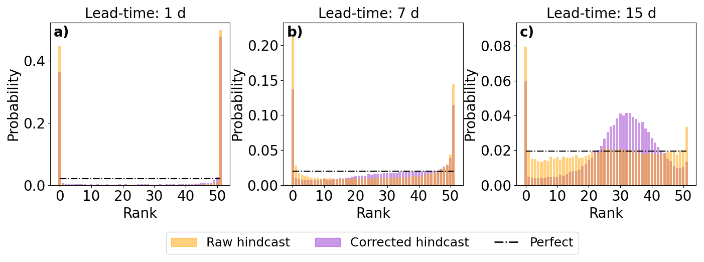
Figure 7 Reliability of the ensemble. Histograms show the rank of the ensemble pooled over all forecasts and stations for lead-times of 1 d (a), 7 d (b), and 15 d (c).

As the lead-time increases, the spread of both ensembles becomes more reliable, and fewer observations fall outside the ensemble (Fig. 7b). However, even at a 15 d lead time, both ensembles show a tendency to overestimate observations, leading to a peak at rank 0, mostly due to a few stations consistently overestimating flow (Fig. 6b). Up to 7 d lead times, the rank histograms for both raw and error-corrected ensembles show similar shapes. Beyond 7 d, the raw hindcast ensemble's histogram flattens, suggesting a reliable ensemble, while the error-corrected ensemble shows a peak around ranks 25–35, suggesting overdispersion (Fig. 7c). The left-skewness of the histograms is likely due to the inherent skewness in river discharge distributions. The LETKF update step seeks to minimise the difference between the ensemble mean and the true state of the system. The ensemble mean is often larger than the ensemble median leading to the observations falling in ranks above 25 if the adjustment method is successful at minimising the error of the mean (Fig. 5a and c).

As discussed in Sect. 4.1, the Kalman filter is not restricted to ensure positive discharge and there is therefore a need to adjust the error ensemble before correction of the hindcast. Enforcing non-negative discharge was necessary, for example, for the Mainleus station on the Main for the hindcast generated on the 22 March 2021 (Fig. 5c). Whilst the ensemble mean is error-corrected at most lead-times, several members indicate river discharge values of 0 m³ s⁻¹. The river discharge is below 10 m³ s⁻¹ but a zero flow is unlikely in reality. This suggests the ensemble spread is not sufficiently corrected even though the ensemble mean is improved as is also suggested by Fig. 7c.

8 Discussion

In general, the proposed data-assimilation-inspired method successfully spreads observational information along the river network, thereby improving the skill of the ensemble mean at proxy-ungauged locations (i.e, locations where observations were withheld for cross-validation). Locations downstream from assimilated observations are improved most although locations upstream are usually improved as well, even if they are far from neighbouring stations. This is likely due to two reasons: (1) constant biases in the river discharge estimates that are propagated downstream and hence can be accounted for when a downstream observation is assimilated, and (2) the daily aggregation of the river discharge extending the time period for which a downstream observation provides relevant information. If the error patterns of the ensemble mean at a location differ from those at nearby stations the method struggles to spread the observational information correctly. At shorter lead-times the reliability of the ensemble is slightly improved due to the decrease in the error of the ensemble mean. However, at longer lead-times the ensemble spread is often too large leading to an under-confident forecast.

The ability of the method to correct the forecasts typically depends on the consistency of the error vectors between nearby locations. The localisation method implemented here depends only on the distance from the station along the river network. The method does successfully correct the forecast both up- and downstream; however, if the station is on a different river, or if there is a confluence between the station and the grid-box of interest, the errors are often not consistent for as long a distance along the river network. Therefore, it could be beneficial to investigate the impact of including information about the river stretch into the localisation length scale. Additionally, the errors were found to be more consistent when the catchment was impacted by large-scale weather systems. It may therefore be useful to incorporate information about the meteorological situation into the localisation function as well.

The covariance inflation method used here maintains consistency between the spread of the error ensemble and the spread of the hindcast (Sect. 5.2). This successfully stops the error ensemble from collapsing such that the observations are not ignored. However, in situations where the uncertainty of the hindcast ensemble is over- or under-estimated the covariance inflation does not correct the error ensemble covariances correctly. This can lead to the observations being ignored as for short lead-times in Fig. 5b. Additionally, if the hindcast perturbations do not provide an accurate estimate of the true error ensemble perturbations, this method may introduce errors which could be the cause for the slight degradation in skill of the ensemble mean with lead-time shown in Fig. 6e, g, and h. Correcting the spread of the hindcast before using it in the inflation of the error covariances could solve this issue. Covariance inflation techniques that use the innovation statistics could be used to first adjust the hindcast ensemble (e.g., Kotsuki et al., 2017). Alternatively, a lower threshold for the variance of the ensemble could be set – say 10 % of the ensemble mean, similar to the observation error covariance matrix, or the root mean square-error of the initial conditions. However, caution is needed not to artificially inflate the covariances too much such that the analysis increments become too large.

As discussed in Sect. 7.2.2, the resulting ensemble must be adjusted in some cases to avoid negative discharge values (Sect. 4.1). This does in some cases lead to ensemble members close to 0 m³ s⁻¹ when a zero flow value is unlikely (e.g., Fig. 5c). This occurs due to the analysis increment being larger in magnitude than the value of some of the raw ensemble members. In general, this is due to the skewed distribution of discharge (Bogner et al., 2012). Future work could look into applying anamorphosis, or normalising transformations, to make the ensemble distribution more Gaussian-like (Nguyen et al., 2023; Bogner et al., 2012). This was not done in this proof-of-concept study for simplicity and to facilitate the interpretation of the errors. The results also showed that the covariances between grid boxes on larger rivers and the station locations tend to be large even when the correlation is small. This is due to larger rivers having larger variances which is partially due to their larger river discharge magnitudes. Localisation enforces a distance dependence on the covariance magnitudes. However, transforming the river discharge values to be comparable across the domain may help regulate the covariances based on river size. A transformation between river discharge and specific discharge (river discharge divided by upstream area) could be used to ensure that the ensemble covariances more accurately represent the true relationship between locations.

In this study, the initial estimate of the error ensemble mean is defined using the observations and the simulation forced with meteorological observations from the 10 d before the forecast. The average difference between the observations and simulations is calculated at gauged locations and interpolated to every grid-box using inverse distance weighted interpolation. The aim is to provide a physically plausible first guess of the errors which is then updated at each timestep. By taking the average over a 10 d period, we aim to capture the biases of the hydrological model but also to allow for seasonal/dynamic variation in this bias. However, the choice of 10 d has not been tuned, and may be more applicable to larger catchments with slowly changing errors than for smaller catchments (Matthews et al., 2022). Further research into the accuracy of the initial error ensemble, and how it influences the skill of the error-corrected ensemble, is needed. It should be noted that this component of the method is an implementation choice and can be adjusted depending on system configuration and data availability. The only requirement is that the initial error ensemble is physically plausible as there is no warm-up period within this application (Kim et al., 2018).

We assume that the errors are sufficiently slowly changing such that a persistence model can be used to propagate the errors between timesteps. It should be noted that the LETKF updates the errors at each timestep so the analysis errors used to correct the hindcasts are not constant for all timesteps. However, the assumption that the errors are slowly changing is likely only true for larger rivers that respond more slowly. Future studies could investigate the use of a simple time-varying evolution model. The model would need to be simple enough that the calculations do not add too much computational time to the method. Additionally, the error values at every grid-box would need to be evolved; therefore, the evolution model should either rely only on the model output or must be spatially interpretable if using observations. For example, a model dependent on the hindcast river discharge magnitude could be used to evolve the errors between timesteps.

The leave-one-out approach used in this study allows the corrected ensembles to be assessed at proxy-ungauged locations. However, only one station is omitted at a time. Future work could use a block cross-validation strategy whereby multiple stations are omitted simultaneously (Roberts et al., 2017). This would allow the impact of the density of stations and their specific locations along the river network to be investigated more thoroughly (Rakovec et al., 2012). The impact of not having any observations along a river stretch could also be more thoroughly investigated. One benefit of this method is that the assimilated observations do not necessarily need to be traditional in-situ observations but could come from Earth Observation (EO;  Durand et al., 2023), crowdsourced or community observations (Le Coz et al., 2016; Etter et al., 2020), or camera-based sensors (Vandaele et al., 2021). The key requirement is that an observation operator can be defined. Observation operators map the state of the system from state space to observations space. In our study the observation operator selects the grid box that represents the location of the station on the modelled river network. The mapping of the station locations from the physical river network to the modelled river network is not trivial and several studies have attempted to automate this step (Isikdogan et al., 2017; Li et al., 2018). If this mapping is incorrect then representation errors can be introduced (Janjić et al., 2018). For example, if a station on a bypass channel is incorrectly located on the main channel, observations from the station will undoubtedly provide erroneous information in the update step.

The code developed for this study is designed to allow for research flexibility rather than operational efficiency. However, the error-adjustment of a single forecast took on average 8.5 min for the whole of the Rhine-Meuse catchment – a large catchment. This suggests that, with proper parallelisation, the method could be operationalized and applied to all gauged catchments in Europe. Before that, though, the method needs to be evaluated on additional catchments. The Rhine was selected because it is highly gauged, but this also means that the raw ensemble's skill is relatively high due to the effectiveness of the hydrological model calibration process. This could influence the method's performance in two ways: (1) the error ensemble may evolve more linearly than in less calibrated catchments, and (2) the hindcast ensemble’s covariance may better represent the covariances between the estimated errors. The next step should be applying this method to a catchment with lower skill than the Rhine.

The method presented in this study spreads observation information along the river network but cannot yet be used as a post-processing method because observations from the hindcast period (the future) are assimilated. We envisage the method being developed further to make it applicable operationally as a hydrological forecast post-processing method. Nevertheless, it may still be useful in certain situations, such as post-event analysis. After a flood event an assessment is often performed estimating the severity of the event as well as potential causes and mitigating factors. However, in-situ river gauges only present a snapshot of the event at specific locations and are often damaged during flood events, resulting in missing or incorrect data. EO estimations of river discharge could fill in some of the gaps but this would depend on the satellite's orbit and its availability at the right time (Douben, 2006). Reanalysis is another option, but it requires additional hydrological model runs and may contain errors due to the structure of the hydrological model or errors in the meteorological observations. The method proposed here could offer a domain-wide estimate of observations without requiring additional model runs or a “warm-up” period typically needed in hydrological simulations to stabilize antecedent water storage within the catchment.

9 Conclusion

We present and evaluate a data-assimilation-inspired method for spreading observation information from gauged to ungauged locations in a post-processing environment. This method enables the error correction of ensemble simulations at all grid boxes. The method utilises state augmentation within an LETKF framework to estimate an ensemble of error vectors. The error vectors are then used to correct each hindcast ensemble member separately.

Overall, the method successfully reduces the errors of the ensemble mean at ungauged locations in leave-one-out experiments. The adjusted ensemble mean has a higher correlation with the observed river discharge and is more able to capture the variability of the river discharge at a point. Whilst the magnitude of the errors is reduced the ensemble spread is not adjusted sufficiently resulting in an under-confident ensemble spread at longer lead-times. The adjusted ensembles are spatially and temporally consistent with the river discharge predictions showing smooth evolution both between grid-boxes on the same river and between lead-times. The method is most limited at locations further upstream than the assimilated observations and for hindcasts with unrealistically small ensemble variance, which most often occurs at shorter lead times. These limitations could be reduced by further investigation into the localisation approach, for example having a different localisation length upstream and downstream from the assimilated observation, and the covariance inflation approach, which may involve applying a spread-correction to the hindcast ensemble as well as the error ensemble.

Our method of spreading observation information could be used to improve post-event analysis. However, as the computational requirements and processing time are both small the method could also be developed further to allow for its application to the post-processing of operational forecasts. The prediction of river discharge at ungauged locations is a crucial challenge for hydrological research and once successfully achieved will allow for better preparedness for floods.

Appendix A: Kalman gain matrix decomposition

The Kalman gain matrix has the following form for timestep k:

$$\begin{array}{}\text{(A1)}& {\mathbf{K}}_k={\mathbf{P}}_k^{\mathrm{f}}{\mathbf{H}}_k^{\top }{\left({\mathbf{H}}_k{\mathbf{P}}_k^{\mathrm{f}}{\mathbf{H}}_k^{\top }+{\mathbf{R}}_k\right)}^{-\mathrm{1}}\end{array}$$

where ${\mathbf{P}}_k^{\mathrm{f}}$ is the prior ensemble covariance matrix, R_k is the error-covariance matrix of the observations, and H_k is the observation operator (Livings, 2005; Hunt et al., 2007; Kalman, 1960). Substituting the definitions of the perturbation matrix and the observation operator for the augmented state given in Eqs. (9) and (11) gives:

$${\mathbf{K}}_k={\mathbf{W}}_k^{\mathrm{f}}{\mathbf{W}}_k^{fT}{\mathbf{H}}_k^{\top }{\left({\mathbf{H}}_k{\mathbf{W}}_k^{\mathrm{f}}{\mathbf{W}}_k^{fT}{\mathbf{H}}_k^{\top }+{\mathbf{R}}_k\right)}^{-\mathrm{1}}.$$

This can then be decomposed into the hindcast and error components as

$$\begin{array}{}\text{(A2)}& \begin{array}{rl}{\mathbf{K}}_k& =\left(\begin{array}{c}{\mathbf{K}}_{{\mathit{x}}_k}\\ {\mathbf{K}}_{{\mathit{b}}_k}\end{array}\right)=\left(\begin{array}{c}{\mathbf{X}}_k^{\mathrm{f}}+{\mathbf{B}}_k^{\mathrm{f}}\\ {\mathbf{B}}_k^{\mathrm{f}}\end{array}\right)({\mathbf{H}}_k{\mathbf{X}}_k^{\mathrm{f}}+{\mathbf{H}}_k{\mathbf{B}}_k^{\mathrm{f}}{)}^{\mathrm{T}}\\ & \cdot \left(\right({\mathbf{H}}_k{\mathbf{X}}_k^{\mathrm{f}}+{\mathbf{H}}_k{\mathbf{B}}_k^{\mathrm{f}}\left)\right({\mathbf{H}}_k{\mathbf{X}}_k^{\mathrm{f}}+{\mathbf{H}}_k{\mathbf{B}}_k^{\mathrm{f}}{)}^{\mathrm{T}}+{\mathbf{R}}_k{)}^{-\mathrm{1}}\end{array}\end{array}$$

The analysis of the ensemble mean of the augmented states is therefore given by

$$\begin{array}{}\text{(A3)}& {\stackrel{\mathrm{‾}}{\mathit{w}}}_k^{\mathrm{a}}=\left(\begin{array}{c}{\stackrel{\mathrm{‾}}{\mathit{x}}}_k^{\mathrm{f}}+{\stackrel{\mathrm{‾}}{\mathit{b}}}_k^{\mathrm{f}}\\ {\stackrel{\mathrm{‾}}{\mathit{b}}}_k^{\mathrm{f}}\end{array}\right)+\left(\begin{array}{c}{\mathbf{K}}_{{\mathit{x}}_k}\\ {\mathbf{K}}_{{\mathit{b}}_k}\end{array}\right)({\mathit{y}}_k-{\stackrel{\mathrm{‾}}{\mathit{y}}}_k^{\mathit{x}}),\end{array}$$

where ${\stackrel{\mathrm{‾}}{\mathit{x}}}_k^{\mathrm{f}}$ and ${\stackrel{\mathrm{‾}}{\mathit{b}}}_k^{\mathrm{f}}$ are the ensembles mean of the raw hindcast and the prior error ensemble at timestep k, y_k is the observation vector, and ${\stackrel{\mathrm{‾}}{\mathit{y}}}_k^{\mathit{x}}$ is the model-observation ensemble mean.

Appendix B: Gaspari-Cohn function

The Gaspari-Cohn function is correlation function commonly used in data assimilation to define the localisation weights (Gaspari and Cohn, 1999). It has the following form:

$$\begin{array}{}\text{(B1)}& \mathit{\rho }\left(r\right)=\left\{\begin{array}{ll}\mathrm{1}-\frac{\mathrm{5}}{\mathrm{3}}{r}^{\mathrm{2}}+\frac{\mathrm{5}}{\mathrm{8}}{r}^{\mathrm{3}}+\frac{\mathrm{1}}{\mathrm{2}}{r}^{\mathrm{4}}-\frac{\mathrm{1}}{\mathrm{4}}{r}^{\mathrm{5}},& \mathrm{0}\le r\le \mathrm{1}\\ -\frac{\mathrm{2}}{\mathrm{3}}{r}^{-\mathrm{1}}+\mathrm{4}-\mathrm{5}r+\frac{\mathrm{5}}{\mathrm{3}}{r}^{\mathrm{2}}+\frac{\mathrm{5}}{\mathrm{8}}{r}^{\mathrm{3}}-\frac{\mathrm{1}}{\mathrm{2}}{r}^{\mathrm{4}}+\frac{\mathrm{1}}{\mathrm{12}}{r}^{\mathrm{5}},& \mathrm{1}<r\le \mathrm{2}\\ \mathrm{0},& r>\mathrm{2}\end{array}\right.\end{array}$$

where $r=d/c$ where d is the physical distance between two points, and c is the localisation length scale. The function has a value of 1 when r=0 and a value of 0 when r>2.