Equilibrium-approximated solutions to the reactive Lauwerier problem: thermal fronts as controls on reactive fronts in Earth systems

Rates of subsurface rock alteration by reactive flows are often independent of kinetic rates and governed solely by solute transport. This enables a major simplification that makes models tractable even for complex kinetic systems through the widely applied local equilibrium assumption. Here, this assumption is applied to the reactive Lauwerier problem (RLP), which describes non-isothermal fluid injection into a confined aquifer, leading to chemical disequilibrium. Specifically, the thermal changes drive temperature-dependent solubility variations, leading to undersaturation and dissolution or supersaturation precipitation reactions. Using this framework, solutions for reaction rate and porosity evolution are developed and analyzed, yielding a time-dependent criterion for their validity that incorporates time and thermal parameters. A key feature – the coalescence of thermal and reactive fronts – is used to explore their evolution over time in different settings. The applicability of the equilibrium model for important fluid–rock interaction processes is then examined and discussed, including sedimentary reservoir evolution and mineral carbonation in ultramafic rocks. Notably, the approach used here to extend thermal solutions for reactive processes suggests broader applicability. The findings also highlight that thermally driven reactive fronts, particularly near equilibrium, often become stationary after a relatively short period. As a result, their spatial evolution is governed by geological processes operating over much longer timescales.

1 Introduction

Natural and anthropogenic systems are often complex, involving intricate interactions between various processes, which makes developing a mechanistic understanding of the system challenging. However, the disparity in timescales between these processes often allows for significant simplification, as one process typically serves as the rate-limiting step that controls the system's overall evolution. This simplification, in turn, enables the recovery of the system's mechanistic behavior. Such systems range from climate science, where atmospheric and oceanic processes interact and operate at different timescales (Vallis, 2017), to multi-step biochemical processes and enzyme kinetics (Cornish-Bowden, 2013), traffic flow analysis (Lighthill and Whitham, 1955), epidemiology and disease spread (Anderson, 1991), economics (Solow, 1956), and crystal growth (Mullins and Sekerka, 1963).

Similarly, in geothermal systems, thermo–hydro–chemical (THC) processes often involve complex interactions. In particular, geochemical kinetics can be highly intricate, involving multiple species and reactions of varying orders, which are influenced by flow and transport dynamics and thermal variations (Appelo and Postma, 2004; Kolditz et al., 2016; Phillips, 2009). This complexity hinders the understanding of system behaviors and their description using tractable models. However, in many cases, the rate of transport is much slower than the reaction kinetics, effectively controlling the overall reaction rate. These conditions, known as transport-controlled, occur when the transport of reactants or reaction products dictates the reaction rate (Deng et al., 2016; Roded et al., 2020; Steefel and Maher, 2009).

Under transport-controlled conditions, the characteristic timescale of transport, t_A, is much larger than that of the reaction, t_R, with t_A≫t_R, and the system is close to chemical equilibrium (i.e., quasi-equilibrium). In such cases, the local equilibrium assumption is often invoked, and the assumption that the reaction rate depends solely on transport allows one to greatly simplify models (Andre and Rajaram, 2005; Lichtner et al., 1996; Molins and Knabner, 2019). The validity of the equilibrium assumption is determined by a large timescale ratio and the Damköhler number, Da, which, assuming a first-order surface reaction, is given by

$$\begin{array}{}\text{(1)}& \mathit{Da}={\displaystyle \frac{t_{\mathrm{A}}}{t_{\mathrm{R}}}}={\displaystyle \frac{l{A}_{\mathrm{s}}\mathit{\lambda }}{u_{\mathrm{A}}}}\gg \mathrm{1},\end{array}$$

where l is a local characteristic length scale, u_A denotes the characteristic Darcy flux [L T⁻¹], A_s is the specific reactive area (L² to L⁻³ of a porous medium), and λ is the kinetic reaction rate coefficient [L T⁻¹] (Lichtner et al., 1996; MacQuarrie and Mayer, 2005).

In this study, equilibrium-approximated solutions for geothermal systems are derived. These build upon and extend previous work (Roded et al., 2024b), in which thermally driven reactive transport solutions were developed within the framework of the Lauwerier solution (Lauwerier, 1955). The Lauwerier solution provides an analytical prediction of the thermal field development resulting from the injection of hot (or cold) fluid into a thin, non-reactive, confined layer system (Lauwerier, 1955; Stauffer et al., 2014).

The thermally driven reactive transport solutions developed by Roded et al. (2024b) integrate temperature-dependent solubility into a reactive flow formulation while incorporating the thermal field based on the Lauwerier solution. Specifically, this setting, referred to as the reactive Lauwerier problem (RLP), accounts for thermal variations that drive the system out of geochemical equilibrium, thereby triggering chemical reactions. These disturbances stem from shifts in mineral solubility within groundwater, where thermal fluctuations can induce conditions of either supersaturation or undersaturation. Over time, these thermally driven reactions lead to changes in rock porosity due to the precipitation, dissolution, or replacement of solid minerals and the associated volumetric changes (Phillips, 2009; Woods, 2015).

Depending on the natural solubility of the minerals in the system, an increase in temperature can lead to either dissolution or precipitation. This occurs because mineral solubilities can either decrease with temperature (retrograde solubility) or increase with it (prograde solubility; Jamtveit and Yardley, 1996; Phillips, 2009). A notable example includes the prograde solubility of silica, which commonly precipitates in geothermal systems from the cooling of fluids (Pandey et al., 2018; Rawal and Ghassemi, 2014; Taron and Elsworth, 2009). In contrast, carbonate minerals such as calcite and dolomite exhibit an inverse relationship with temperature and retrograde solubility, which is often pronounced and influenced by CO₂ concentration. Depending on the conditions, either rapid dissolution or rapid precipitation can occur in the case of common carbonate minerals (Andre and Rajaram, 2005; Coudrain-Ribstein et al., 1998).

Fluid recharge or injection under constrained physical and chemical conditions, as in RLP settings, is common in both natural and engineered geothermal systems and aquifers (Phillips, 2009; Stauffer et al., 2014). These include aquifer thermal storage, reinjection of geothermal water, and groundwater storage and recovery applications (Diaz et al., 2016; Fleuchaus et al., 2018; Maliva, 2019), as well as implications for mineral carbonation in mafic or ultramafic rocks (Kelemen et al., 2019; Roded and Dalton, 2024).

In what follows, the settings and equations are first described, which then serve to derive the equilibrium-approximated solutions for the RLP for both radial and planar flows. These solutions are then compared to the reference solutions from Roded et al. (2024b) to validate them and discuss their limitations, along with the derivation of specific criteria for the RLP setup. Next, a key feature of the coalescence of the thermal and reactive fronts under quasi-equilibrium conditions is used to examine their evolution. Interestingly, under certain conditions, thermally driven reactive fronts essentially cease to expand and become stationary after a short timescale, remaining governed by longer-term tectonic processes. The applicability of the equilibrium model to key processes, including sedimentary aquifer alteration and natural mineral carbonation, is discussed, along with an outlook for further theoretical developments.

2 Settings and the equilibrium model equations

This section describes the RLP under the equilibrium assumption and then outlines the specific settings and relevant governing equations. These equations define the THC equilibrium model (Phillips, 2009; Wood and Hewett, 1982) used to derive the solutions in this work. A comprehensive review of the more general RLP framework and its main assumptions is provided in Roded et al. (2024b) and further revised in Appendix A of this work.

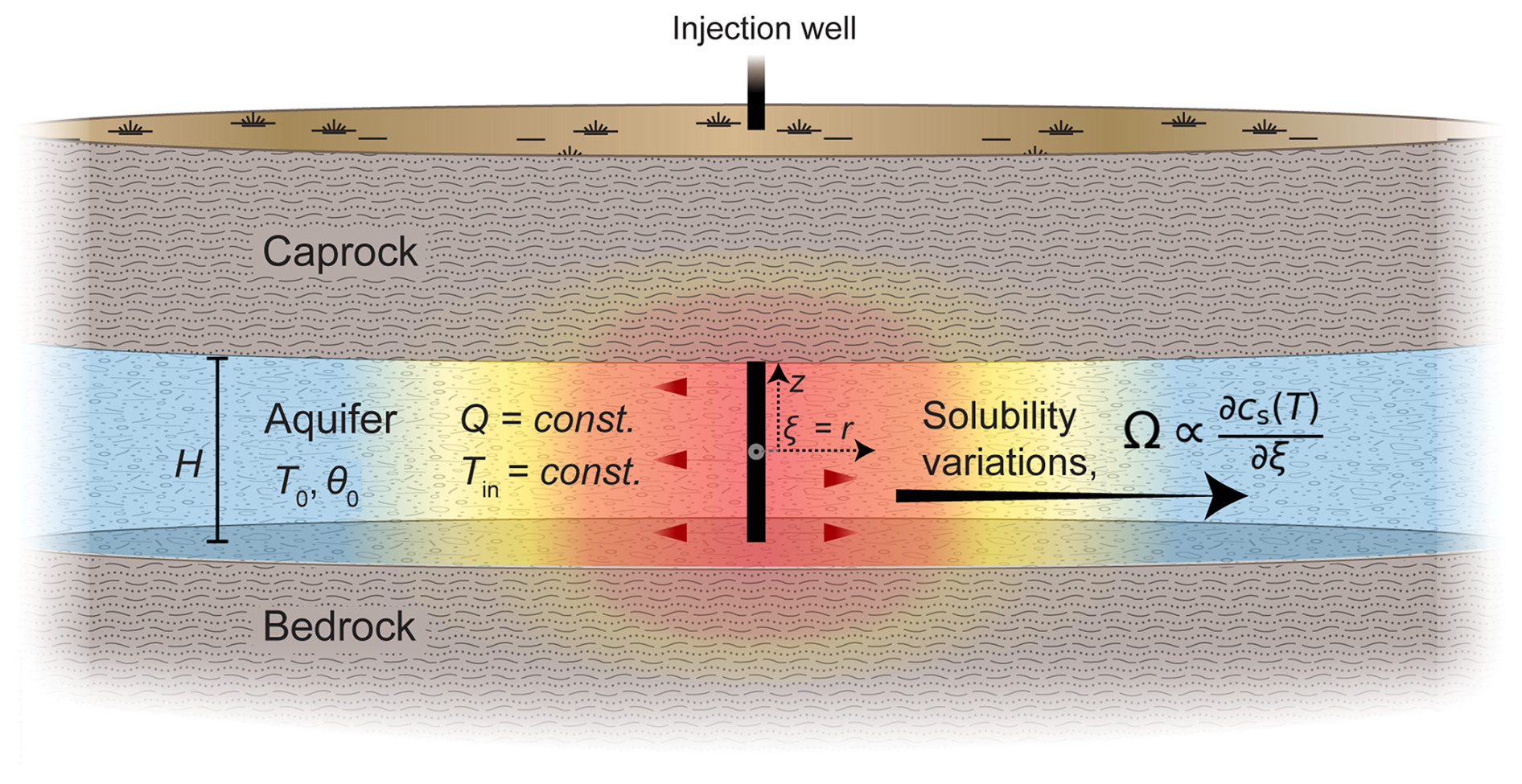
Figure 1 Outline of the reactive Lauwerier problem (RLP) under the equilibrium assumption. Hot (or cold) fluid is injected into an aquifer, confined between impermeable bedrock and caprock, at a steady flow rate, Q, and temperature, T_in. The initial temperature is T₀, and the aquifer thickness is H. Along the flow path, heat from the aquifer conducts through the confining layers. The resulting thermal variations (depicted by color gradients) alter mineral solubility, c_s(T), driving chemical reactions that modify aquifer porosity from its initial value, θ₀. High Damköhler number conditions and the equilibrium assumption are considered. Under these conditions, the reaction rate, Ω, is directly governed by variations in temperature-dependent mineral solubility, $\partial c_{\mathrm{s}}\left(T\right)/\partial \mathit{\xi }$. Here, ξ denotes the horizontal coordinate, either the radial coordinate (r) or the Cartesian coordinate (x), while z denotes the vertical coordinate. The reference point for both ξ and z is the center of the injection well, which serves as the symmetry axis in the radial case (as shown in the sketch) or the symmetry plane in the Cartesian case (modified after Roded et al., 2024b).

2.1 The equilibrium reactive Lauwerier scenario

The Lauwerier problem describes the injection of a hot or cold fluid into a confined aquifer bounded by impermeable bedrock and caprock. Along the horizontal flow path downstream from the injection well, heat is transferred between the aquifer and the confining aquiclude layers, which conduct the heat (Lauwerier, 1955; Stauffer et al., 2014). The horizontal flow direction is described using the ξ coordinate, which can represent either the radial distance (r) in an axisymmetric configuration or the Cartesian coordinate (x) in planar configuration, i.e., ξ=r or x. These represent the two primary geometric settings considered in this study. A schematic overview of this system is provided in Fig. 1, with the nomenclature summarized in Appendix E.

Within the aquifer, thermal variations influence mineral solubility (i.e., saturation concentration, c_s(T)). These solubility changes, in turn, lead to undersaturation and dissolution reactions or, conversely, to supersaturation and precipitation reactions, which modify the aquifer porosity (θ). Porosity changes, whether increases or decreases, depend on thermal changes (heating or cooling) and the solubility nature of the minerals (prograde or retrograde).

In this study, the focus is on conditions where reaction kinetics are fast, the Damköhler number is large (Da > 1), and the local equilibrium assumption holds. Under these conditions, the reaction rate, Ω, as shown in the next section, can be directly calculated from the thermally driven solubility changes in the system; that is, $\mathrm{\Omega }\propto \partial c_{\mathrm{s}}\left(T\right)/\partial \mathit{\xi }$. Hence, such a solution is independent of the specific reaction kinetics involved.

In terms of geometry and hydrogeological scenarios, the radial setting pertains to injection from a single well or accounts for naturally focused flow of deep-origin fluids through faulted or fractured rock, discharging into a shallower aquifer (Craw, 2000; Micklethwaite and Cox, 2006; Roded et al., 2013, 2023; Tripp and Vearncombe, 2004). The planar setting describes injection from a row of wells arranged in a straight-line configuration, as initially formulated by Lauwerier (1955).

2.2 The equilibrium-based approach

The steady-state, solute advection–reaction equation in the aquifer is

$$\begin{array}{}\text{(2)}& \mathrm{0}=-u{\displaystyle \frac{\partial c}{\partial \mathit{\xi }}}-\mathrm{\Omega }(\mathit{\xi },t),\end{array}$$

where ξ is the horizontal coordinate (ξ=r or x), u is the Darcy flux, c is the solute concentration, and Ω(ξ,t) is the reaction rate, which varies in space and time, t (Chaudhuri et al., 2013; Szymczak and Ladd, 2012). In Eq. (2), transient variations are neglected, and the quasi-static approach to reactive flow is applied (see Appendix A and Roded et al., 2024b).

The solute disequilibrium, Λ, is the difference between the dissolved ion concentration, c, and the temperature-dependent solubility (i.e., saturation concentration), c_s(T), viz.,

$$\begin{array}{}\text{(3)}& \mathrm{\Lambda }=c-c_{\mathrm{s}}\left(T\right).\end{array}$$

Equation (2) can then be rewritten as

$$\begin{array}{}\text{(4)}& \mathrm{0}=-u\left[{\displaystyle \frac{\partial \mathrm{\Lambda }}{\partial \mathit{\xi }}}+{\displaystyle \frac{\partial c_{\mathrm{s}}}{\partial \mathit{\xi }}}\right]-\mathrm{\Omega }(\mathit{\xi },t).\end{array}$$

Next, conditions of a high Da number are considered, where reaction rates significantly exceed the rate of advective transport. In this regime, local quasi-equilibrium is maintained along flow paths, and the solute disequilibrium magnitude remains small compared to the overall solubility variation. Specifically, Λ≪Δc_s, where Δc_s denotes the absolute solubility change in the system, Δc_s = |c_s(T_in)−c_s(T₀)|, that is, between solubility at the injection temperature, T_in, and at ambient conditions, T₀.

Under this assumption, the first advective term in Eq. (4) ($u\partial \mathrm{\Lambda }/\partial \mathit{\xi }$) becomes negligible compared to the other terms. The governing equation can thus be approximated as (Andre and Rajaram, 2005; Phillips, 2009, p. 237)

$$\begin{array}{}\text{(5)}& \mathrm{\Omega }(\mathit{\xi },t)=-u{\displaystyle \frac{\partial c_{\mathrm{s}}\left(T\right)}{\partial \mathit{\xi }}}.\end{array}$$

The expression in Eq. (5) provides the THC equilibrium model and demonstrates that, under quasi-equilibrium conditions, the solute concentration, c, closely follows the spatially varying solubility determined by the temperature field, c_s(T). Notably, it shows that in this regime, the solution for the overall reaction rate, Ω(ξ,t), can be independent of the specific reaction kinetics involved and can be calculated from the solubility gradient.

Lastly, it is noted that the current study focuses on the equilibrium assumption and solves the reduced form given in Eq. (5). This contrasts with the preceding work (Roded et al., 2024b), which focused on solving the full form of Eq. (2) (or Eq. 4) under the assumption of first-order kinetics.

2.3 Initial and boundary conditions

The thermal Lauwerier solution incorporates an initial condition of uniform temperature T₀ across the system, along with boundary conditions that specify a constant fluid injection rate at temperature T_in at the injection point (ξ = 0). It is assumed that the thicknesses of the bedrock and caprock, as well as the extent of the aquifer, are infinite.

With respect to the solute transport boundary conditions, the RLP is defined by a constant fluid injection rate at temperature T_in, with an initial solute disequilibrium of Λ = 0 (i.e., saturated fluid) at the inlet (Roded et al., 2024b). In contrast, the equilibrium-approximated solutions derived from Eq. (5) calculate the reaction rate under the assumption that it is proportional to the temperature-driven solubility gradient everywhere. Consequently, as will be shown in the next section, solute transport boundary conditions are not incorporated. This discrepancy is the focus of the analyses in Sect. 3.3.

3 Results: the equilibrium solutions and their applicability

3.1 Derivation of the equilibrium solutions

3.1.1 Axisymmetric (radial) flow

Aquifer temperature

The Lauwerier solutions for the temperature distribution in the aquifer (Lauwerier, 1955; Stauffer et al., 2014) serve as the basis for developing the equilibrium-approximated RLP solutions presented here. These solutions are derived by solving the advective heat transport equation in the aquifer, together with the corresponding conductive heat transfer equation in the confining bedrock and caprock (Eqs. A1–A3 and A6 in Appendix A). The solution for axisymmetric settings is given by

$$\begin{array}{}\text{(6)}& T(r,t)=T_{\mathrm{0}}+\mathrm{\Delta }T\text{erfc}\left[\mathit{\zeta }\right(r,t\left)r^{\mathrm{2}}\right],\end{array}$$

where erfc is the complementary error function, $\mathrm{\Delta }T=T_{\text{in}}-T_{\mathrm{0}}$ is the difference between the injection and ambient aquifer temperatures, and ζ is defined as

$$\begin{array}{}\text{(7)}& \mathit{\zeta }(r,t)={\displaystyle \frac{\mathit{\pi }\sqrt{K_{\mathrm{b}}{C}_{{\mathrm{p}}_{\mathrm{b}}}}}{Q{C}_{{\mathrm{p}}_{\mathrm{f}}}\sqrt{t^{\prime }}}},\end{array}$$

where Q is the total volumetric flow rate, K is the thermal conductivity, and C_p is the volumetric heat capacity, with the subscripts b and f denoting bulk rock and fluid, respectively. The time variable is defined as $t^{\prime }=t-t_{\text{lg}}$, where $t_{\text{lg}}=\mathit{\pi }{r}^{\mathrm{2}}H{C_{\mathrm{p}}}_{\mathrm{b}}/\left({C_{\mathrm{p}}}_{\mathrm{f}}Q\right)$, with H denoting the aquifer thickness (see Fig. 1). Assuming flow is uniform across the vertical thickness (H), the fluid velocity can be calculated from the volumetric flow rate as $u=Q/\left(\mathrm{2}\mathit{\pi }rH\right)$.

The solution of Eq. (6) is valid when $t^{\prime }>\mathrm{0}$ (Stauffer et al., 2014), and it is further assumed here that a sufficiently long time has passed such that $t^{\prime }\approx t$. Specifically, the term t_lg represents a thermal retardation time. It accounts for the delay in the arrival of the thermal front due to advective transport and the thermal energy required to heat the aquifer solid matrix along the flow path (for an analysis of the validity of this assumption, see Roded et al., 2024b).

Additionally, for simplicity, it is assumed that the heat capacities of both the confining rocks and the aquifer are identical. To account for non-uniform heat capacities, an alternative definition of Eq. (6) can be applied (see Eqs. 3.122 and 3.131, along with the corresponding definitions in Stauffer et al., 2014).

Thermally driven solubility changes

The THC equilibrium model in Eq. (5) shows that the reaction rate, Ω(r,t), depends on the thermally driven solubility gradient, $\partial c_{\mathrm{s}}\left(T\right)/\partial r$. Here, the temperature-dependent solubility is calculated using

$$\begin{array}{}\text{(8)}& c_{\mathrm{s}}\left(T\right)=c_{\mathrm{s}}\left(T_{\mathrm{0}}\right)+\mathit{\beta }(T-T_{\mathrm{0}}),\end{array}$$

where the parameter $\mathit{\beta }=\partial c_{\mathrm{s}}/\partial T$. In Eq. (8), a linear relation between c_s and T is assumed, with a constant proportionality factor β, which is positive for minerals of prograde solubility and negative for minerals of retrograde solubility (Corson and Pritchard, 2017; Woods, 2015).

In Eq. (5), the derivative of the solubility can be expanded to $\partial c_{\mathrm{s}}/\partial r$ = $(\partial c_{\mathrm{s}}/\partial T)(\partial T/\partial r)$, and by further substituting the definition β = $\partial c_{\mathrm{s}}/\partial T$, it can be expressed as

$$\begin{array}{}\text{(9)}& \mathrm{\Omega }(r,t)=-u\mathit{\beta }{\displaystyle \frac{\partial T}{\partial r}}.\end{array}$$

The temperature gradient $\partial T/\partial r$ is calculated by substituting the Lauwerier solution (Eq. 6) and performing differentiation, yielding

$$\begin{array}{}\text{(10)}& \mathrm{\Omega }(r,t)=\mathrm{4}u\mathit{\beta }\mathrm{\Delta }T{\displaystyle \frac{\mathit{\zeta }r}{\sqrt{\mathit{\pi }}}}{e}^{(-{\mathit{\zeta }}^{\mathrm{2}}{r}^{\mathrm{4}})},\end{array}$$

which provides the solution for the reaction rate. The evolution of porosity, θ, is described by

$$\begin{array}{}\text{(11)}& {\displaystyle \frac{\partial \mathit{\theta }}{\partial t}}=-{\displaystyle \frac{\mathrm{\Omega }(r,t)}{\mathit{\nu }{c}_{\text{sol}}}},\end{array}$$

where c_sol is the concentration of soluble solid mineral and ν accounts for the stoichiometry of the reaction. Substituting the solution for the reaction rate, Ω (Eq. 10), into Eq. (11) and integrating over time yields the solution for the porosity change:

$$\begin{array}{}\text{(12)}& \mathit{\theta }(r,t)={\mathit{\theta }}_{\mathrm{0}}-\mathrm{4}u\mathrm{\Delta }T{\displaystyle \frac{\mathit{\beta }{\mathit{\zeta }}^{\mathrm{2}}{r}^{\mathrm{3}}t}{\mathit{\upsilon }{c}_{\text{sol}}\sqrt{\mathit{\pi }}}}\mathrm{\Gamma }\left(-{\displaystyle \frac{\mathrm{1}}{\mathrm{2}}},{\mathit{\zeta }}^{\mathrm{2}}{r}^{\mathrm{4}}\right),\end{array}$$

where Γ is the incomplete gamma function.

3.1.2 Planar flow

For the Cartesian case, with injection occurring along a plane, the Lauwerier solution is

$$\begin{array}{}\text{(13)}& T(x,t)=T_{\mathrm{0}}+\mathrm{\Delta }T\text{erfc}\left[\mathit{\omega }\right(x,t\left)x\right],\end{array}$$

where ω is defined as

$$\begin{array}{}\text{(14)}& \mathit{\omega }(x,t)={\displaystyle \frac{\sqrt{K_{\mathrm{b}}{C}_{{\mathrm{p}}_{\mathrm{b}}}}}{H{C}_{{\mathrm{p}}_{\mathrm{f}}}u\sqrt{t^{\prime }}}}\end{array}$$

and $t^{\prime }=t-t_{\text{lg}}$, with t_lg = $x{C_{\mathrm{p}}}_{\mathrm{b}}/\left({C_{\mathrm{p}}}_{\mathrm{f}}u\right)$. Similarly to the radial case, it is assumed here that a sufficiently long time has passed such that the condition $t^{\prime }\approx t$ applies.

Following steps analogous to those in the radial case, the solutions are derived as

$$\begin{array}{}\text{(15)}& \mathrm{\Omega }(x,t)=\mathrm{2}u\mathrm{\Delta }T{\displaystyle \frac{\mathit{\beta }\mathit{\omega }}{\sqrt{\mathit{\pi }}}}{e}^{(-{\mathit{\omega }}^{\mathrm{2}}{x}^{\mathrm{2}})}\end{array}$$

and

$$\begin{array}{}\text{(16)}& \mathit{\theta }(x,t)={\mathit{\theta }}_{\mathrm{0}}-\mathrm{2}u\mathrm{\Delta }T{\displaystyle \frac{\mathit{\beta }{\mathit{\omega }}^{\mathrm{2}}xt}{\mathit{\upsilon }{c}_{\text{sol}}\sqrt{\mathit{\pi }}}}\mathrm{\Gamma }\left(-{\displaystyle \frac{\mathrm{1}}{\mathrm{2}}},{\mathit{\omega }}^{\mathrm{2}}{x}^{\mathrm{2}}\right).\end{array}$$

3.2 Comparison to reference solutions (High-Da)

In this section, the results of the equilibrium solutions are compared with the more general solutions to the RLP model, which will henceforth be referred to as the “reference solutions”. These reference solutions account for far-from-equilibrium conditions and assume surface-controlled reactions and first-order kinetics. The case study considered in the comparison involves a common scenario: dissolution of a fractured carbonate aquifer due to the injection of CO₂-rich hot water and cooling-driven calcite dissolution. First, the results presented by Roded et al. (2024b) for the reference solutions are briefly summarized to facilitate the comparison with the equilibrium solutions. The reference solutions, along with the case study considered here, are detailed in Roded et al. (2024b). The reference solution equations are also provided in Appendix B, and the parameter values used are listed in Appendix D. These values are identical to those in Roded et al. (2024b), including the radial case flow rate (Q = 500 m³ d⁻¹).

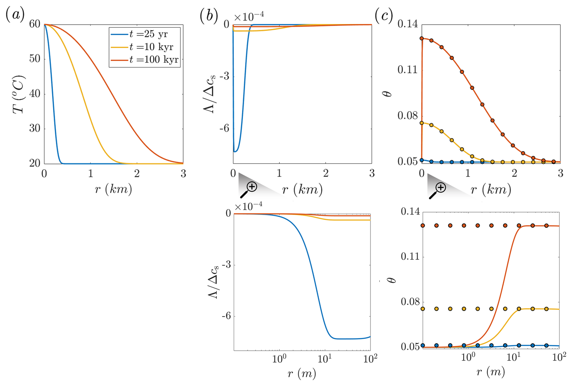
Figure 2 Reference solutions for a case study of carbonate aquifer dissolution by cooling hot water, presented for comparison with the equilibrium solution in a radial flow setting. Panels (a)–(c) show temperature (T), solute disequilibrium (Λ), and porosity (θ) plotted as functions of radial position (r) at different times. The continuous lines represent the Lauwerier solution and the reference solutions (Eqs. 6, B2, and B3), while the circles in panel (c) denote the equilibrium solution (Eq. 12). Magnified panels show solute disequilibrium (Λ) and porosity (θ) near the inlet region. Λ is scaled by the total solubility variation in the system, Δc_s. The equilibrium solution closely matches the reference solution except near the inlet (see magnified panel and text). Quasi-equilibrium conditions are further supported by the small magnitude of Λ.

In Fig. 2, the results of CO₂-rich hot water injection are shown at successive times since the start of injection. These represent both engineering-relevant conditions (t = 25 years) and longer geological timescales (t = 10 and 100 kyr), associated with natural processes such as focused deep-origin flow discharging into a shallower aquifer (Craw, 2000; Roded et al., 2023; Tripp and Vearncombe, 2004). The Lauwerier solution and reference solutions are shown by continuous lines (Eqs. 6, B2, and B3), while the equilibrium solution for the porosity evolution is indicated by circle markers in Fig. 2c (Eq. 12).

During the radial flow within the aquifer, the hot fluid cools by transferring heat into the confining layers, which heat up with time, resulting in the gradual advancement of the thermal front downstream (Fig. 2a). The cooling induces solute disequilibrium (Λ) associated with undersaturation (note that Λ is negative for undersaturation and positive for supersaturation; see Eq. 3). The magnitude of |Λ| in the aquifer is small compared to the absolute solubility change in the system, $\mathrm{|}\mathrm{\Lambda }\mathrm{|}/\mathrm{\Delta }{c}_{\mathrm{s}}\ll$ 1 % (Δc_s = |c_s(T_in)−c_s(T₀)|; see Fig. 2b). The small magnitude of disequilibrium is associated with relatively high CO₂ partial pressure considered (0.03 MPa) and rapid kinetics under these conditions.

Despite its small magnitude, the disequilibrium, Λ, governs the alteration of the aquifer and the evolution of its porosity. Notably, because the water at the inlet is hot and saturated with calcite, c = c_s(T_in), disequilibrium and the reaction rate are zero at the inlet, resulting in no change in porosity (see Fig. 2b and c, along with their magnified views). Disequilibrium (undersaturation) abruptly develops downstream of the injection well, initially forming a small minimum (at r≈ 20 m) before gradually diminishing to zero further downstream.

In accordance with the disequilibrium, the porosity profile sharply increases near the inlet and then gradually decreases downstream (Fig. 2c). Undersaturation and dissolution along the flow path are governed by the interplay of three processes: (I) dissolution, which reduces undersaturation (bringing Λ closer to 0), (II) progressive cooling, which enhances undersaturation, and (III) advection, which transports reaction products (calcium ions) radially outward from the well, sustaining undersaturation. Here, fluid velocity and advection decay with distance, following a $\mathrm{1}/r$ relationship. The transient thermal effect is also evident in the time evolution of the disequilibrium: at early times (t = 25 years), disequilibrium and its gradients are relatively high, but as the thermal front advances and thermal gradients decrease, the disequilibrium curves flatten.

The equilibrium solution matches the reference solution closely and is violated only near the inlet (r < 20 m; Fig. 2c). The agreement between the solutions and the existence of quasi-equilibrium conditions is supported by the small magnitude of the disequilibrium in the reference solution. This is because the equilibrium model assumes Λ = 0 (cf. Eqs. 4 and 5); therefore, a small Λ confirms the validity of this approximation. Consequently, solute disequilibrium provides an effective metric for quantifying the spatial and temporal extent to which the equilibrium assumption holds. This will be used next to further assess the applicability of the equilibrium-approximated solutions (Sect. 3.3).

With respect to the discrepancy near the inlet between the solutions, the injection of hot, saturated water results in no porosity change in the reference solution. In contrast, the equilibrium model, which assumes the reaction rate depends on the temperature gradient alone, does not capture this effect. Particularly, the solute transport boundary condition of inlet saturation (Λ = 0) is not incorporated into the equilibrium-approximated solutions, leading to this discrepancy (referred to hereafter as the “inlet advective discrepancy”).

Under the conditions here, the deviation between the solutions is limited to a very narrow region near the inlet. However, in some cases, locally reduced porosity and permeability can still influence the overall estimation of aquifer permeability (Roded et al., 2024b). While the deviation in these cases can be accounted for by assuming no reaction at the inlet, as will be shown in Sect. 3.3, this cannot capture advective effects that may become significant near the inlet under low Da conditions. It is also noted that in most practical scenarios, the injected fluid is expected to cool slightly during its descent in the well and may therefore already be reactive upon entering the aquifer.

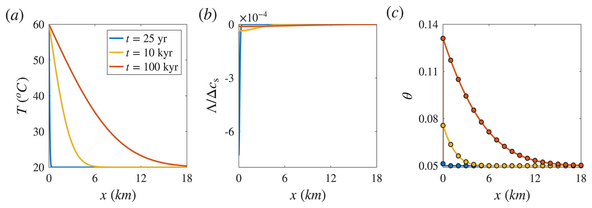
Figure 3 Reference solutions for a case study of carbonate aquifer dissolution by cooling hot water, presented for comparison with the equilibrium solution in a planar flow setting. Panels (a)–(c) show temperature (T), solute disequilibrium (Λ), and porosity (θ) as functions of position (x) at different times. The continuous lines represent the thermal Lauwerier solution and the reference solutions (Eqs. 13, B5, and B6), while the circles in panel (c) denote the equilibrium solution (Eq. 16). Λ is scaled by the total solubility variation in the system, Δc_s. Similar to the radial case, the equilibrium solution closely matches the reference solution except near the inlet. This is also supported by the small magnitude of Λ.

For completeness, Fig. 3 presents results for the same case study shown in Fig. 2 under a planar flow setting, with a fluid velocity of u = 10⁻⁶ m s⁻¹. Similar to the radial case, the equilibrium solution closely matches the reference solution, with deviation occurring only near the inlet (magnification not shown). A key difference from the radial case is that the aquifer is heated over significantly greater distances. This results from the uniform flow velocity and more efficient heat retention in the planar configuration. In contrast, radial flow involves velocity decay with distance, which increases residence time and enhances conductive heat loss to the surrounding rock.

Additionally, in the radial case, the heat source (e.g., an injection well) acts as a source from which hot fluid spreads outward radially. In contrast, the planar configuration can be conceptualized as injection from a distributed source (e.g., a row of wells), generating a uniform planar front. More precisely, under the perfect thermal mixing assumption, the radial case is treated mathematically as a point source, while the planar case is treated as a line source oriented out of the plane. Hence, in the radial case, heat conduction is multidirectional, whereas in the planar case, heat is conducted only in the vertical directions. These differences influence the shape of the temperature profile: in the radial case, effective heating near the injection well and subsequent rapid decay lead to a sigmoidal (or diffusive front-like) profile, whereas in the linear case, there is a decaying profile (cf. Figs. 2a and 3a). These differences are further quantified in Sect. 3.4.

With respect to the results in Figs. 2 and 3, recall that the solutions in Sect. 3.1 rely on the fundamental assumption of spatial uniformity and symmetry in the reactive flow. However, in practical scenarios, dissolution channels (wormholes) may develop at the reaction front (Chadam et al., 1986; Furui et al., 2022; Roded et al., 2021). These wormholes localize reactive flow, creating heterogeneous flow fields that deviate from the assumed symmetry and uniformity. Consequently, the results in Figs. 2 and 3 represent only an average solution and do not capture local flow variations accurately.

Furthermore, the equilibrium solutions were also found to be applicable to the injection of hot, silica-rich water into a sandstone aquifer, where cooling induces supersaturation, silica precipitation, and porosity reduction, as discussed in Roded et al. (2024b) (not presented). In summary, this section validates the equilibrium solutions against the reference solutions and highlights the inlet advective discrepancy, examined next (Sect. 3.3). These findings also demonstrate the broader applicability of the equilibrium solutions across a range of characteristic conditions in natural and applied systems, as further elaborated in the Discussion section.

3.3 Applicability of the RLP equilibrium solutions

This section further examines the applicability of equilibrium-approximated solutions, focusing on the inlet advective discrepancy. This is done by considering lower Da, conditions farther from equilibrium, and changes in the system state over time. Accordingly, a scenario of relatively slow precipitation (β > 0) is considered, using a kinetic rate coefficient nearly 4 orders of magnitude lower (λ = 5 × 10⁻¹⁰ m s⁻¹), while all other conditions remain consistent with Sect. 3.2. This setup is representative, for example, of carbonate mineral precipitation from water of alkaline composition originating in carbonate or mafic rock aquifers (e.g., basaltic formations). Upon reinjection and subsequent heating, the solubility of carbonate phases decreases, promoting CO₂ mineralization through precipitation reactions (Etiope, 2015; Plummer et al., 1978; Steefel and Lichtner, 1998).

Figure 4a presents the results for the reaction rate, Ω, for the reference solution (solid lines; Eq. B3) and the equilibrium solution (dashed lines with circle markers; Eq. 10). The slower kinetics and reduced Da result in a significantly larger deviation compared to the case shown in Figs. 2c and 3c. Note that the results in Figs. 2c and 3c, rather, present the porosity evolution, which reflects the time-integrated behavior of Ω (see Eq. 11).

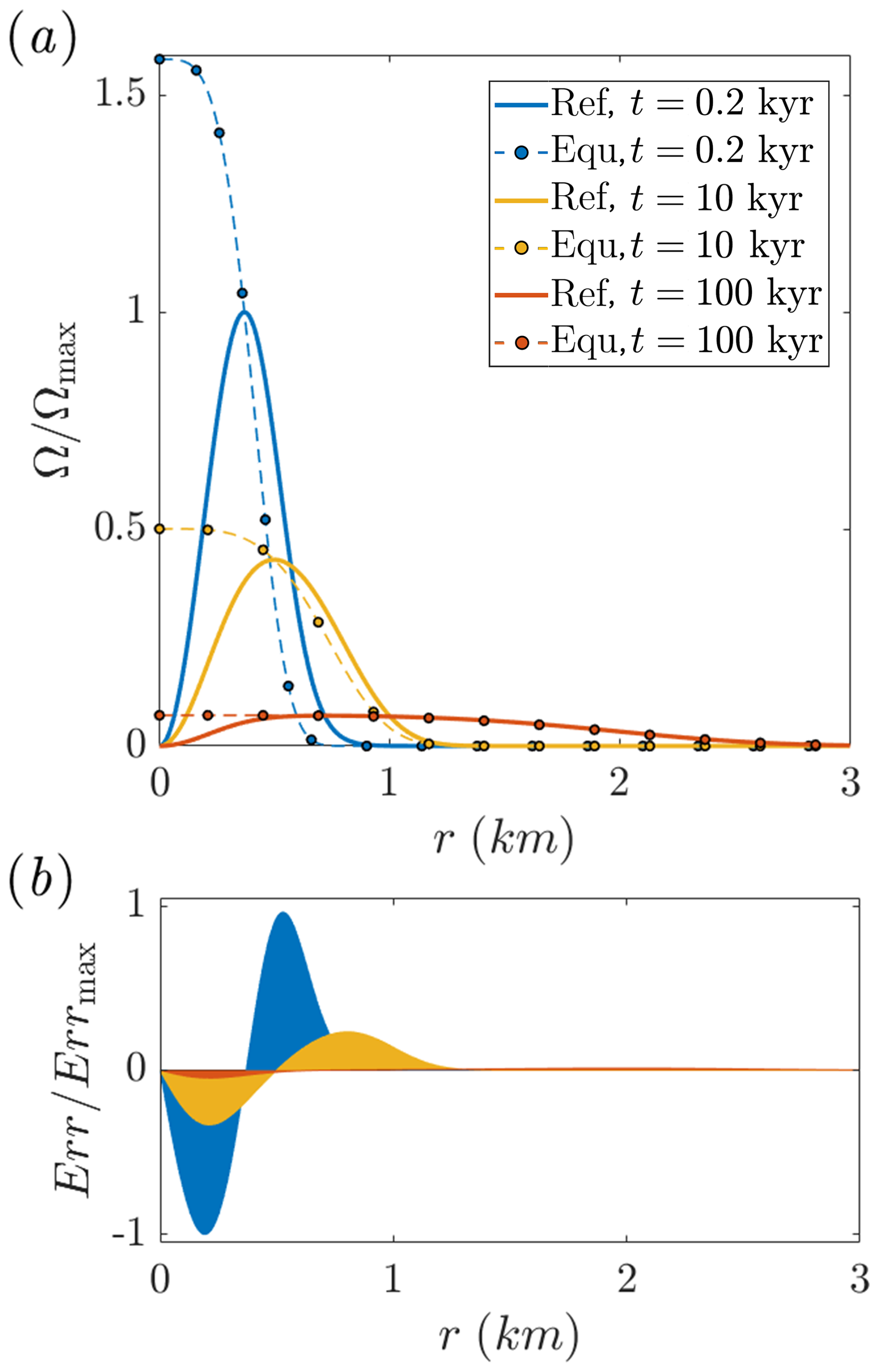
Figure 4 Comparison of the reference and equilibrium solutions over time under low Da conditions. (a) Reaction rate, Ω, as a function of radial position (r) at different times. The continuous lines represent the reference solution (Eq. B3), and dashed lines with circle markers represent the equilibrium solution (Eq. 10), denoted as “Ref” and “Equ” in the legend, respectively. (b) The deviation between the solutions, shown using the local error, Err, is visualized as a shaded region. Err is defined as the radially weighted difference between the solutions (see text for details). Ω and Err are normalized by their maximum values at t = 0.2 kyr, where Ω_max refers to the reference solution.

Significantly, the peak of the reaction rate curve in Fig. 4a is reached further downstream, rather than occurring immediately near the inlet as observed in Figs. 2 and 3. This shift reflects a much more dominant advective effect but still preserves the same general behavior: advection of saturated fluid from the inlet and the progressive buildup of disequilibrium and elevated Ω occur downstream of the injection well. However, in this case, the effect extends over a much greater distance.

Another prominent effect visible in Fig. 4a is the reduction in deviation between the solutions over time. This trend is quantified in Fig. 4b, which shows the weighted local error, defined as the difference between the two solutions and multiplied by the radial perimeter, Err = (Ω_Ref−Ω_Equ)2πr, where the subscripts Ref and Equ denote the reference and equilibrium solutions, respectively.

The Err shaded regions show a progressive decrease and flattening over time. This reduction in Err and the closer approach to equilibrium are attributed to the downstream advancement of the thermal front. As the thermal front advances and extends, the temperature gradients near the inlet become milder (see Fig. 2a). This leads to a decrease in the reaction rate in this region, and the inlet advective discrepancy of the equilibrium model becomes less pronounced (the Supplementary Material (SM) presents results for the planar case, which exhibits the same effects).

As noted in the Introduction, the applicability of the equilibrium model is governed by Da, with quasi-equilibrium conditions expected when Da > 1 (Eq. 1). In the THC equilibrium model and RLP settings, the deviation of the equilibrium solutions, mainly from the local inlet effect, evolves over time and is influenced by thermal dynamics. This observation motivated the derivation of a more specific applicability criterion, presented in Appendix C. This analysis is based on a key feature of quasi-equilibrium behavior: the close alignment of the thermal and reactive fronts in the aquifer, which occurs when Da is high (cf. Fig. 2a and b). This behavior is leveraged to establish a criterion for when the fronts coincide and equilibrium conditions may be assumed. This functional relation, which applies to both planar and radial settings, is given by

$$\begin{array}{}\text{(17)}& \mathrm{1}\gg {\displaystyle \frac{\mathrm{2}}{\sqrt{\mathit{\pi }t}}}\left({\displaystyle \frac{\mathrm{1}}{A_{\mathrm{s}}\mathit{\lambda }}}\right)\left({\displaystyle \frac{\sqrt{K_{\mathrm{b}}{C}_{{\mathrm{p}}_{\mathrm{b}}}}}{H{C}_{{\mathrm{p}}_{\mathrm{f}}}}}\right).\end{array}$$

In accordance with the results in Fig. 4, the criterion shows that the system approaches equilibrium as time progresses (with a proportionality of $t^{-\mathrm{1}/\mathrm{2}}$). The second term in the brackets represents the characteristic reaction timescale, t_R = $\mathrm{1}/A_{\mathrm{s}}\mathit{\lambda }$, which, in agreement with the high Da condition, indicates that a smaller t_R leads to a faster approach to equilibrium. The final term in the brackets captures the ratio of thermal parameters and accounts for the evolution of the temperature gradients. When the confining rock's thermal conductivity (K_b) and heat capacity ($C_{{\mathrm{p}}_{\mathrm{b}}}$) are low, the thermal front advances downstream more rapidly, promoting mild temperature gradients and equilibrium. Similarly, a large product of the aquifer thickness and fluid heat capacity (HC_pf) also facilitates faster thermal front advancement and equilibrium.

Notably, the fluid velocity does not appear in the criterion of Eq. (17). This is attributed to the fact that solute advection enhances disequilibrium (in accordance with the Da criterion), while thermal advection promotes equilibrium by extending and stretching the thermal front. By introducing the characteristic fluid velocity, u_A, into the expression, the criterion in Eq. (17) reproduces the Damköhler number criterion (Eq. 1):

$$\begin{array}{}\text{(18)}& {\displaystyle \frac{l\left(t\right)A_{\mathrm{s}}\mathit{\lambda }}{u_{\mathrm{A}}}}\gg \mathrm{1},\text{where}l\left(t\right)={\displaystyle \frac{\sqrt{\mathit{\pi }}}{\mathrm{2}}}{\displaystyle \frac{u_{\mathrm{A}}H{C}_{{\mathrm{p}}_{\mathrm{f}}}}{\sqrt{K_{\mathrm{b}}{C}_{{\mathrm{p}}_{\mathrm{b}}}}}}{t}^{\mathrm{1}/\mathrm{2}}.\end{array}$$

Thus, this RLP-specific Da criterion incorporates a definition of the local characteristic length scale, l, in terms of time and thermal parameters (dynamic Da). Recall that the length scale l denotes the distance over which substantial temperature variation occurs (e.g., 2 % of the total change) and captures the influence of the thermal field on reactive transport.

The functional criterion in Eqs. (17) and (18), consistent with the results in Fig. 4, indicates that the equilibrium solutions are not applicable as t→0 and are less accurate during the initial stages. Nevertheless, as shown in Fig. 2, the equilibrium-approximated solutions may remain fully valid even at relatively early times. Such behavior is observed under common conditions involving fractured carbonate aquifers and silica precipitation, where the validity extends to timescales of engineering relevance (e.g., t < 25 years).

It should also be recalled that several inherent assumptions in the Lauwerier solution reduce its accuracy during the initial stages (see Appendix A). In addition, for the reactive Lauwerier solution, the assumption of negligible thermal retardation time (t_lg) and the approximation $t^{\prime }\approx t$ further affect the accuracy at early times (see Eqs. 6 and 13). This assumption, which is particularly relevant for the radial case, contributes to the reduced accuracy at early times (e.g., t < 10 years; see Appendix C in Roded et al., 2024b).

3.4 Development of coalesced fronts

As mentioned in the previous section, a key feature of quasi-equilibrium behavior is the close alignment of the thermal and reactive fronts in the aquifer, which occurs when Da is high and reactions dominate over transport. Under these conditions, any disequilibrium induced by thermal changes diminishes rapidly and essentially does not extend downstream of the thermal front, resulting in the coalescence of the fronts. This property is leveraged to infer, in a simple manner, the spatial distribution and temporal advancement of the coalesced fronts using the thermal Lauwerier solutions.

First, we define the thermal fronts' outer-end positions, ξ_F(t), as the furthest distances of thermal perturbation due to the injection at a given time. The thermal perturbation is quantified by ε = $\left(T\right({\mathit{\xi }}_{\mathrm{F}})-T_{\mathrm{0}})/\mathrm{\Delta }T$, where ε is a prescribed small value (ε≪1); here, ε = 0.01. This threshold uniquely determines the position ξ_F(t) at which the temperature perturbation is considered negligible.

Next, rearranging and substituting the definition of ε corresponding to the conditions at the fronts' outer-end positions into the Lauwerier solutions (Eqs. 6 and 13) yield

$$\begin{array}{}\text{(19)}& \mathit{\epsilon }=\text{erfc}\left(a\right),\text{where}a=\left\{\begin{array}{l}\mathit{\zeta }\left(t\right)r_{\mathrm{F}}^{\mathrm{2}},\text{for}\mathit{\xi }=r\\ \mathit{\omega }\left(t\right)x_{\mathrm{F}},\text{for}\mathit{\xi }=x\end{array}\right..\end{array}$$

Here, a is a constant determined by ε, and for ε=0.01, a≈1.8. Then, the fronts' outer-end positions can be expressed as

$$\begin{array}{}\text{(20)}& r_{\mathrm{F}}\left(t\right)=\sqrt{{\displaystyle \frac{a}{\mathit{\zeta }\left(t\right)}}}\text{and}{x}_{\mathrm{F}}\left(t\right)={\displaystyle \frac{a}{\mathit{\omega }\left(t\right)}}.\end{array}$$

Finally, substituting the definitions of ζ and ω (Eqs. 7 and 14) into Eq. (20) gives explicit expressions for the advancement of the coalesced fronts under quasi-equilibrium conditions:

$$\begin{array}{}\text{(21)}& r_{\mathrm{F}}\left(t\right)=\sqrt{{\displaystyle \frac{aQ{C}_{{\mathrm{p}}_{\mathrm{f}}}}{\mathit{\pi }\sqrt{K_{\mathrm{b}}{C}_{{\mathrm{p}}_{\mathrm{b}}}}}}}{t}^{\frac{\mathrm{1}}{\mathrm{4}}},\text{and}{x}_{\mathrm{F}}\left(t\right)={\displaystyle \frac{aH{C}_{{\mathrm{p}}_{\mathrm{f}}}u}{\sqrt{K_{\mathrm{b}}{C}_{{\mathrm{p}}_{\mathrm{b}}}}}}{t}^{\frac{\mathrm{1}}{\mathrm{2}}}.\end{array}$$

These relations provide a simple way to estimate the spatial positions of the coalesced fronts as a function of time using the thermal solutions alone.

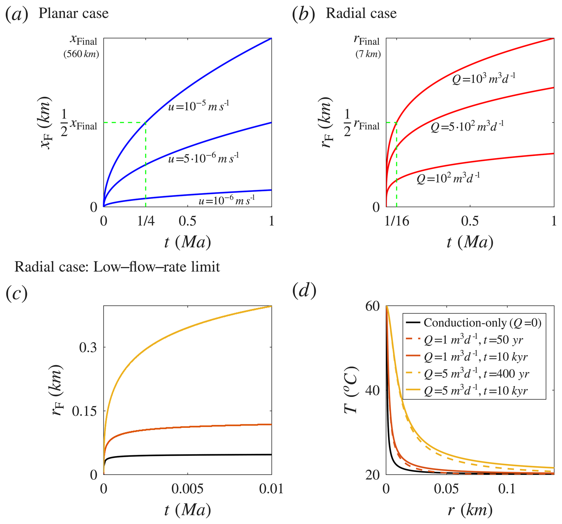
Figure 5 Advancement of the coalesced thermal and reactive fronts over time, x_F(t) and r_F(t), for different velocities (u) and flow rates (Q), respectively. Panels (a) and (b) show results for high flow rates, whereas panels (c) and (d) illustrate the low-flow-rate limit. (a, b) x_F and r_F are calculated using Eq. (21). The green dashed lines illustrate the difference between the radial and planar cases and highlight the greater advancement of the front in the planar case: half of the final extents ($\mathrm{1}/\mathrm{2}{x}_{\text{Final}}$ and $\mathrm{1}/\mathrm{2}{r}_{\text{Final}}$) are reached at $\mathrm{1}/\mathrm{4}$ and $\mathrm{1}/\mathrm{16}$ of the final time, respectively. (c, d) The low-flow-rate limit refers to the radial case where conduction effectively distributes heat. This is analyzed using the solution for the conduction-only setting, representing the limit Q→0 (analytical, black lines), and the results for low flow rates of Q=1 and 5 m³ d⁻¹ (numerical, red and orange, respectively). Panel (c) shows r_F for these cases, whereas panel (d) displays the temperature profiles as a function of radial position, r. The black line in (d) represents the conduction-only quasi-steady-state profile, and the colored dashed and continues lines indicate early and later times, respectively, for each flow rate. The close alignment of the lines demonstrates that the thermal field remains nearly unchanged after the initial stage. For further details on the calculations, refer to the text.

To demonstrate the fronts' advancement, Eq. (21) is used to plot x_F and r_F for three different velocities (u) and flow rates (Q), presented in Fig. 5a and b. This illustrates the decay of the advancement rate over time in both cases: the hot fluid heats the confining rocks as it flows, and the thermal fronts gradually advance downstream. However, front extension overall enhances heat loss to the confining layers, reducing the advancement rate over time and distance.

The key difference between the radial and planar cases, as noted in Sect. 3.2, is clearly reflected in Eq. (21) and the results shown in Fig. 5a and b. The planar case exhibits significantly greater heat retention and a higher advancement rate. This is demonstrated by the green dashed lines in Fig. 5a and b, which indicate that half of the final calculated extent, $\mathrm{1}/\mathrm{2}{x}_{\text{Final}}$, is reached in one-quarter of the final time, while in the radial case, $\mathrm{1}/\mathrm{2}{r}_{\text{Final}}$ is approached after $\mathrm{1}/\mathrm{16}$ of the time. Alternatively, differentiating Eq. (21) with respect to time yields $\partial r_{\mathrm{F}}/\partial t\propto t^{-\mathrm{3}/\mathrm{4}}$ in the radial case, compared to $\partial x_{\mathrm{F}}/\partial t\propto t^{-\mathrm{1}/\mathrm{2}}$ in the planar case.

Another case considered here, shown in Fig. 5c and d, is the low-flow-rate limit in radial geometry, where conduction dominates and effectively distributes heat. This is illustrated using two different approaches: (I) the analytical conduction-only solution, representing the limit Q→0 (black lines), and (II) numerical results for low flow rates (Q=1 and 5 m³ d⁻¹, red and orange curves).

The analytical solution describes a sphere at constant temperature in an infinite medium, modeling heat conducted from the sphere into the surrounding medium. This time-dependent solution converges to a quasi-steady-state temperature profile that remains essentially unchanged over time (Stauffer et al., 2014; see details in the SM). The numerical simulations for low flow rates use equations and settings identical to those of the Lauwerier solution but with an important distinction: they do not assume negligible radial conduction. This simplification makes the Lauwerier solution inadequate under conditions of low flow rates and sharp lateral geothermal gradients (see Appendix A). Further details of the numerical calculations are given in Roded et al. (2023).

Figure 5c shows r_F for the conduction-only case and for Q=1 and 5 m³ d⁻¹ (other parameter values are consistent with Appendix D). Unlike the high-flow-rate planar and radial cases in Fig. 5a and b, the low-flow-rate cases exhibit a more pronounced decrease in the advancement rate over time, reflected in the flattening of the curves. This effect is especially pronounced for the lower flow rate (Q= 1 m³ d⁻¹), which exhibits behavior closer to the conduction-only case, in which the advancement rate essentially levels off as the system approaches the quasi-steady state.

This is more clearly shown in Fig. 5d, which presents the temperature profiles for these cases as a function of the radial position, r. It includes the analytical quasi-steady-state temperature profile (conduction-only case) and numerical profiles at low flow rates shown for two consecutive times. The close alignment of the dashed (early time) and continuous (later time) lines, and their near overlap, demonstrates that the temperature profiles change very little after the early stage. The profiles become nearly stationary over tens to hundreds of years, which is a very brief geological timescale. Hence, even though the front's outer position in the low-flow-rate cases continues to advance slowly, the temperature profile does not change meaningfully. This contrasts with the high-flow-rate cases shown in Figs. 2a and 3a over the long timescale considered.

The results also show effective heat distribution by conduction, with nearly complete cooling occurring within 10–100 m from the inlet, depending on the flow rate. Overall, both the analytical solution for the limit Q→0 and the numerical solutions at low flow rates demonstrate similar heat-transport behavior under these conditions. This low-flow-rate scenario is particularly relevant to natural conditions, which often involve low flow rates and can manifest on the surface as low-flow-rate thermal springs (Garven, 1995; Klimchouk et al., 2017; Roded et al., 2013).

These findings have important implications, suggesting that thermally driven reactive fronts can also become nearly stationary, as will be further discussed in the Discussion section. Lastly, it is important to note that the solutions assume an infinite caprock thickness. However, if the thermal front reaches the surface, greater heat exchange between the aquifer and the caprock is expected, reducing the thermal front's advancement rate and extent (see also Appendix A).

4 Discussion and outlook

4.1 Equilibrium model applicability to hydrothermal systems

Figure 6 presents an illustrative phase diagram distinguishing between conditions where the THC equilibrium model (Eq. 5) is applicable and those far from equilibrium. The diagram is based on the Damköhler number, which represents the ratio between the characteristic timescales of transport and reaction, $\mathit{Da}=t_{\mathrm{A}}/t_{\mathrm{R}}$. The diagonal line marking the transition at Da≫1 (Da_cr) and hotter colors denote higher Da values and conditions closer to equilibrium. As reactivity ($\mathrm{1}/t_{\mathrm{R}}$) increases, the equilibrium model becomes applicable over a wider range of flow velocities, u, or smaller characteristic length scales, l, represented as $\mathrm{1}/t_{\mathrm{A}}=u_{\mathrm{A}}/l$. Here, l represents the local characteristic length scale of thermal and solubility variations and accounts for the thermal field effect on reactive transport, which may vary with time (see Sect. 3.3). Equation (1), which assumes first-order kinetics and presents $\mathit{Da}=l\mathit{\lambda }{A}_{\mathrm{s}}/u_{\mathrm{A}}$, is useful for quantifying different fluid–rock interactions that can be approximated by first-order kinetics.

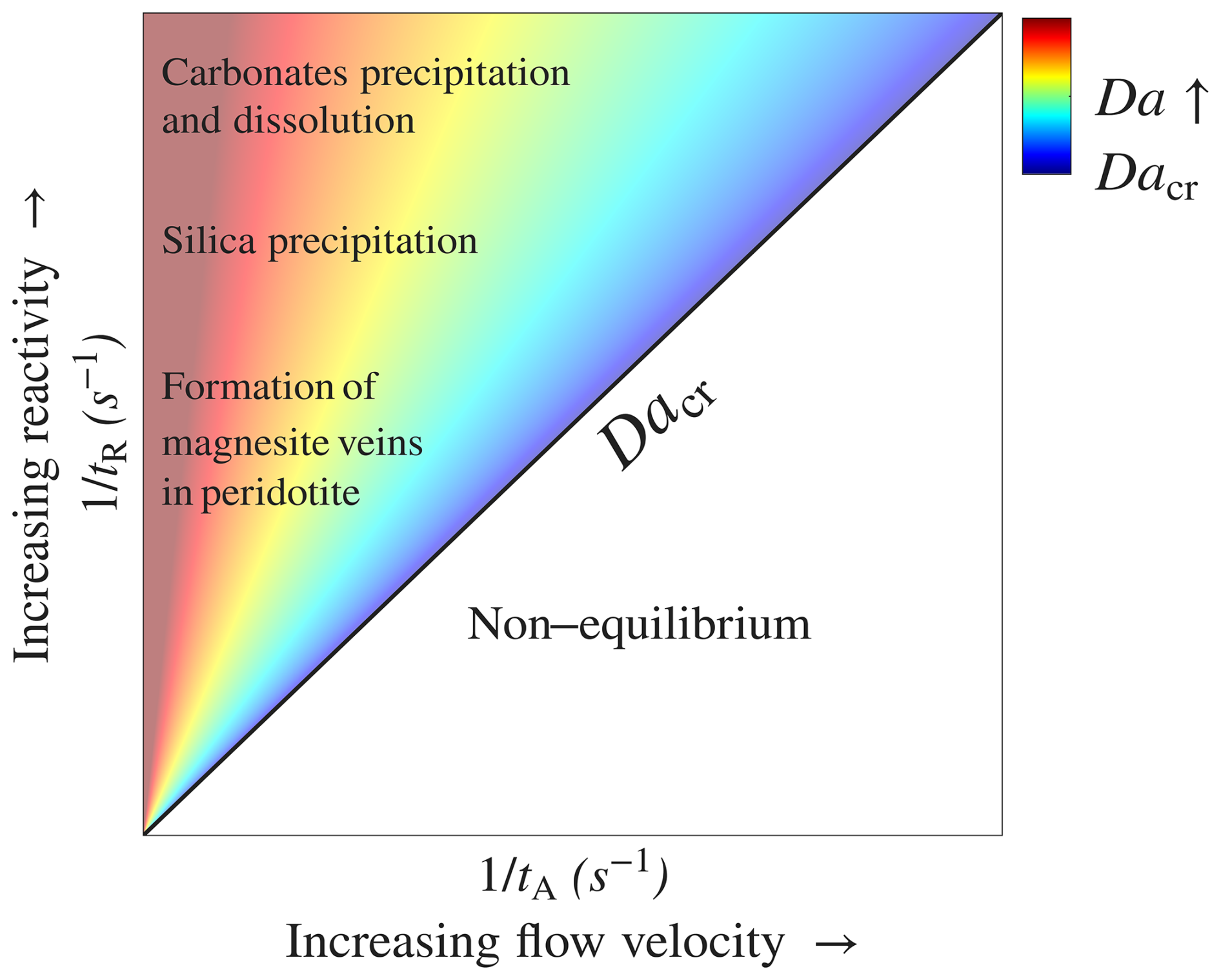
Figure 6 A schematic diagram illustrating the applicability of the THC equilibrium model and the positioning of several notable fluid–rock interaction processes according to their typical reactivity. The diagram is plotted based on the characteristic timescales of reaction and transport that define Da and shows $\mathrm{1}/t_{\mathrm{R}}$ versus $\mathrm{1}/t_{\mathrm{A}}$ ($\mathit{Da}=t_{\mathrm{A}}/t_{\mathrm{R}}$). The equilibrium model can be assumed when Da>Da_cr, with Da_cr defined as a threshold where Da_cr≫1. Da_cr is represented by the diagonal black line on the diagram, with hot colors indicating high Da values and proximity to equilibrium.

Several notable fluid–rock interaction processes are shown on the diagram, positioned according to their characteristic reactivity. At the top are common carbonates, i.e., limestone and dolomite, which typically exhibit high reaction rates and are highly prone to alteration (with values of λ typically ranging from 10⁻⁸ to 10⁻⁴ m s⁻¹ under engineering applications; Dreybrodt et al., 2005; Peng et al., 2015; Plummer et al., 1978).

Silica precipitation is also prevalent in hydrothermal settings (e.g., quartz vein formation and mineral scaling; Glassley, 2014; Huenges and Ledru, 2011; Oliver and Bons, 2001) and is characterized by relatively high reactivity, with a typical rate constant of λ = 5 × 10⁻¹⁰ m s⁻¹ (Rimstidt and Barnes, 1980). In contrast, while non-crystalline silica (amorphous) precipitates relatively quickly, quartz dissolution is typically slower by several orders of magnitude (Rimstidt and Barnes, 1980). An additional interesting behavior associated with quartz occurs at much higher temperatures (e.g., T > 300 °C), which can prevail near magmatic intrusions. At these high temperatures, quartz exhibits retrograde solubility, which switches to prograde solubility upon cooling (Glassley, 2014; Scott and Driesner, 2018).

Importantly, the specific reactive surface area, A_s (L² to L⁻³ of a porous medium), may vary widely across different rock lithologies, and its effect on the applicability of the equilibrium model is comparable to that of kinetics. Specifically, A_s can vary, e.g., from 10⁻¹ m⁻¹ in fractured rock (Deng and Spycher, 2019; Pacheco and Van der Weijden, 2014) to above 10⁵ m⁻¹ for porous medium (Noiriel et al., 2012; Seigneur et al., 2019) and can also evolve during reactive flow (Noiriel, 2015; Seigneur et al., 2019).

The position of these processes on the diagram, supported by calculations in Sect. 3.2, demonstrates the applicability of the equilibrium model even at relatively high flow rates. This is especially significant, as high flow rates are characteristic of applications such as groundwater storage and recovery, aquifer thermal storage, and geothermal reinjection (Diaz et al., 2016; Fleuchaus et al., 2018; Maliva, 2019).

Additional important settings where thermally driven reactions may play a significant role involve mineral carbonation. In particular, this includes the formation of carbonate veins in ultramafic rocks, such as peridotites, by ascending CO₂-rich hydrothermal flow (Kelemen et al., 2011; Menzel et al., 2024). The CO₂-rich fluids first dissolve the rock minerals, primarily olivine. Then, as the pH rises and cation enrichment occurs, carbonate precipitation, primarily magnesite, takes place further along the upward flow path. The rate-limiting step in the mineral carbonation process is commonly suggested to be the relatively slower kinetics of dissolution compared to precipitation (Hänchen et al., 2006; Kaszuba et al., 2013; Kelemen et al., 2019).

The solubility of olivine is retrograde, as evidenced by the exothermic nature of the reaction (Kaszuba et al., 2013; Prigiobbe et al., 2009). Under such conditions, ascending flow along a decreasing geothermal gradient is expected to promote undersaturation. This continued renewal of undersaturation in turn may facilitate the development of an extended, thermally driven dissolution-precipitation front. The typically low rates of ascending hydrothermal flow (e.g., u < 10⁻⁷ m s⁻¹; Garven, 1995), along with characteristic high reaction rates of olivine dissolution at high temperatures (T > 150 °C; Rimstidt, 2015; Rimstidt et al., 2012), suggest that Da can be large. Consequently, mineral carbonation and vein formation can be controlled by thermally driven solubility changes and described by the THC equilibrium model.

4.2 Development of thermally driven reactive fronts in Earth systems

The quasi-equilibrium conditions, characterized by the thermal front's control over the reactive front and their coalescence, allowed examination of their evolution in different settings in Sect. 3.4. A particularly interesting finding is that in radial (or similar) settings, and at relatively low flow rates, a quasi-steady state develops over brief timescales of tens to hundreds of years. Such a cooling process can also produce very steep thermal gradients, as shown in the temperature profile in Fig. 5d, and can cause localized, thermally driven reactive effects. These thermal gradients may be up to 2 orders of magnitude greater than the typical geothermal gradient resulting from Earth's heat flow (e.g., ∼ 0.025 °C m⁻¹; Turcotte and Schubert, 2014).

A relevant example includes hypogenic karst cave formation driven by upwelling hydrothermal flow through a conduit pathway within a fault. This flow discharges and spreads radially in a confined aquifer while cooling rapidly, promoting localized carbonate dissolution around the water inlet (Roded et al., 2023, 2024a). In this case, the results in Fig. 5d suggest that the cave system or alteration front may reach approximately constant final dimensions. These settings may also apply to additional alterations by hypogenic flows and thermal seepages.

Additional relevant settings that can involve coalesced fronts include ascending hydrothermal flow along a decreasing geothermal gradient, leading to cooling and thermally driven reactions. Particularly, as mentioned above (Sect. 4.1), this may induce olivine dissolution followed by mineral carbonation in veins in ultramafic rocks. Alternatively, quartz vein formation dominantly occurs due to cooling along the flow path (Bons, 2000; Sibson et al., 1975). In these settings, coalesced fronts may become stationary as the hot ascending flow alters the background geothermal gradient, producing a modified steady vertical thermal profile (Person et al., 1996; Roded et al., 2013).

In these cases where the coalesced, thermally driven reactive front remains stationary over geological timescales, spatial alteration of the front depends on slower tectonic processes. These tectonic timescales are associated with processes such as erosion, subduction, and orogenic activity. A well-known example is the alteration of the geothermal gradient caused by surface erosion or sediment deposition (Haenel et al., 2012; Turcotte and Schubert, 2014). In response to tectonic changes, the slowly varying subsurface thermal field drives the gradual migration of the reactive front.

4.3 Theoretical modeling outlook

Finally, this study and Roded et al. (2024b) demonstrate the extension of established heat transport solutions to THC-coupled solutions. For future work, the possibility of extending these solutions and approaches in several directions should be investigated. Specifically, it should be examined how the solutions developed can be further extended to address more realistic and complex scenarios. In particular, this includes consideration of more complex kinetic systems involving multiple species and additional or more intricate couplings between variables and parameters.

In such cases, semi-analytical approaches could be especially useful. Due to the quasi-static assumption of reactive flow, the set of equations for the reaction rate (Eqs. 10 and 15) or solute disequilibrium (Eqs. B3 and B6) could potentially be implemented in a semi-analytical, coupled, and iterative manner.

Furthermore, the approach taken here and in Roded et al. (2024b) can be adapted to extend additional thermal solutions to significant thermally driven reactive transport scenarios. Notably, this may be especially practical and feasible under the equilibrium assumption, where thermally driven reactions depend solely on the thermal gradients.

5 Summary and conclusions

In this work, the equilibrium assumption was used to derive thermally driven reactive transport solutions for the RLP (reactive Lauwerier problem) in Cartesian and radial coordinates. The solutions were then validated and analyzed against reference solutions and case studies involving thermally driven reactions of carbonates. In particular, the shortcoming of the equilibrium-approximated solutions associated with the advective boundary condition was analyzed. It was found that as the thermal front advances, inlet temperature gradients become milder and the advective discrepancy becomes less pronounced. This also motivated the derivation of a functional criterion for quasi-equilibrium conditions in the RLP, which reduces to the Damköhler criterion (dynamic Da). The criterion incorporates time and thermal parameters and supports this interpretation.

Following this, a unique feature of quasi-equilibrium conditions – the coalescence of the thermal and reactive fronts – was used to explore their evolution over time. This was examined in both planar and radial settings and under the low-flow-rate limit where conduction effectively distributes heat. The advancement rate in the radial case decays much more rapidly, and, notably, under the low-flow-rate limit, the front can become essentially stationary within a very short period. Additionally, under these conditions, very sharp temperature gradients are created near the inlet, which can induce localized fluid–rock interactions.

The applicability of the THC equilibrium model for notable fluid–rock interaction processes was then discussed. These include sedimentary reservoir evolution through reactions involving silica and carbonates, as well as natural mineral carbonation in ultramafic rocks. These processes were positioned on a phase diagram based on the Damköhler number, illustrating the applicability of the equilibrium model.

Notably, the theoretical approach used here – extending established heat-transport solutions to thermally driven reactive transport – may also be applicable to other important Earth system scenarios. Finally, it is emphasized that because thermally driven reactive fronts often become essentially stationary within a short period, their evolution is governed by geological processes. These processes, such as tectonics or surface erosion and deposition, operate on much longer timescales.

Appendix A: Underlying assumptions and equations of the equilibrium RLP

This appendix describes the main assumptions of the RLP under the equilibrium assumption. It follows the main presentation from Roded et al. (2024b) and extends it to account for the quasi-equilibrium conditions considered in this study. First, the main assumptions are detailed, followed by a comprehensive overview of the basic conservation equations.

A1 Main model assumptions

The thermal Lauwerier (Lauwerier, 1955) solution involves several simplifying assumptions. These include neglecting the initial geothermal gradient and assuming that the basal geothermal heat flux is negligible compared to the heat supplied by the injected fluid. The aquifer is also assumed to be situated at depth, preventing heat from being transferred to the surface; otherwise, there would be greater heat exchange between the aquifer and the caprock. This assumption also depends on the timescale of interest: the thermal front, which rises over time, may not extend to the surface on a short timescale. However, over a longer period, it may transfer heat to the surface, which can be calculated using the characteristic timescale of conduction t_C ($t_{\mathrm{C}}=l_{\mathrm{C}}^{\mathrm{2}}/{\mathit{\alpha }}_{\mathrm{b}}$, where l_C accounts for the characteristic length scale of conduction and α_b is the thermal diffusivity).

In the confining layers, heat is transferred solely through conduction in the vertical direction (z), while neglecting lateral (ξ) heat conduction. This assumption restricts the model's applicability to cases with high injected fluid fluxes, where mild lateral temperature gradients evolve. To evaluate the validity of this assumption, a thermal Péclet number is employed, which compares heat advection in the aquifer to lateral heat conduction in the confining layers: ${\mathit{Pe}}_{\mathrm{T}}=u_{\mathrm{A}}l/{\mathit{\alpha }}_{\mathrm{b}}$, where l is a length scale at which substantial temperature variation occurs (e.g., the distance corresponding to 2 % of the total temperature change, ΔT). A posteriori inspection confirms that Pe_T≫1 beyond the initial moments under all conditions considered here. Moreover, after a very short initial phase, the length scale l should exceed the vertical dimension of the aquifer, H, where complete thermal mixing is assumed (l≫H). This assumption may not hold if a thick aquifer (i.e., large H) is considered, and significant vertical temperature gradients are expected to develop.

Additionally, thermal and solute dispersions within the aquifer are neglected, as both thermal (Pe_T) and solute (Pe_s) Péclet numbers are assumed to be large. Properties of the fluid and solid phases, such as density and thermal conductivity, are assumed to be constant and temperature-independent. Finally, it is assumed that Da>1, making the equilibrium assumption applicable. As a result, reaction rates are essentially independent of kinetics and reactive surface area, as demonstrated in Sect. 2.2 of the main text.

A2 The basic conservation equations

Heat transport:

Here, the basic conservation equations that underlie the Lauwerier solutions (Eqs. 6 and 13) and the THC equilibrium model (Eq. 5) are presented. More general versions of the conservation equations are provided in Roded et al. (2024b). In what follows, the radial case (ξ=r) is considered first, followed by the planar flow case and Cartesian coordinates (ξ=x).

Assuming that heat transfer in the radial direction, r, is negligible, the heat equation in the bedrock and caprock confining the aquifer is

$$\begin{array}{}\text{(A1)}& {\displaystyle \frac{\partial T}{\partial t}}={\mathit{\alpha }}_{\mathrm{b}}{\displaystyle \frac{{\partial }^{\mathrm{2}}T}{\partial z^{\mathrm{2}}}},\text{for}\left\{\begin{array}{l}z\le -\frac{H}{\mathrm{2}}\\ z\ge \frac{H}{\mathrm{2}}\end{array}\right.,\end{array}$$

where T denotes temperature, t is time, z is the vertical coordinate originating at the center of the injection well, and H denotes the aquifer thickness (see Fig. 1). The thermal diffusivity is given by ${\mathit{\alpha }}_{\mathrm{b}}=K_{\mathrm{b}}/C_{{\mathrm{p}}_{\mathrm{b}}}$, where the subscript b denotes bulk rock, K is the thermal conductivity, and C_p is the volumetric heat capacity (Chen and Reddell, 1983; Stauffer et al., 2014).

Assuming that heat transport in the aquifer is dominated by advection and that perfect mixing prevails in the transverse direction (z), a “depth-averaged” heat transport equation can be derived for the aquifer domain:

$$\begin{array}{}\text{(A2)}& \begin{array}{rl}{C}_{{\mathrm{p}}_{\mathrm{b}}}H{\displaystyle \frac{\partial T}{\partial t}}=& -C_{{\mathrm{p}}_{\mathrm{f}}}H{\displaystyle \frac{\mathrm{1}}{r}}{\displaystyle \frac{\partial \left(ruT\right)}{\partial r}}-\mathit{n}\cdot \mathrm{\Theta }(r,t),\\ & \text{for}-{\displaystyle \frac{H}{\mathrm{2}}}\le z\le {\displaystyle \frac{H}{\mathrm{2}}},\end{array}\end{array}$$

where subscript f denotes fluid and u is the Darcy flux, assumed to be uniform along the z direction, which is calculated from the total volumetric flow rate, Q, using $u\left(r\right)=Q/\left(H\mathrm{2}\mathit{\pi }r\right)$ (Andre and Rajaram, 2005; Lauwerier, 1955). The function Θ accounts for the heat exchange between the aquifer and the confining bedrock and caprock, calculated using Fourier's law, assuming continuous temperature at the interfaces:

$$\begin{array}{}\text{(A3)}& \mathrm{\Theta }=-\mathrm{2}{K}_{\mathrm{b}}{\displaystyle \frac{\partial T}{\partial z}}{\mathrm{|}}_{z=\frac{H}{\mathrm{2}},-\frac{H}{\mathrm{2}}}.\end{array}$$

The factor of 2 accounts for both the bedrock and caprock (Stauffer et al., 2014). In Eq. (A2), n represents a unit vector directed outward from the aquifer and perpendicular to the interface between the aquifer and the bedrock or caprock. This orientation ensures that, e.g., in the case of a warmer aquifer, the upward and downward heat fluxes constitute a heat sink.

Reactive transport:

The solute advection–reaction equation in the aquifer is

$$\begin{array}{}\text{(A4)}& \mathrm{0}=-u{\displaystyle \frac{\partial c}{\partial r}}-\mathrm{\Omega }(r,t),\text{for}-{\displaystyle \frac{H}{\mathrm{2}}}\le z\le {\displaystyle \frac{H}{\mathrm{2}}},\end{array}$$

where c is the solute concentration and Ω is the reaction rate (Chaudhuri et al., 2013; Szymczak and Ladd, 2012). Note that the transient and dispersivity terms in Eq. (A4) are neglected, with the latter being omitted due to the assumption of Pe_s≫1. The justification for neglecting the transient term and invoking the quasi-static approximation in the derivation of Eq. (A4) lies in the separation of timescales between the relaxation of solute concentration (t_A), heat conduction (t_C) in the confining rocks, and mineral alteration (for an in-depth analysis and discussion, see Roded et al., 2024b, and as well, e.g., Bekri et al., 1995; Ladd and Szymczak, 2017; Lichtner, 1991; Roded et al., 2020).

Using the reaction rate, the change in porosity, θ, can be calculated as

$$\begin{array}{}\text{(A5)}& {\displaystyle \frac{\partial \mathit{\theta }}{\partial t}}=-{\displaystyle \frac{\mathrm{\Omega }}{\mathit{\nu }{c}_{\text{sol}}}},\text{for}-{\displaystyle \frac{H}{\mathrm{2}}}\le z\le {\displaystyle \frac{H}{\mathrm{2}}}.\end{array}$$

Here, c_sol represents the concentration of soluble solid mineral, and ν accounts for the stoichiometry of the reaction. For planar flow and Cartesian coordinates, r can be substituted with x in the equations above, while Eq. (A2) takes the following form:

$$\begin{array}{}\text{(A6)}& \begin{array}{rl}{C}_{{\mathrm{p}}_{\mathrm{b}}}H{\displaystyle \frac{\partial T}{\partial t}}=& -u{C}_{{\mathrm{p}}_{\mathrm{f}}}H{\displaystyle \frac{\partial T}{\partial x}}-\mathit{n}\cdot \mathrm{\Theta }(x,t),\\ & \text{for}-{\displaystyle \frac{H}{\mathrm{2}}}\le z\le {\displaystyle \frac{H}{\mathrm{2}}}.\end{array}\end{array}$$

The above set of heat transport equations underlies the development of the thermal Lauwerier solutions presented in Sect. 3.1 (Eqs. 6 and 13). Section 2.2 of the main text provides the derivation of the equilibrium-approximated form of Eq. (A4), which is used to obtain the equilibrium-approximated solutions developed in this study.

Appendix B: RLP solutions

B1 Radial case

The solution to the RLP for solute disequilibrium in the radial case is given by

$$\begin{array}{}\text{(B1)}& \mathrm{\Lambda }=\mathrm{\Delta }T\mathit{\beta }{e}^{\left(\frac{{\mathit{\eta }}^{\mathrm{2}}}{\mathrm{4}{\mathit{\zeta }}^{\mathrm{2}}}-\mathit{\eta }{r}^{\mathrm{2}}\right)}\left(\text{erf}\left[\mathit{\zeta }{r}^{\mathrm{2}}-{\displaystyle \frac{\mathit{\eta }}{\mathrm{2}\mathit{\zeta }}}\right]+\text{erf}\left[{\displaystyle \frac{\mathit{\eta }}{\mathrm{2}\mathit{\zeta }}}\right]\right),\end{array}$$

where $\mathit{\eta }=\mathit{\pi }H{A}_{\mathrm{s}}\mathit{\lambda }/Q$ and the definition of ζ is given in Eq. (7).

A closed-form expression for the temporal and spatial evolution of porosity, θ, is given by

$$\begin{array}{}\text{(B2)}& \begin{array}{rl}\mathit{\theta }(r,t)=& {\mathit{\theta }}_{\mathrm{0}}+\mathrm{4}{\displaystyle \frac{{\mathit{\zeta }}^{\mathrm{2}}t}{{\mathit{\eta }}^{\mathrm{2}}}}{\displaystyle \frac{\mathit{\lambda }{A}_{\mathrm{s}}\mathrm{\Delta }T\mathit{\beta }}{\mathit{\nu }{c}_{\text{sol}}}}\left(-e^{\mathit{\eta }/\mathrm{4}\left(\frac{\mathit{\eta }}{{\mathit{\zeta }}^{\mathrm{2}}}-\mathrm{4}{r}^{\mathrm{2}}\right)}\right.\\ & \times \left(\text{erf}\left[\mathit{\zeta }{r}^{\mathrm{2}}-{\displaystyle \frac{\mathit{\eta }}{\mathrm{2}\mathit{\zeta }}}\right]+\text{erf}\left[{\displaystyle \frac{\mathit{\eta }}{\mathrm{2}\mathit{\zeta }}}\right]\right)\\ & +{\displaystyle \frac{\mathit{\eta }}{\mathit{\zeta }\sqrt{\mathit{\pi }}}}{e}^{-\mathit{\eta }{r}^{\mathrm{2}}}+\text{erf}\left[\mathit{\zeta }{r}^{\mathrm{2}}\right](\mathrm{1}-\mathit{\eta }{r}^{\mathrm{2}})\\ & \left.-{\displaystyle \frac{\mathit{\eta }}{\mathit{\zeta }\sqrt{\mathit{\pi }}}}{e}^{-{\mathit{\zeta }}^{\mathrm{2}}{r}^{\mathrm{4}}}+\mathit{\eta }{r}^{\mathrm{2}}-\mathrm{1}\right).\end{array}\end{array}$$

For efficient computation and preventing integer overflow, an approximate solution of Eq. (B1) is developed using the first-order asymptotic expansion of erfc:

$$\begin{array}{}\text{(B3)}& \mathrm{\Lambda }={\displaystyle \frac{\mathrm{\Delta }T\mathit{\beta }}{\sqrt{\mathit{\pi }}}}{e}^{(-\mathit{\eta }{r}^{\mathrm{2}})}\left({\displaystyle \frac{{\mathrm{e}}^{(\mathit{\eta }{r}^{\mathrm{2}}-{\mathit{\zeta }}^{\mathrm{2}}{r}^{\mathrm{4}})}}{\frac{\mathit{\eta }}{\mathrm{2}\mathit{\zeta }}-\mathit{\zeta }{r}^{\mathrm{2}}}}-{\displaystyle \frac{\mathrm{2}\mathit{\zeta }}{\mathit{\eta }}}\right).\end{array}$$

B2 Planar case

For the planar case, the corresponding solutions are given by

$$\begin{array}{}\text{(B4)}& \mathrm{\Lambda }=\mathrm{\Delta }T\mathit{\beta }{e}^{\left(\frac{{\mathit{\sigma }}^{\mathrm{2}}}{\mathrm{4}{\mathit{\omega }}^{\mathrm{2}}}-\mathit{\sigma }x\right)}\left(\text{erf}\left[\mathit{\omega }x-{\displaystyle \frac{\mathit{\sigma }}{\mathrm{2}\mathit{\omega }}}\right]+\text{erf}\left[{\displaystyle \frac{\mathit{\sigma }}{\mathrm{2}\mathit{\omega }}}\right]\right)\end{array}$$

and

$$\begin{array}{}\text{(B5)}& \begin{array}{rl}\mathit{\theta }(x,t)=& {\mathit{\theta }}_{\mathrm{0}}+\mathrm{4}{\displaystyle \frac{{\mathit{\omega }}^{\mathrm{2}}t}{{\mathit{\sigma }}^{\mathrm{2}}}}{\displaystyle \frac{\mathit{\lambda }{A}_{\mathrm{s}}\mathrm{\Delta }T\mathit{\beta }}{\mathit{\nu }{c}_{\text{sol}}}}\left(-e^{\mathit{\sigma }/\mathrm{4}\left(\frac{\mathit{\sigma }}{{\mathit{\omega }}^{\mathrm{2}}}-\mathrm{4}x\right)}\right.\\ & \times \left(\text{erf}\left[\mathit{\omega }x-{\displaystyle \frac{\mathit{\sigma }}{\mathrm{2}\mathit{\omega }}}\right]+\text{erf}\left[{\displaystyle \frac{\mathit{\sigma }}{\mathrm{2}\mathit{\omega }}}\right]\right)\\ & +{\displaystyle \frac{\mathit{\sigma }}{\mathit{\omega }\sqrt{\mathit{\pi }}}}{e}^{-\mathit{\sigma }x}+\text{erf}\left[\mathit{\omega }x\right](\mathrm{1}-\mathit{\sigma }x)\\ & \left.-{\displaystyle \frac{\mathit{\sigma }}{\mathit{\omega }\sqrt{\mathit{\pi }}}}{e}^{-{\mathit{\omega }}^{\mathrm{2}}{x}^{\mathrm{2}}}+\mathit{\sigma }x-\mathrm{1}\right).\end{array}\end{array}$$

An approximate expression for Eq. (B4) is given by

$$\begin{array}{}\text{(B6)}& \mathrm{\Lambda }={\displaystyle \frac{\mathrm{\Delta }T\mathit{\beta }}{\sqrt{\mathit{\pi }}}}{e}^{(-\mathit{\sigma }x)}\left({\displaystyle \frac{{\mathrm{e}}^{(\mathit{\sigma }x-{\mathit{\omega }}^{\mathrm{2}}{x}^{\mathrm{2}})}}{\frac{\mathit{\sigma }}{\mathrm{2}\mathit{\omega }}-\mathit{\omega }x}}-{\displaystyle \frac{\mathrm{2}\mathit{\omega }}{\mathit{\sigma }}}\right).\end{array}$$

Here, $\mathit{\sigma }=A_{\mathrm{s}}\mathit{\lambda }/u$, and the definition of ω is given in Eq. (14).

To prevent integer overflow errors, Eqs. (B3) and (B6) are used to calculate the undersaturation profiles shown in Figs. 2b and 3b and the reaction rate profiles in Fig. 4a. These expressions are also employed in the iterative numerical solution to obtain the porosity profiles at t = 100 kyr, shown in Figs. 2c and 3c. Prior validation confirmed the accuracy of the approximate solutions (Eqs. B3 and B6; Roded et al., 2024b).

Appendix C: Derivation of the applicability criterion

In this appendix, the derivation of the applicability criterion shown in Sect. 3.3 is presented. This criterion provides a functional relationship between key parameters, variables, and the system equilibrium state in RLP settings. The derivation of the criterion leverages a key feature of the quasi-equilibrium regime: the coalescence of the thermal and reactive fronts in the aquifer, which occurs when Da is high (compare the curves in Fig. 2a and b). In this regime, reactions dominate over transport, and thermally induced disequilibrium dissipates rapidly, essentially not extending downstream of the thermal front.

It is noted that even when the fronts coincide downstream, far-from-equilibrium conditions may still persist upstream. This is observed in the results of Fig. 4, where the equilibrium solution (which aligns with the thermal front) and the reference solution closely match downstream at later times but diverge upstream. Nonetheless, the derived functional relationships offer useful guidance.

First, the thermal front's outer-end position, ξ_F(t), is defined as the furthest distance of thermal perturbation due to the injection at a given time. The thermal perturbation is quantified by ε = ($T\left({\mathit{\xi }}_{\mathrm{F}}\right)-T_{\mathrm{0}})/\mathrm{\Delta }T$, where ε is a prescribed small value (ε≪1); here, ε = 0.01. Here, we consider the radial case (ξ_F=r_F), though applying the same steps to the planar case equations yields the same result.

Rearranging and substituting the definition of ε into the Lauwerier solution (Eq. 6) yield

$$\begin{array}{}\text{(C1)}& \mathit{\epsilon }=\text{erfc}\left(a\right),\text{where}a=\mathit{\zeta }\left(t\right)r_{\mathrm{F}}^{\mathrm{2}},\end{array}$$

where a is a constant, and for ε = 0.01, a≈ 1.8. Then, r_F can be expressed as

$$\begin{array}{}\text{(C2)}& r_{\mathrm{F}}=\sqrt{{\displaystyle \frac{a}{\mathit{\zeta }\left(t\right)}}}.\end{array}$$

Next, an approximate form of the reference solution for disequilibrium is used (Eq. B3 in Appendix B; Roded et al., 2024b). The reasoning for using a far-from-equilibrium-based solution, even though the equilibrium model strictly assumes Λ = 0 (cf. Eqs. 4 and 5), is that small Λ confirms the validity of this approximation. Therefore, solute disequilibrium serves as a metric to quantify the spatial and temporal extent over which the equilibrium assumption is valid.

Assuming quasi-equilibrium at the front's outer-end position, r_F, and applying the condition $\mathit{\epsilon }\ge \mathrm{\Lambda }/\mathrm{\Delta }{c}_{\mathrm{s}}$, where Δc_s denotes the solubility change in the system, $\mathrm{\Delta }{c}_{\mathrm{s}}=c_{\mathrm{s}}\left(T_{\text{in}}\right)-c_{\mathrm{s}}\left(T_{\mathrm{0}}\right)$, which here may be positive or negative, Eq. (B3) becomes

$$\begin{array}{}\text{(C3)}& \mathit{\epsilon }\ge {\displaystyle \frac{\mathrm{\Delta }T}{\mathrm{\Delta }{c}_{\mathrm{s}}}}{\displaystyle \frac{\mathit{\beta }}{\sqrt{\mathit{\pi }}}}{e}^{\left(-\mathit{\eta }{r}_{\mathrm{F}}^{\mathrm{2}}\right)}\left({\displaystyle \frac{{\mathrm{e}}^{\left(\mathit{\eta }{r}_{\mathrm{F}}^{\mathrm{2}}-{\mathit{\zeta }}^{\mathrm{2}}{r}_{\mathrm{F}}^{\mathrm{4}}\right)}}{\frac{\mathit{\eta }}{\mathrm{2}\mathit{\zeta }}-\mathit{\zeta }{r}_{\mathrm{F}}^{\mathrm{2}}}}-{\displaystyle \frac{\mathrm{2}\mathit{\zeta }}{\mathit{\eta }}}\right).\end{array}$$

Next, applying a few more steps by substituting the definition from Eq. (C2), neglecting early times, and assuming high Da and η≫ζ, Eq. (C3) can be simplified to

$$\begin{array}{}\text{(C4)}& \mathit{\epsilon }\ge {\displaystyle \frac{\mathrm{\Delta }T}{\mathrm{\Delta }{c}_{\mathrm{s}}}}{\displaystyle \frac{\mathit{\beta }}{\sqrt{\mathit{\pi }}}}{\displaystyle \frac{\mathrm{2}\mathit{\zeta }}{\mathit{\eta }}}.\end{array}$$

Noting that $\mathit{\beta }=\mathrm{\Delta }{c}_{\mathrm{s}}/\mathrm{\Delta }T$ and explicitly substituting the parameters using Eq. (7) and $\mathit{\eta }=\mathit{\pi }H{A}_{\mathrm{s}}\mathit{\lambda }/Q$, Eq. (C4) becomes

$$\begin{array}{}\text{(C5)}& \mathrm{1}\gg {\displaystyle \frac{\mathrm{2}}{\sqrt{\mathit{\pi }t}}}\left({\displaystyle \frac{\mathrm{1}}{A_{\mathrm{s}}\mathit{\lambda }}}\right)\left({\displaystyle \frac{\sqrt{K_{\mathrm{b}}{C}_{{\mathrm{p}}_{\mathrm{b}}}}}{H{C}_{{\mathrm{p}}_{\mathrm{f}}}}}\right),\end{array}$$

where A_s is the specific reactive area [L⁻¹] and λ is the kinetic reaction rate coefficient of the first-order reaction [L T⁻¹]. Equation (C5) defines the conditions under which the thermal and reactive fronts coincide and provides a functional relationship to the equilibrium state in RLP settings. As shown in the main text, this criterion reduces to the Da criterion (Eq. 1) but further defines the local characteristic length scale, l, through time and thermal parameters (dynamic Da) in RLP settings.

Appendix D: Parameter values

Table D1 Parameter values used in the simulation in Sect. 3.2.

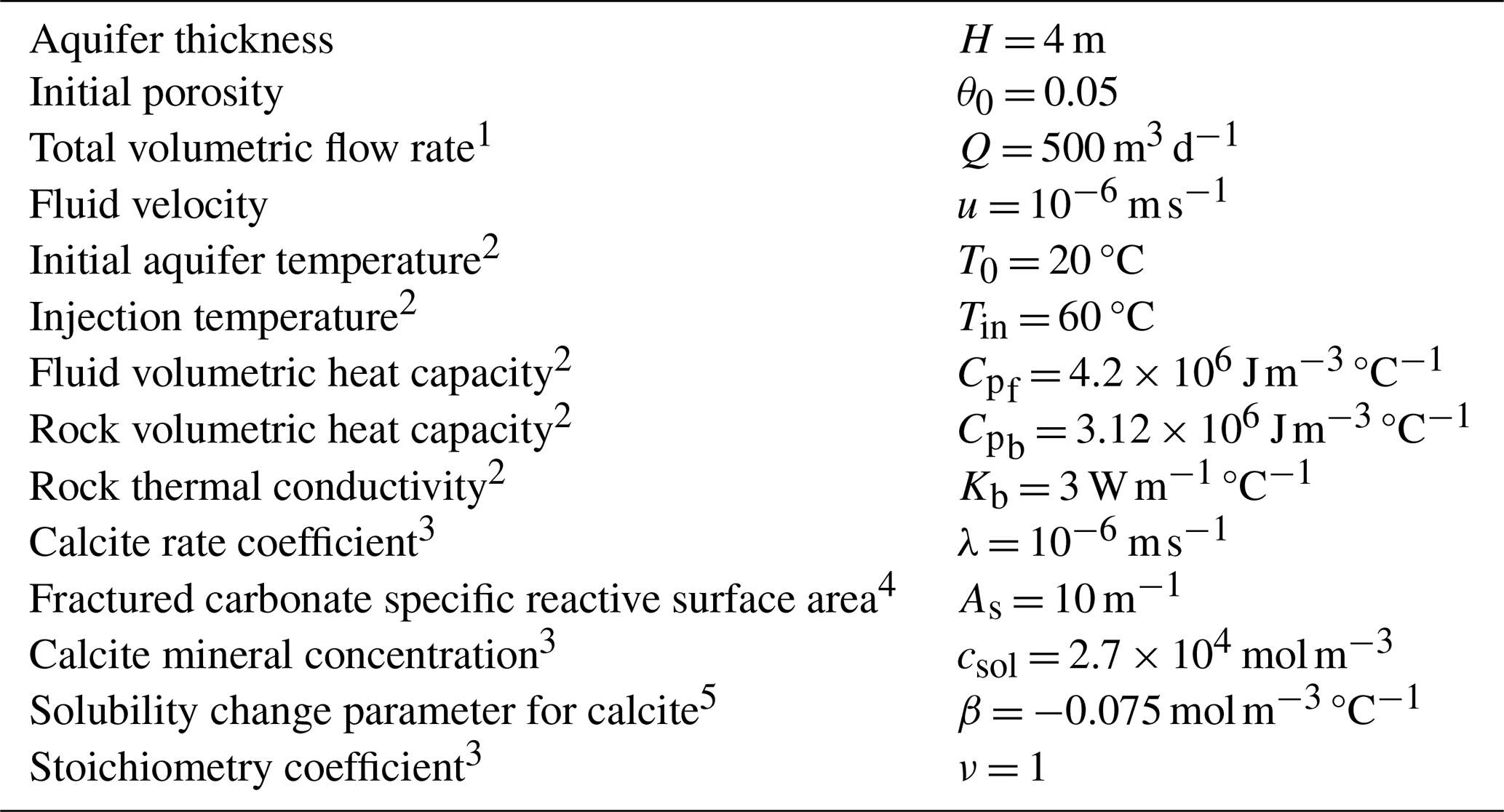
¹ – Glassley (2014); ² – Huenges and Ledru (2011); ³ – Palmer (1991); ⁴ – see Sect. 4.1; ⁵ – Roded et al. (2023).

Appendix E: Nomenclature

Table E1 List of symbols.