Multi-fidelity model assessment of climate change impacts on river water temperatures and thermal extremes and potential effects on cold-water fish in Switzerland

River water temperature is a key factor for water quality, aquatic life, and human use. Under climate change, inland water temperatures have increased and are expected to do so further, increasing the pressure on aquatic life and reducing the potential for human use. Here, future river water temperatures are projected for Switzerland based on a multi-fidelity modeling approach. We use 2 different semi-empirical surface water temperature models, 22 coupled and downscaled general circulation to regional climate models, future projections of river discharge from 4 hydrological models, and 3 climate change scenarios (RCP2.6, 4.5, and 8.5). By grouping catchments under representative thermal regimes and by employing hierarchical cluster-based thermal-pattern recognitions, an optimal model and model configuration were selected, thereby improving model performance.

Results show that, until the end of the 21st century, average river water temperatures in Switzerland will likely increase by 3.2 ± 0.7 °C (or 0.36 ± 0.1 °C per decade) under RCP8.5, while, under RCP2.6, the temperature increase may remain at 0.9 ± 0.3 °C (0.12 ± 0.1 °C per decade). Under RCP8.5, temperatures of rivers classified as being in the Alpine thermal regime will increase the most, that is, by 3.5 ± 0.5 °C, followed by rivers of the Downstream Lake regime, which will increase by 3.4 ± 0.5 °C. Under RCP2.6, temperatures in the Alpine and Downstream Lake regimes change most, with +1.15 and +0.99 ± 0.5 °C.

A general pattern of decreasing river discharge in summer (−10 % to −40 %) and increasing river discharge in winter (+10 % to +30 %), combined with a further increase in average near-surface air temperatures (0.5 °C per decade), bears the potential to result in not only overall warmer rivers but also prolonged periods of extreme summer river water temperatures. This dramatically increases the thermal-stress potential for temperature-sensitive aquatic species such as the brown trout in rivers where such periods occur already but also in rivers where this was previously not a problem. By providing information on future water temperatures, the results of this study can guide the management of climate mitigation efforts.

1 Introduction

River water temperature is a key factor in the regulation of physical and biogeochemical processes in aquatic systems, affecting water quality, aquatic life, and the potential for human water use. Globally, climate change has already increased and is expected to further increase river water temperatures (Van Vliet et al., 2011, 2013). Without climate protection, it is estimated that, globally, 36 % of fish species will see their future habitats exposed to climate extremes, with changes in water temperatures being deemed to be more critical than the change in water availability (Barbarossa et al., 2021). The amount of river warming, especially during heatwaves and droughts, is, however, a function of not only near-surface air temperatures but also river discharge; river–groundwater interactions; and human activities such as channelization, damming, water use for cooling purposes, or sewage and storm water runoff, all affecting water quality (Ficklin et al., 2023; Van Vliet et al., 2023).

In Switzerland, the water tower of Europe, the effects of a changing climate have already influenced both river temperatures (Hari and Güttinger, 2004) and river discharge (Birsan et al., 2005). According to the latest regional climate projections (CH2018, 2018), the change is likely to continue to affect Swiss waterbodies in the future (FOEN, 2021). Past water temperature trends in Switzerland from 1979 to 2018 amounted to an increase of 0.33 °C per decade on average, alongside a near-surface air temperature increase of 0.46 °C per decade (Michel et al., 2020). Using a limited subset of federally monitored Swiss catchments (∼ 10 %) and a high-emission climate scenario (RCP8.5), it was projected that water temperatures may continue to increase by 3.5 °C until the end of the 21st century (Michel et al., 2022). Being a higher-elevation country (mean elevation of 1350 m a.s.l.), most rivers in Switzerland are populated by the brown trout (Salmo trutta fario), a cold-water fish (Brodersen et al., 2023). All fish species have specific temperature limits within which optimal conditions for growth, health, reproduction, or life exist. For the brown trout, which is a particularly temperature-sensitive fish species, warmer water temperatures of around 13 °C pose a threat to egg survival, water temperatures 15 °C strongly increase their receptivity to parasite-related illnesses, and prolonged exposure to 25°C can lead to death (Strepparava et al., 2018; Wehrly et al., 2007; Chilmonczyk et al., 2002; Elliott, 1994). A prime example of a water-temperature-related threat is the elevation (i.e., water temperature)-dependent proliferative kidney disease (PKD), a parasite-caused illness in brown trout which is becoming increasingly widespread in Swiss catchments (Hari et al., 2006).

A common challenge for model-based studies is the question of the optimal model to use. In surface hydrological applications, models can broadly be split into two major groups: process-based and statistical or stochastic models (Benyahya et al., 2007). Process-based models are based on physical equations and can resolve many hydrological processes in a physically robust manner from the local to the catchment scale. However, while physically more robust, process-based models generally require a significant amount of input data and computational resources for the simulation of hydrological processes at the catchment scale, therefore limiting their applicability for climate change analyses on national scales. Statistical or stochastic models, as opposed to process-based models, are data driven; that is, they are based on empirical relationships between input and output data. While they are physically less robust, their advantage lies in their relative simplicity and limited data requirements, sacrificing detail for increased repeatability and spatial coverage. However, in order to build on the efficiency of statistics whilst preserving a clear physical basis, as a compromise between the two major model groups, a sub-group of semi-empirical models, which employ physically meaningful equations but simplify the more complex processes into purely empirical parameters, was developed (Piccolroaz et al., 2013). These semi-empirical models are ideally suited to hydrological climate change projections as they provide much more robust projections compared to purely statistical approaches but simultaneously allow for a more comprehensive analysis than process-based models by enabling multi-model climate change ensemble analyses (La Fuente et al., 2022; Meehl et al., 2007).

The study of climate change includes the investigation of physical processes on global, regional, and local scales. As scales change, so too does the required level of detail needed to resolve the different water cycle components that are relevant on the respective scale. An ideally suited approach to address this challenge in hydrological modeling is a multi-fidelity model framework, which combines multiple computational models of varying complexity in an automated selection framework that ensures robust predictions while limiting the computation to only the necessary level of detail (Fernández-Godino, 2023). The use of process-dependent fidelity ensures proper representation of physical processes on regional to local scales while keeping computational costs to a minimum. Multi-fidelity modeling is especially useful when acquiring high-accuracy data is costly and/or computationally intensive, as is the case for climate change impact assessment in relation to the hydrological cycle.

Given the past and future changes in Swiss river water temperatures and considering both the high sensitivity of aquatic species to river water temperatures and the increasing demand for river water by agriculture, industry, and society as a whole, it is critical to obtain a robust spatial and temporal understanding of the temperature increases that are expected for the many different rivers and streams of Switzerland. Here, we developed an efficient multi-fidelity modeling method guided by statistical pattern recognition to estimate river water temperatures under climate change and, thereby, close the aforementioned spatial gap by determining, in an automated manner and on a national scale, how future river water temperatures are likely to change. Compared to previous projections of climate warming in Swiss rivers (Michel et al., 2022), the simplified multi-fidelity modeling approach enabled coverage not only of the national scale (+90 %) but also of further thermal regimes (here five, previously two) and 22 general circulation model–regional circulation model (GCM–RCM) chains (previously 7). By grouping catchments together via statistical pattern recognition, we were able to classify rivers (including spring-fed rivers) into five different thermal regimes, improving model results by allowing for optimal model selection at each station and enabling regime-specific analyses. The effect on warming of changing river discharge was investigated through a hysteresis analysis. Additionally, we introduce the extreme event severity index as an analytic tool to evaluate the change in thermal-extreme amplitude.

2 Materials and methods

In climate change studies of the hydrosphere, unknown biases present a fundamental challenge. These biases can arise from limitations in how well models capture future physical processes, as well as from assumptions embedded in climate scenarios. To limit the influence of unknown bias, a common method is the multi-fidelity modeling approach which combines multiple models with different processes of fidelity. Using multiple models (as well as climate scenarios) while accepting that process-specific model performance differs from model to model minimizes the risk of large bias in relation to the real future through a widening of the range of projections being made. Advantages for hydrological studies include the improvement of the robustness of low-flow forecasts and accountability of structural uncertainty (Nicolle et al., 2020). As such, the method has been used to limit the uncertainty caused by hydrological models in relation to runoff and evaporation climate projections using large ensembles of global hydrological models while investigating regional and global water scarcity in the future (Schewe et al., 2014). Even though varying model fidelity, with varying complexity and computational constraints, is an advantage to hydrological modeling, care is needed when adding processes depending on the relevance of the process to the local area under investigation (Guse et al., 2021).

In this study, a multi-fidelity modeling approach using two semi-empirical surface water temperature models, air2water and air2stream (Toffolon and Piccolroaz, 2015; Piccolroaz et al., 2013), was employed. This allowed us to limit the computational requirements to the levels needed for climate change ensemble simulations. All available model configurations (i.e., three, four, five, six, seven, and eight different parameter combinations and implementations) were evaluated for their applicability to different thermal river regimes (Supplement Sect. S1) and allowed for the development of optimal site-specific models for all 82 of the thermal river monitoring stations of the Swiss Federal Office of the Environment (FOEN).

As the driving model forcing (i.e., hydrological boundary conditions), we used downscaled near-surface air temperature projections from 22 coupled general circulation to regional climate models (GCM–RCM) from nine GCMs and eight RCMs and combined them with projections of future stream discharge from four hydrological models for three climate change scenarios (i.e., representative concentration pathways) representing all climate protection measures with RCP2.6, moderate measures by RCP4.5, and business-as-usual measures by RCP8.5. Following recommendations from the Word Meteorological Organization (WMO, 2017) to use 30 years of continuous data while evaluating climate change, we selected three periods of interest, including a reference period (1990 to 2019) and both a near-future (2030 to 2059) and far-future period (2070 to 2099). The method pathway is visualized in Fig. 1.

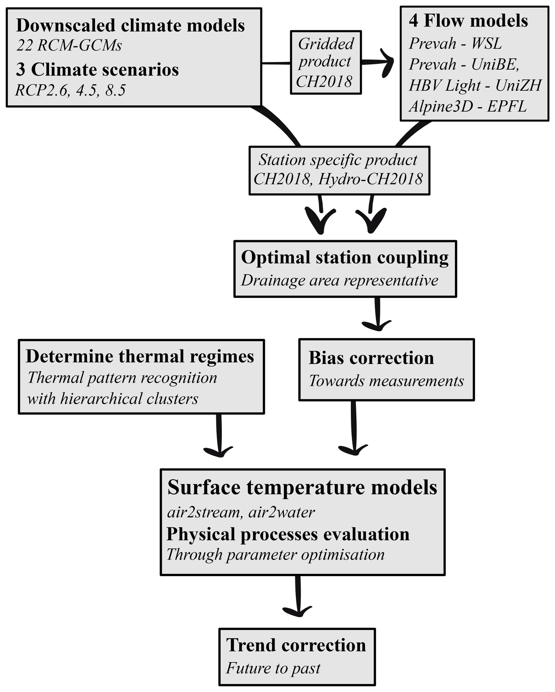
Figure 1 Workflow summarizing the data treatment and the multi-fidelity model selection and optimization.

2.1 Data

River water temperatures are directly influenced by both global and, to an even greater extent, local conditions in and above the drainage area, especially in regions divided by geographic barriers such as mountains (Ficklin et al., 2023). To analyze site-specific controls and to project future river water temperatures, measured historic and simulated future climate data should thus be representative of the conditions and hydrologic processes upstream of the locations to be studied. The air2stream and air2water models require both measured historic and simulated future climate data to extend to at least a year (ideally more than 1) and to be at a daily resolution. However, to be sure that the effect of climate is included in the calibration and analysis of future conditions, data should preferably cover 30 years (WMO, 2017; Piccolroaz et al., 2013).

Temporally overlapping, daily averaged near-surface air temperature and river discharge measurements spanning the 30-year reference period of 1990 to 2020 were used as calibration data, while, for validation, the data from 1980 to 1990 were used (Table S2). By choosing to use the most recent data for calibration rather than validation ensures that recent local climate conditions are carried into future projections (Shen et al., 2022). For the few cases where no forcing data for calibration did exist between 1990 to 2020 (Table S2 in the Supplement), validation was deprioritized, and calibration was performed for the 1980–1990 data.

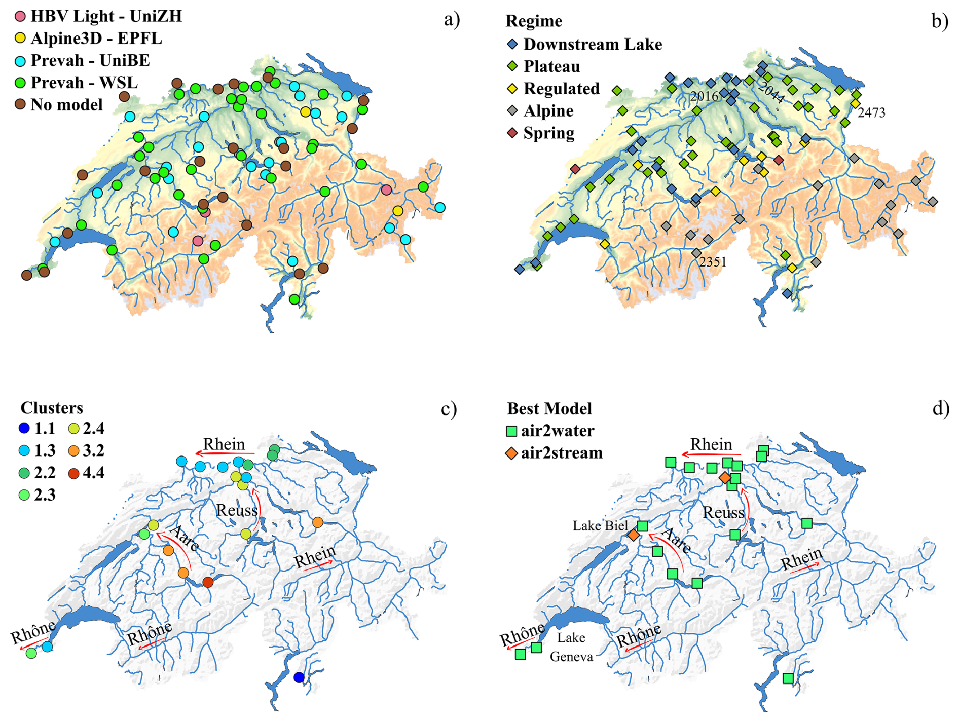
Figure 2 (a) Investigated FOEN stations with available and used hydrological models providing future projections of river flow, (b) station thermal regimes, (c) Downstream Lake clusters, and (d) best-performing surface water temperature model at Downstream Lake stations. Red arrows show river flow directions. The coordinate reference system is the Swiss LV95. The background map is the DHM25, http://www.swisstopo.admin.ch/de/geodata/height/dhm25.html (last access: 1 September 2025).

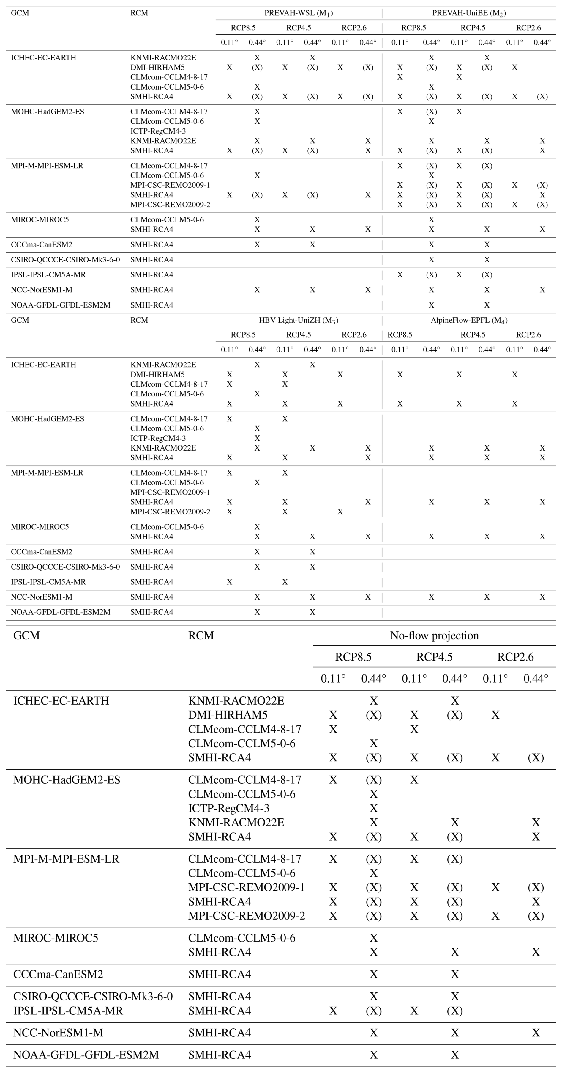
Here, we use CH2018 climate simulations based on the EURO-CORDEX regional climate modeling ensemble. In CH2018, near-surface air temperature was downscaled by applying a statistical bias correction and downscaling method (quantile mapping, a purely statistical and data-driven method) to the original output of all EURO-CORDEX climate model simulations as observational reference station observations and observation-based gridded analyses were used (CH2018, 2018, Chapter 5). These data are available as both gridded and local station products (CH2018 Project Team, 2018). Following CH2018, the Hydro-CH2018 project analyzed the effects of climate change on Swiss waterbodies (FOEN, 2021). The gridded climate product from CH2018 was used to construct projections of future river discharge for four hydrological models used in Hydro-CH2018. The location where output from these four models was used in this study is shown in Fig. 2a, including the following: (M₁) PREVAH-WSL, a conceptual process-based model by Brunner et al. (2019); (M₂) PREVAH-UniBE (Muelchi et al., 2021); (M₃) HBV Light-UniZH, a bucket-type hydrological model (Freudiger et al., 2021); and (M₄) AlpineFlow-EPFL, which is made up of the snowmelt and runoff model Alpine3D coupled to the semi-distributed hydrological model StreamFlow (Michel et al., 2022). The Hydro-CH2018 project produced projections for 61 out of the 82 FOEN river monitoring stations under 22 GCM–RCM model chains (9 GCMs coupled to 8 RCM runs) with 0.11 and 0.44° resolution and three climate change scenarios (RCP2.6, 4.5, and 8.5). The available projections, the employed circulation and hydrological models, and the considered climate change scenarios for all of the different stations that were considered in this study are summarized in Table 1.

Table 1 Climate projections and hydrological models used for temperature simulation. For a complete climate model designation, see the CH2018 project report (CH2018, 2018). Models analyzed are indicated by an “X” mark, and models not analyzed but with simulation data are indicated by a “(X)” mark.

From models M₁–M₃, continuous projections of river discharge at a daily resolution for the entire period covering 1990–2099 were available; projections from the M₄ model were discontinuous and only covered the periods 1990–2000, 2005–2015, 2030–2040, 2055–2065, and 2080–2090. River temperature simulations of river monitoring stations for which forcing data from models M₁–M₃ were available covered the entire period of 1990–2099, while, for stations for which only data from model M₄ were available, simulations were only run for the periods for which data were available.

Measurements of historic meteorologic and hydraulic parameters which were used for model calibration, validation, and bias correction were obtained at a daily resolution from the MeteoSwiss IDAweb platform (http://www.meteoschweiz.admin.ch, last access: 15 December 2024) and from the Hydrology Division of the Federal Office for the Environment (FOEN) (http://www.hydrodaten.admin.ch, last access: 1 September 2025). For monitoring stations at which historic river discharge data or future river discharge projections were not available, only future near-surface air temperature projections were used to simulate water temperature. Where climate projections were available at multiple different spatial resolutions (i.e., 0.11 and 0.44°), only one model, as indicated in Table 1, was included in the analysis, following the approach of Muelchi et al. (2021).

2.2 Hydrologic and meteorologic station coupling

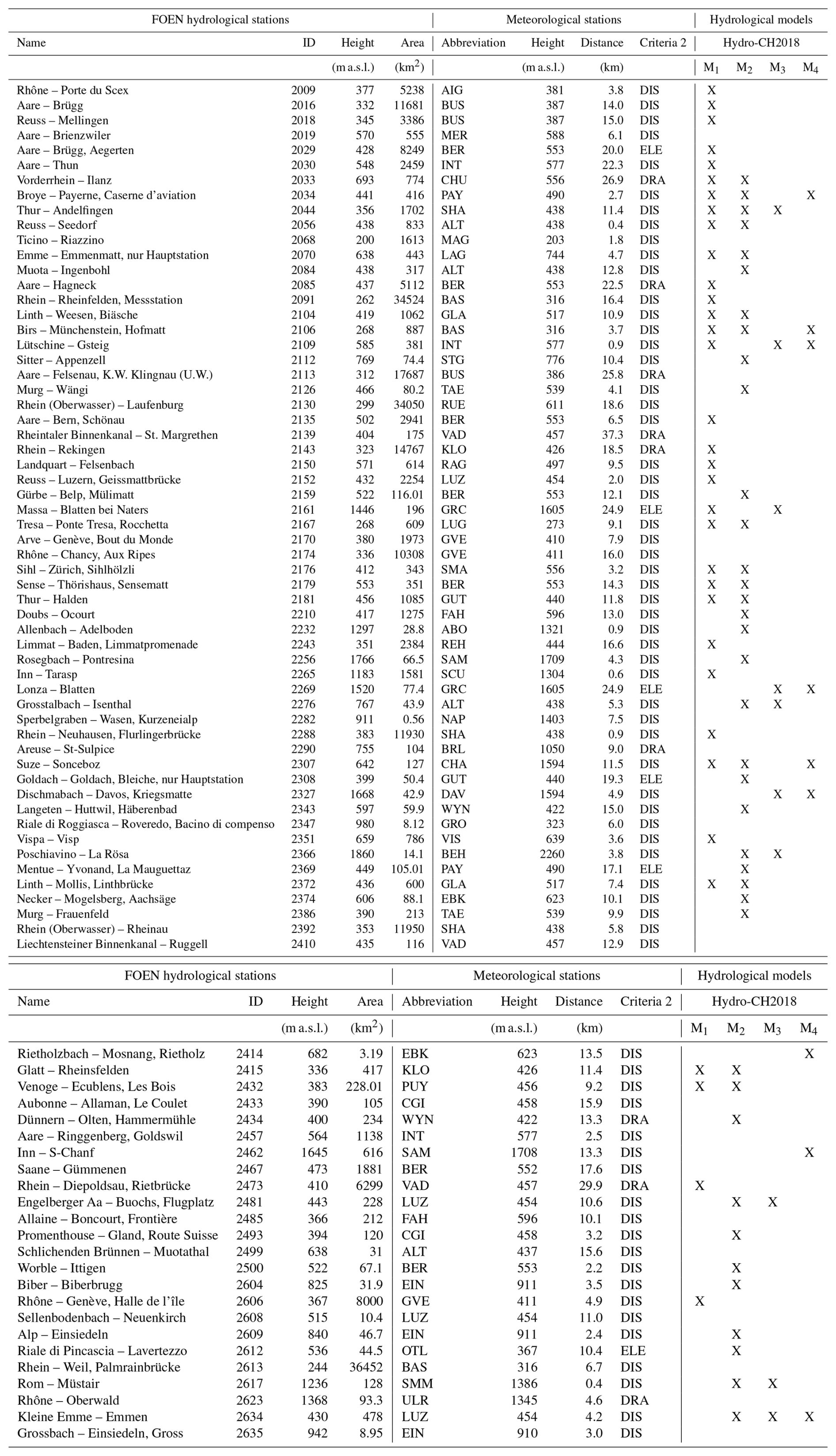
Switzerland is characterized by a pronounced topography. Therefore, the closest meteorological station to a hydraulic station might not necessarily be the ideal coupling partner. Hydrological and meteorological stations were therefore paired according to the following procedure: we only considered stations for which (a) future climate projections of near-surface air temperatures (required) and river discharge (optional but desirable for improved water temperature predictions) were available for the entire period covering 1980 to 2099 and (b) historic measurements of near-surface air temperatures and river discharge were available from 1980 to 2020. Meteorological stations were subsequently paired with hydrological stations such that (a) the horizontal distance between rivers and meteorological stations was as small as possible, i.e., nearest to nearest (criterion: distance or DIS); (b) the meteorological station was representative of the conditions in the upstream drainage area, meaning the meteorological station was located in the same valley and in the upstream region (criterion: drainage area or DRA); and (c) the elevation difference did not exceed a reasonable threshold of 200 m (criterion: elevation or ELE). Where possible, all three criteria were met; that is, the closest station passed both ELE and DRA and is noted as DIS in Table 2. If the closest station was deemed not to be representative (e.g., in a neighboring valley or downstream) and if the DIS criteria were not met, such a station is noted as DRA in Table 2. If a station failed both DIS and DRA but passed ELE, it is noted as ELE in Table 2. Station details and pairings are summarized in Table 2.

Table 2 Combined river and meteorological stations and available models for climate projections of discharge. Abbreviations: DIS – distance, ELE – elevation, and DRA – drainage area.

2.3 Forcing-data bias correction

Differences between near-surface air temperature measurements used for calibration and climate model projections, even when slight, may artificially alter the quantification of projected future river water temperatures by introducing a systematic bias at the start of the simulations. Despite the fact that the highly resolved GCM–RCM output data that were considered were already statistically downscaled, small differences between modeled and observed air temperatures during the reference period could still be detected.

For the river discharge projections, no bias correction has so far been performed. To mitigate this bias, the time series of air temperatures and river discharge used as climate forcing data were statistically adjusted using the change factor method (Diaz-Nieto and Wilby, 2005; Minville et al., 2008). This method first adjusts climate projections in relation to measurements by removing the climatological year (consisting of daily averages) from the modeled data and then adding the corresponding climatological year from measurements according to Eq. (1), thereby correcting long-term and seasonal biases while maintaining individual climate model trends and stochastic variabilities.

$$\begin{array}{}\text{(1)}& {\mathrm{Fn}}_i=\left({\mathrm{Fo}}_i-{\mathrm{Co}}_j\right)+{\mathrm{Cm}}_j\end{array}$$

In the above, Fn_i is the adjusted variable at time i; Fo_i is the simulated future climate time series of either air temperatures or river discharge at a daily resolution; and Co_j and Cm_j are the climatological years of the simulated climate time series and the historic measurements, respectively, on the day of year j corresponding to time i. The climatological years were smoothed using a 60 d window to remove the effect of possible pulse events, especially for discharge. Due to low-flow conditions in some rivers, discharge in the rivers was never adjusted below the minimum observed flow.

2.4 Thermal-regime classification

For the multi-fidelity modeling approach, the different river monitoring stations were re-classified into the four different thermal regimes that have previously been identified for Switzerland (Michel et al., 2020; Piccolroaz et al., 2016), as well as one additional thermal regime defined for the purpose of this study.

The existing thermal regimes are Downstream Lake, Swiss Plateau, Alpine, and Regulated, while the Spring discharge regime was added to address the special thermal case of stations situated at the mouth of spring-fed streams. Downstream Lake stations show a clear decoupling between river temperature and river discharge, Swiss Plateau stations exhibit an annual flow cycle with minimal discharge in summer and strong interannual variability, Alpine stations show that both discharge and temperature are strongly influenced by snow and glacier melt, Regulated stations are fed by intermittent releases of large volumes of water from upstream reservoirs, and Spring stations are located immediately downstream of springs and are characterized by a nearly constant temperature signal decoupled from air temperature.

The already existing classifications from Michel et al. (2020) and Piccolroaz et al. (2016) and the suitability of the yet unclassified stations to be grouped under the different thermal regimes were first explored by evaluating the historic data and the locations visually (Fig. 2b). Following this first visual classification, an automated thermal-pattern recognition using hierarchical clusters via the cluster tool DTWARP_PER_33 (Bögli, 2020) was used (Fig. 2c). Application of the thermal-pattern recognition matched the visual pre-classification in most cases but revealed that, for certain stations located far downstream of lakes, upstream lake processes are still the dominant control for river water temperatures. Stations that were previously classified as not being part of the Downstream Lake regime were thus reclassified here as Downstream Lake according to the results of the thermal-pattern recognition procedure.

2.5 Surface water temperature model setup

Two semi-empirical surface water temperature models were employed: the river water model air2stream (Toffolon and Piccolroaz, 2015; http://www.github.com/marcotoffolon/air2stream, Toffolon and Piccolroaz, 2016b), whereby we use version 2 of air2stream (Piccolroaz et al., 2016, https://github.com/spiccolroaz/air2stream, Piccolroaz 2016b), and the lake water model air2water (Piccolroaz et al., 2013; http://www.github.com/marcotoffolon/air2water, Toffolon and Piccolroaz, 2016a), with air2stream being an extended version of air2water. Both the air2stream and the air2water models combine the simplicity of stochastic models with accurate empirical representation of the relevant physical processes affecting water temperature. The models require near-surface air temperature as input to predict future river temperature, while discharge may optionally be incorporated into air2stream to further improve river temperature predictions.

Both models include up to eight parameters (a₁ to a₈) which are fitted to measured data. Apart from the effect of air temperature on water temperature, the models also resolve the effect of river depth, discharge, thermal signals from tributaries, inverse stratification in lakes during winter, and seasonal cycles. Model complexity, i.e., how many processes are directly resolved by the models or indirectly included through parameter estimation, can be varied by removal of one or more of the additional processes listed above, resulting in the use of eight, seven, six, five, four or three parameters. Depending on local conditions, model performance can be improved by the removal of processes which play a minor or insignificant role in relation to water temperature. Where this simplification with the removal of parameters was done (Table S2), removed processes plays a minor role in the simulation of water temperature, as evident in the decreased model performance while being included. For additional information about air2stream and air2water see Supplement Sect. S1 and Piccolroaz et al. (2013) and Toffolon and Piccolroaz (2015).

For the simulation of future river temperatures, a multi-fidelity modeling approach that identified the best water temperature model for each single river monitoring station was employed. The optimal model parameter configuration for each station was identified via a Monte Carlo calibration process performed with the Crank–Nicolson scheme (Crank and Nicolson, 1947), consisting of over 2000 runs using particle swarm optimization (Kennedy and Eberhart, 1995) with 500 particles. The root mean square error (RMSE) function was used as the objective function and combined with the dotty-plot quality check (Piccolroaz et al., 2013; Piccolroaz, 2016a; Toffolon et al., 2014).

For stations missing either historical data or future projections of river discharge (brown markers, Fig. 2a), discharge was not considered as forcing data, and the air2stream model was reduced to a three- or five-parameter model, while no adaptation was required for the air2water model as it does not simulate discharge. Datasets used for calibration and validation with data gaps shorter than 30 d were filled by linear interpolation, while, for datasets with gaps exceeding 30 d, only the longest continuous dataset was used.

All simulations (calibration, validation, and climate runs) used a 1-year period as a spin-up, with the first year of forcing data repeated. Only the best-performing river temperature model was considered for the follow-on climate runs. The final calibration and validation periods and the best-performing parameter setups for each station are provided in Table S2 (Sect. S2). As initial conditions for the stepwise climate simulations with model M₄, we used simulated temperatures from the latest prior simulated date; that is, for simulations between 2030 to 2040, we used temperature from the end of 2015 as the initial condition.

At Downstream Lake stations, multiple configurations of both water temperature models (air2stream and air2water) were tested through calibration, and only the best-performing temperature model and parameter setup were kept (station thermal regimes, as well as cluster results, are shown in Fig. 2 and provided in Table S1 in Sect. S2 of the Supplement). For the remaining stations not belonging to the Downstream Lake regime, river processes such as local flow variations and water depth dominate the water temperature development. For these stations, different model configurations of only the air2stream model were explored.

2.6 Trend correction

Empirical models generally predict less warming in the future compared to physically based models, with the primary reason for this being underrepresentation of the thermal catchment memory, including snow and ice (Leach and Moore, 2019). To quantify how well the models air2stream and air2water, which both lack deterministic considerations of snowmelt and ice melt, are able to recreate past trends, we compared trends from river water temperature measurements and corresponding modeled temperature trends between 1990 and 2019. On an annual basis, this comparison was possible for 25 out of 82 river stations, consisting of 9 Downstream Lake, 7 Regulated, 7 Swiss Plateau, 2 Alpine, and 0 Spring thermal-regime river stations. Stations were selected with a requirement of 30 years of continuous data on air and water temperature and river discharge. Only statistically significant trends (p<0.05) were considered.

On average, both air2stream and air2water underestimate the annual temperature trend during the reference period by 0.14 and 0.11 °C per decade, respectively. For air2stream, the annual trend bias is smallest for the Swiss Plateau thermal regime (0.09 °C per decade) and largest in the Alpine thermal regime (0.17 °C per decade). Seasonally, the trend bias is largest from June to August and September to November, whereas, especially for air2water, the bias is small from December to February and March to May.

The divergence of both the air2stream and air2water models from observed trends warrants a post-simulation bias correction of simulated trends. The bias is river station dependent, making an individual correction at each station preferable (Tables S3 to S6 in Sect. S2). However, only about 30 % of the river stations investigated have long enough datasets (30 years) for individual correction. Therefore, we tied the seasonal trend bias correction to the thermal regime, thereby keeping the correction linked to local conditions. Note that no river station of the Spring thermal regime had enough data to allow for the trend bias correction. Spring river stations were therefore not trend bias corrected. As the trend bias correction acts on climate simulations of river temperature stretching from 1990 to 2099, the bias correction had to be scaled in relation to how air temperature trends shift in the climate models. The scaling was designed such that it did not affect the bias correction during the reference period (1990 to 2019) while adjusting the correction in relation to how the air temperature trend (TTair) changes in the near-future (2030 to 2059) and far-future (2070 to 2099). For this purpose, an adjustment factor Fs (–) was constructed from the mean climate model air temperature trends for each climate scenario. Fs is thus specific for each climate scenario, river station, and season.

$$\begin{array}{}\text{(2)}& {\mathrm{Fs}}_{i,\mathrm{s}}={\displaystyle \frac{{\mathrm{TTair}}_{i,\mathrm{s}}}{{\mathrm{TTair}}_{\mathrm{ref},\mathrm{s}}}}\end{array}$$

Here, TTair_i,s is the mean of the air temperature trends from the climate models, which changes for each season and with the reference, near-future, and far-future periods; TTair_ref,s is the mean of the seasonal air temperature trend during the reference period; i is the number of days; and s denotes the season. The temporal gaps between 1990 to 2019, 2030 to 2059, and 2070 to 2099, during which the air temperature trends were calculated, were linearly filled with shape-preserving piecewise cubic interpolation resulting in a continuous factor Fs_i,s from 1990 to 2099. Fs_i,s varied from −2 to +3 depending on the season and climate scenario and was applied for simulations using discharge input from models M₁ to M₃, while, for simulations using M₄, Fs_i,s was set to 1 from 1990 to 2099 due to too-short simulation time frames in M₄ (only 1 decade). With Fs_i,s, the seasonal and thermal-regime-dependent water temperature bias Tb_i,s (regime-dependent mean from Tables S3 to S6 in Sect. S2) is turned into the thermal-regime- and climate-scenario-dependent seasonal bias correction Bc_s (°C d⁻¹):

$$\begin{array}{}\text{(3)}& {\mathrm{Bc}}_{\mathrm{s}}=\sum _{i=\mathrm{1}}^{i=n}{\mathrm{Fs}}_{i,\mathrm{s}}\cdot {\mathrm{Tb}}_{i,\mathrm{s}},\end{array}$$

where n is the number of days since 1 January 1990. Before adjusting the water temperature model output from 1990 to 2099, the seasonal Bc_s was combined into a continuous dataset Bc. To avoid a sharp shift in Bc between each season, a 3 to 5 d gap in between each season was smoothed with shape-preserving interpolation (piecewise cubic Hermite interpolation, PCHIP; MATLAB R2022a).

The trend adjustment applied here with Fs, Bc, and pre- and post-adjustment data is shown for one example station in Fig. S1 in the Supplement (Sect. S2). Pre- and post-trend correction for the difference in modeled and measured trends is summarized in Table S7 (Sect. S2).

2.7 Thermal hysteresis

Hysteresis, wherein a dependent variable (water temperature or suspended sediments) can exhibit multiple values in response to a single value from the independent variable (discharge), is a common phenomenon in hydrology (Gharari and Razavi, 2018). Sediment transport hysteresis can be caused in rivers by emptying and refilling sediment layers on the riverbed (Tananaev, 2012) and through erosion on land, as shown in the Alps, with the contributing location (riverbed or eroded area) determining the hysteresis loop shape and rotation direction (Misset et al., 2019). Stream temperature can also show hysteresis effects, with the example being a lag in the response to air temperature caused by ice melt or reservoir release (Van Vliet et al., 2011; Webb and Nobilis, 1994).

We investigated past and future hysteresis loops between water temperatures (the dependent variable) and river discharge (the independent variable) using a versatile index (the Zuecco index, Zuecco et al., 2016). The Zuecco index works through the computation of definite integrals based on data in chosen intervals and was developed for hysteretic loops where the independent variable increases from its initial value, reaches a peak, and then decreases. The index divides loops into classes depending on rotation direction (counterclockwise or clockwise), number of loops, and loop sizes.

Here, we use Zuecco classes I to IV (Fig. 3, left column), which represent the interaction between flow and water temperature for the cases of datasets starting with low temperature and low flow. However, mainly in the Swiss lowland at the beginning of a year, rivers can display a situation where the temperature is cold (low) and flow is high, followed by a higher temperature in spring combined with less water. This process has been shown to be enhanced by the ongoing climate warming through the shortening or elimination of snow cover and glacial melt (FOEN, 2021; Michel et al., 2020; Van Vliet et al., 2013).

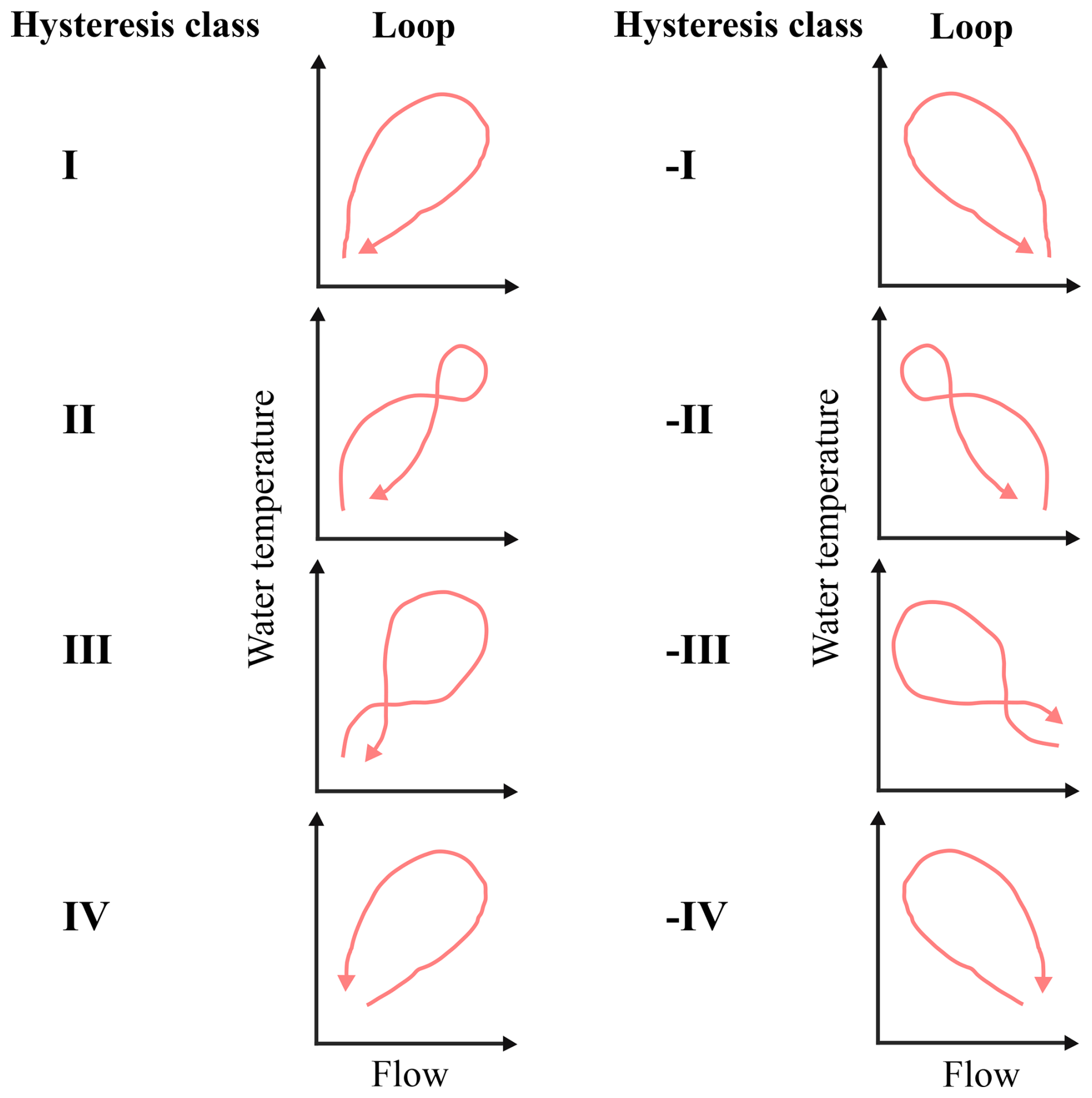
Figure 3 Hysteresis classes with corresponding hysteresis loops. Expanded with classes -I to -IV from Zuecco et al. (2016) to incorporate water temperature as the dependent variable.

To incorporate this reversed hysteretic loop, we added four mirrored hysteresis classes, -I to -IV, to the classes introduced by Zuecco et al., (2016) (Fig. 3, right column). This was done by inverting the normalized flow prior to the computation of definite integrals, thus creating an increasing and decreasing independent variable. Note that the index works on set intervals. If the loops do not come back to their initial values, it works with open loops. The length of the datasets being investigated should depend on the quality and resolution of the data and the rate at which the dependent variable changes with respect to the independent variable (Zuecco et al., 2016). Here, we used daily resolved datasets, averaged from 30 years of modeled data and, thus, always providing full annual loops.

2.8 Temperature extremes

Extreme conditions depend on what is considered to be extreme in relation to normal conditions (Stephenson, 2008). Here, water temperatures are considered to be extremely high if they exceed the 90th percentile during the 30-year reference, near-future, and far-future periods (IPCC, 2014).

We define a new extreme-event severity index as the temperature difference between the 90th percentile and the median for each climate simulation and period. If this temperature gap increases, it indicates that extreme temperatures become more severe as thermal peaks are elevated compared to the median temperature. The extreme-event severity index for each simulation and period is thus X °C from 0 °C, where X denotes the difference between the 90th percentile and the median temperature, while 0 °C represents a match to the median temperature. Our analysis was made to be independent of when (beginning or end) in the 30-year periods it was conducted by removing the climatic trend for each simulation and period before calculating the index. Note that, by defining extreme events with the 90th percentile during each analyzed period, we consider temporal in situ extreme events as they are experienced during the considered periods. We do not inflate our results by using past extreme event definitions to evaluate future extreme events.

2.9 Thermal thresholds for fish

By counting the number of days per year during which thermal thresholds are exceeded, effects of climate change on fish can be evaluated both locally and regionally (Michel et al., 2020). The occurrence of exceedance of specific river water temperature thresholds on a daily scale was used to investigate the historic past (1990 to 2019) and projected future (2070 to 2099) stress on the brown trout (Salmo trutta). Three thermal thresholds were chosen in order to incorporate important aspects in the life of the brown trout, including (1) adult mortality as a result of a daily mean temperature above 25 °C (Elliott, 1981; Wehrly et al., 2007), also set as a hard upper limit for the thermal use of waters in Switzerland (Water Protection Ordinance 814.201); (2) an increased risk for parasite-caused proliferative kidney disease (PKD) as a result of a daily mean temperature above 15 °C (Chilmonczyk et al., 2002; Strepparava et al., 2018); and (3) fish egg (roe) mortality from September to January as a result of a daily mean temperature above 13 °C (Elliott, 1981).

3 Results

3.1 Warming

The most influential factor for future river water temperatures is the climate change scenarios. Individual river water warming for the different stations, from the reference (1990–2019) to the near-future (2030–2059) and far-future (2070–2099) periods, is shown in Fig. 4. Under the RCP8.5 scenario, the warming of river temperatures increases throughout the 21st century and even accelerates. The smallest change in river temperatures was observed under the RCP2.6 scenario, with warming reaching a plateau in the middle of the 21st century. The mean change in river temperatures from the reference period to the near-future and far-future amounts to +0.77 and +0.91 °C for RCP2.6, +0.95 and +1.51 °C for RCP4.5, and to +1.22 and +3.18 °C for RCP8.5, respectively. This amounts to an averaged water warming rate from 1990 to 2099 for RCP8.5 of 0.36 °C per decade, 0.19 °C per decade for RCP4.5, and 0.12 °C per decade for RCP2.6. At the same time, near-surface air temperature changed by 0.50 °C per decade for RCP8.5, 0.26 °C per decade for RCP4.5, and 0.13 °C per decade for RCP2.6.

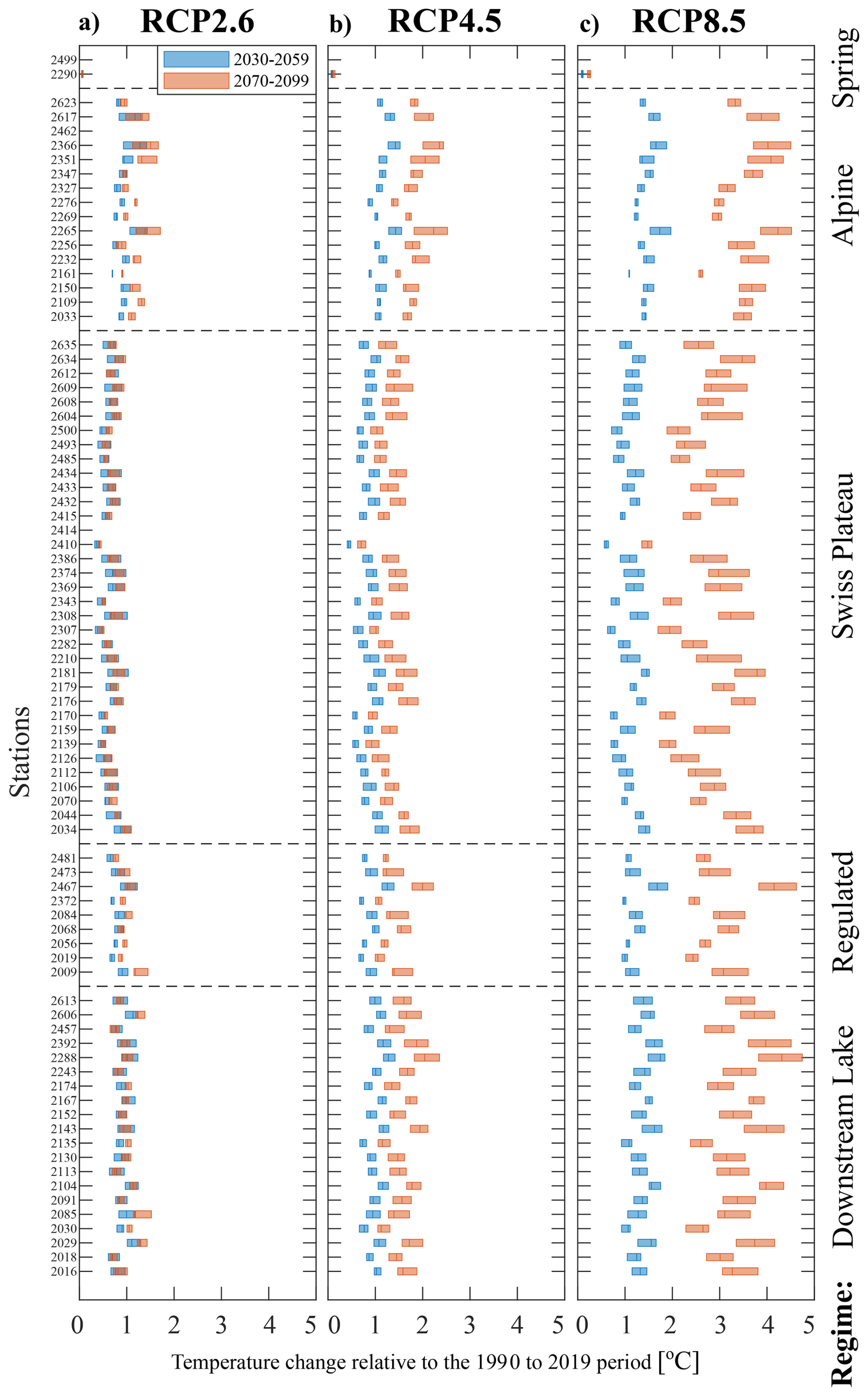
Figure 4 Modeled mean river temperature increase from the reference (1990 to 2019) to the near-future (2030 to 2059, blue bars) and far-future (2070 to 2099, red bars) under climate scenarios RCP2.6, RCP4.5, and RCP8.5. Shown is the median (bar center line) and the lower and upper quartiles (left and right bar extent) of the difference between periodic mean temperatures (over 30 years) for each available climate simulation, additionally averaged where multiple hydrological models exist (M₁, M₂, M₃); i.e., the bar extents show climate model variability in the mean temperature change between the three periods. Station nos. 2414 and 2462 are not shown since the flow model M₄ lacked 30 years of continuous data.

Climate change impact was heterogeneous between stations, yet common patterns were found within thermal regimes (Fig. 4, Table S8 in Sect. S2). The strongest river water warming, regardless of climate scenario or time period, was observed for stations in the Alpine thermal regime, followed, in order, by Downstream Lake, Regulated, Swiss Plateau, and Spring thermal regimes. Under RCP8.5, on average, the river temperatures of Alpine stations warm by 1.44 °C until the near-future and by 3.54 °C until the far-future compared to the reference period. The river water of Downstream Lake stations also warmed strongly by 1.36 °C until the near-future and by 3.43 °C until the far-future. Compared to the Alpine and Downstream Lake thermal regimes, river temperatures of stations in the Regulated (near-future: +1.19 °C; far-future: +3.00 °C) and Swiss Plateau (near-future: +1.06 °C; far-future: +2.75 °C) thermal regimes warmed less. Least affected, by a wide margin, were the river temperatures of the two stations that can be classified as being in the Spring thermal regime (near-future: +0.04 °C; far-future: +0.10 °C).

3.2 Hysteresis analysis

The hysteresis class could be determined for each station with future and present river discharge (47 out of 82 stations). For all stations, climate scenarios, and climate models, the index found solutions in hysteresis intervals ranging from 164 to 328 d. During the reference period, the dominant hysteresis class was IV (45.6 %), followed by III (25.0 %), -I (14.7 %), -II (11.8 %), and I (2.9 %), while no stations belonged to class II. For the reference period, the classes remained independent in relation to the climate scenario (RCP8.5, 4.5, 2.6) or hydrological model (M₁, M₂, M₃) used, while, in the near-future and far-future, differences start to show. For RCP8.5, in the far-future period, the dominant class was -I (48.5 %), followed by class IV (33.8 %), III (13.2 %), and -II (4.4 %).

For the RCP8.5 scenario, classes are shown for the reference, near-future, and far-future periods in Table 3 (hysteresis classes for RCP4.5 are shown in Table S9, and hysteresis classes for RCP2.6 are shown in Table S10; both are shown in Sect. S2). Under RCP8.5, the number of stations which changed hysteresis classes between the reference and the near-future was 23 %, increasing to 51 % for the far-future. Correspondingly, under RCP4.5, 23 % changed hysteresis classes when reaching the near-future, while 38 % of the stations changed classes when reaching the far-future. Under RCP2.6, 28 % of stations changed classes when reaching the near-future, but once reaching the far-future, some stations changed back again, and the fraction of stations that were in a different hysteresis class compared to the reference period was reduced to 21 %.

Table 3 Modeled hysteresis classes during the reference (1990 to 2019), the near-future (2030 to 2059), and the far-future (2070 to 2099) periods for climate scenario RCP8.5. Flow data are from models M₁, M₂, and M₃. Stations that had no flow measurements for calibration, that were missing flow model output as forcing, or where the use of the air2water model did not require flow as input have been excluded. A change in class from the reference period to the near- or far-future period is highlighted in italics. Classes are shown as natural numbers instead of Roman numerals for ease of reading.

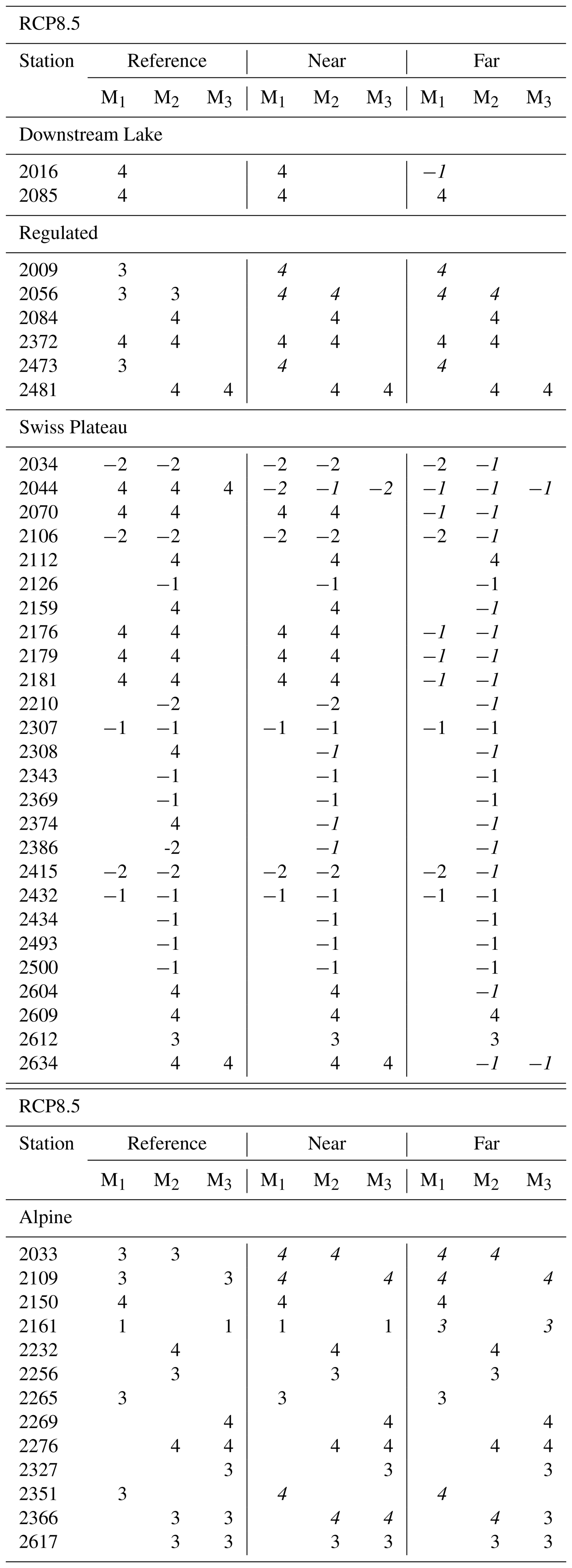
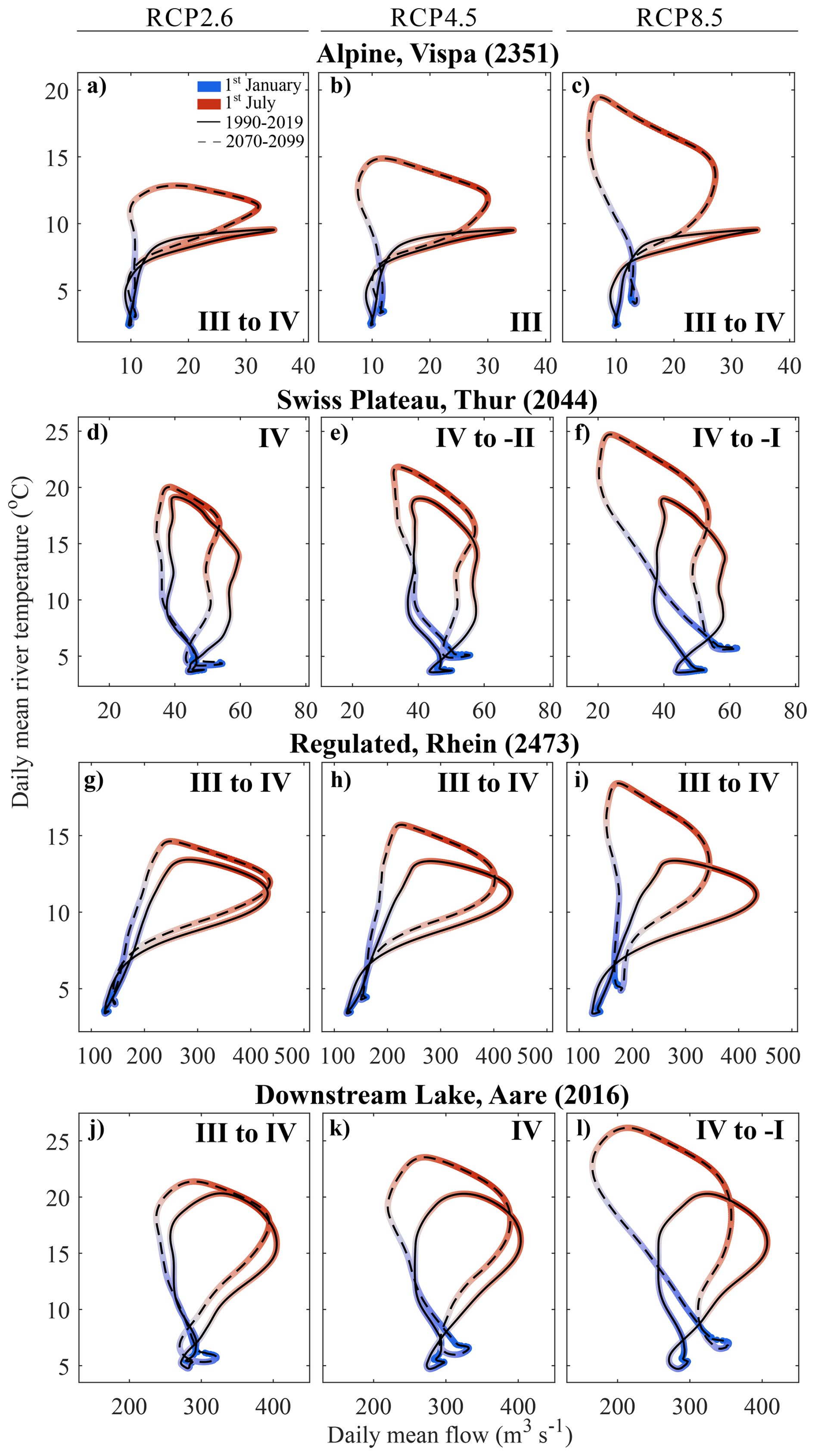
Figure 5 Daily averaged river discharge and water temperature for the reference (1990 to 2019, solid line) and the far-future period (2070 to 2099, dashed line) at four stations showing the current and the future thermal hysteresis loops. Flow data used are from model M₁; stations belong to the Alpine, Swiss Plateau, Regulated, and Downstream Lake thermal regimes. Daily averaged datasets have been smoothed twice with a running average of 30 d. Hysteresis class change is shown in roman numerals (see Fig. 3); station locations are shown in Fig. 2b.

Considering only the far-future period (2070 to 2099), stations belonging to the Swiss Plateau thermal regime showed the largest change in hysteresis loop classes, with 58 % changing under RCP8.5, 42 % changing under RCP4.5, and 12 % changing under RCP2.6. Considering again only the far-future, stations belonging to the Regulated thermal regime exhibited hysteresis loop class changes of 50 % under RCP8.5, 33 % exhibited changes under RCP4.5, and 50 % exhibited changes under RCP2.6. Least prone to hysteresis class changes in the far-future were stations of the Alpine thermal regime (38 % under RCP8.5 and RCP4.5, 23 % under RCP2.6). Out of the 20 Downstream Lake thermal-regime stations, only 2 stations were investigated with discharge (i.e., modeled with air2stream instead of air2water). From these two stations, one changed hysteresis class under RCP8.5 by the far-future, one changed under RCP2.6, but none changed under RCP4.5. As can be seen from the four representative stations for the Swiss Plateau, Regulated, Alpine, and Downstream Lake regimes, as illustrated in Fig. 5, a change in hysteresis class is usually associated with a counterclockwise rotation and stretching of the loop from, for example, a lower to a higher class (III to IV). Such rotation and stretching appear to be a result of increased warming in summer combined with a decrease in summer discharge, while warming is smaller and discharge is increased in winter compared to in summer.

3.3 Temperature extremes

The analysis is focused on temperature extremes in the summer months (June to August), during which the severity of extremes varies in between climate scenarios and is different on an individual-station basis and on a thermal-regime basis (Fig. 6). Note that the use of extreme-event severity as an index should be viewed as the minimum temperature increase of extreme events in the future, while it denotes the increase in the 90th percentile. From the reference (1990 to 2019) to the far-future (2070 to 2099) period, the extreme-event severity for scenario RCP2.6 increased, on average, by +0.20 °C (Fig. 6a), by +0.38 °C for RCP4.5 (Fig. 6b), and by +0.61 °C for RCP8.5 (Fig. 6c).

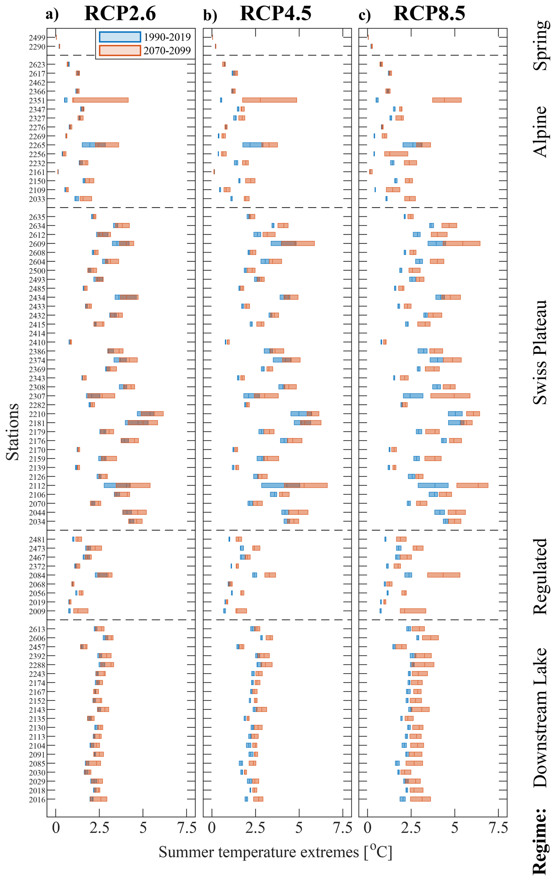
Figure 6 Severity of water temperature extremes from June to August for 30 years of climate simulations (blue bars: 1990 to 2019; red bars: 2070 to 2099) ordered according to thermal regime. Shown are the lower and upper quartiles (extent of bar) and the median (bar center line) of the difference between the 90th percentile and the seasonal median temperature (30 years of data) from all available climate models, additionally averaged where multiple hydrological models exist (M₁, M₂, M₃) at each station and time period; i.e., the bar extents show climate-model-induced variability in each period. Station nos. 2414 and 2462 are not shown since the flow model M₄ lacked 30 years of continuous data.

Looking at extreme events at the level of thermal regimes, during the reference period (1990 to 2019), the most severe extreme temperatures occurred at stations in the Swiss Plateau and Downstream Lake thermal regimes. The Swiss Plateau thermal regime showed a mean extreme-event severity of +2.8 °C, that of the Downstream Lake thermal regime was +2.2 °C, that of the Regulated regime was +1.3 °C, that of the Alpine regime was +1.1 °C, and that of the Spring thermal regime was +0.12 °C.

For all climate scenarios and all thermal regimes, the severity of extreme events increased throughout the 21st century. For the far-future (2070 to 2099), under all climate scenarios, the Swiss Plateau and the Downstream Lake thermal-regime stations remain the stations with the severest extreme events, while the extreme-event severity increases the most for the Regulated and the Swiss Plateau thermal regimes. As the Swiss Plateau and Regulated thermal-regime stations are mostly located in the Swiss lowland in the northwestern part of Switzerland (see Fig. 2b), they are the ones that are expected to experience the most severe low-flow conditions, especially in summer months under the RCP8.5 scenario, with a discharge reduction ranging from 5 % to 60 % (FOEN, 2021; Brunner et al., 2019; CH2018, 2018). The largest increase from the reference to the far-future period was found at stations for the Regulated thermal regime (mean extreme-event severity increase under RCP2.6: +0.28 °C; under RCP4.5: +0.54 °C; under RCP8.5: +0.93 °C) followed by the Swiss Plateau (RCP2.6: +0.26 °C; RCP4.5: +0.48 °C; RCP8.5: +0.78 °C), Alpine (RCP2.6: +0.23 °C; RCP4.5: +0.45 °C; RCP8.5: +0.68 °C), Downstream Lake (RCP2.6: +0.23 °C; RCP4.5: +0.40 °C; RCP8.5: +0.61 °C), and Spring thermal regimes (RCP2.6: +0.01 °C; RCP4.5: +0.01 °C; RCP8.5: +0.03 °C).

3.4 Thermal thresholds

Our results show clear thermal-regime-dependent differences for the present and future thermal-related stress on the brown trout (Fig. 7). The lethal threshold (25 °C) was seldom exceeded in the past (Fig. 7a). However, towards the end of the 21st century, for a majority of stations in the Downstream Lake and Swiss Plateau thermal regimes, the lethal threshold was exceeded on at least 1 d during the year, making areas which could previously be considered to be safe for the brown trout potentially lethal, at least on certain days of the year. In addition, the 25 °C limit is also critical for anthropogenic water use in Switzerland as the Swiss law (Water Protection Ordinance 814.201) prohibits a thermal use of waters for cooling purposes beyond this threshold. Unfortunately, our results show not only an increased occurrence of lethal temperatures but also that the less imminently lethal but nevertheless detrimental lower temperature threshold of the increased occurrence of the PKD disease (15 °C) will be exceeded much more frequently (see Fig. 7b), as will the threshold for fish egg mortality (Fig. 7c). Alpine and, to a lesser extent, Regulated thermal-regime stations, where, previously, the thermal conditions for an increased likelihood of PKD were not met, are also likely to exhibit these conditions in the warmer summer months. Given the 153 d from September to January, egg development (approx. 30 to 90 d; Alp et al., 2010) should still have enough time to take place safely throughout the 21st century in Regulated, Swiss Plateau, Alpine, and Spring thermal-regime rivers. Rivers in the Downstream Lake thermal regime are likely to be too large to facilitate spawning and were therefore not considered further in this analysis.

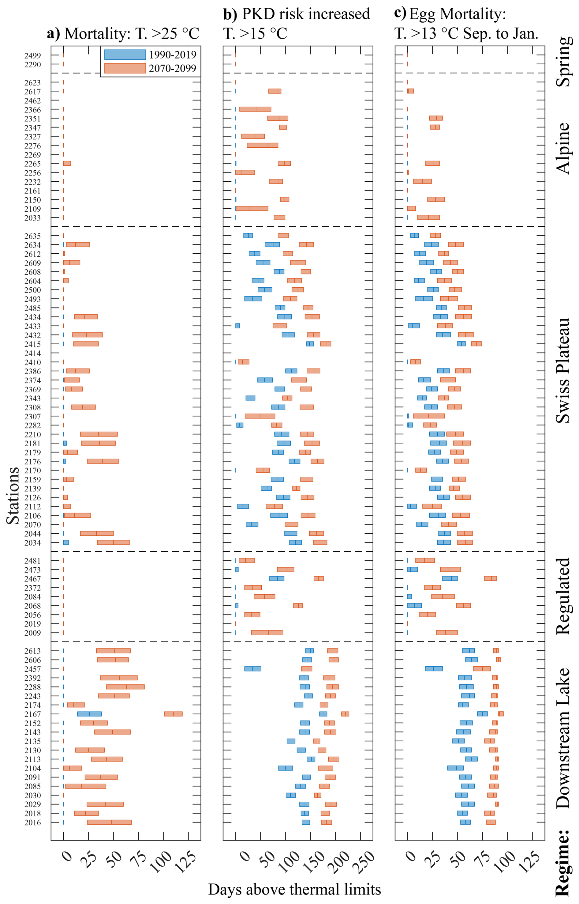
Figure 7 Number of days superseding the thermal threshold for the brown trout for the RCP8.5 climate scenario. (a) Mortality threshold at daily mean temperatures > 25 °C, (b) increased risk for proliferative kidney disease (PKD) at daily mean temperatures > 15 °C, and (c) egg mortality during September to January at temperatures > 13 °C. Data consist of 30 years of climate simulations (blue bars: 1990 to 2019; red bars: 2070 to 2099) ordered according to thermal regime. Shown are the median (bar center line) and the lower and upper quartiles (left and right bar extent) of the climate simulation from all available climate models, additionally averaged where multiple hydrological models exist (M₁, M₂, M₃); i.e., the bar extents show climate-model-induced variability for each period with an annual resolution. Station nos. 2414 and 2462 are not shown since the flow model M₄ lacked 30 years of continuous data.

The results presented below represent the number of stations where the daily temperature was above a given thermal threshold (bar center line above 0 in Fig. 7). Under the RCP8.5 scenario, from the reference to the far-future periods, the number of stations exceeding the mortality threshold (25 °C) increased from 4 to 37 stations out of a total of 54 stations in the Downstream Lake and Swiss Plateau thermal regimes (Fig. 7a). For the Regulated, Alpine, and Spring thermal-regime stations, none passed the lethal threshold during the reference period, but for the far-future, 1 out of 26 stations exceeded it. For Downstream Lake and Swiss Plateau thermal-regime stations, the PKD threshold (15 °C) was largely exceeded during the reference period already (52 of 54 stations), increasing to all stations in the far-future (Fig. 7b). For the Regulated, Alpine, and Spring thermal-regime stations, 2 out of 26 stations exceeded the PKD threshold during the reference period already. While, in the far-future, 20 out of 26 Regulated, Alpine, and Spring thermal-regime stations broke through the 15 °C threshold. With respect to fish egg mortality (13 °C) from September to January, all Downstream Lake thermal-regime stations exceeded this threshold in both the reference period and the far-future period (Fig. 7c). During the reference period, 4 out of 9 Regulated and 31 out of 34 Swiss Plateau thermal-regime stations exceeded the 13 °C threshold. Correspondingly, for the Regulated and Swiss Plateau thermal regimes, 8 out of 9 and all 34 stations, respectively, exceeded the 13 °C threshold during the far-future period. Although Alpine thermal-regime stations never exceeded the 13 °C threshold during the reference period, 8 out of 16 stations exceeded this limit during the far-future period. From the two groundwater-fed spring stations, the mortality, the PKD, and the fish egg mortality thresholds were not exceeded.

4 Discussion

4.1 Multi-fidelity modeling approach

The use of semi-empirical models, by definition, means that some of the physical processes affecting heating are simplified under parametrization and some are directly resolved. The models air2stream and air2water resolve the effect of river depth, discharge, thermal signals from tributaries, inverse stratification in lakes during winter, and seasonal cycles. The heat flux between the atmosphere and surface waters (latent and sensible heat, shortwave and longwave radiation) is not directly resolved by air2stram and air2water. However, indirectly, we consider climate-related heat budget changes in our method through the use of high-quality projections of air temperature and discharge as model input. Glacier retreat is included in the hydrological models providing discharge projections to this study (e.g., Muelchi et al., 2021); however, for temperature, this effect is only indirectly considered in air2stream in relation to reduced water availability in summer. The cooling effect on river water caused by meltwater from snow and ice does not change in our method; as snow and ice recede in a future climate, it is expected that warming in high-altitude rivers is larger than projected in this study. Therefore, if the relationships between discharge and air temperature in relation to water temperature remain similar in the future, our method can be used to reliably project future river temperatures. Importantly, the lower-fidelity water temperature model approach used here, combined with high-fidelity climate and/or hydrological model outputs as input, enables the principles of multi-model ensembles, comparison, and analysis that are required for robust climate change impact assessments (Duan et al., 2019).

To expand on previous results of river water temperature projections for Switzerland (Michel et al., 2022), we employed a multi-fidelity modeling approach that is able to automate the generation of water temperature simulators for the different national river temperature monitoring stations of Switzerland, as summarized in Fig. 1. Models of varying complexity were built by integrating high-fidelity climate and hydrological modeling outputs (i.e., downscaled climate (Table 1) and hydrological model outputs (Fig. 2a) – CH2018 and Hydro-CH2018) with low-fidelity river temperature models of varying degrees of parametrization, i.e., air2water and air2stream (Toffolon and Piccolroaz, 2015; Piccolroaz et al., 2013). Statistical learning-based coupling of atmospheric and hydrological stations (Table 2) and classification of river stations into thermal regimes (Fig. 2b and c) enabled optimal low-fidelity model selection (Fig. 2d) and parametrization.

4.2 Adjustment of trends

A trend bias correction was applied to the temperature model outputs due to the difference observed between modeled and measured trends (Tables S3 to S6 in Sect. S2). The correction decreased the difference between modeled and measured annual trends by approximately 0.1 °C per decade. After the bias correction, modeled annual trends with climate simulations as inputs followed the observed trends closely (Table S7 in Sect. S2). Pre-adjustment climate scenarios have a different bias compared to measurements, with RCP8.5 simulations following the observed trends most closely, while RCP2.6 simulations exhibit the largest bias. This discrepancy in bias is caused by the averaging of trends from up to 22 (RCP8.5), 17 (RCP4.5), or 9 (RCP2.6) climate simulations. The trend bias adjustment was applied seasonally, resulting in an adjustment of 0.12 °C per decade on average. The largest adjustment was required for the period of June to August (0.22 °C per decade), while the smallest adjustment was made for the period of December to February (0.05 °C per decade). Note that only 2 out of 16 Alpine stations had long-enough measured datasets (i.e., 30 years) to derive a historical trend, and that trend was used to adjust all 16 stations. The trend adjustment upscaled from 2 to 16 Alpine stations, as well as the calibration at these stations, could thus benefit from longer time series; we therefore recommend care while using these bias-corrected data. Additionally, for the groundwater-fed station (no. 2499) in the Spring thermal regime, measured water temperature is inversely correlated to air temperature. The result is a near-zero or negative trend for the future (below 0 in Fig. 4). Although the modeled trend at station no. 2499 is statistically significant, the result indicates a limitation in the air2stream model with regard to effectively resolving groundwater-dominated processes under climate change.

4.3 Warming rates, trends, and hysteresis analysis

As expected, the climate scenario turned out to be the most important factor for river water temperature increases, with RCP8.5 being the scenario with the largest warming rate, resulting in an average river water temperature increase of +3.2 °C (+0.36 °C per decade from 1990–2020 to 2070–2099) compared to warmer air temperatures of +0.49 °C per decade. This is in agreement with previous findings for Swiss rivers, which projected a water temperature increase of up to +3.5 °C from 1990–2000 to 2080–2090 or +0.38°C per decade (Michel et al., 2022) compared to a measured water temperature increase of +0.33 °C per decade from 1979 to 2018 (Michel et al., 2020), as well as for Swiss lake surface water temperatures, which were projected to increase by +3.3 °C from 1982–2010 to 2071–2099 (Råman Vinnå et al., 2021). In addition to the strong warming of water temperatures until the end of the century, the projections made herein also suggest that the seasonal patterns in the warming of near-surface air temperatures in Switzerland are going to persist in river water temperatures, with stronger warming in summer compared to winter.

Among the different stations, common patterns and trends in river temperature warming could be identified by classifying the stations into the four different river thermal regimes occurring in Switzerland (Piccolroaz et al., 2016). The classification was further improved in this study by adding a groundwater spring class and using thermal-pattern recognition to regroup river temperature monitoring stations by automatically identifying key thermal influences from the upstream region of a given monitoring station (e.g., the thermal influence of a lake, of tributaries, or of a spring).

In terms of overall warming, the strongest warming on an annual basis emerged for stations in the Alpine thermal regime, followed, in order, by stations in the Downstream Lake, Regulated, Swiss Plateau, and Spring thermal regimes (Fig. 4). The strong warming of Alpine regime stations has its origins in the strongest near-surface air temperature warming trend in summer that is occurring in southern parts of Switzerland (CH2018, 2018). The strong warming in the Downstream Lake thermal regime can be explained by the extended residence time of water in lakes compared to in rivers in general (allowing a longer time for waters to heat up) and by the difference in seasonal patterns, aspects that the employed air2water model explicitly considers. A previous coupled modeling study (Råman Vinnå et al., 2018) by the author showed that future lake surface waters (epilimnion) heat faster compared to river waters, with a difference in warming trends between Lake Biel and the Aare River of +0.03 °C per decade and between Lake Geneva and the Rhône River of +0.11 °C per decade (Råman Vinnå et al., 2018).

Finally, by using and extending an index developed for classifying hysteretic loops (Zuecco et al., 2016), it became apparent that climate warming adjusts river temperature hysteresis towards a state with higher temperature and a river discharge decrease. This is seen as a stretching of most thermal loops diagonally towards the upper left (Fig. 5). The trend stretching results from the general decrease in discharge and the increased seasonal near-surface air temperature water warming that occurs during the summer months. Together, these two processes predominantly increase water temperature in summer as well.

4.4 Thermal extremes

The proposed extreme-event severity index, together with a removal of the climatic trend during each period, allowed us to investigate the change in the baseline of extreme temperature under each thermal regime considered here. The index is independent of past extreme conditions and relate extremes to the time period being investigated. Like for the water temperature warming rates and trends, the severity of temperature extremes was impacted the most by the choice of the climate scenario, similarly so for thermal regimes as a whole and for individual stations. The largest increase in river temperature extremes occurred under the RCP8.5 scenario, followed by the RCP4.5 scenario. Noteworthy is that, under the RCP2.6 scenario, extreme-event frequency and severity stayed more or less constant throughout the 21st century. As the discharge projections have been directly considered in the employed multi-fidelity modeling approach, the strong increase in extreme-event severity for these stations is thus a direct result of the expected increased occurrence of low-flow events, while the seasonal near-surface air temperature changes are mostly responsible for an increasing median of river water temperatures.

4.5 Thermal thresholds

The likely impact of climate change under the RCP8.5 scenario was investigated with known thermal thresholds for the brown trout (i.e., risk of death at 25 °C and above, increased occurrence of PKD above 15 °C, and increased fish egg mortality at 13 °C between September and January), a cold-water fish species that is found in rivers and streams throughout all of Switzerland (Brodersen et al., 2023). While the brown trout can already die after about 10 min at temperatures of 30 °C (Elliott, 1981), due to the daily temporal resolution of the employed models, thermal thresholds could only be evaluated on a daily timescale. Even when looking only at the daily timescale, the results of this study are cause for concern as both the number of stations and the duration during which thermal thresholds are exceeded increase. Viewed alongside the fact that the number of catches of brown trout in Switzerland has already severely decreased in the last few decades, for example, from 73 500 in 1989 to 12 750 in 2019 in the rivers of the Swiss canton of Bern, which represents rivers of all types of thermal regimes that are found in Switzerland (FOEN, 2024), the outlook for the brown trout's future in Swiss rivers is grim.

The thermal analyses preformed here do not resolve all of the processes affecting fishes' sensitivities to thermal extremes or spawning success. The ability to migrate and to find local cold-water refugia and the availability of bottom gravel substrate required for spawning were not explicitly simulated. However, as severe temperature extremes which exceed the fish mortality threshold of 25 °C can, in general, occur in tandem with low-flow conditions (see Fig. 5), the possibilities for the brown trout to temporally migrate to a cold-water refugia during such extremes can be expected to be strongly limited. Furthermore, while we did not investigate the temperature to initiate spawning, it is likely that longer occurrences of high-water temperature periods during fall will have the potential to delay brown-trout spawning. Moreover, due to increased river discharge and erosion in winter, bottom gravel substrate for spawning can be expected to decrease in future (Junker et al., 2015). Hence, to conclude, a changing climate will significantly increase the stress on brown trout, and, given the widespread distribution of this fish species, future changes in the temperature-related deaths of adults cause us the most concern.

5 Conclusions

An automated multi-fidelity modeling approach consisting of downscaled regional climate models, hydrological catchment models, and two semi-empirical water temperature models at variable degrees of parametrization complexity was used to investigate future river water temperatures across Switzerland under three climate scenarios. Model selection and performance were optimized by grouping river stations according to thermal regimes using a process consisting of thermal-pattern recognition with hierarchical clusters.

According to the simulations, for the high-emission climate scenario (RCP8.5), average river water temperatures across Switzerland will increase by +3.2 °C (0.36 °C per decade from 2020 to 2099), while, under the low-emission scenario (RCP2.6), temperatures increase by only 0.9 °C. The strongest river water warming under the high-emission scenario can be expected to occur in the Alpine thermal regime (+3.5 °C), followed by stations of the Downstream Lake thermal regime (+3.4 °C). A general shift in river discharge, with less water in summer and more water in winter, together with increased warming in summer, produced increased seasonal warming, which stretched hysteresis loops of water temperature versus discharge. The severity of thermal extremes in summer increased by, on average, 0.6 °C under the high-emission scenario, while, under the low-emission scenario, the increase was limited to 0.2 °C. Caused by future low flows, river stations in the Swiss Plateau thermal regime showed the most severe absolute river temperature extremes during the reference period, while the absolute extreme-temperature change was largest at Regulated thermal-regime stations (RCP2.6: +0.28 °C; RCP4.5: +0.54 °C; RCP8.5: +0.93 °C). Our results show increased future thermal stress on cold-water fish such as the brown trout, with substantial increases in the duration of threshold-exceeding temperatures. These exceedances will lead to the increased likelihood of reproduction difficulties, occurrence of sickness, and high-temperature-related mortality for brown trout in rivers where this was previously not a problem.

A multi-fidelity modeling approach was deemed to be necessary to work around computational limitations while investigating regional climate change across Switzerland. We show how surface water temperature models can be employed for various different thermal regimes by automatically adapting their parametrization complexity to the required level, including for stations downstream of lakes that are influenced strongly by the lake thermal regimes. Yet, future studies would benefit from connecting lakes and rivers in one modeling framework. The climate models used here were part of to the global CMIP5 and regional EURO-CORDEX coordinated modeling efforts (CH2018, 2018). Future studies should, however, consider using the more recent CMIP6 or later collaborations for their projections.

Swiss water protection management leans on the sensitivity of species for enforcing thermal utility rules prohibiting thermal use past certain thresholds (Waters Protection Ordinance 814.201). Our results show a change in the duration and the location of threshold-exceeding water temperatures, which not only threaten the brown trout but also have implications for future anthropogenic use of Swiss surface waters. Local and regional climate protection measures to limit the negative effects of climate change include but are not limited to the creation of river bank shading (Trimmel et al., 2018), dam management (Payne et al., 2004), river restoration, storm water and site-specific management (Palmer et al., 2008), and managed ground water recharge (Epting et al., 2023). Ultimately, to mitigate negative climate impact, management needs to weigh the need for protection and preservation with the associated costs and benefits in relation to the outcome of a non-interactive, partial, or full climate protection approach.