Catchment Attributes and MEteorology for Large-Sample SPATially distributed analysis (CAMELS-SPAT): streamflow observations, forcing data and geospatial data for hydrologic studies across North America

We build on the existing Catchment Attributes and MEteorology for Large-sample Studies (CAMELS) dataset to present a new dataset aimed at hydrologic studies across North America, with a particular focus on facilitating spatially distributed studies. The dataset includes basin outlines, streamflow observations, meteorological data and geospatial data for 1426 basins in the US and Canada. To facilitate a wide variety of studies, we provide the basin outlines at a lumped and semi-distributed resolution; streamflow observations at daily and hourly time steps; variables suitable for running a wide range of models obtained and derived from different meteorological datasets at daily (one dataset) and hourly (three datasets) time steps; and geospatial data and derived attributes from 11 different datasets that broadly cover climatic conditions, vegetation properties, land use and subsurface characteristics. Forcing data are provided at their original gridded resolution, as well as averaged at the basin and sub-basin level. Geospatial data are provided as maps per basin, as well as summarized as catchment attributes at the basin and sub-basin level with various statistics. Attributes are further complemented with statistics derived from the forcing data and streamflow and focus on quantifying the variability of natural processes and catchment characteristics in space and time. Our goal with this dataset is to build upon existing large-sample datasets and provide the means for a more detailed investigation of hydrologic behaviour across large geographical scales. In particular, we hope that this dataset provides others with the data needed to implement a wide range of modelling approaches and to investigate the impact of basin heterogeneity on hydrologic behaviour and similarity. The CAMELS-SPAT (Catchment Attributes and MEteorology for Large-Sample SPATially distributed analysis) dataset is available at https://doi.org/10.20383/103.01306 (Knoben et al., 2025).

1 Introduction

Increases in geospatial data availability and computing power have enabled rapid advances in large-domain and large-sample hydrology (Cloke and Hannah, 2011; Addor et al., 2020). A key difference between these fields is the spatial continuity of the study area. Where large-domain studies concern themselves with obtaining predictions across continuous areas, large-sample studies tend to select separate basins in a given area of interest. The large-sample approach strikes a balance between spatial variability and ease of use. Large-sample studies can be representative of larger spatial regions at a fraction of the computational effort needed to run a large-domain study over the same geographical region.

Building upon the foundations laid by the MOPEX dataset (Schaake et al., 2006), a driving force behind the large-sample movement has been the “CAMELS” family of datasets. The original Catchment Attributes and MEteorology for Large-sample Studies (CAMELS) dataset was developed as a two-part initiative. First, basin-averaged meteorological time series were provided for several hundreds of basins across the contiguous US (Newman et al., 2015). Second, statistical descriptors (referred to as catchment attributes) of each catchment's hydroclimatic conditions were made available (Addor et al., 2017a). This combined dataset has proven useful for various purposes, mainly within the overarching themes of understanding, quantifying and modelling hydrologic processes across a diverse range of catchments (e.g. Kratzert et al., 2019; Knoben et al., 2020; Stein et al., 2021) and quantifying hydrologic predictability (e.g. Wood et al., 2016; Newman et al., 2017). The success of the CAMELS dataset has motivated the development of multiple (typically national) variants (see Table 1 for a summary of these), as well as the aggregated cloud-based CARAVAN collection (Kratzert et al., 2023, see also Färber et al., 2024).

Table 1 provides a brief overview of the main characteristics of various CAMELS(-like) datasets. Because our interest is in hydrologic modelling, we limit this overview to datasets that include meteorologic time series that could serve as input to hydrologic models. A commonality between most of these datasets is a focus on aggregated data: meteorologic forcing data and catchment attributes are typically provided as basin-averaged values, and the temporal resolution of provided forcing data is almost always at daily time steps. Similarly, most datasets provide a specific selection of forcing variables: precipitation (P) and temperature (T) are always included, as well as a potential evapotranspiration (PET) time series or the variables necessary to calculate PET. In modelling terms, these datasets focus strongly on catchment modelling with lumped conceptual models. Such models treat catchments as single (i.e. lumped) entities, are typically run at daily time resolutions and generally require only time series of P, T and PET to function. Commonly known examples of such models are SAC-SMA (National Weather Service, 2005), HBV (Lindström et al., 1997) and GR4J (Perrin et al., 2003). These models are computationally cheap but are often criticized for their somewhat empirical and spatially lumped nature and their lack of explicit energy balance calculations.

Spatially distributed process-based models, such as VIC (Liang et al., 1994) and SUMMA (Clark et al., 2015a, b), address these concerns but come with the trade-off of increased computational cost and face their own challenges. Notable challenges include the definition of appropriate parameter values and questions about the scale-dependency of their constitutive functions (Hrachowitz and Clark, 2017). Investigating these models in large-sample studies could provide helpful insights, but running such models is not easily possible with most of the datasets listed in Table 1. The clearest exception to this are the LamaH-CE (Klingler et al., 2021) and LamaH-Ice datasets (Helgason and Nijssen, 2024), which cover the Upper Danube River basin in Central Europe and interior Iceland, respectively. Both datasets provide data in a semi-distributed spatially continuous fashion and provide a collection of forcing variables generally associated with process-based modelling approaches. However, the spatially continuous nature of these datasets means they are somewhat constrained geographically, covering an area of only 170 000 km² (roughly 600 by 300 km) in Central Europe and an area of 46 000 km² (roughly 300 by 150 km) in interior Iceland, respectively. Both datasets also still aggregate data at the sub-basin level, prohibiting the use of grid-based models. There is a clear gap in the current collection of large-sample hydrologic datasets that (1) enables the use of spatially distributed process-based models across a wide range of hydroclimatic conditions and (2) enables studies aimed at investigating spatial heterogeneity at a resolution made possible by the geospatial datasets that underpin the current generation of large-sample hydrology datasets.

In this paper, we introduce the CAMELS-SPAT dataset (“Catchment Attributes and MEteorology for Large-Sample SPATially distributed analysis”). We expand on the original CAMELS dataset (Newman et al., 2015; Addor et al., 2017a) in various ways. First, we provide the CAMELS-SPAT data at three spatial resolutions: (1) at its original gridded resolution, (2) spatially averaged at the sub-basin level (defined as smaller areas that subdivide the area upstream of each gauge to facilitate semi-distributed modelling) and (3) spatially averaged at the basin level (equivalent to how catchments are treated as lumped entities in the original CAMELS dataset). Second, we extend the geographical domain of the dataset to include Canada, which includes various types of hydrologically challenging landscapes not included in the original CAMELS dataset (e.g. glaciated basins, regions with extensive permafrost, arctic deserts). Third, we provide a wider range of forcing variables at a temporal resolution (i.e. hourly) suitable for process-based modelling, in addition to a commonly used daily dataset. Fourth, to facilitate sub-daily analyses, we provide streamflow data at both daily and hourly resolutions. Fifth, we provide a wider range of catchment attributes, with the specific goal of quantifying the attributes' ranges in time and space rather than providing mean values only. Compared to LamaH-CE and LamaH-Ice, our main contributions can be found in the wider range of hydroclimatic conditions found across the US and Canada and the inclusion of forcing and geospatial data at their original (non-aggregated) resolution. Compared to HYSETS, another large-sample dataset focused on North America, our main contributions can be found in the wider range of forcing variables, a higher temporal and spatial resolution of forcing data, the inclusion of forcing and geospatial data at their original (non-aggregated) spatial resolution and the inclusion of streamflow data at an hourly time step.

This paper is structured as follows. Section 2 starts by outlining our design considerations for this dataset, followed by five longer subsections that describe the methods and outcomes of our basin selection (Sect. 2.1), basin delineation (Sect. 2.2), streamflow observation processing (Sect. 2.3), forcing data processing (Sect. 2.4) and geospatial data-processing procedures (Sect. 2.5). Section 3 then provides details on how we used the geospatial data to derive over 1100 statistical descriptors, also known as catchment attributes, for each basin. Section 4 has various recommendations for data providers based on our experiences with constructing the CAMELS-SPAT dataset (Sect. 4.1), as well as various recommendations for data users based on our expectations of how the CAMELS-SPAT data might be used (Sect. 4.2). Section 4 also contains some thoughts about the extension of the dataset to new regions (Sect. 4.3) and notes on the dataset structure and size (Sect. 4.4). A summary and conclusions are given in Sect. 5.

Table 1 Overview of large-sample datasets aimed at hydrologic modelling. Datasets are listed chronologically.

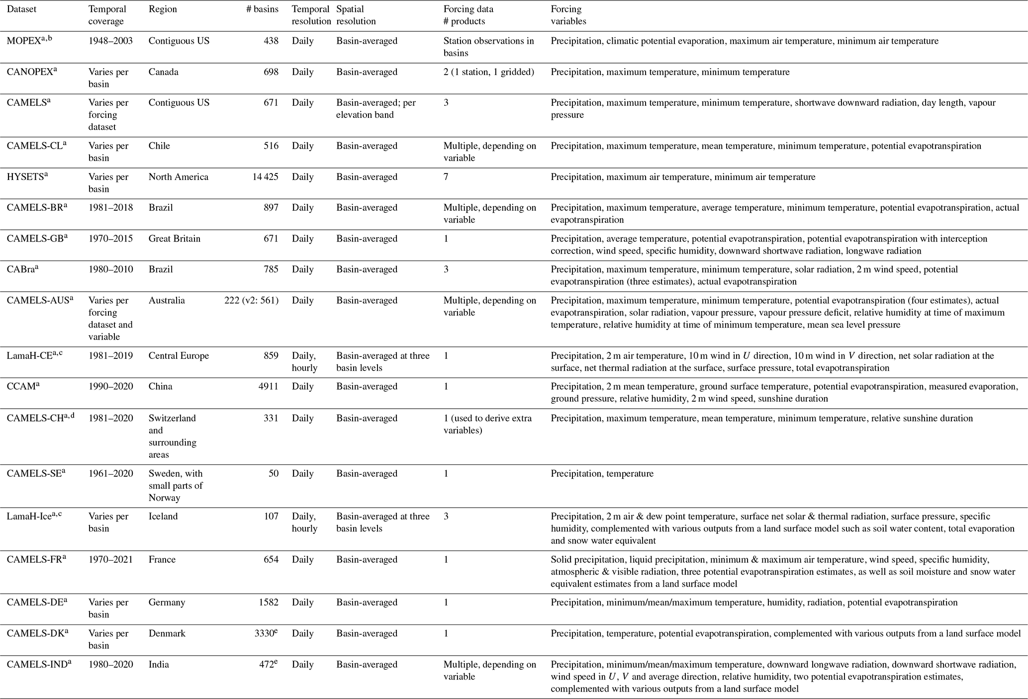
^a References: MOPEX (Schaake et al., 2006), CANOPEX (Arsenault et al., 2016), CAMELS (Newman et al., 2015; Addor et al., 2017a), CAMELS-CL (Alvarez-Garreton et al., 2018), HYSETS (Arsenault et al., 2020), CAMELS-BR (Chagas et al., 2020), CAMELS-GB (Coxon et al., 2020), CABra (Almagro et al., 2021), CAMELS-AUS (Fowler et al., 2021, 2025), LamaH-CE (Klingler et al., 2021), CCAM (Hao et al., 2021), CAMELS-CH (Höge et al., 2023), CAMELS-SE (Teutschbein, 2024), LamaH-Ice (Helgason and Nijssen, 2024), CAMELS-FR (Delaigue et al., 2024), CAMELS-DE (Loritz et al., 2024), CAMELS-DK (Liu et al., 2025), CAMELS-IND (Mangukiya et al., 2025).
^b MOPEX variables as described in the “basic requirements” in Duan et al. (2006).
^c LamaH-CE and LamaH-Ice basins are spatially connected.
^d CAMELS-CH forcing variables derived from the core forcing include precipitation, mean temperature, global radiation, sunshine duration, wind speed, relative humidity, potential evapotranspiration, actual evapotranspiration and intercepted evapotranspiration.
^e CAMELS-DK provides streamflow observations for 304 out of 3330 basins; CAMELS-IND provides streamflow observations for 228 out of 472 basins.

2 Design considerations and outcomes

Our goal with this dataset is to enable studies that investigate spatial heterogeneity across a wide variety of catchments, with a specific focus on spatially distributed process-based modelling. We also envision this dataset to be used to compare the performance of these models to their more empirical counterparts and for analyses not directly based on hydrologic models. Consequently, we processed a variety of data sources at various levels. We provide further detail about these requirements in the following subsections, as needed. Our general methodology for creating CAMELS-SPAT is as follows:

1. Define an initial set of basins of potential interest, covering the US and Canada;

2. Create consistent basin delineations for all basins identified under (1);

3. Obtain and process streamflow observations for the basins identified under (1), removing those basins for which no streamflow data can be found;

4. Obtain and process meteorological forcing data for the basins identified under (3);

5. Obtain and process geospatial datasets (e.g. data describing each basin's climate, vegetation, land use, topography, soil and geology) for the basins identified under (3);

6. Remove a number of very large basins from the basins identified under (3) and divide the remaining basins into various sub-datasets, based on disk space considerations;

7. Calculate catchment attributes using the data processed under (3), (4) and (5).

Figure 1 shows a visual summary of the main steps and decision points in this process, and each step is explained in more detail in the following subsections. For the reader's benefit, we present combined descriptions of the methods and results for each of these steps in the following seven subsections, instead of splitting these into dedicated Methods and Results sections. The code used to generate this dataset is available online (see the “Code and data availability” statement).

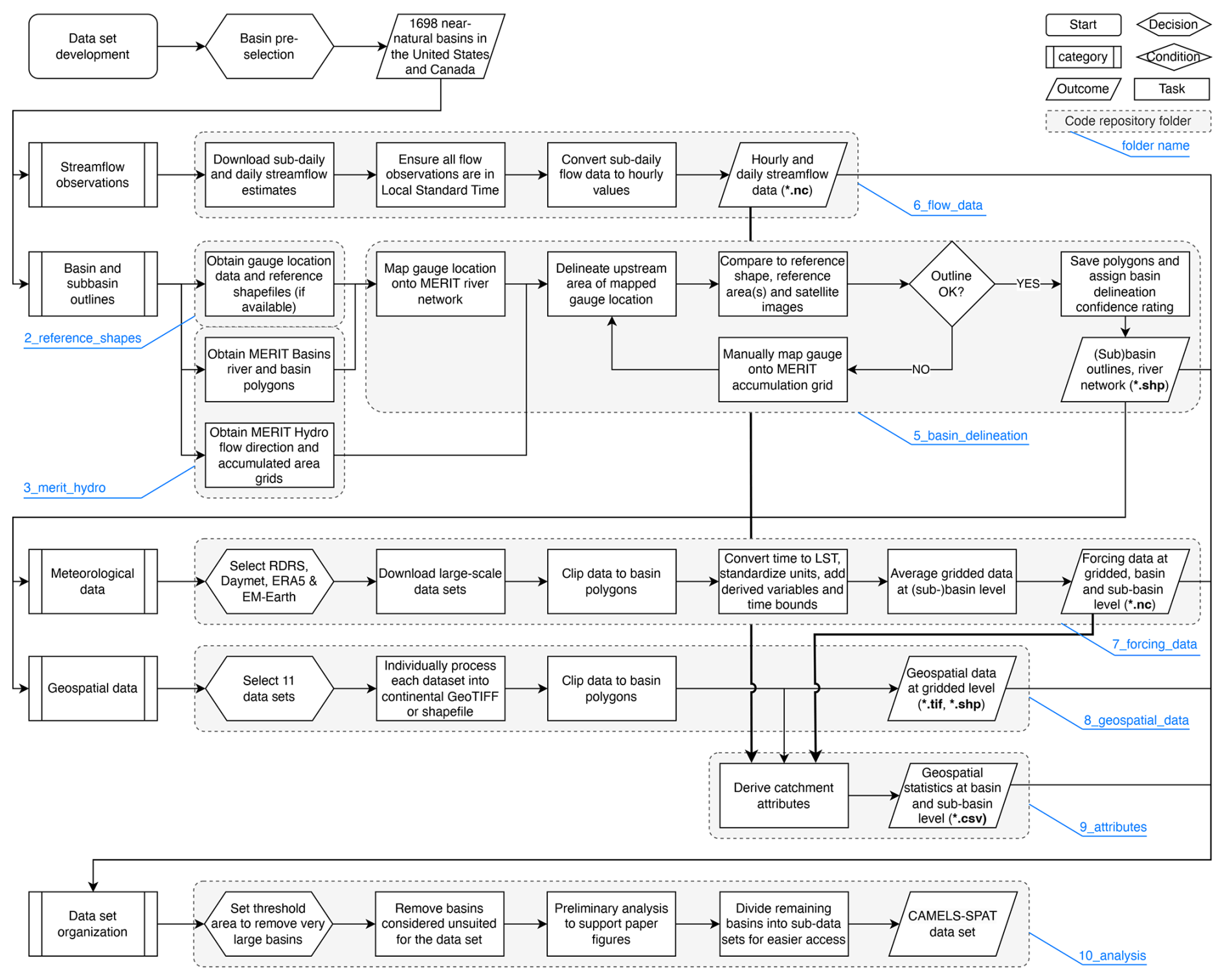
Figure 1 Overview of the CAMELS-SPAT workflow. Grey boxes and light-blue call-outs indicate specific folders on the GitHub repository, where the necessary code to reproduce these steps can be found. Note that the repository folder 4_data_structure_prep is not listed in this figure because it contains no methodological choices.

2.1 Basin pre-selection

2.1.1 Context

We impose two initial constraints on the basins we will consider including in this dataset. First, we have chosen to focus this dataset on (near-)natural basins. Human impacts on the earth system are critically important but substantially complicate hydrologic behaviour and are typically difficult to quantify and thus difficult to account for during analyses. Such impacts include but are not limited to (i) the construction of water management structures such as dams and drainage ditches at the local level, of which the location and size are difficult to ascertain and usually unreported in the continental-scale datasets that CAMELS-SPAT relies on; (ii) the construction of large water management infrastructure such as diversions and reservoirs, which may appear in continental-scale datasets but for which operating procedures are typically unknown; and (iii) surface and groundwater abstractions (e.g. agricultural and industrial use), for which abstraction and return volumes are typically unknown. That said, it is almost unavoidable that any selected basin includes at least some human impacts (tourism/recreation, drainage, forest management, etc.). We rely on existing classifications to select basins that are closer to the natural end of this continuum. Second, we require the availability of at least some streamflow observations at a sub-daily resolution. Process-based models are typically run at sub-daily time steps to more accurately simulate diurnal variation in processes such as evaporation, transpiration, sublimation and snow melt. In certain basins, such diurnal variability is visible in the streamflow record, and sub-daily observations are necessary to evaluate the appropriateness of process-based model equations. Daily data are by definition too coarse to distinguish such patterns.

2.1.2 Methods and outcomes

For basins in the US, we rely on the basin selection made by Newman et al. (2015) that was used for the CAMELS dataset (Addor et al., 2017a). This ensures that some level of comparison between outcomes of studies using either CAMELS or CAMELS-SPAT is possible. We refer the reader to Sect. 2.1 in Newman et al. (2015) for a description of the criteria used to create this selection of 671 basins, and note that, despite meeting these criteria, no basins in Alaska, Hawaii or Puerto Rico were included in the original CAMELS dataset due to limited spatial coverage of the Daymet data at the time. Our primary forcing dataset (see Sect. 2.4) does not have the coverage to include basins in Hawaii or Puerto Rico, but cold region processes as may be found in Alaska are covered by our selection of Canadian basins.

For basins in Canada, we start with the list of 1027 gauges included in the “Reference Hydrometric Basin Network” (RHBN; Environment and Climate Change Canada, 2020a, retrieved: 18 August 2022). These gauges have a minimum data availability of 20 years and minimal anthropogenic impacts as quantified by the presence of agriculture, built-up areas and water management infrastructure, as well as population and road density. These criteria are comparable to those described in Newman et al. (2015). Note that agriculture presence in the Canadian prairie provinces (Alberta, Saskatchewan, Manitoba) and southern Ontario is substantial and above the 10 % area threshold used for the other provinces and territories (Pellerin and Nzokou Tanekou, 2020, p. 7). Excluding these basins would severely reduce the number of Canadian gauges we could include in the dataset, and we thus retain these gauges but include various data products in CAMELS-SPAT that can be used to quantify or filter by the presence of agriculture.

Our initial basin selection included 1698 basins across the US and Canada. Various basins had to be removed due a lack of streamflow estimates or sub-daily data (see Sect. 2.3). We further removed several of the largest basins from the dataset, under the assumption that any new insights that could be gained from these extremely large basins are minimal (especially given that these basins are severely under-gauged for their size) and do not outweigh the extra disk space needed to store the data for these basins (see Sect. S3 in the Supplement for details). Our final selection consists of 1426 basins, with an approximately even spread between the US and Canada. For clarity, any outcomes shown in Sects. 2.2 to 4.4 only show the final 1426 basins we have made publicly available, rather than the 1698 basins that are the outcome of this basin pre-selection step.

2.2 Basin delineation

2.2.1 Context

Hydrologic datasets such as this are conditional on having accurate basin outlines. Basin outlines are used to estimate a drainage basin's area, to crop meteorological and geospatial data to the area of interest and to define the spatial extent of model configurations. Basin area estimates are also often used to convert the units of fluxes from volume-per-time to depth-per-time or vice versa (e.g. from m³ s⁻¹ to mm s⁻¹). Using incorrect basin area estimates can lead to large conversion errors that propagate into any further analysis (McMillan et al., 2023).

The basin polygons provided as part of the CAMELS data (Newman et al., 2014; Addor et al., 2017b) are administrative boundaries. These polygons are not based on gauge locations, and the polygons thus tend to overestimate the basins' drainage areas. Estimated area errors (derived from a comparison of reported upstream area for each gauge and actual area of the basin polygon) are typically in the order of some percent (below 2 % for approximately 70 % of basins) but can be substantial (above 10 % for approximately 8.5 % of basins, with individual cases well above 100 %). Additionally, openly available polygons for the Canadian gauges did at the time of project initialization not fully cover all 1027 basins listed in the Reference Hydrometric Basin Network (RHBN) (Environment and Climate Change Canada, 2020b, retrieved: 31 January 2022).

To address both concerns, we delineated new basin outlines for all basins identified as potential candidates in Sect. 2.1. Our specific goals were to (1) identify the upstream area of each gauge and (2) divide this upstream area into sub-basin polygons of roughly equal size.

2.2.2 Method and outcomes

We obtained gauge metadata (location, name, reference areas, etc.), as well as reference basin outline polygons if these were available, for all gauges identified in the first step. For the US gauges, metadata and polygons showing each basin's outline were obtained from the CAMELS dataset (Newman et al., 2014; Addor et al., 2017b). For the Canadian gauges, an initial download of the RHBN metadata was used to identify which gauges are included in the RHBN version released in 2020. Further metadata (location, name) were then extracted from the HYDAT database (Environment and Climate Change Canada, 2010). Two different sets of reference polygons were available (Environment and Climate Change Canada, 2020b; Government of Canada, 2022, accessed: 23 August 2022, 18 August 2022, respectively), of which we preferentially used the newer polygons if these were available for our basins of interest.

To divide larger basins into smaller sub-basins, we used the MERIT Basins dataset (Lin et al., 2019). This dataset contains vectorized river basins and river networks, derived from the MERIT Hydro data (Yamazaki et al., 2019). The mean sub-basin size in the MERIT Basins data is 45.6 km² (median: 36.8 km²). We refer the reader to Lin et al. (2019) for further details. We also obtained the MERIT Hydro flow direction and accumulation grids (Yamazaki et al., 2019). The MERIT Hydro data are provided as gridded data in a regular longitude/latitude coordinate system (EPSG:4326). This is a common format (most of the meteorological data, and many of the geospatial datasets we discuss in Sect. 2.4 and 2.5 are also only available in EPSG:4326). We adopt this as the standard in CAMELS-SPAT to the extent feasible. The one exception is the RDRS meteorological dataset, which is originally provided on a custom rotated latitude/longitude grid. Any area calculations and certain shapefile intersection operations are performed in the North America Albers Equal Area Conic projection (ESRI:102008).

The MERIT Basin network was derived independently from gauges, and the sub-basins in this dataset therefore do not align with gauge locations as reported by the U.S. Geological Survey and the Water Survey of Canada. For a given basin, we thus needed to clip the most downstream sub-basin polygon to the gauge. We therefore first mapped the gauge locations onto the MERIT Hydro river network using automated techniques. This mapping is intended to guarantee that the delineation of the upstream area of a given gauge starts from a pixel in the flow direction grid that is part of the main river (rather than the most downhill pixel of a single hillslope). However, there are various scenarios where automatic mapping is inaccurate and manual intervention is needed. We identified those cases through a combination of accuracy metrics (area comparison between new basin delineation and reported reference area(s) as well as percentage overlap between new basin delineation and reference polygon if any were available) and visual inspection of the new basin delineation, reference polygon, underlying MERIT Hydro data grids and satellite images. If necessary, we manually defined a better outlet location to delineate the basin from and tracked this intervention in the CAMELS-SPAT metadata. We also assigned confidence ratings to our new basin polygons based on these quality assurance checks. As the final step, we identified all cases of nested gauges where a larger basin includes a smaller one. In such cases, we split the sub-basin polygon that contains the nested gauge and assigned unique identifiers to the upstream and downstream parts of the sub-basin and river segment.

Figure 2 shows the resulting polygons for the 1426 basins that form the final CAMELS-SPAT dataset, with colours indicating the confidence ratings we assigned based on the checks listed previously (i.e. automated overlap and area checks, as well as manual inspection of polygons and satellite images). “Unknown” refers to cases where no confidence rating could be assigned, mainly due to lacking reference polygons. “Low” ratings are assigned when evidence suggests that our basin delineations are inaccurate, and we were unable to manually find a better outlet location that would lead to improved basin outlines. “Medium” ratings indicate that there are substantial differences between our new delineations and existing ones and/or reference areas but that it is difficult to decide whether our new delineation or the reference(s) are more accurate. “High” ratings are assigned when there is a clear match between our new polygons and the reference(s) or when evidence suggests our new delineations are more accurate than the reference(s). Detailed reasons for these ratings are tracked as part of the CAMELS-SPAT metadata. Medium and low confidence ratings occur primarily in regions with flat topography where finding the true outline of any drainage basin is difficult.

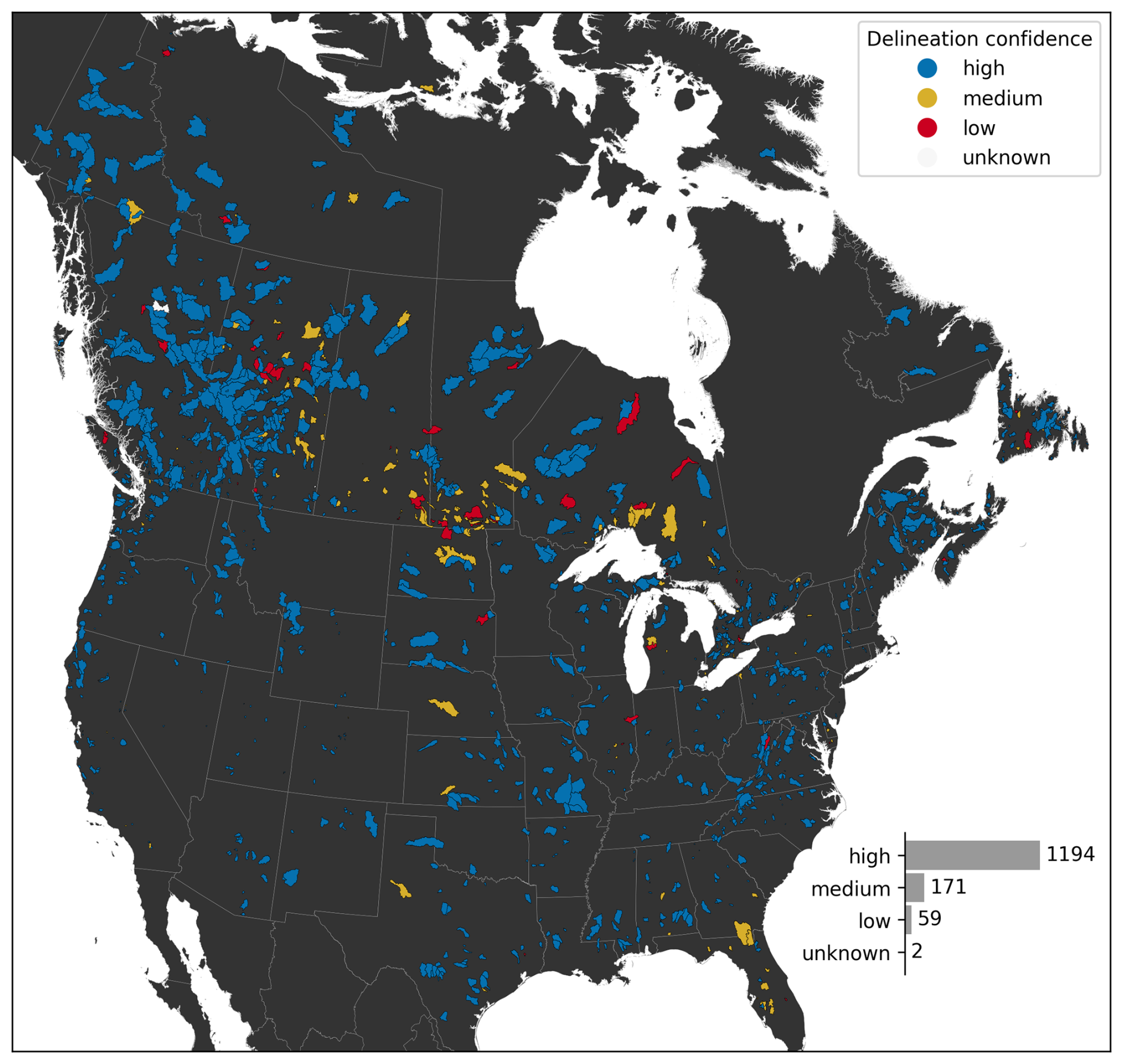
Figure 2 Location and delineation confidence of 1426 CAMELS-SPAT basins. Political boundaries by the Commission for Environmental Cooperation (2022, last access: 20 December 2023).

2.3 Streamflow observations

2.3.1 Context

Streamflow is a key variable for many hydrologic studies. Streamflow estimates are typically provided as either instantaneous values (i.e. valid at a given point in time) or as averages over a given time interval. It is critical to know what type of values (instantaneous or time averages) are available, as well as the time zones that the data are provided in.

The U.S. Geological Survey (USGS) typically collects instantaneous streamflow observations at 15 or 60 min intervals. USGS also provides daily average values, computed from the instantaneous data from 00:00 to 24:00 local standard time (LST; USGS, personal communication, 20 June 2023). Both instantaneous values and daily averages are publicly available.

The Water Survey of Canada (WSC) typically collects instantaneous streamflow observations at 5 min intervals and from these calculates daily averages that are reported in LST through the HYDAT database (WSC, personal communication, 4 July 2023). However, when instantaneous values are extracted through the WSC API, the time series are converted to coordinated universal time (UTC) before being given to the user (Government of Canada, 2023). Instantaneous streamflow observations are available through this API for the period between the present and minus 18 months. Recently, WSC has also released sub-daily data going back to 2011 (last access: 2 June 2025, Water Survey of Canada, 2025), although this cannot be accessed through the standard API. To expand the hourly data availability for Canadian basins, we included this data source in our processing. Daily average values are available for the full time period for which a gauge has been active.

Our goal with this project is to provide data that are useful for running and evaluating process-based hydrological models. We therefore include daily average streamflow values as available through USGS and WSC. We also include hourly average streamflow values to match the temporal resolution of our selected meteorological datasets. Hourly average flow data are computed from the sub-daily instantaneous data available through both agencies. All flow data, as well as meteorological forcing data, are included in the CAMELS-SPAT dataset in local standard time. The time zone of each gauge is tracked as part of the metadata.

2.3.2 Method and outcomes

For the gauges in the US, daily average streamflow data and instantaneous (sub-daily) data can both be extracted through API requests (https://nwis.waterservices.usgs.gov/nwis/dv/ and https://nwis.waterservices.usgs.gov/nwis/iv/, respectively; last access: 16 June 2023). For the Canadian gauges, sub-daily data were extracted from the Environment and Climate Change Canada FTP server (https://collaboration.cmc.ec.gc.ca/cmc/hydrometrics/www/UnitValueData/, last access: 31 May 2025). Daily data were extracted from the HYDAT database, version 20230505. We excluded four gauges in the US and 180 Canadian gauges from the original 1697 pre-selected stations because sub-daily data were not available for these stations. We removed a further 13 Canadian gauges for lacking daily discharge values. Manual checks of these gauges through the WSC website (https://wateroffice.ec.gc.ca/search/historical_e.html, last access: 6 February 2025) indicate that these stations measure water levels in lakes.

Daily average values for both countries are provided in LST. We updated the time indices for the sub-daily instantaneous values to match. For the gauges in the US, this meant shifting the time series by 1 h for time steps that were provided in local daylight saving time for gauges in states where daylight saving time is observed. For the Canadian gauges, this meant shifting the entire time series for each gauge by the offset needed to convert UTC to LST. We then set any negative streamflow values to zero and used a mass-conserving averaging approach to turn instantaneous flow data into hourly averages (see Sect. S1 in the Supplement for more details about the averaging procedure). We specified the condition that every hourly average must be based on at least one observation during that time window. Hours for which no data observations were available were set to not-a-number (NaN).

Note the critical assumption that we calculated the average hourly flows as the value at the top of the hour (e.g. 12:00) using a forward-looking window (in this case, the value at 12:00 is the average during the time window 12:00–13:00). This matches the daily flows, which are provided under the same assumption by USGS and WSC (e.g. the 1 January 2000 value is calculated from data between 00:00, 1 January and 24:00, 1 January; USGS, personal communication, 20 June 2023; WSC, personal communication, 26 June 2023). This information is also stored in the time_bnds (time bounds) variable available in the provided NetCDF files.

Daily and sub-daily observations were originally provided in text-based formats. We converted these to NetCDF4 formats to ensure consistency between gauges in the two countries and to track metadata in a more accessible way (compared to storing the metadata in separate files or headers in text files). For both USGS and WSC data, we retained the quality flags that accompany the data and stored these in the same NetCDF files that contain the streamflow observations. These quality flags indicate conditions that may adversely affect the observations (e.g. gauge malfunction, ice conditions) and whether data have been formally approved or are still considered provisional.

Figure 3 shows aggregated flow data availability for the 1426 catchments included in the CAMELS-SPAT dataset, with the total record length in blue (number of years between first and last available streamflow observation) and missing values in red (number of years in the record length for which no observations are available). Hourly flow data come in two distinct categories: records for the Canadian gauges are around a decade in length, while sub-daily records for gauges in the US are typically two to three times longer. This is a consequence of the Water Survey of Canada's policy to make high-resolution gauge data publicly available for only a relatively short historical period. Missing data for these shorter records are, however, typically low (see also Fig. A1). For approximately 60 % of gauges, missing hourly observations account for up to 10 % of the record length. Data may be missing for up to 40 % of the record for most remaining gauges, with a handful of gauges having extremely large data gaps. Daily data record lengths are similar for Canadian and US gauges. Missing values are relatively rare (<1 % for up to 849 out of our 1426 gauges and <10 % for 1070 out of 1426 gauges), although this can be substantial (up to approximately 60 %; see Fig. A1). The period with the greatest overlap of data records is 1990–2020; hourly observations are available for only a handful of gauges before this time. Some further statistics on the streamflow regimes available in CAMELS-SPAT are discussed in Sect. 3.5.

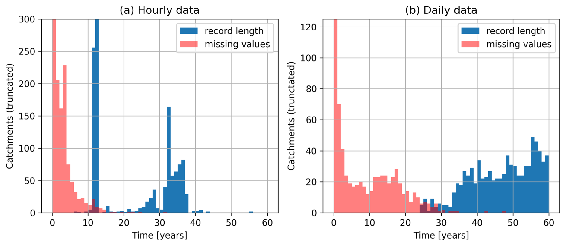
Figure 3 Flow data availability for gauges included in CAMELS-SPAT. Record length refers to the period between the first publicly available flow record for a given station and its last. Missing values occur in this record period and are given here in the same units as the record length itself. Note that both y axes are truncated: in (a), there are 556 cases where the number of missing values falls between 0 and 1 years of total (although note that these missing values are not necessarily consecutive and in fact in many cases are caused by seasonally active gauges). Also truncated is the record length bar showing the 498 cases where the length of the hourly data record is between 12 and 13 years. In (b), missing values has a count of 898 for time between 0 and 1 years. (a, b) Note that the colours are partly transparent and that overlaps between the record length and missing values bars will appear as dark red.

2.4 Forcing data

2.4.1 Context

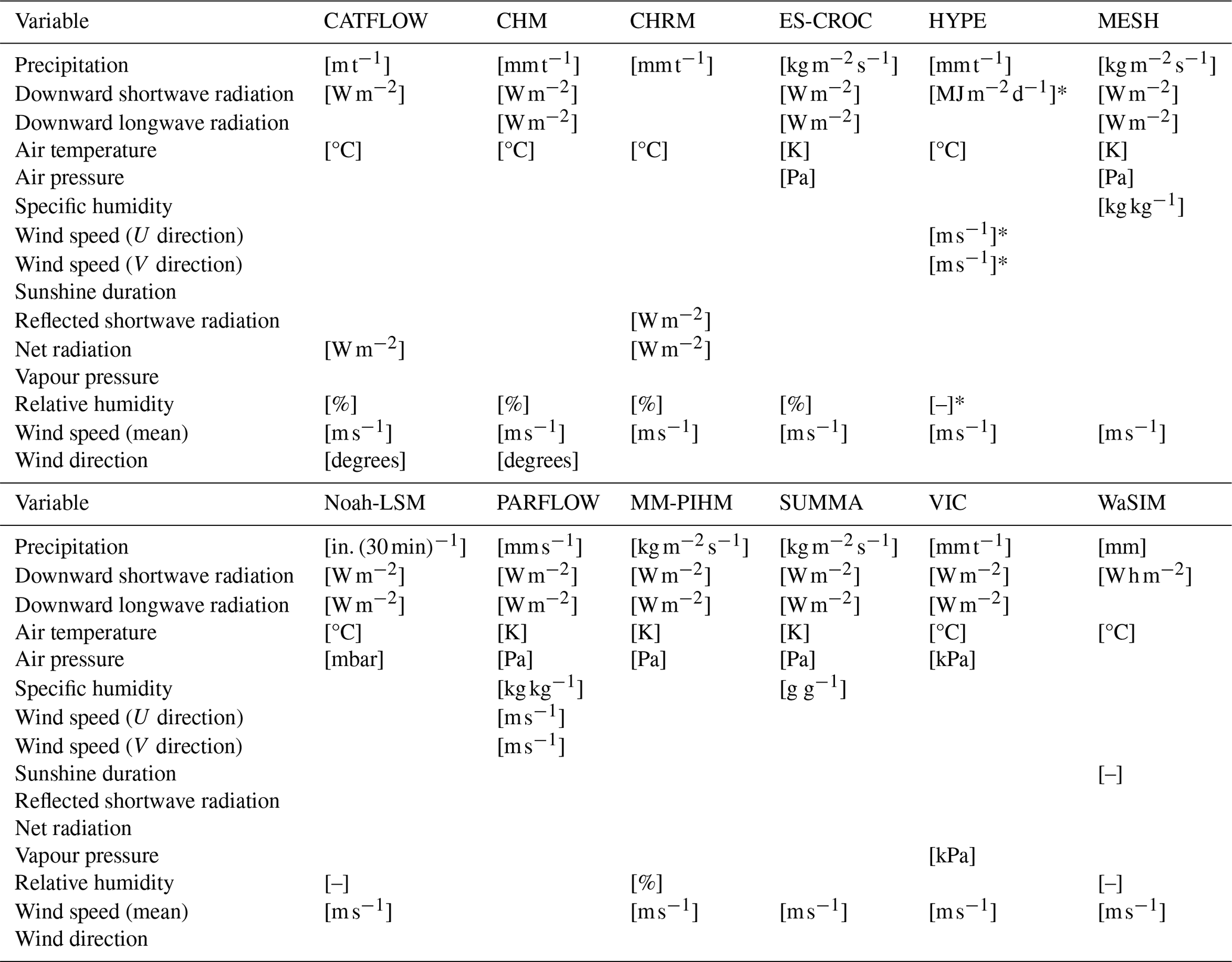
Meteorological forcing data in existing datasets are typically provided as catchment-averaged (lumped) daily data and tends to be limited to precipitation, temperature and potential evapotranspiration variables (Table 1). While a large number of the more conceptual models can be run with only precipitation, temperature and potential evapotranspiration inputs (see e.g. Knoben et al., 2019; Trotter et al., 2022), more complex hydrologic models typically require a wider array of inputs at a higher temporal resolution. Table 2 shows a brief overview of the meteorological data requirements for a selection of process-based hydrological models. Typical variables include (1) precipitation, (2) air temperature, (3) radiation (often distinguishing between shortwave and longwave radiation), (4) air pressure, (5) humidity and (6) wind speed.

It is clear from Table 2 that it is impossible to define a small set of forcing variables that would allow the use of a large number of process-based hydrologic models. We therefore decided to include a broad selection of meteorological variables, accepting that this comes at the cost of extra disk space. We provide these variables at hourly time steps, at their original gridded resolution as well as averaged at the sub-basin level. To facilitate the use of the broadest range of modelling tools, we also include time series of potential evaporation (see footnote in Table 3) and forcing variables aggregated at the lumped basin level.

Table 2 Meteorological data needs for CATFLOW (Maurer and Zehe, 2007), CHM (Marsh et al., 2020), CHRM (Pomeroy et al., 2007), ES-CROC (Lafaysse et al., 2017), HYPE (SMHI, 2022), MESH (Mekonnen and Brauner, 2020), Noah-LSM (Mitchell et al., 2005), PARFLOW (Maxwell et al., 2019), MM-PIHM (PIHM team, 2007; Yuning Shi, 2018), SUMMA (Clark et al., 2015a, b; Nijssen, 2017), VIC (Liang et al., 1994; Hamman et al., 2018) and WaSIM (Schulla, 2021). Models are listed alphabetically. Optional inputs indicated with *. t indicates an arbitrary time unit.

2.4.2 Methods and outcomes

CAMELS-SPAT includes four forcing datasets, each with a specific focus:

1. First, we primarily use the high-resolution RDRS v2.1 dataset (Gasset et al., 2021, available at 10 km or approximately 0.09° resolution). RDRS covers the North American continent and provides those variables needed to run process-based models directly and derive most other variables listed in Table 2. A key advantage of RDRS is that it assimilates precipitation observations, which should improve the accuracy of its precipitation field.

2. Second, for continuity with the original CAMELS dataset, we include the Daymet v4 R1 dataset (Thornton et al., 2021, available at a 1 km or approximately 0.009° resolution). Daymet is based on weather station observations and gridded terrain data and is available at a daily resolution between 1980 and 2023 on a 365 d calendar (during leap years, 31 December is missing). The dataset does not include all the forcing variables needed to run process-based models but, if combined with an appropriate estimate of potential evapotranspiration (PET), provides sufficient information to run more conceptual and data-driven models. We infill the missing day in leap years as a linearly interpolated value between the preceding and following days. Following Newman et al. (2015), we add a Priestley–Taylor PET estimate (Priestley and Taylor, 1972, further details available in Sect. S2.5 in the Supplement).

3. Third, to facilitate possible extension of CAMELS-SPAT beyond North America, as well as provide hourly data for gauges with observations before 1980 (i.e. outside the time period covered by RDRS), we include the globally available ERA5 data (Hersbach et al., 2020, available at a 0.25° resolution). Like RDRS, ERA5 provides all variables needed to run process-based models directly and derive most other variables listed in Table 2. However, unlike the other datasets listed here, ERA5 is a reanalysis product and does not integrate station observations. Local accuracy may thus be lower for ERA5 data than for datasets that do use station observations.

4. Fourth, to partly address this weakness of ERA5 data, we include the high-resolution EM-Earth dataset (Tang et al., 2022b, available at a 0.10° resolution). Previous work has shown that using station-based precipitation and temperature data from EM-Earth provides better modelling results for the North American continent than using ERA5 alone (Rakovec et al., 2023). However, note that EM-Earth has a fixed temporal coverage of 1950–2019, whereas our selected gauges have data beyond 2019.

Table 3 shows an overview of forcing variables available as time series in the CAMELS-SPAT dataset. Compared to Table 2, we provide net radiation terms at the surface separated into net shortwave and net longwave terms and do not provide a summed net radiation component or a reflected shortwave variable. Either can be easily derived from the provided net shortwave and longwave components (see Hogan, 2015, but also footnote ^b in Table 3). We also do not provide sunshine duration because this is not available in RDRS, Daymet and EM-Earth. While sunshine duration is available in ERA5, it is not an independent variable: it is derived directly from downward shortwave radiation using a threshold of 120 W m⁻² (Hogan, 2015). We complement the forcing datasets with various additional variables derived from the downloaded data in cases where we judged the processing to be too cumbersome to pass down to the user (i.e. vapour pressure, relative humidity, wind direction) or where the variable seemed to be of general interest (i.e. mean wind speed, PET). Potential evapotranspiration estimates for Daymet were derived using the Priestley–Taylor formula (Priestley and Taylor, 1972); PET estimates for RDRS were derived using the FOA-56 Penman–Monteith method (Allen et al., 1998). The equations used to derive data are provided in Sect. S2 in the Supplement. While the list of variables in Table 3 is unlikely to completely cover all models' data needs, it will provide a reasonable starting point for a large number of models.

We retained the original variable names used in each dataset so that users may easily refer to the existing documentation of RDRS, Daymet, ERA5 and EM-Earth if needed. For convenience and simplicity from a user perspective, we converted all hourly data to use a consistent set of units, although we kept the units of the daily data (Daymet) to be more directly applicable to the types of models more commonly run at daily time steps. Unit conversion of hourly data is mostly straightforward but required an assumption for the density of water, which we set at a constant value of 1000 kg m⁻³. Data are provided for the full time period covered by the observational record of each individual gauge when possible, including time steps for which streamflow data are missing (see also Sect. 4.2.2 and Table 4). For all variables, metadata (descriptions, units, derivations if applicable) are stored as variable attributes in the NetCDF files.

We provide the forcing data at three different spatial aggregation levels: (1) as gridded values at the original spatial resolution of each dataset, clipped to the basin outline; (2) aggregated at the sub-basin level; and (3) aggregated at the basin level (i.e. the level at which most of the datasets listed in Table 1 provide data). Averaging of the gridded data to (sub-)basin polygons was done with the EASYMORE toolbox (Gharari et al., 2023).

RDRS, ERA5 and EM-Earth provide data at an hourly resolution, in coordinated universal time (UTC). We process these time indices to be in each gauge's local standard time (LST) instead, so that the time indices in the forcing file align with those used for the flow observations. We make a slight adjustment for the 57 basins that are located in regions following Newfoundland standard time (NST [UTC−3 h 30]; National Research Council Canada, 2019). The time series of all forcing data products only provide values at the top of each hour (12:00, 01:00, etc.) and thus cannot easily be converted to NST without making assumptions about how to interpolate the data between the times for which they are available. We treat these basins as following Atlantic standard time (AST [UTC−4 h 00]) instead. Note that this leads to a 30 min offset between forcing data and streamflow observations for these basins. Daymet data are already provided as daily average values calculated in LST and require no further adjustment.

Variables in these forcing datasets are either instantaneous (i.e. representative of conditions at a specific point in time) or time averaged (i.e. representative of conditions over a given time window), and this means that the time stamps in each NetCDF file must be interpreted differently for different variables. For any instantaneous variable, a value is valid at the specific moment in time given by the time stamp (European Centre for Medium-range Weather Forecasting, 2023c). For any time-averaged variables, we need to distinguish between two cases. RDRS and ERA5 use period-ending or backward-looking time stamps, meaning that, for example, the average precipitation rate at time 12:00 is the average rate over the interval 11:00–12:00 (ECCC, personal communication, 2024; European Centre for Medium-range Weather Forecasting, 2023b, Sect. “Mean rates/fluxes and accumulations”). EM-Earth's precipitation variable instead uses period-beginning or forward-looking time stamps, meaning that, for example, the average precipitation rate at time 12:00 is the average rate over the interval 12:00–13:00 (Guoqiang Tang, personal communication, 2024). Table 3 provides an overview of all forcing variables and summarizes this information.

Table 3 CAMELS-SPAT meteorological variables. Variable names shown in bold indicate derived variables. “Flux validity” indicates how time-averaged variables must be interpreted.

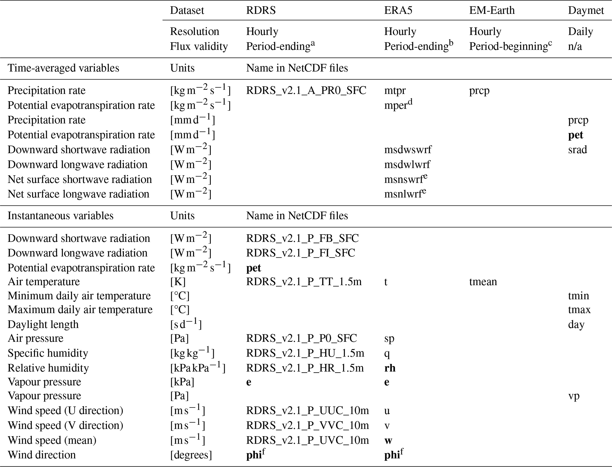
^a ECCC, personal communication, 2024. ^b See https://confluence.ecmwf.int/pages/viewpage.action?pageId=82870405#ERA5:datadocumentation-Table4 (last access: 3 January 2024), https://confluence.ecmwf.int/pages/viewpage.action?pageId=82870405#ERA5:datadocumentation-Table9 (last access: 3 January 2024), https://confluence.ecmwf.int/pages/viewpage.action?pageId=82870405#ERA5:datadocumentation-Table2 (last access: 3 January 2024). ^c Guoqiang Tang, personal communication, 2024. ^d Assumptions underlying this variable are described here: https://codes.ecmwf.int/grib/param-db/?id=228251 (last access: 1 January 2024). Note that we provide the equivalent variable as a mean rate as part of the CAMELS-SPAT data, but the URL for that variable lacks a clear description: https://codes.ecmwf.int/grib/param-db/?id=235070 (last access: 1 January 2024). ^e Note that these net radiation terms are based on interactions between the atmospheric and land surface components of the ERA5 modelling chain and should thus only be used carefully as a model input to prevent cases where the user's model duplicates processes already accounted for by the ERA5 models. ^f We derived most additional variables before averaging the gridded data onto (sub-)basins, but this is not easily possible for wind direction. Instead, we calculate wind direction separately for the gridded, semi-distributed and lumped cases from U and V components after (sub-)basin averages of these variables were created. We use the meteorological wind direction as defined by ECMWF (European Centre for Medium-range Weather Forecasting, 2023a): wind direction in this case indicates the direction that the wind comes from, not where it goes. n/a: not applicable.

2.5 Geospatial data

2.5.1 Context

Geospatial data in existing datasets cover four broad categories: (1) meteorology (as time series and derived summary statistics), (2) vegetation and land use, (3) topography and (4) soil and geology. In current large-sample datasets, geospatial data are typically not provided as maps in their original formats but tend to be presented as spatial statistics (mean, mode, etc.). These statistical summaries of the original data, commonly referred to as catchment attributes, can be helpful to succinctly characterize a location's hydroclimatic conditions and support classification efforts. For modelling purposes, geospatial data play a key role in defining model configurations and parameter values. For example, models such as Noah-LSM (Niu et al., 2011) and SUMMA (Clark et al., 2015a, b) rely on vegetation and soil classes to provide initial values for a number of land use and soil parameters. More generally, models might require the height of the vegetation canopy in the vertical direction or the fraction of the basin covered by open water in the horizontal direction as inputs. It is practically impossible to cover all possible use cases through statistical summaries of the data (i.e. through attributes) alone, and we therefore provide the geospatial data as maps clipped to the basin outlines. The maps will allow users to derive model parameters and further catchment delineations (such as elevation zones or land cover polygons) and to derive additional catchment attributes if our existing selection of attributes does not cover a particular study's needs (see Sect. 3). Figure 4 shows an overview of the 11 different datasets we selected for use in CAMELS-SPAT.

2.5.2 Methods and outcomes

For internal consistency of the CAMELS-SPAT data, we selected various geospatial datasets that cover at least the US and Canada. The specific processing steps vary, but in general processing for each dataset involved downloading the data at continental or larger scales and clipping the data to the basin polygons (see Fig. 1). We also ensured that all geospatial maps are provided in a regular latitude/longitude coordinate system (EPSG:4326). Figure 4 provides an overview of the geospatial data layers, using a single basin as an example.

Climate. Long-term monthly means of several climate variables can be obtained from the WorldClim dataset (Fick and Hijmans, 2017). The advantage over calculating these means from gridded forcing data is WorldClim's much higher spatial resolution. Available variables are the long-term means computed from 30 years each, showing minimum, mean and maximum monthly temperature, as well as the monthly precipitation, solar radiation, wind speed and water vapour pressure. WorldClim's data licence does not allow the redistribution of their raw data but does allow the data to be used to calculate derived statistics and to redistribute those. We primarily use the WorldClim data to calculate various attributes that quantify the spatial heterogeneity in climatic conditions and include various maps of derived variables as part of CAMELS-SPAT.

Vegetation. Process-based hydrological models typically include explicit representations of vegetation cover in a catchment. CAMELS-SPAT includes two datasets from which vegetation parameters may be derived. First, we included the time series of leaf area index (LAI) observations, derived from MODIS satellite observations (Myneni et al., 2021, MCD15A2H.061). These observations are available at an 8 d temporal resolution and cover the period 4 July 2002 to 8 October 2023. Certain models may be able to ingest these maps directly or typical seasonal LAI patterns may be derived from them. In addition, we included estimates of forest height in 2000 and 2020 (Potapov et al., 2021, part of the Global Land Cover and Land Use Change, 2000–2020 data).

Land cover and land use. To further assist parametrization and classification efforts, we included three different products related to land cover and land use. First, the Landsat-Derived Global Rainfed and Irrigated-Cropland Product (LGRIP30; Thenkabail et al., 2021; Teluguntla et al., 2023) can be used to estimate the magnitude and type of agriculture practised in each basin. Second, we include a map of International Geosphere–Biosphere Programme (IGBP) land classes in each basin, derived from MODIS satellite observations (Friedl and Sulla-Menashe, 2022). Third, we include high-resolution Global Land Cover and Land Use 2019 maps (Hansen et al., 2022). This is very high-resolution data derived from Landsat satellite observations, used to classify the landscape into several broad categories (inland water, permanent snow and ice, cropland, built-up, terra firma and wetlands), with several of these consisting of subclasses based on build-up area extent and vegetation extent and height.

Open water. We include cut-outs of the HydroLAKES data (Messager et al., 2016) to quantify the extent, type and volumes of open water bodies in each basin. These data can be used to estimate each catchment's open water area, retention volumes and parametrization of reservoir and lake modules in hydrologic and/or routing models.

Topography. The MERIT Hydro digital elevation model (DEM) used for basin delineation (Yamazaki et al., 2019) is also part of the maps provided for each catchment. We used the DEM to derive separate maps of slope and aspect because of their hydrologic relevance. For both, the DEM was first re-projected into ESRI:102009 (NAD 1983 Lambert North America) to ensure consistency between horizontal and vertical units. We then calculated slope maps expressed as angles (i.e. degrees) and aspect maps in degrees indicating which direction a slope faces (with 0, 90, 180 and 270° being north-, east-, south- and west-facing slopes, respectively). Additional variables such as elevation bands may be derived from the DEM map, but due to the subjectivity involved in deciding where the boundaries between the elevation bands are, we have not done so. The DEM data may also be useful in applying elevation-dependent lapse rates to meteorologic variables.

Soil and geology. We provide maps from three different datasets to characterize each catchment's subsurface. First, SoilGrids 2.0 (Poggio et al., 2021) provides estimates of various soil properties (bulk density; percentage coarse fragments; organic carbon content; and sand, silt and clay percentages) at six different depths (0–5, 5–15, 15–30, 30–60, 60–100 and 100–200 cm). These maps are given for mean values but also for 5th, 50th and 95th percentiles and an uncertainty estimate. To match the geological attributes described later in this paragraph, we also derive porosity and conductivity estimates from the mean sand and clay values for each layer using the regression equations described by Cosby et al. (1984). However, SoilGrids data are estimated for depths up to 2 m everywhere, without taking into account the actual depth to bedrock of any location. Thus, second, we included maps from the Pelletier soil database (Pelletier et al., 2016a, b). These distinguish between uplands, valley bottoms and lowlands and provide estimates of the depths of soil, intact regolith and sedimentary deposits above unweathered bedrock. These variables may be used to set more realistic soil depths in models compared to a spatially uniform depth. Third, we include cut-outs from the GLHYMPS data (Gleeson et al., 2014; Gleeson, 2018) as polygons. Contained as attributes are estimates of geologic permeability and porosity, which may be used to parametrize models.

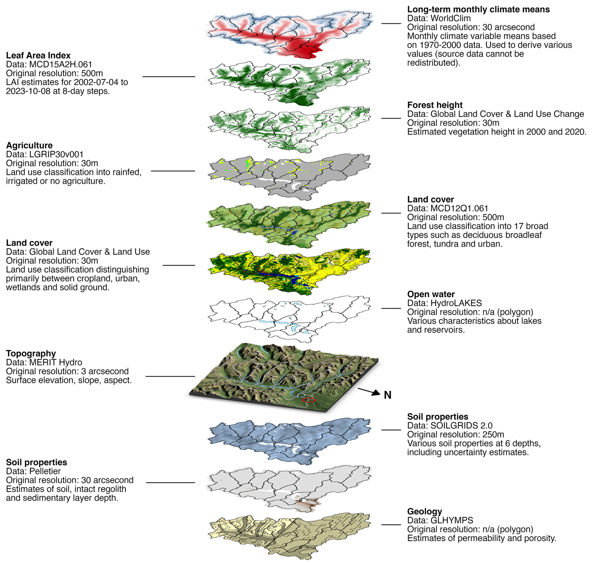
Figure 4 Overview of geospatial maps provided for each catchment in the CAMELS-SPAT dataset, using a transboundary basin as an example (Canadian gauge ID: 05AD003; sub-basin outlines given in black in all data layers apart from topography). The topography layer also shows the basin's gauge location as a red circle, the different sub-basins with white outlines and the river network and lakes in blue.

3 Catchment attributes

Existing large-sample datasets do not provide the maps of geospatial data that we include as part of CAMELS-SPAT (see Sect. 2.5) and instead provide only statistical summaries of such maps, known as catchment attributes (for example, a dataset might include the mean catchment elevation but not the DEM from which this mean elevation is calculated). An informal analysis of some of the CAMELS datasets listed in Table 1 shows that these datasets together contain close to 300 different attributes, although any given individual dataset contains no more than 50 to slightly over 100 of those. Overlap between attributes provided by existing datasets is moderate at best, partly as a consequence of the differences in data products included in each individual dataset. This lack of uniformity is compounded by a lack of unified terminology, where different datasets may use the same terms to describe different calculations or different terms to describe the same attribute. This is in line with findings by Tarasova et al. (2024), who analyse how 742 journal articles describe the hydroclimatic conditions of their study areas. They find that authors use a wide variety of attributes with only occasional verification of their attributes' usefulness. Relevant to our work, and in line with a cursory overview of attributes provided by the datasets listed in Table 1, they also find that the existing literature only rarely uses catchment descriptors that attempt to quantify the range a particular variable may cover in a given catchment (the CAMELS-SE dataset, Teutschbein, 2024, is a notable exception).

We thus made a necessarily subjective choice of which attributes to calculate for the CAMELS-SPAT basins. We aimed for overlap with existing datasets when possible and to be mindful of the findings of Tarasova et al. (2024). In particular, in addition to the commonly provided mean attribute values, we also selected statistics that describe the range of an attribute's values. Examples include the minimum, maximum and standard deviation of vegetation height to give an impression of the spatial variability in the forest height data and the inclusion of monthly mean forcing variables to give an impression of the climatic seasonality that is only superficially captured by average seasonality attributes commonly found in other datasets. A list of all 1178 attributes can be found in Tables A1–A11, divided into five main categories: (1) climate, (2) topography and open water, (3) vegetation and land cover, (4) subsurface and (5) hydrology. We calculate the attribute values at both the basin and the sub-basin level (except for streamflow statistics, which are only available at the basin outlet). Further details are provided in the following subsections, although for obvious reasons we do not discuss every individual attribute. Instead, we focus in the following description of the CAMELS-SPAT attributes on providing various examples that highlight why the recommendations in Tarasova et al. (2024) are important.

3.1 Climate attributes

The climatic data used in the development of CAMELS-SPAT, i.e. the time series of meteorological forcing variables from RDRS and the monthly maps of mean climatic conditions from WorldClim, provide a unique opportunity to characterize each catchment's climatic conditions in time and space. From the RDRS data, we are able to determine seasonal variability and its variance over multiple years. From the WorldClim data, we are able to characterize the seasonal variability and its variance across space. This leads to a relatively large number of climatic attributes compared to other datasets and provides some insight into the variability in time and space of this driver of hydrologic behaviour.

Tables A1–A4 list the climatic attributes provided with CAMELS-SPAT. These cover annual mean values of variables of interest (such as precipitation, potential evapotranspiration and snow) commonly found in other datasets, as well as standard deviations for these values. We expand upon existing datasets by also providing monthly means and monthly standard deviations of all forcing variables, to allow more in-depth investigation of each catchment's seasonality. Figure 5 shows why going beyond annual mean values may be important. Figure 5a and b show long-term average aridity and the fraction of precipitation falling as snow (determined on a per-time-step basis using a 0 °C threshold; see also Sect. 4.2.8 for some further discussion about the PET estimates available in CAMELS-SPAT.). The broad geographical patterns seen here are not particularly surprising but are, importantly, not necessarily representative of climatic variability on a year-to-year basis (Fig. 5c, d) or of the range of conditions in each catchment (Fig. 5e, f). For example, across the Great Plains area and particularly in the southwestern US, the year-to-year variability in aridity (Fig. 5c) can be quite large, and certain catchments may fluctuate between arid and humid states on annual timescales. The fraction of precipitation falling as snow equally shows large inter-annual variability (Fig. 5d), with standard deviations close to 10 % across a large part of the domain. Within-catchment variability of aridity (Fig. 5e) seems modest in most cases but is rather large for snowfall (Fig. 5f), highlighting why treating these catchments in a more spatially distributed fashion may be helpful.

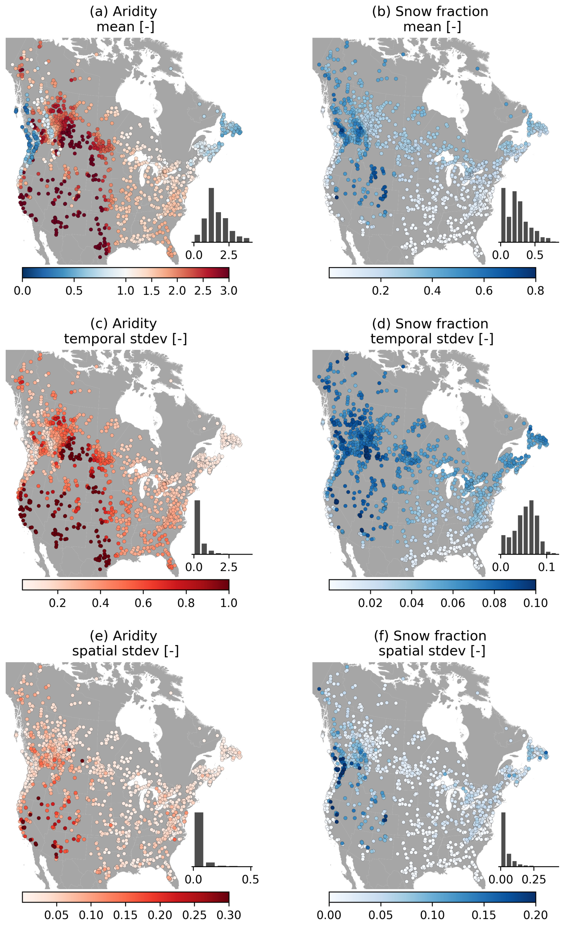
Figure 5 Selection of climate attributes. (a–d) Statistics derived from RDRS data, showing mean and variability in time. (e–f) Statistics derived from WorldClim data, showing variability in each catchment.

3.2 Topography and open water attributes

Topography is a critical control on hydrologic behaviour at both the large and the small scale. For example, mountains influence precipitation patterns at the large scale, while at the small scale, slope angles affect lateral drainage and topographic features can lead to the formation of lakes. Tables A5 and A6 provide an overview of topographic and open water attributes, respectively. These cover various basic catchment descriptors, such as location and area, and various statistics about the topography and resulting drainage network. Figure 6a and b show the catchment elevation mean and standard deviation, respectively. As expected, elevation varies strongly throughout the domain, ranging from sea level to well over 3000 m above sea level ($\mathrm{m}\mathrm{a}.\mathrm{s}.\mathrm{l}.$). Elevation differences in catchments can be very high in mountainous regions, with prime examples being the northwestern US and southwestern Canada: the within-catchment standard deviations in elevation are close to 500 m here. Statistics that quantify basin slope (not shown for brevity) show similar patterns, showing that the topographic drivers of hydrologic behaviour can be highly variable in catchments. Topographic conditions lead to a certain amount of open water in the CAMELS-SPAT catchments, with lakes larger than 0.1 km² being more prevalent in the Canadian basins (Fig. 6c) than in basins in the US. Water storage in these can be considerable (Fig. 6d). Stream lengths (Fig. 6e and f) vary considerably based on the drainage area upstream of each gauge, emphasizing a need for within-catchment routing approaches. The examples in Fig. 6 are intended to highlight the variability of conditions in catchments and thus emphasize the need to go beyond treating basins as lumped entities. These examples (particularly Fig. 6a, b, e and f) also illustrate that attributes can show high correlations, suggesting that adding more attributes to an analysis will not necessarily increase the useful information by the same amount. Selecting which attribute to incorporate in any analysis must thus be done somewhat carefully (see also Sect. 4.2.7).

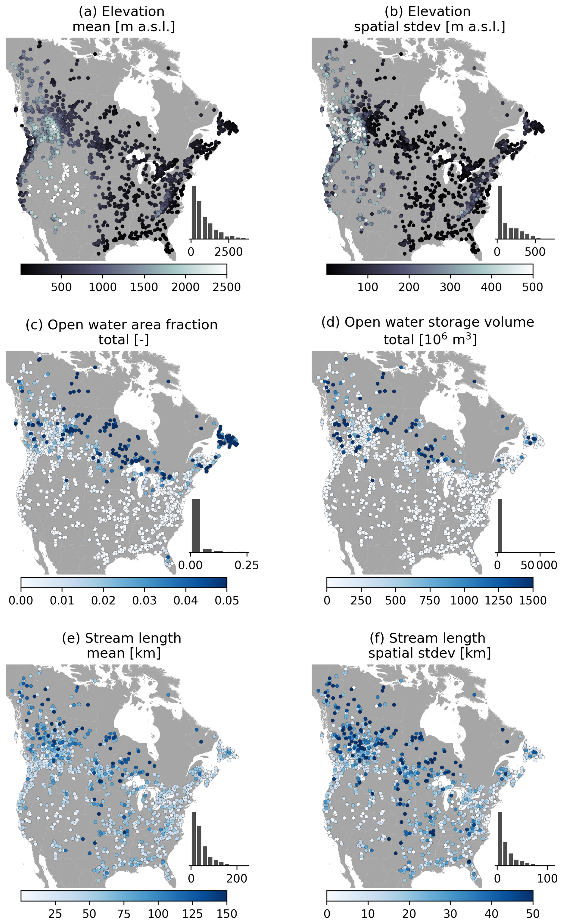
Figure 6 Selection of topographic attributes. Open water (c, d) estimates are obtained from the HydroLAKES database, which uses a threshold of 10 ha (0.1 km²) for lake and reservoir identification. (e, f) Stream length statistics are derived by starting at each headwater sub-basin upstream of a given gauge and tracing the flow path down until the gauge location is reached. From this ensemble of flow path lengths upstream of a given gauge, the mean and standard deviation of stream lengths are calculated.

3.3 Land cover attributes

Table A7 provides an overview of vegetation and land cover attributes. Briefly, these cover various statistics on vegetation height during specific years, monthly leaf area index (LAI) catchment mean and standard deviation, as well as per-catchment counts of three different land class products. We refer the reader to the original publications that describe each dataset for further information about the classes included. Figure 7 provides an example of the spatial (Fig. 7a, b) and temporal (Fig. 7c, d) variability in vegetation characteristics. As may be expected, there is considerable variation in vegetation height in space, on both the continental and within-catchment scale. Forested areas in particular exhibit large standard deviations in vegetation height (see for example the Pacific Northwest and western Canada). On a seasonal scale, LAI exhibits large variability throughout the domain as a consequence of summer and winter patterns. Vegetation is a key control on hydrologic processes like interception and transpiration, and these images show that mean attribute values alone do not necessarily capture the complex vegetation patterns that may explain spatial and temporal variability in these processes.

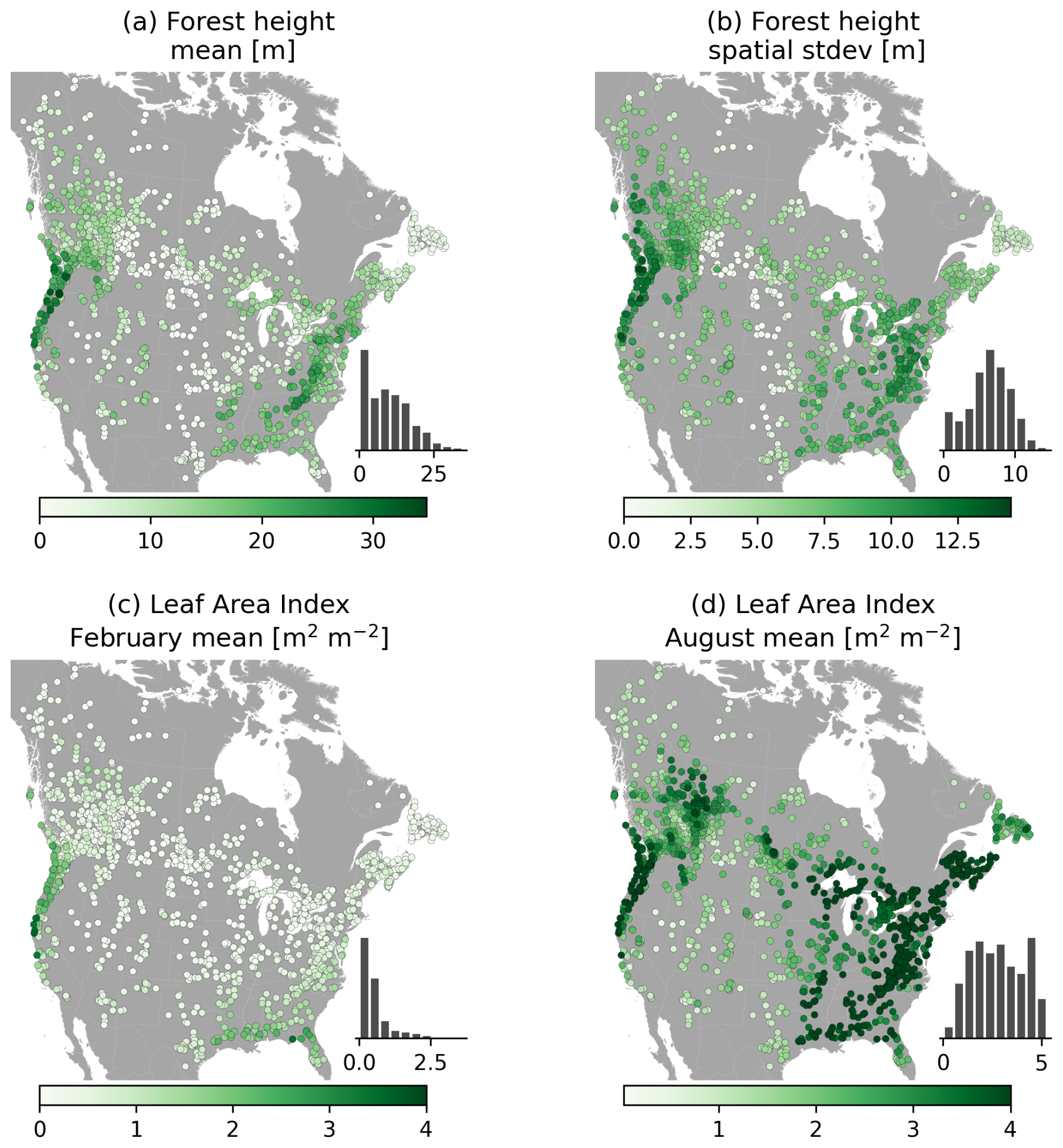
Figure 7 Selection of vegetation attributes. (a, b) The mean and standard deviation of forest height in each basin are derived from the Global Land Cover and Land Use Change dataset and are shown here for the year 2020. (c, d) Leaf area index values are derived from the MODIS MCD15A2H.061 dataset and are shown here as long-term averages values for February and August.

3.4 Subsurface attributes

Attributes describing each catchment's subsurface characteristics are listed in Tables A8 and A9. Figure 8a and b show SoilGrids estimated sand content in the top layer of each catchment and the within-catchment standard deviation of this estimate, respectively. Sand content is often combined with clay and silt content estimates to derive soil parameters used in models, such as porosity and drainage rates. Within-catchment standard deviations tend to be around 20 % of the estimated sand content, suggesting that within-catchment drainage properties can vary considerably. For a given depth, the SoilGrids property of interest (here, sand content) is estimated with a lower bound (Q0.05), median (Q0.50) and mean value, and upper bound (Q0.95). The prediction uncertainty is then calculated as the ratio of the 90 % prediction interval (Q0.95–Q0.05) and the median (Q0.50). Prediction uncertainty (Fig. 8c) adds more variability to the sand content estimates, although this is somewhat modest compared to the within-basin variability of sand content estimates (Fig. 8b). The spatial standard deviation of the uncertainty estimates is even smaller: a couple of percentage point difference at most (Fig. 8d). This suggests that the prediction intervals for sand content, in this layer at least, are relatively narrow. The main variability occurs in each catchment, further emphasizing that going beyond lumped representations of hydrologic behaviour may be useful. This is further supported by Fig. 8e and f, showing the estimated thickness of sedimentary deposits and their spatial standard deviation, respectively. There are clear large-scale patterns of the catchment mean values, where plains and flat areas show the thickest layers. Within-catchment variability is particularly large in catchments with sharp topographic relief (compare Fig. 6b), showing the difference in soil structure between high steep mountains and valley bottoms. However, soil properties are difficult to measure and as a result can be highly uncertain. We urge readers to consult the publications describing these datasets to understand how these values were derived and how they may feed into new work.

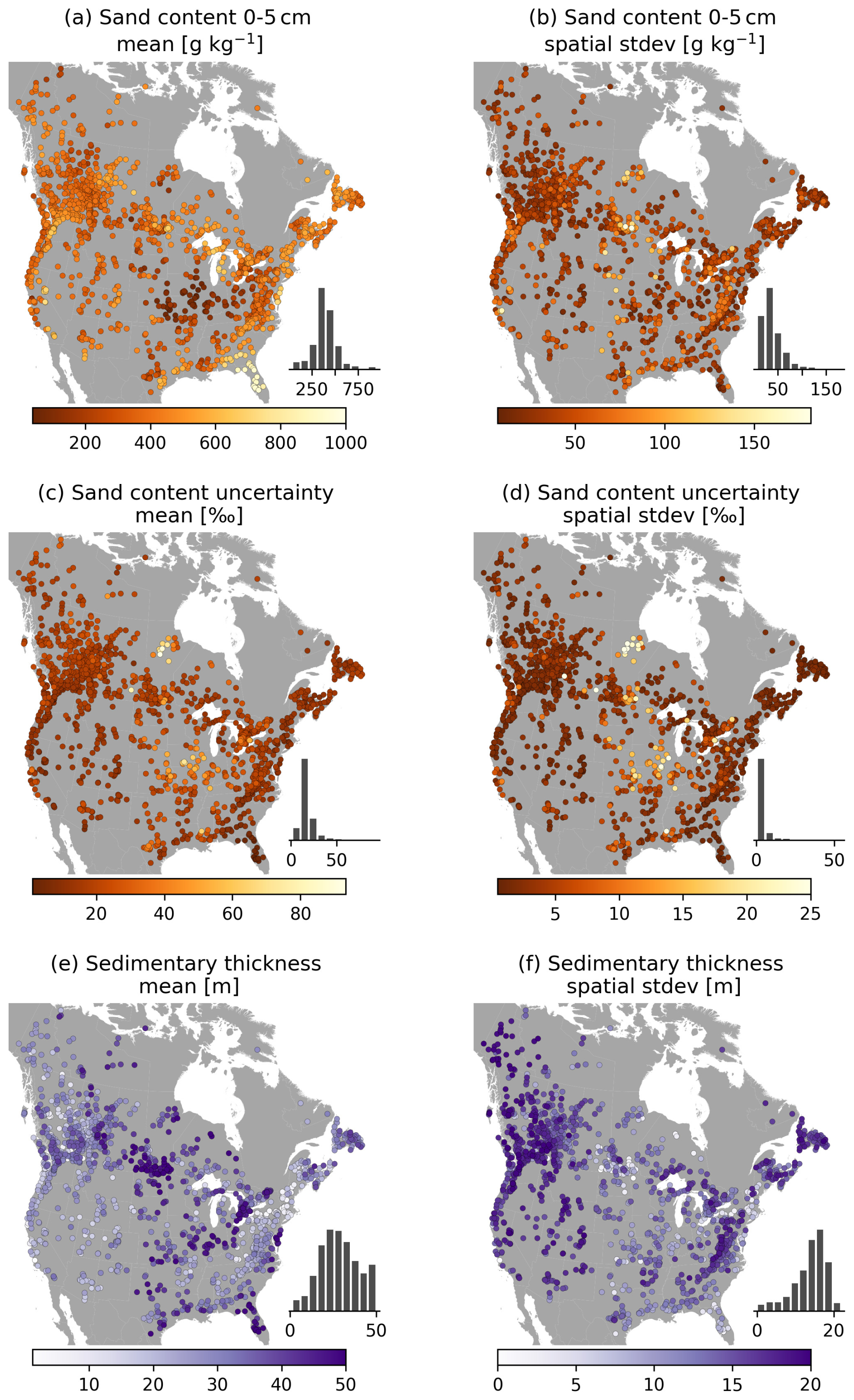
Figure 8 Selection of subsurface attributes. (a–d) Properties derived from the SoilGrids 2.0 dataset through spatial averaging for each catchment. (a, b) Mean and spatial standard deviation of sand content in the top SoilGrids layer. (c, d) Mean and spatial standard deviation of sand content uncertainty, defined as the ratio between the 90th-percentile prediction interval and the median prediction $\left(\frac{\text{Q95}-\text{Q05}}{\text{Q50}}\right)$. (e, f) Mean and spatial standard deviation of sedimentary deposit thickness estimates in the Pelletier dataset.

3.5 Hydrologic signatures

Statistics that describe flow regimes, commonly called signatures, are an active area of research (e.g. McMillan, 2021). As an initial start, we provide the same signatures as provided in the original CAMELS dataset and expand upon these in a number of ways: (1) in addition to mean values, we provide standard deviations when applicable; (2) we provide monthly runoff signatures to complement the monthly climate attributes; and (3) we expand the no-, low- and high-flow duration signatures to include median, skewness and kurtosis values. For the signatures in Table A10, we calculate the signature per year of data first and then find the mean and standard deviation (if applicable) across years. For the statistics for the no-, low- and high-flow periods (Table A11), we instead use all years together and calculate the statistics from this single longer time series.

A subset of these hydrologic signatures is shown in Fig. 9. As expected, the signatures show strong relations to the climate attributes in Fig. 5a and b. Mean discharge (Fig. 9a) is particularly high in non-arid areas, and the standard deviation of annual mean discharge (Fig. 9b) suggests strong intra-annual variability in the observed runoff at most gauges. The influence of snow processes can clearly be seen in the differences between the May and December mean runoff values (Fig. 9c, d). Low-flow duration (Fig. 9e; defined as days where discharge is below 20 % of the mean discharge for the basin) emphasizes the seasonality in runoff patterns in most of these basins. However, these mean values are likely not particularly representative of the duration of low-runoff events. In the majority of basins, the distributions of low-flow durations (as well as no-flow and high-flow durations; not shown for brevity) are positively skewed (Fig. 9f). This indicates that these distributions have heavy tails and that the mean values may be heavily biased by a relatively small number of events. In many basins, the median duration may provide a more representative value of the typical no-, low- and high-flow durations. Almost all recent large-sample datasets provide a mean duration of no-, low- and high-flow events, but the skewness and kurtosis of the underlying distributions are typically not accounted for. This leads to an overestimation of the typical duration of these events and may hinder classification efforts. We strongly suggest that the shape of the duration distributions is accounted for in future work.

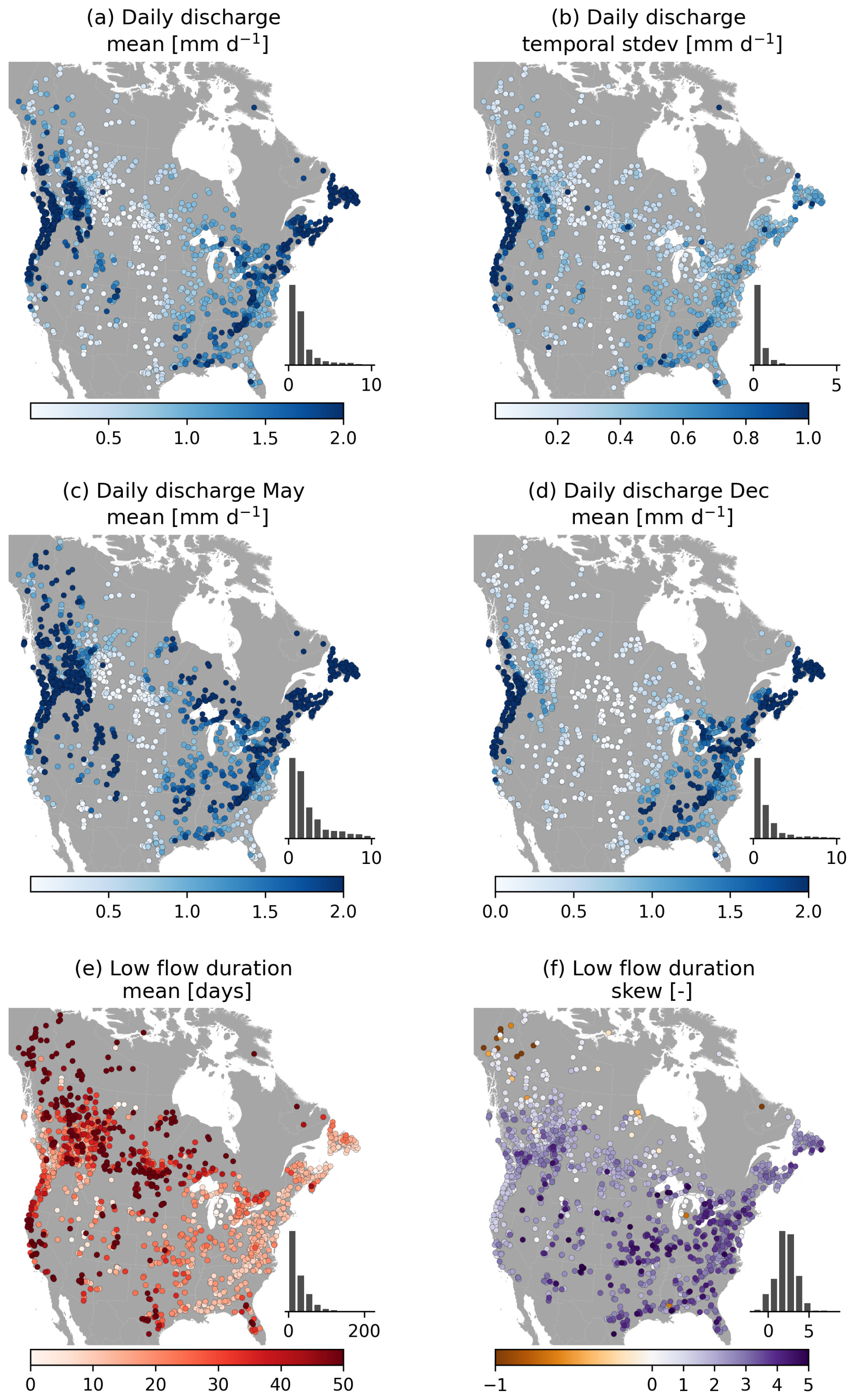
Figure 9 Selection of hydrologic signatures, derived from time series of daily data provided by USGS and WSC.

4 Discussion

4.1 Recommendations for data providers

4.1.1 Dimension boundary information in publicly available data

In Sect. 2.3 and 2.4, we describe the processing of streamflow observations and meteorological data, respectively. One challenge here is determining the representativeness (or validity) of data values in time and space. Data can be instantaneous (i.e. valid at a specific point in time) or time averaged (i.e. valid over a specific time window), and treating one as the other leads to incorrect estimates of fluxes and thus state changes in the system (see also the derivation of hourly flow values in Sect. S1 in the Supplement). The same concern applies to space: values may be representative for a specific point or averaged over a given region. Accounting for these differences is not always straightforward, in particular because information about the spatial and temporal validity of publicly available data is not always easily available and may require informal inquiries to obtain. This hampers the correct application and interpretation of data and can lead to easily preventable biases in analyses and modelling efforts.

A simple solution is provided by the NetCDF Climate and Forecast (CF) metadata conventions (see Sect. 7 in Eaton et al., 2023). These conventions describe the specification of bounds for coordinate variables (i.e. dimensions such as latitude, longitude and time) that indicate between which coordinate values a given data value is considered valid. Specific examples for spatial gridded data can be found in Sect. 7.1 in Eaton et al. (2023), and time bounds are discussed in Example 7.5 and 7.6. The CF conventions are designed for NetCDF files, but the principle of specifying dimension bounds in time and space between which data values are valid is widely applicable. We strongly recommend that including these bounds as part of data distributions becomes standard practice.

4.1.2 Sub-daily flow data derivations

Process-based models can be useful for long-term water assessments, provided that they are parameterized well and that the theoretical underpinnings of the model are valid (e.g. Kirchner, 2006; Clark et al., 2016). In the case of process-based models, assessing a model's physical realism requires observations at a sub-daily resolution. In CAMELS-SPAT, we therefore construct hourly streamflow series from time series of instantaneous streamflow observations that are publicly available. However, the phrase “streamflow observations” (although common) is somewhat misleading: in almost all cases, the observations are of water levels, and streamflow values are estimated for a given water level with rating curves. Especially at high observation frequencies, these water levels may be subject to random fluctuations unrelated to streamflow magnitude (e.g. due to wind or small eddies), which will translate into streamflow estimates affected by this noise. A cleaner approach would be to find the average hourly water level and estimate the average hourly flow from this through the station's rating curve. Development and maintenance of rating curves is complex, however, and rating curves tend to change through time (see for example the description of WSC's procedures in  Gharari et al., 2024). Computing robust sub-daily streamflow estimates will be easier at the institutional level (not least because it requires access to the rating curves), and we express the hope that this may become standard practice.

4.2 Guidelines for practical use

Here, we outline various considerations that may be useful to readers. Our goal with these is to set expectations for dataset use and to highlight potential pitfalls that may not be immediately obvious.

4.2.1 Summary sheets of basin conditions

Following Delaigue et al. (2024), we created summary sheets of the conditions in each basin. These summaries are intended to aid quick assessments of each basin and cover the following elements: (1) identifier, location and long-term statistics (i.e. mean precipitation, streamflow, temperature, potential evapotranspiration, aridity and runoff ratio); (2) various graphics showing more detailed statistics (e.g. year-to-year variability in streamflow, mean monthly temperature ranges and elevation distribution); and (3) various maps showing the spatial variability of various key attributes (i.e. elevation, land cover, agriculture presence, forest height, soil class and soil depth). An example can be found in the Supplement, Sect. S5. The full collection of summary sheets is available on the data repository. Section S5 also contains an example that highlights the need to apply a basin mask when working with the GeoTIFF maps provided as part of the CAMELS-SPAT data: in certain cases, pixel values outside the basin boundaries will contain values that are within the valid data range (for example, forest height values outside the basin are set to 0 m). Applying a basin mask ensures that only values within the basin boundaries are used in any analysis that relies on the GeoTIFF files.

4.2.2 Selection of time periods

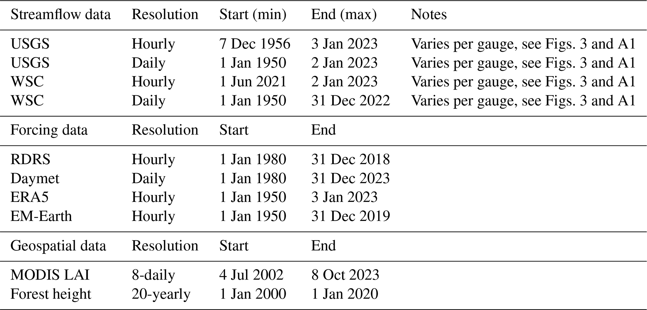
Our aim with CAMELS-SPAT is to facilitate a wide range of studies, and we have therefore provided as much data for each gauge as seemed feasible. In particular, this meant that we only excluded station observations before 1950, because none of the forcing datasets covers this period, and we also accepted the fact that not all forcing products are available for the full period for a given gauge. For different purposes, it will thus be necessary to subset the data we provide to shorter time periods. Table 4 provides an overview of the time periods covered by the various data products that may assist in selecting appropriate periods for specific studies.

Table 4 Time periods covered by the different datasets included in CAMELS-SPAT. Geospatial data not listed are static products that have no time dimension.

4.2.3 Utilization of streamflow data quality flags

We retained streamflow observation quality flags provided by the USGS and WSC during processing and stored these in the same NetCDF files as the streamflow observations themselves. These flags indicate conditions affecting the streamflow measurement, such as the presence of river ice, backwater effects, water levels below sensor level or equipment malfunction. These conditions suggest that streamflow data at these time steps may be inaccurate (even if the discharge data at such time steps are corrected by the data provider, large uncertainties may remain; see Gharari et al., 2024), and this may affect analyses that use these data. For example, it is known that differences between observed and simulated streamflow at individual time steps may have disproportionate effects on aggregated efficiency scores that are used in modelling (e.g. Newman et al., 2015; Clark et al., 2021), and, if one tries to match incorrect “observations”, this may negatively impact the quality of the resulting model configuration. Excluding streamflow observations from efficiency score calculations based on data quality flags is a possible way to limit the impacts of potentially erroneous streamflow values.

4.2.4 Spatial validity of meteorological forcing data

CAMELS-SPAT contains meteorological data from four different datasets at their original gridded resolution, as well as averaged at the basin and sub-basin level. During this averaging process, we assumed that values provided at specific coordinates are valid for a grid cell around this point. This is a simplistic approach, but it is somewhat difficult to justify more elaborate assumptions (such as some form of interpolation), because in reality the change of meteorological variables in space would be dependent on local topography at scales smaller than the typical forcing data grid cell. Interpolation methods may yield more realistic sub-basin and basin-averaged values, but it is beyond the scope of this paper to investigate these.

4.2.5 Combing soil depth and soil property estimates

CAMELS-SPAT contains both estimates of soil depth (derived from the Pelletier dataset; Pelletier et al., 2016a, b) and soil properties (derived from the SoilGrids 2.0 dataset; Poggio et al., 2021). Because the SoilGrids data assume a uniform depth of 2.0 m everywhere, soil properties will thus be unknown for actual soil depths greater than 2 m or incorrectly provided for actual soil depths less than 2 m. For estimated depths below 2 m, an appropriate approach may be to only use the SoilGrids layers that correspond to the estimated soil depth. For estimated soil depths greater than 2 m, recommendations are more difficult to provide. Appropriate approaches may be the derivation of pedotransfer functions or reliance on simple assumptions that extend the available layer information to deeper depths.

4.2.6 Modelling the Prairie Pothole Region

Model performance across the US is known to change regionally, where model performance is at its worst in the drier central regions (e.g. Newman et al., 2015; Towler et al., 2023). In CAMELS-SPAT, we compound this problem by including basins from the so-called Prairie Pothole Region. This area covers parts of southern Alberta, Saskatchewan, Manitoba, North Dakota, South Dakota, Minnesota and Iowa and is colloquially known as the “graveyard of hydrological models” (e.g. Muhammad et al., 2019; Budhathoki et al., 2020; Ahmed et al., 2023). The landscape in the Prairie Pothole Region is relatively young on a geological time scale, and large parts of it have not yet eroded into traditional river networks. Surface depressions are common and typically not connected to the stream network, except through very slow groundwater drainage and the occasional fill-and-spill event (Hayashi et al., 2016; Clark and Shook, 2022). In the basins we provide as part of the CAMELS-SPAT data, all sub-basins are connected to the stream network. However, surface depressions below the resolution of the MERIT DEM are common and will affect hydrologic behaviour in these (sub-)basins. We recommend that users account for these potholes in their analyses and modelling efforts, possibly through the use of stand-alone models or post-processing tools (e.g. Clark and Shook, 2022), by adapting existing models with an appropriate landscape module (e.g. Ahmed et al., 2023), or by adjusting their expectations of model performance accordingly.

4.2.7 Selection and extension of catchment attributes

We derived various catchment attributes for the basins in CAMELS-SPAT for ease of use and comparison with existing datasets. However, the number of attributes included in CAMELS-SPAT is rather high, and we encourage others to make a careful selection of which attributes to use in their own work. Attribute values can show considerable correlations, and using a greater number of attributes will not necessarily add an equal amount of new information. Higher numbers of attributes will, however, increase computation and analysis times for applications such as regionalization, clustering and data-driven modelling. A more fruitful approach likely relies on defining hypotheses that can be tested with catchment attributes and deliberately selecting the right attributes for these tests. If our initial attribute calculations do not offer the right choices, new attributes can easily be derived from the data products included in CAMELS-SPAT. We refer the reader to Tarasova et al. (2024) for a deeper discussion and recommendations on the use of catchment descriptors. We particularly encourage investigations that evaluate the usefulness of our provided attributes for catchment characterization purposes, in line with those recommendations.

4.2.8 Potential evapotranspiration estimates

In order to facilitate a wide range of modelling studies, CAMELS-SPAT contains a variety of estimates of potential evapotranspiration (PET). These can be used as inputs to certain types of models and to calculate certain climatic attributes such as a basin's aridity. However, there are multiple ways to estimate PET depending on data availability and purpose (McMahon et al., 2013), and this results in a certain amount of uncertainty in these PET estimates and any values derived from them. Here we provide a brief overview of the various PET estimates available in CAMELS-SPAT, along with a brief assessment that may help users to decide which data to use. Table 5 summarizes this overview.

CAMELS-SPAT contains time series of PET (variable name mper) that are provided as an extra output of the ERA5 modelling chain (although note that this variable is not used directly in the production of ERA5 or the generation of forecasts). However, these values are known to be locally deficient in regions without low vegetation (see https://confluence.ecmwf.int/display/CKB/ERA5%3A+data+documentation#ERA5:datadocumentation-Knownissues, last access: 9 May 2025, Sect. “Known Issues”, bullet point 15). This is also reported by Clerc-Schwarzenbach et al. (2024), who point out that PET data obtained from ERA5-Land must be treated carefully and may include unrealistic values. Section S4 in the Supplement contains a preliminary analysis that identifies where these issues are present in the mper data included in CAMELS-SPAT. We have kept the ERA5 PET estimates as a reference for users who wish to investigate this further but urge caution about their use.

CAMELS-SPAT also contains time series of PET estimates obtained with the Penman–Monteith method and hourly RDRS data, as well as time series of PET estimates obtained with the Priestley–Taylor method and daily Daymet data. Finally, we included spatial PET estimates using the temperature-based method in Oudin et al. (2005), applied to monthly averaged WorldClim data. Equations for all three approaches can be found in Sect. S2.5 in the Supplement. We compared these to the PET estimates from Singer et al. (2021) and their overview of mean annual PET estimates from various products in their Fig. 1 and Table 2. Preliminary analysis (see Sect. S4 in the Supplement) suggests that our PET estimates from RDRS, Daymet and WorldClim all exhibit similar spatial patterns to the five datasets shown in Singer et al. (2021). Visual comparison also suggests that there is some spread in the magnitude of our estimates. Monthly estimates based on WorldClim data are low compared to the other methods and data sources and comparable to those in GLEAM. Daily estimates based on Daymet data are close to the middle of the range of estimates. Hourly estimates based RDRS data are within the ranges of estimates provided by the other methods and datasets, although somewhat high compared to most other products.

Due to the lack of uniformity in PET definitions and calculation methods (e.g. McMahon et al., 2013), it is difficult to say which estimates are the most accurate. For time series, any expected systematic biases could be corrected before using the time series as a model input. Derived statistics with clear physical interpretations, such as aridity, are more difficult. A basin may be classified as either water limited or energy limited solely as a consequence of the data and PET estimation method used, and this may hinder classification and interpretation efforts. Possible ways around this may involve the use of multiple estimates of PET-related attributes. We thus recommend caution when selecting and interpreting any PET estimates for further use.

Oudin et al. (2005)

Table 5 Overview of PET estimates in CAMELS-SPAT, how they are used in CAMELS-SPAT and a summary of how these values compare to each other as well as the estimates from five other PET estimates listed in Singer et al. (2021).

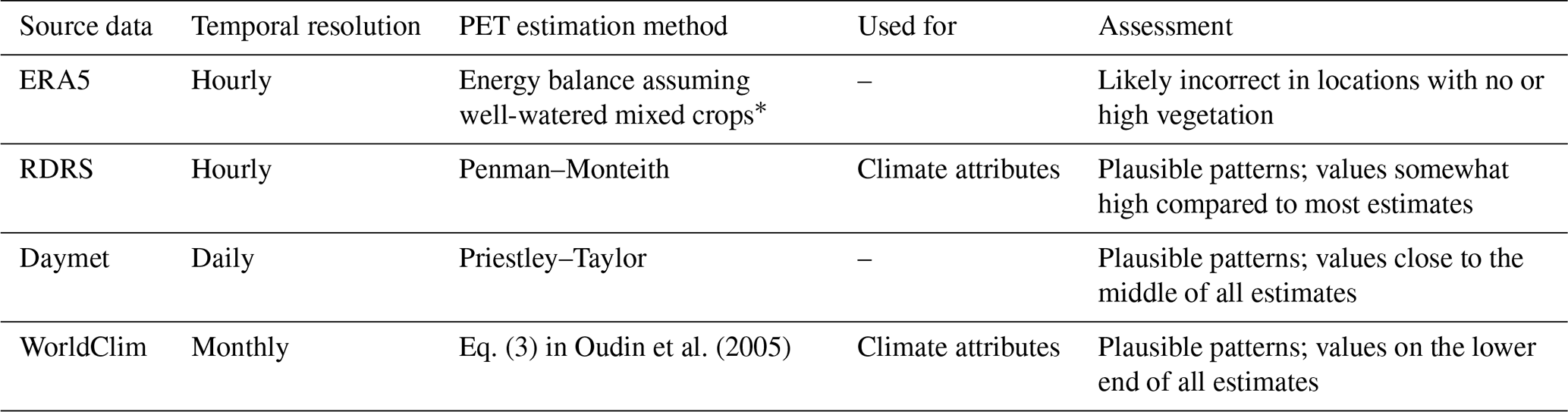
^∗ PET variable mper is derived from variable pev. For more details about the calculation of pev, see https://codes.ecmwf.int/grib/param-db/228251 (last access: 9 May 2025).

4.3 Potential improvements

CAMELS-SPAT represents a substantial data-processing effort, but further enhancements are possible. We briefly list these here. First, approximately 15 % of our basin outlines have been assigned confidence ratings of medium or low. Future efforts can focus on refining these outlines through further manual intervention, higher resolution DEMs or both. Second, we necessarily needed to limit the extent of our geographical domain, and this means that there is a limit to the different types of landscapes our dataset covers. However, apart from Daymet and RDRS, all datasets used here have global coverage. Combination with local streamflow observations, and possibly high-quality local datasets, should allow for an extension of the dataset to other regions. The code available on our GitHub repository could provide a starting point for such efforts. Third, extending the dataset to include observations or estimates of variables of interest other than streamflow would help with multi-variate analysis and model evaluation. Examples include satellite observations of snow cover or estimates of evaporation fluxes or water storage in the soil.

4.4 Dataset structure and size

For convenience, we divided the collection of 1426 CAMELS-SPAT gauges into various subsets. At the highest level, we structured the dataset with different folders for attributes, forcing data, geospatial data, observations and shapefiles. At the next level, we divided the dataset into three categories of headwater and meso-scale and macro-scale basins. Headwater basins are defined as catchments with only a single sub-basin in our delineation (note that for these basins, the lumped and distributed cases are identical). Meso-scale basins are basins that are not headwaters and below a total area of 10³ km², and macro-scale basins are those with areas between 10³ and 10⁴ km². Headwater basins account for 304 out of 1426 total (mean area of approximately 60 km²), 727 basins fall into our meso-scale category (mean area ≈400 km², with on average nine sub-basins) and the remaining 446 basins are macro-scale basins (mean area ≈ 3000 km², on average 66 sub-basins). From here we divided the dataset into further subfolders when convenient.

The total size of the CAMELS-SPAT data is approximately 5.5 TB. Almost all of this is forcing data (5.4 TB) and specifically the gridded variants of the forcing data (4.3 TB). Basin-averaged data (summed for all four forcing datasets) sum up to 85 GB, while distributed forcing data (i.e. averaged at the sub-basin level) sum up to not quite 1.2 TB. A full overview of the size of various components of the dataset can be found on the data repository. This overview, combined with the overall folder structure, should allow users to fine-tune their downloads easily. Further instructions to include or exclude components from the download can be found on the data repository.

5 Conclusions

This paper describes the development of the CAMELS-SPAT dataset. Our goal is to enable a wide range of hydrologic studies, with a particular focus on hydrologic modelling, by performing a wide range of data-processing steps and sharing both the code and outcomes of these. We extend the original CAMELS data (Newman et al., 2015; Addor et al., 2017a) in five ways to achieve this goal. First, we extend the geographical domain of the dataset beyond the contiguous US by including Canadian basins. Second, we provide meteorological data specifically aimed at spatially distributed physics-based hydrologic models, in addition to the inputs needed to run lumped conceptual models. Third, we provide streamflow data at both daily and hourly time steps for each basin. Fourth, we provide maps of multiple geospatial datasets for each basin, rather than only a selection of summary statistics derived from these maps. Fifth, we provide a variety of catchment attributes intended to describe the spatial and temporal range of our attributes, in addition to the more commonly provided mean attribute values.

CAMELS-SPAT thus consists of meteorological data, streamflow observations and geospatial data for 1426 basins across the US and Canada. The meteorological data include a number of variables typically associated with process-based models, as well as potential evapotranspiration estimates that can be used with the more conceptual model types, at hourly time steps (daily for the Daymet data). These forcing data are provided in a gridded format at their original resolution, as well as spatially averaged at the sub-basin and basin level. Streamflow observations are provided at daily time steps and complemented with hourly observations when these are available. Geospatial data, covering vegetation, land use, topography, soil and geology, are provided as georeferenced maps for each basin from which model inputs or summary statistics that go beyond our provided attributes can easily be derived. Finally, the information for each gauge (streamflow, meteorological, geospatial data) is summarized in an extensive number of catchment attributes, at both the basin and sub-basin level.

In developing CAMELS-SPAT, we focused on providing the necessary data for a wide variety of studies. We envision the data being helpful for studies aimed at improving our understanding of hydrologic processes and our ability to model those processes. By removing the need for a considerable amount of cumbersome data processing, we hope CAMELS-SPAT can support a wide range of hydrologic investigations at a fraction of the effort otherwise needed.

The dataset can be accessed through the Federated Research Data Repository (FRDR) at https://doi.org/10.20383/103.01306 (Knoben et al., 2025). When using CAMELS-SPAT, please note the attribution and licence requirements for dataset components outlined in the “Code and data availability” section.

Appendix A: Streamflow data availability

Figure A1 shows streamflow data availability at a more granular level than the aggregated data in Fig. 3.

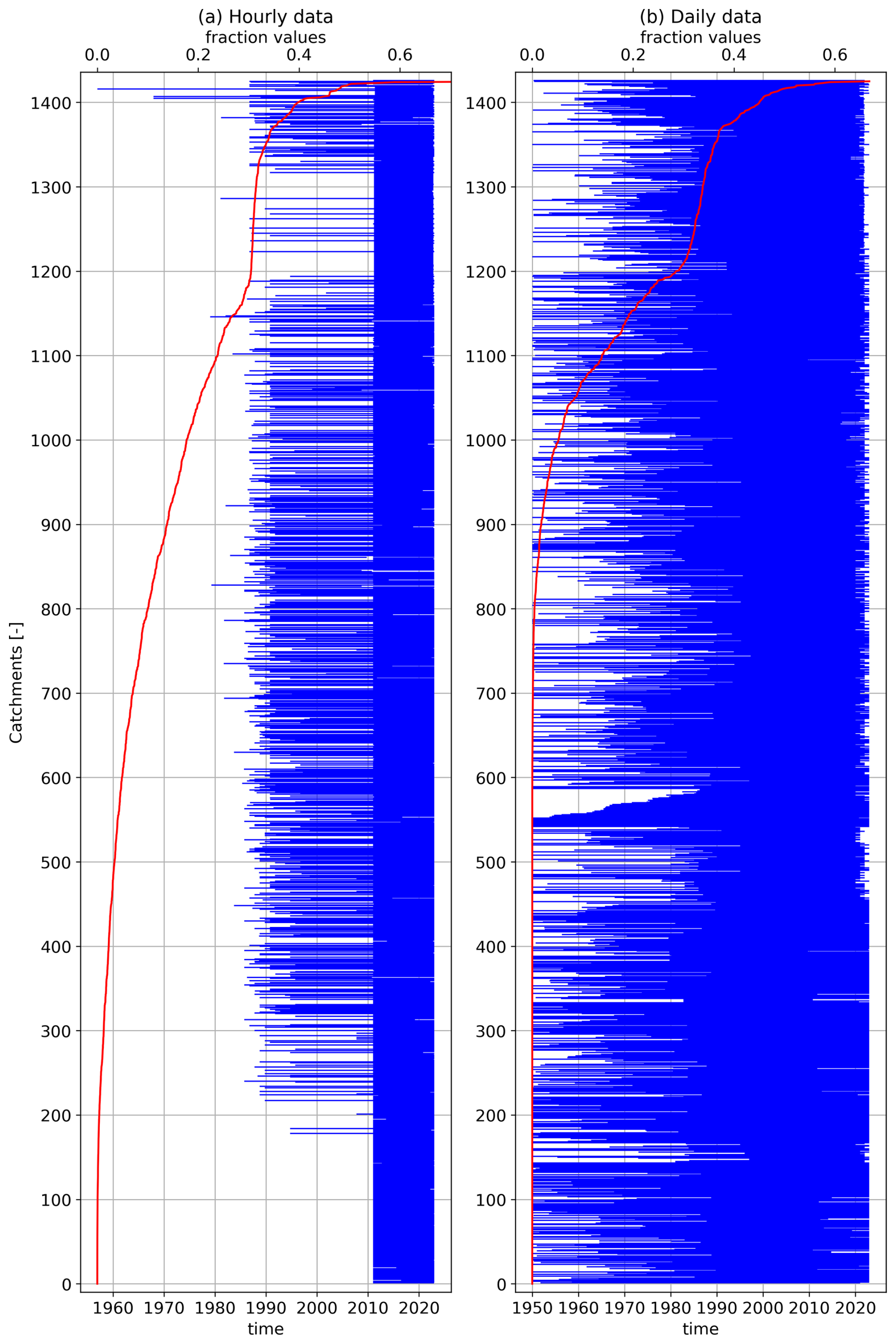
Figure A1 Flow data availability for gauges included in CAMELS-SPAT. The period on the lower x axis refers to the period between the first publicly available flow record for a given station and its last, with this record period given in blue for each gauge. Missing values occur in this record period and are given here in red as a fraction of the total record length on the top x axis.

Table A1 Climate attributes: annual statistics.

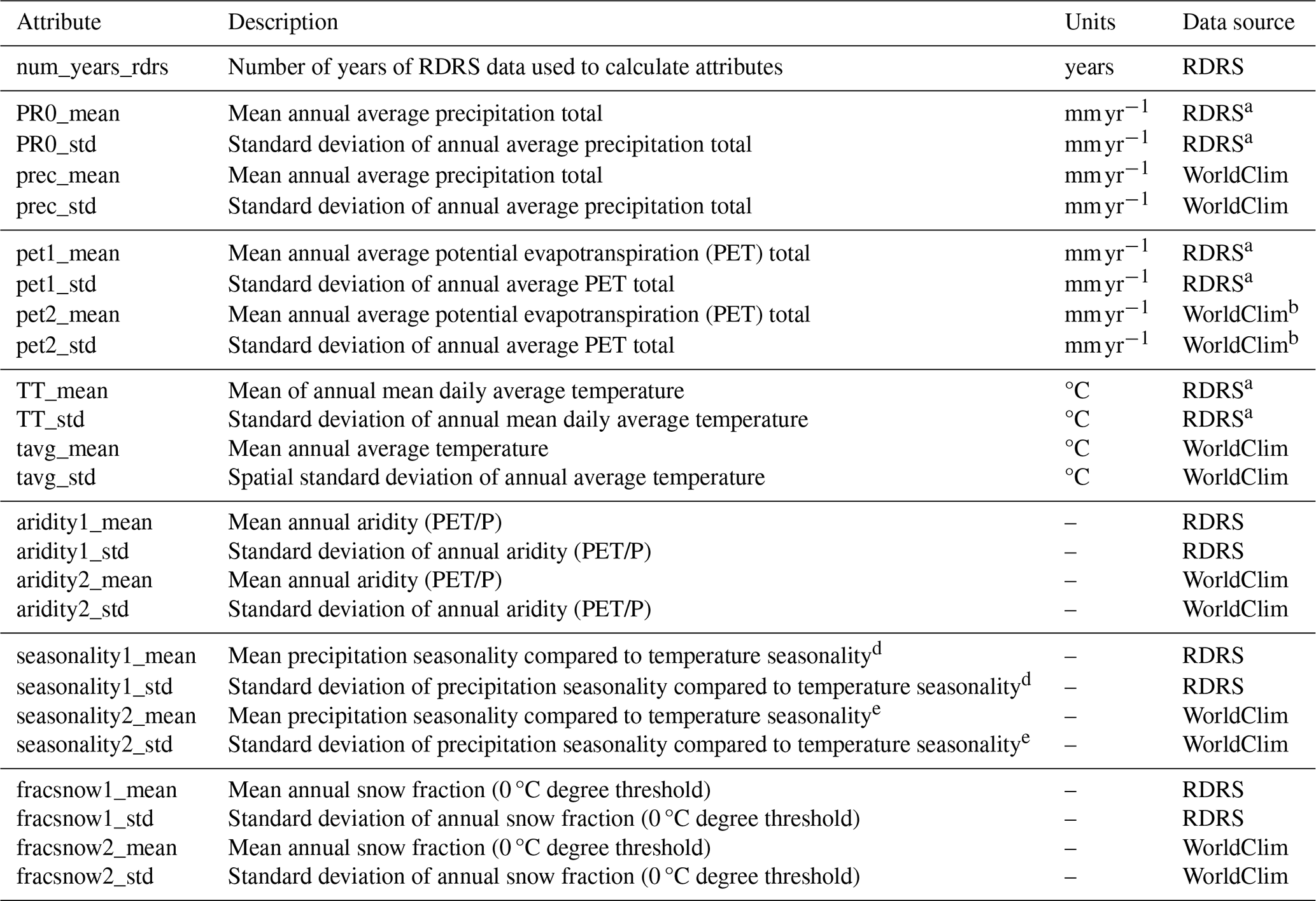
^a For consistency, we converted the RDRS units into those used in WorldClim. ^b Computed using WorldClim's srad and tavg variables and Eq. (3) in Oudin et al. (2005). ^c For consistency, we converted the WorldClim units into those used in RDRS. ^d Calculated using Eq. (14) in Woods (2009) for daily data from individual years, then finding the mean and standard deviation across years. ^e Calculated using Eq. (14) in Woods (2009) using monthly data, i.e. a much coarser temporal resolution than RDRS.

Table A2 Climate attributes – continued: frequency, duration and timing of high and low precipitation and of high and low temperature periods.

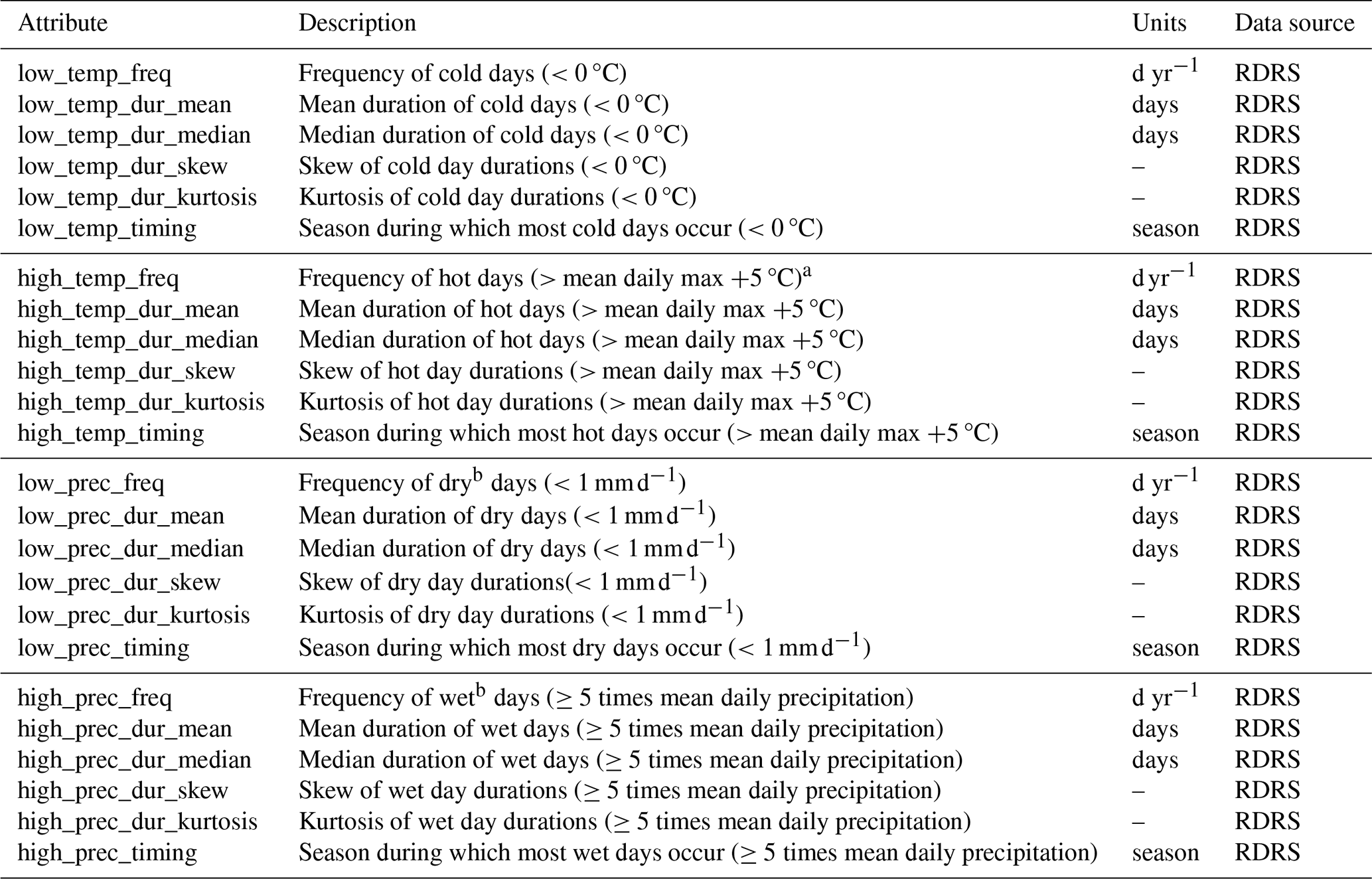
^a Derived from the World Meteorological Organization's definition of heat waves: a 5 d or longer period with maximum daily temperatures 5 °C above the “standard” daily maximum temperature. “Standard” is defined as the mean daily max on each day, using the period 1961–1990 as a base. Here we define a hot day as a day where the maximum temperature is at least 5 °C over the long-term daily maximum temperature. We do not have data for the period 1961–1990 for all basins and therefore use all data available for a given basin to find the long-term daily maximum temperatures. ^b For consistency, we use the same definitions of dry and wet days as used in Addor et al. (2017a).

Table A3 Climate attributes – continued: spatial and temporal variability in climatic conditions. Attributes ending in _{X} are calculated per month, with X ranging from 01 to 12. Statistics derived from RDRS are calculated over time; statistics derived from WorldClim are calculated across space.

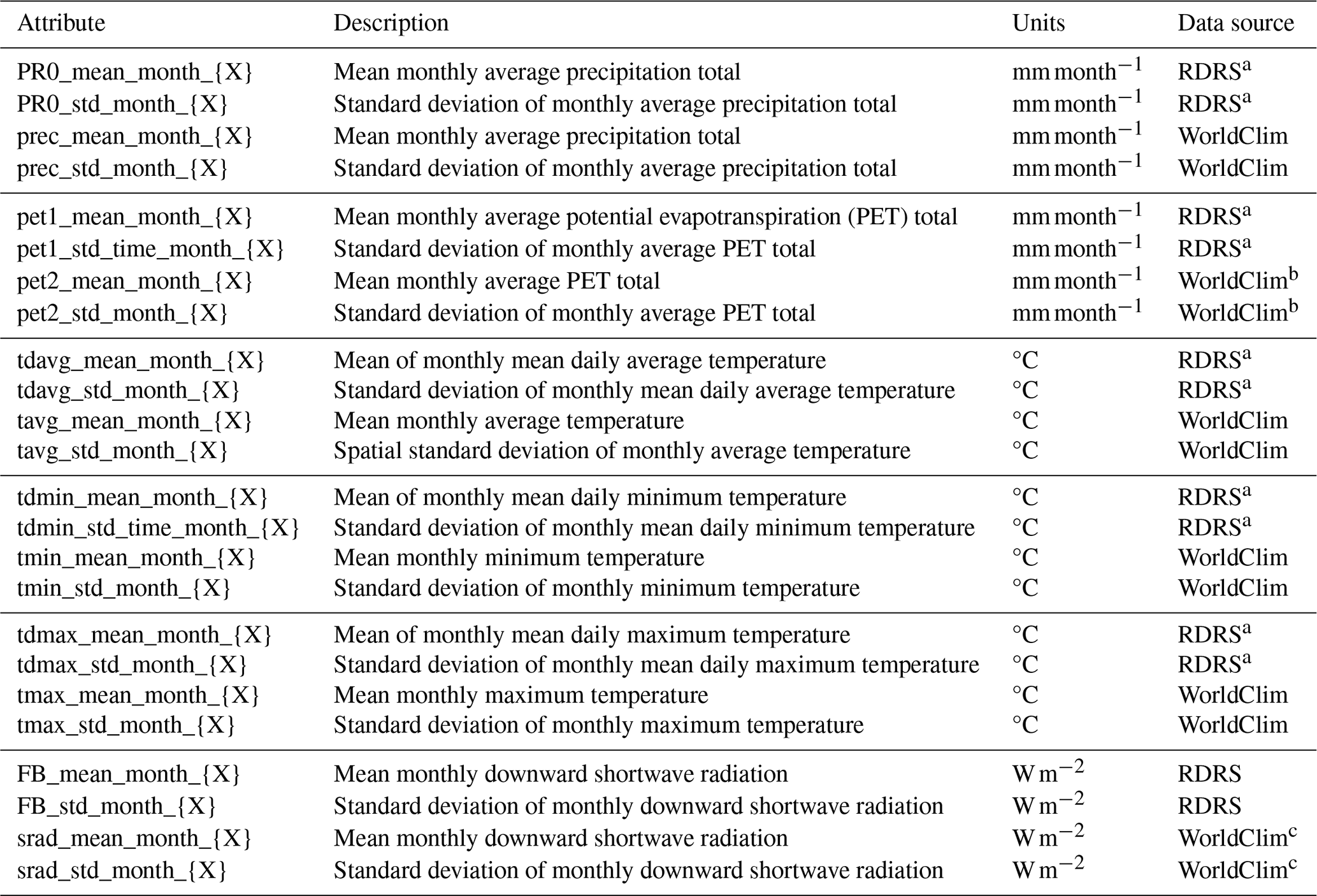
^a For consistency, we converted the RDRS units into those used in WorldClim. ^b Computed using WorldClim's srad and tavg variables and Eq. (3) in Oudin et al. (2005). ^c For consistency, we converted the WorldClim units into those used in RDRS.

Table A4 Climate attributes – continued: spatial and temporal variability in climatic conditions. Attributes ending in _{X} are calculated per month, with X ranging from 01 to 12. Statistics derived from ERA5 are calculated over time; statistics derived from WorldClim are calculated across space.

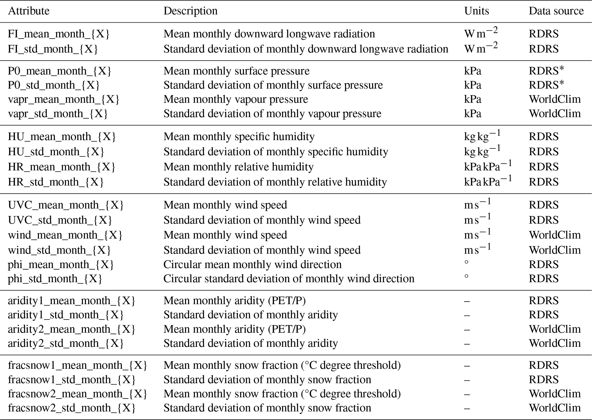
^∗ For consistency, we converted the RDRS units into those used in WorldClim.

Table A5 Topographic attributes.

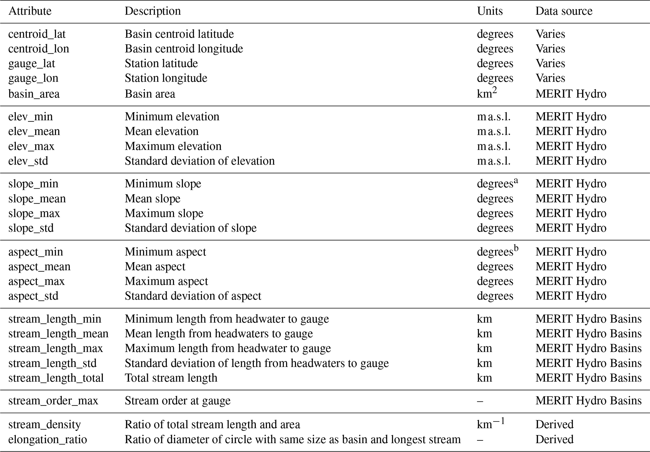
^a Slope angle. ^b Azimuth that slopes are facing, with 0° indicating north-facing slopes, 90° east-facing, 180° south-facing and 270° west-facing.

Table A6 Open water attributes. For basins with no identified open water bodies or reservoirs, these attributes will be 0 and NaN.

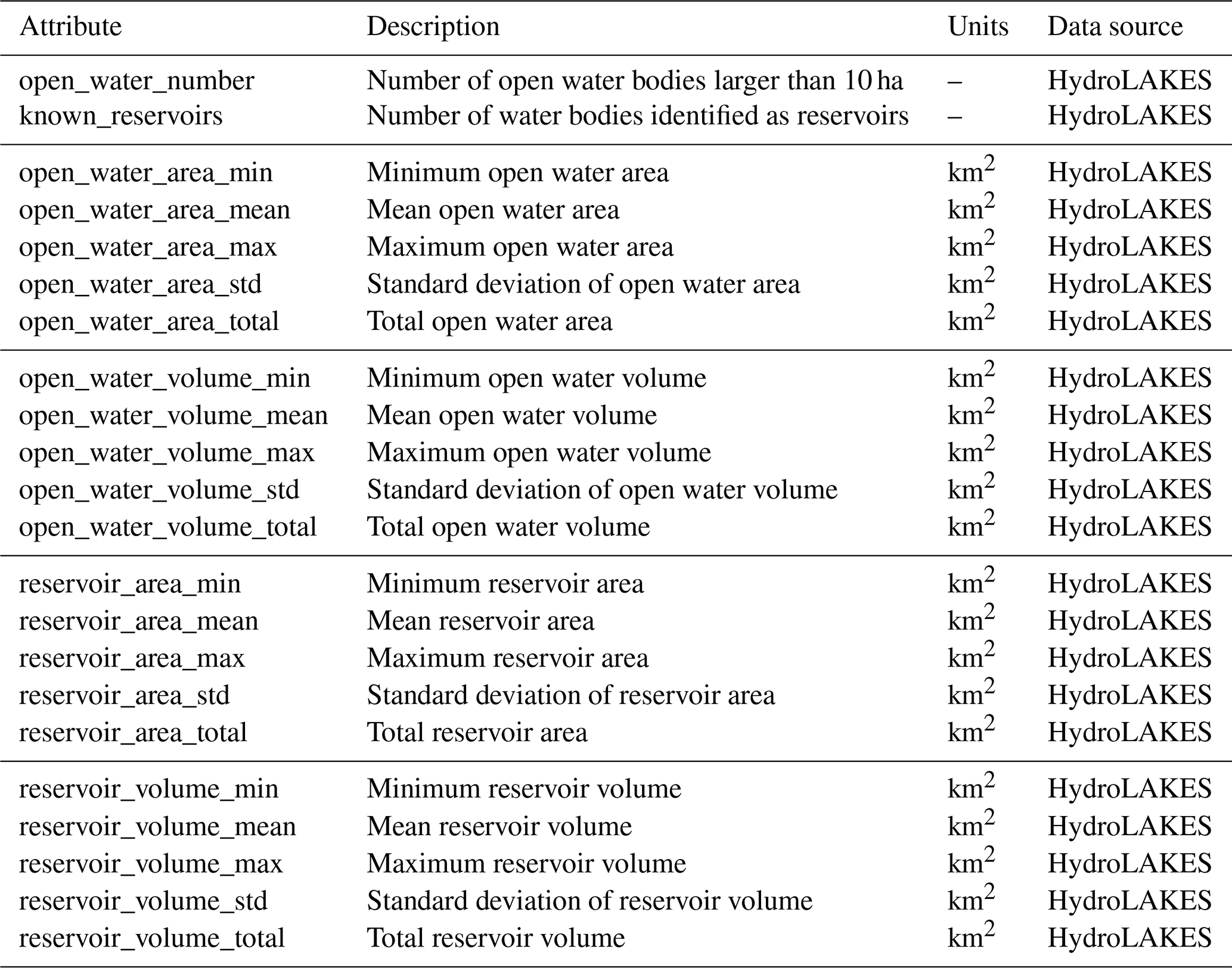
Table A7 Vegetation and land cover attributes. Attributes ending in _{X} are calculated per month, with X ranging from 01 to 12. Attributes ending in _{Y} are calculated for specific years. Attributes ending in _{Z} are categorical attributes, where Z varies between different datasets.

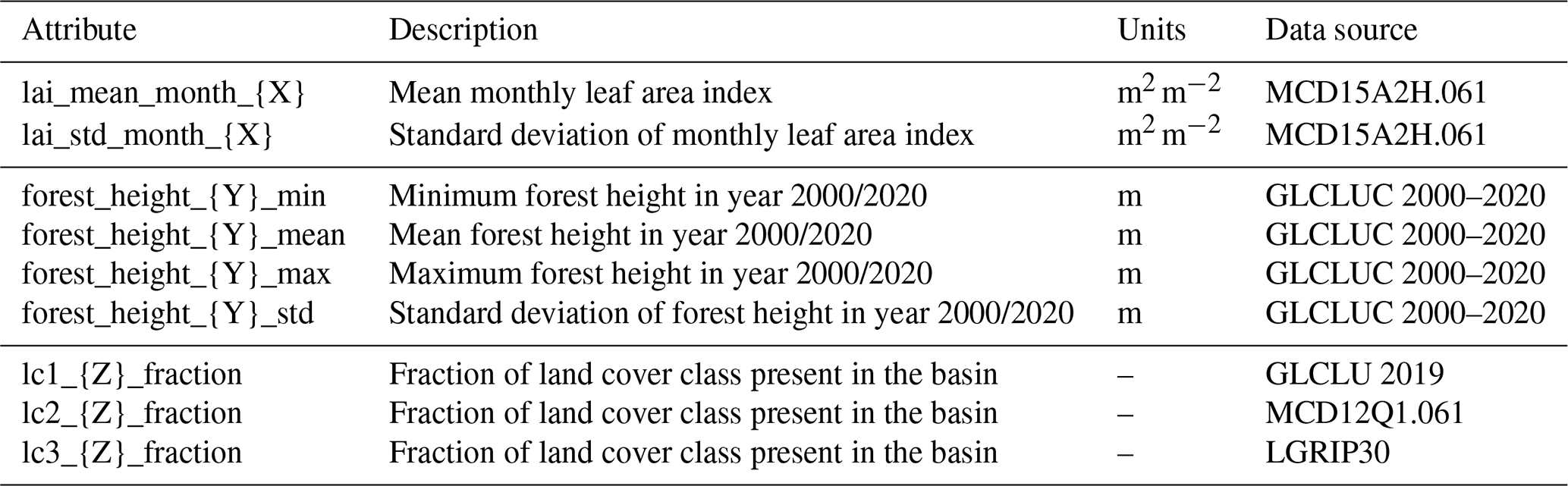
Table A8 Subsurface attributes.

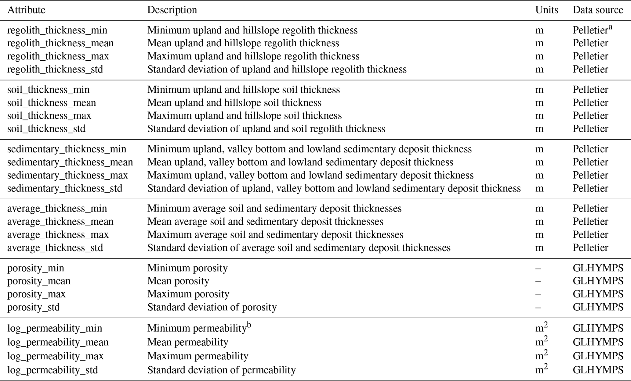
^a For definitions and user notes, see https://daac.ornl.gov/SOILS/guides/Global_Soil_Regolith_Sediment.html (last access: 6 March 2024). ^b Note that permeability k in the GLHYMPS database is given as log 10(k), due to the many decimal places otherwise needed.

Table A9 Subsurface attributes – continued: properties derived from the SoilGrids data. Attributes are provided at six depths {D}: 0–5, 5–15, 15–30, 30–60, 60–100 and 100–200 cm and for the SoilGrids mean (abbreviated in the table as {M}) and uncertainty ({U} in the table) data fields. The mean values may be seen as expected values for a given grid cell, while the uncertainty is defined as the 90 % prediction interval divided by the median value for the cell^a.

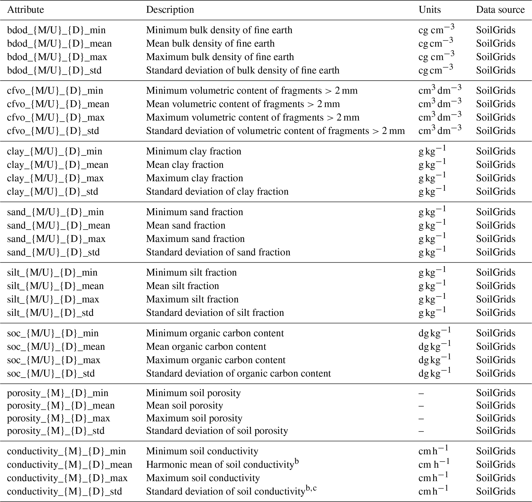
^a See https://www.isric.org/explore/soilgrids/faq-soilgrids (last access: 7 March 2024). ^b Following Addor et al. (2017a). ^c Note that no harmonic equivalent of a standard deviation exists, and this is a regular standard deviation.

Table A10 Hydrologic signatures. Note that streamflow observations have been converted from m³ s⁻¹ to mm d⁻¹ using the basin areas of our newly delineated basin outlines. Please note the uncertainty in these area estimates (Fig. 2). For each signature, we calculated a sequence of yearly values and then found the mean and standard deviation across all years for which data were available.

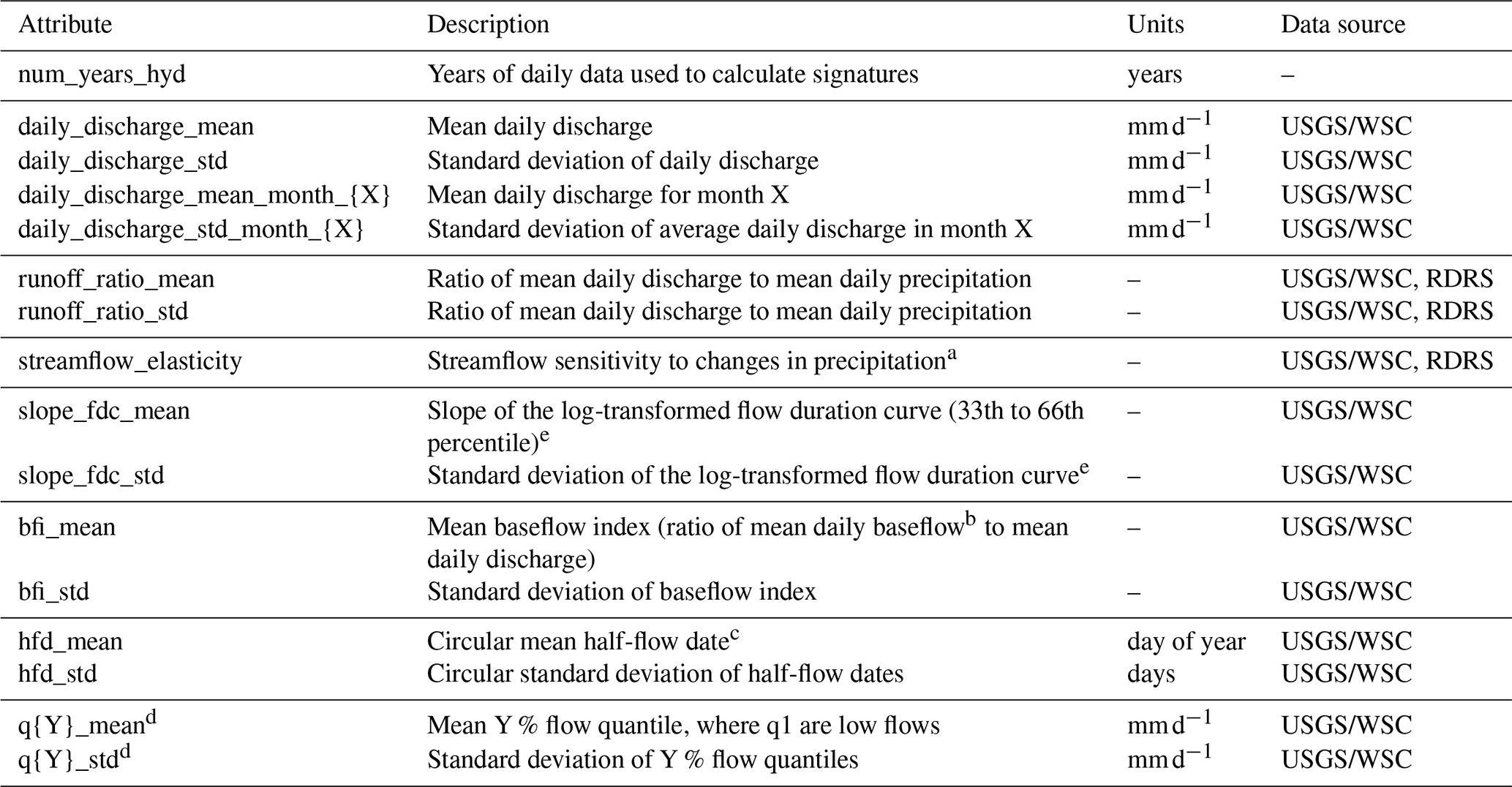
^a Calculated as described in Eq. (7) of Sankarasubramanian et al. (2001), with the modification described in Table 3 in Addor et al. (2017a). ^b Calculated from time series of baseflow derived using the Eckhardt (2005) digital filter method, as recommended and implemented by Xie et al. (2020). ^c Calculated as the day when cumulative flow in a water year passes half the total flow for that water year. ^d Y is one of [0.01, 0.05, 0.10, 0.25, 0.50, 0.75, 0.90. 0.95, 0.99]. ^e In cases with zero flows, 0.1 % of the mean flow is added to prevent issues with calculating the logarithm. Time steps with missing flow observations are removed from the calculation.

Table A11 Hydrologic signatures – continued: frequency, duration and timing of high- and low-flow events.

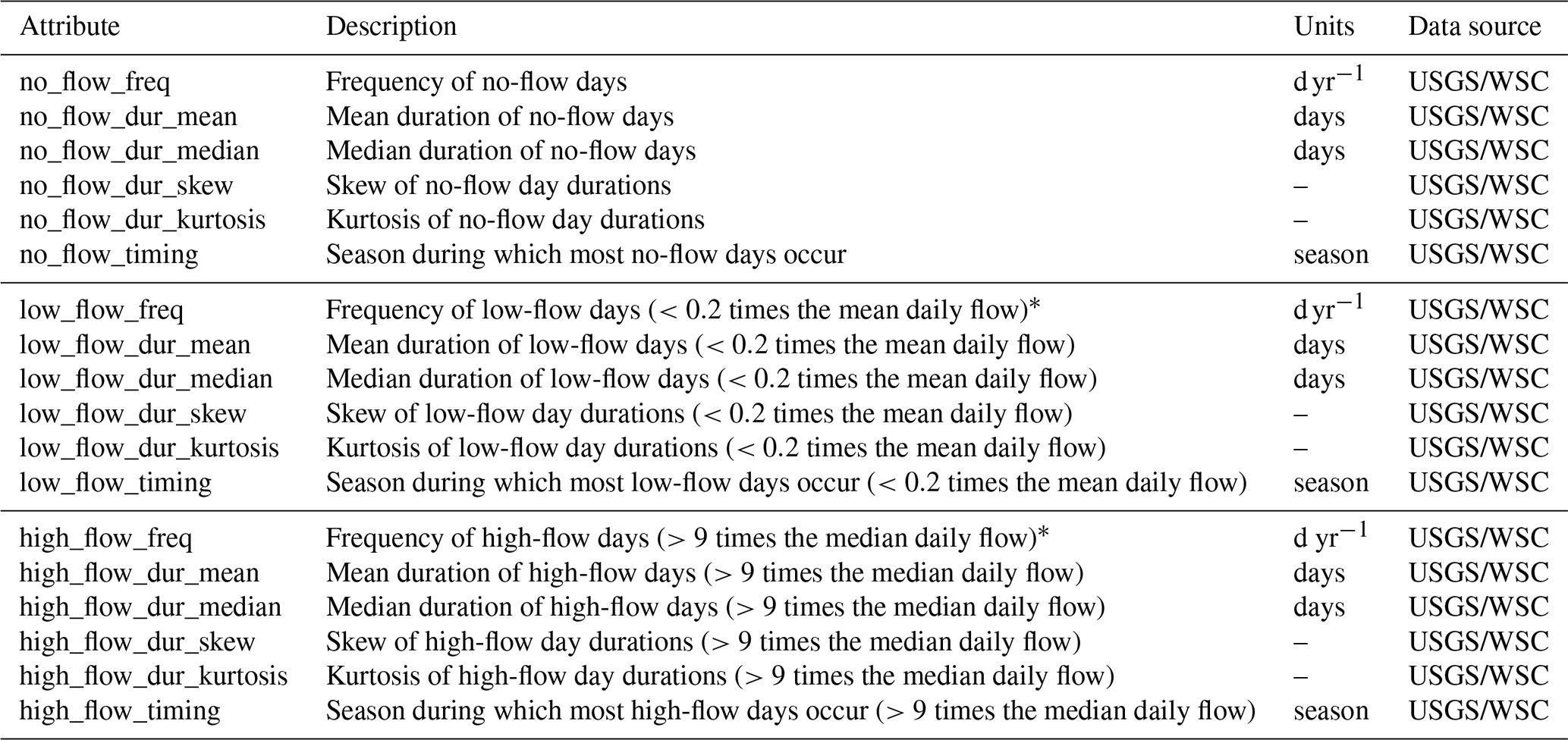
^∗ For consistency, we use the same definitions of dry and wet days as used in Addor et al. (2017a).