Impact of bias adjustment strategy on ensemble projections of hydrological extremes

Hydrological climate change impact studies typically rely on hydrological projections generated by hydrological models driven with bias-adjusted climate simulations. Such hydrological projections are influenced by internal climate variability, which can mask the emergence of robust climate trends. To account for internal variability in climate projections, single-model initial-condition large ensembles (SMILEs) can be employed. SMILEs are generated by running a single global/regional climate model many times with slightly perturbed initial conditions. However, it remains challenging to select an appropriate bias adjustment strategy for SMILEs used in hydrological impact studies because of the relative importance of inter-variable dependence and the preservation of both climate variability and the change signal. To facilitate such selection, we here compare different bias adjustment strategies applied to SMILEs and their effect on hydrological impact assessments. Specifically, we investigate how climate and hydrological extremes change for 87 catchments in the Swiss Alps when using (a) univariate vs. bivariate, (b) ensemble vs. individual-member, and (c) change-preserving vs. non-change-preserving bias adjustment methods. To do so, we adjust the biases of a 50-member SMILE with the different adjustment methods and drive a hydrological model to simulate and project high and low flows. Our comparison shows (1) no clear benefits from using bivariate instead of univariate bias adjustment methods when the SMILE already efficiently simulates the dependence between temperature and precipitation and (2) that the choice of using ensemble vs. individual-member and change-preserving vs. non-change-preserving bias adjustments leads to large differences in the values of signal robustness indicators, including temperature, precipitation and streamflow signal-to-noise ratios and streamflow and precipitation time-of-emergence. These influences need to be considered when selecting an appropriate bias adjustment strategy for a given application. Based on our comparison, we generally recommend to apply change-preserving and ensemble bias adjustment methods in future hydrological impact studies using SMILEs. Further research is needed to improve bias adjustment methods that preserve both the signal and the variability of ensemble climate projections.

1 Introduction

Hydrological extremes such as floods and droughts can have severe impacts on human livelihood, ecology and economy (e.g. Rolls et al., 2012; Hallegatte, 2012; Van Loon, 2015). These extremes are changing in magnitude, frequency and spatial extent in Europe and other parts of the world (Dai, 2012; Berghuijs et al., 2019; Bertola et al., 2020; Kemter et al., 2020; Brunner et al., 2021a; Fang et al., 2024) and are expected to continue to change with climate change (Madsen et al., 2014; Brunner et al., 2021b; Willkofer et al., 2024). Future changes in such extremes can be assessed through hydrological climate change impact studies that rely on hydrological projections generated by driving a hydrological model with climate model simulations. However, there remain large uncertainties about the sign, frequency and magnitude of projected future changes in both floods and droughts because of uncertainties within the modelling chain (e.g. Clark et al., 2016), among which internal climate variability is an irreducible uncertainty source that affects both observations and future projections (Deser et al., 2020; Lehner et al., 2020; Lehner and Deser, 2023).

Internal climate variability causes large streamflow fluctuations on annual to decadal timescales that may mask change signals (Aalbers et al., 2017; Wood and Ludwig, 2020) and influence the estimation of extremes and their return periods (Blöschl et al., 2015; Schulz and Bernhardt, 2016). Therefore, a proper quantification of internal variability is required to disentangle the changes in extremes that can be attributed to climate change from those related to internal variability (e.g. Wood and Ludwig, 2020; Bevacqua et al., 2023). In recent years, single-model initial-condition large ensembles (SMILEs) have emerged in climate impact research as a valuable and robust tool to quantify internal variability and account for its influence on climate change projections (e.g. Maher et al., 2021; Deser et al., 2020). SMILEs are generated by carrying out multiple simulations with one global/regional climate model (GCM/RCM), each with a slightly perturbed initial condition. Due to the chaotic nature of the climate system, this results in many different equally plausible weather and climate trajectories. Analysing SMILE ensembles therefore enables quantifying internal variability and identifying robust climate change signals (e.g. Milinski et al., 2020; Maher et al., 2021), including changes in extreme events (e.g. van der Wiel et al., 2019; Willkofer et al., 2024). Such ensembles differ from multi-model ensembles, which are generated by running multiple GCMs/RCMs under one or more emission scenarios and represent uncertainties from models and emission scenario choices (e.g. Jacob et al., 2020; Lehner et al., 2020).

Climate simulations in general (i.e. SMILEs and multi-model ensembles) can exhibit systematic biases, i.e. the statistical characteristics of the simulations, such as the mean, variance or extremes, can differ from those calculated for observations or reanalyses. These biases affect hydrologically relevant variables (Maraun, 2016; Hakala et al., 2018; Maher et al., 2018; Jacob et al., 2020), such as temperature and precipitation at the catchment scale – the scale relevant for hydrological impact assessments – and can lead to a misrepresentation of hydrological processes, therefore undermining the reliability of hydrological projections using plain simulations as inputs. To overcome this issue, climate simulations need to be bias adjusted before using them in hydrological models (e.g. Teutschbein et al., 2011; Teutschbein and Seibert, 2012; Muerth et al., 2013; Pastén-Zapata et al., 2020).

Several statistical methods have been developed to remove systematic biases from climate model outputs, among which quantile mapping is an effective and widely used method (e.g. Déqué, 2007; Jakob Themeßl et al., 2011; Rajczak et al., 2015; Cannon et al., 2015). Univariate quantile mapping focuses on adjusting the biases in the statistical distribution of individual variables and corrects for systematic errors by translating the quantiles of the simulated distribution to the quantiles of the observed distribution. While bias adjustment realigns the characteristics of the simulated distribution with those of the observed distribution, the use of quantile mapping and other bias adjustment techniques can also have some undesired side-effects on climate projections (e.g. Maraun, 2013; Maraun et al., 2017).

For example, univariate quantile mapping does neither explicitly account for inter-variable dependencies (when univariate; Gudmundsson et al., 2012; Teutschbein and Seibert, 2012) nor spatial or temporal dependencies (e.g. François et al., 2020) and can alter the climate change signal of the raw model simulations (e.g. Hagemann et al., 2011). Several studies have focused on developing more reliable methods to overcome these deficiencies. Namely, bias adjustment methods have been proposed that (1) adjust variable dependencies, such as the dependence between precipitation and temperature (e.g. Li et al., 2014; Cannon, 2017; Vrac, 2018; Robin et al., 2019); (2) adjust the spatial co-variations of climate variables (François et al., 2021) and their temporal dependence (Vrac and Thao, 2020; Robin and Vrac, 2021); and (3) preserve the change signal of the climate model (e.g. Michelangeli et al., 2009; Hempel et al., 2013; Cannon et al., 2015; Robin et al., 2019). However, the use of these more complex adjustment methods, i.e. methods that do not only correct univariate distribution features of simulated variables individually but also adjust their dependence relationships, can lead to a deterioration of other statistical features (e.g. spatial dependence; François et al., 2020). Overall, the potential trade-offs between different types of adjustment methods need to be investigated.

When selecting a bias adjustment strategy for a given application, some methodological choices have to be made, which include (1) whether to correct variables individually or to correct all variables of interest jointly (univariate vs. bi-/multivariate); (2) whether to choose a method that preserves the change signal of the original climate simulations or not (change-preserving vs. non-change-preserving); and, in the case of SMILEs, (3) whether to correct each ensemble member individually or to adjust all of them jointly using the distribution of the pooled ensemble members (individual-member vs. ensemble adjustments). We elaborate on these choices in the next few paragraphs.

The added value of multivariate adjustments for climate impact studies has been shown to depend on the study region and the purpose of the study (e.g. Kirchmeier-Young et al., 2017; Allard et al., 2025). For hydrology, adjusting the variable dependence between precipitation and temperature can be advantageous when simulating snow processes and streamflow in snow-dominated catchments (e.g. Chen et al., 2018; Meyer et al., 2019; Guo et al., 2020; Tootoonchi et al., 2023). However, bivariate adjustments do not necessarily add value in rainfall-dominated catchments (e.g. Tootoonchi et al., 2023) and are not always robust (i.e. may lead to different simulation performances between calibration and evaluation periods; Chen et al., 2018; Tootoonchi et al., 2023). While existing studies have mostly focused on the added value of bivariate compared to univariate bias adjustment on mean flow (e.g. by looking at the water balance components; Meyer et al., 2019), it remains to be assessed what value bivariate bias adjustment can add to simulations of extreme events (e.g. Tootoonchi et al., 2022, 2023). Furthermore, the added value of bivariate bias adjustment for SMILEs remains to be assessed.

In most cases, bias adjustment is applied to each ensemble member separately, as multi-model ensembles mainly consist of a single member per model (e.g. Pastén-Zapata et al., 2020; Matiu et al., 2024). However, in the case of SMILEs, individual-member adjustment can modify the ensemble spread (e.g. Gelfan et al., 2015; Kirchmeier-Young et al., 2017; Chen et al., 2019; Vaittinada Ayar et al., 2021; Cannon et al., 2021), a crucial property that needs to be preserved in order to account for internal variability. Adjusting each member individually against observations can lead to a reduction of the ensemble spread in the reference period but to an overestimation in future periods (Vaittinada Ayar et al., 2021). To overcome this problem, the individual members of a SMILE are often adjusted using adjustment factors derived from the difference between the distribution of the ensemble (all members pooled together) and the observations rather than factors derived from the difference between the distribution of an individual member and the observations (Chen et al., 2019; Vaittinada Ayar et al., 2021; Faghih and Brissette, 2023). Another approach is to adjust each member using adjustment factors derived from the difference between the distribution of a randomly selected member and the observations (Kirchmeier-Young et al., 2017; Cannon et al., 2021). Vaittinada Ayar et al. (2021) have shown that the ensemble adjustment method (i.e. all members pooled together) preserves the variability of precipitation and temperature ensembles, both for the historical period and for future projections. Similarly, Chen et al. (2019) assessed the impact of using individual vs. ensemble bias adjustment on streamflow projections for a catchment in China and demonstrated that the differences between ensemble and individual adjustments can be masked in the evaluation period due to uncertainties in hydrological modelling. Their study is limited to historical simulations and one catchment, and it is unclear whether these findings generalize to other contexts. Therefore, similar analyses need to be performed for other locations and with a focus on hydrological extremes.

Bias adjustment can be performed either in ways that preserve the changes between the historical and projected distributions of a climate variable from the raw (i.e. unadjusted) simulations (change preserving methods) or in ways that do not explicitly aim to preserve the raw climate change signal in the adjustments (non-change-preserving methods). Change-preserving adjustments can be performed by detrending the time series prior to bias adjustment and then reapplying the removed trend to the adjusted time series (e.g. QDM; Cannon et al., 2015) or by preserving the changes in the cumulative distribution function when deriving the adjustment factors (e.g. CDF-t; Michelangeli et al., 2009; Vrac et al., 2012). Many studies use change-preserving methods to preserve the climate sensitivity of the model, which is considered to be an important property for studying changes in climate extremes (Cannon et al., 2015). Furthermore, not preserving the simulated climate signal during bias adjustment can significantly alter the future projections of climate and hydrological extremes and can lead to statistical and non-physical artefacts in the adjusted model output (e.g. Hagemann et al., 2011; Cannon et al., 2015; Johnson and Sharma, 2015; Ivanov et al., 2018; Chadwick et al., 2023). While the added value of using change-preserving over non-change-preserving methods has been demonstrated for multi-model ensembles (e.g. Vrac et al., 2012; Cannon et al., 2015), it is yet unclear how the choice of one or the other approach would interact with the choice of adjusting SMILE ensemble members individually or jointly. Consequently, these interactions need to be investigated. Furthermore, it remains to be assessed how the choice of change-preserving vs. non-change-preserving methods and individual-member vs. ensemble methods affects important change indicators that are often used in climate impact studies on extremes, including the signal-to-noise ratio (mean signal of the ensemble divided by the spread of the signal between members) and the time-of-emergence (time at which the signal is larger than the noise; e.g. Wood and Ludwig, 2020; Deser et al., 2020).

In summary, while it is generally accepted that some climate model bias adjustment is necessary for hydrological climate impact studies, it remains challenging to select an appropriate bias adjustment strategy for studying changes in hydrological extremes using SMILEs. The objective of the present study is thus to determine which bias adjustment strategies are suited for studying future changes in hydrological extremes using a SMILE. Specifically, we investigate how climate and hydrological extremes change when using (1) univariate vs. bivariate, (2) ensemble vs. individual-member, and (3) change-preserving vs. non-change-preserving bias adjustment methods. To address these research questions, we adjust the biases of a 50-member RCM-SMILE (CRCM5-LE; Leduc et al., 2019) over Switzerland using five bias adjustment strategies. We use all of these adjusted climate ensembles to simulate streamflow for current and future climate conditions with an HBV-type hydrological model (Parajka et al., 2007) for 87 catchments in Switzerland. Using these hydrological simulations, we first analyse the performance of the different strategies in the historical period using an ensemble analysis framework to account for internal variability. Second, we analyse their ability to preserve projected climate change. Last, we determine the influence of the bias adjustment strategy choice on signal-to-noise ratios and the time-of-emergence and how it translates to changes in streamflow extremes.

2 Data and methods

Figure 1 illustrates our workflow, consisting of precipitation and temperature simulated by a SMILE, five bias adjustment strategies, 87 catchments, one hydrological model, and an evaluation framework for historical simulations and future projections. We describe each step of this workflow in the following sections. Note that we use the term “strategy” to refer generally to the combination of a statistical method with the choice of change-preserving and ensemble adjustments.

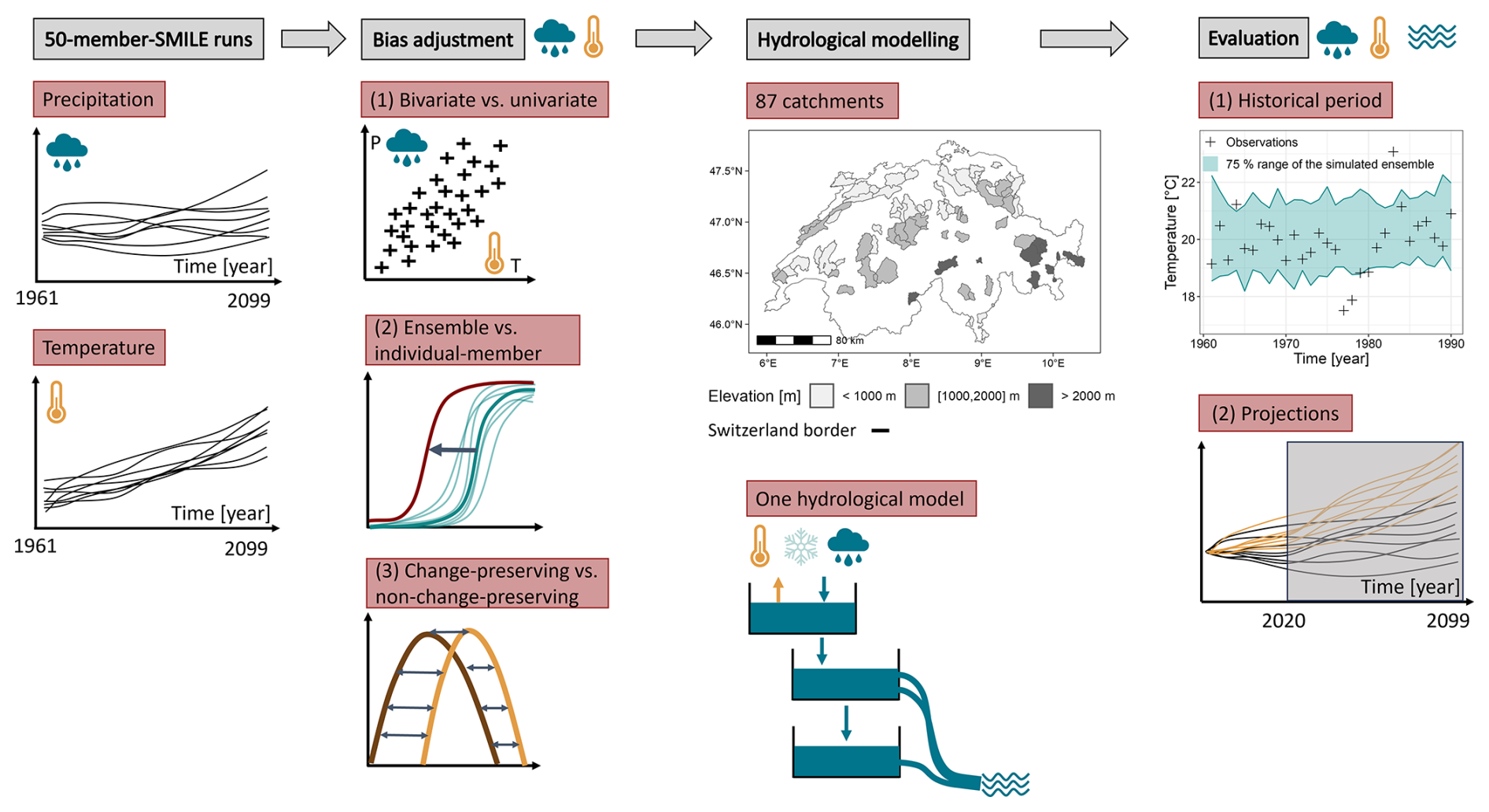
Figure 1 Flowchart describing the modelling and evaluation steps. See text for details.

2.1 Datasets

We perform analyses at the catchment scale, using 87 catchments in Switzerland (Fig. 1, Table S1 in the Supplement) that we classify into three elevation groups (Fig. 1). The catchment selection originates from the 98 “near-natural” catchments (i.e. no reservoirs are located upstream from the gauging stations) that Kraft et al. (2025) selected from the CAMELS-CH dataset (Höge et al., 2023). We do not include catchments with a predominant influence of glaciers on streamflow (11 catchments), which we do not take into account in the hydrological modelling process. This catchment selection covers a wide range of hydrological regimes over Switzerland.

We use two datasets for our experiments: (1) climate simulations from a SMILE and (2) observations, which we use to calibrate the hydrological model and to adjust the biases of the climate simulations. As observations, we use gridded daily 2 km data for precipitation and temperature between 1961 and 2020 that originate from a spatial analysis of data measured at rain gauges and temperature stations (RhiresD and TabsD; Frei and Schär, 1998; Frei, 2013; MeteoSwiss, 2019a, b). As climate simulations, we use precipitation and temperature data from the 50-member CRCM5-LE from the ClimEx experiment (Canadian Regional Climate Model version 5 (CRCM5) large ensemble; Leduc et al., 2019). This large ensemble was generated by dynamically downscaling the 50-member CanESM2-LE (Canadian Earth System Model version 2 large ensemble; Fyfe et al., 2017; Kirchmeier-Young et al., 2017) with the regional climate model CRCM5 (v.3.3.1; Martynov et al., 2013; Šeparović et al., 2013) to the EURO-CORDEX 0.11° grid (≈ 12 km). The simulations were driven with observed anthropogenic (greenhouse gas emissions, aerosols and land cover) and natural (solar and volcanic influences) forcings over the historical period (1950–2005) and with the RCP8.5 scenario (Meinshausen et al., 2011) from 2006 to 2099. We aggregate the original 1-hourly simulations to the daily time step (24 h sum for precipitation and 24 h average for temperature) for each grid cell and extract 389 grid cells over Switzerland.

2.2 Bias adjustment

We adjust the systematic biases of the RCM-SMILE using a selection of three bias adjustment methods with different types of properties, covering univariate and bivariate as well as change-preserving and non-change-preserving methods (see Table 1):

• A univariate quantile mapping (QM) method developed by Rajczak et al. (2015) and Feigenwinter et al. (2018), which is non-change-preserving. We use the version of this method implemented in the qmCH2018 R package (Kotlarski and Rajczak, 2019), which was used to develop the Swiss climate projections for the CH2018 project (Sørland et al., 2020).

• The “Cumulative Distribution Function – Transform” (CDF-t) method developed by Michelangeli et al. (2009) and Vrac et al. (2012). CDF-t is a univariate quantile mapping method that takes into account potential changes in the distribution of the adjusted variable (i.e. precipitation or temperature) between the historical and the projected period (change-preserving). We use the version implemented in the SBCK R package (Robin, 2023).

• The “Rank Resampling for Distributions and Dependences” (R2D2) method developed by Vrac (2018). R2D2 is a multivariate bias adjustment method that preserves the simulated change in the univariate distribution but not the dependence. In our study, we use the term “bivariate” to refer to the grid-cell-by-grid-cell adjustment of the dependence between precipitation and temperature. R2D2 first adjusts the marginal values of each variable's distribution using the CDF-t method and then performs a reordering of the rank structure to adjust the dependence between precipitation and temperature based on the observed dependence. We use the version implemented in the SBCK R package (Robin, 2023). Both precipitation and temperature are used as “multidimensional conditioning dimensions” to maintain some rank chronology (see Sect. 3.2 of Vrac and Thao, 2020).

Table 1 List of the three bias adjustment methods tested: QM, CDF-t and R2D2. The last two columns encompass five bias adjustment strategies.

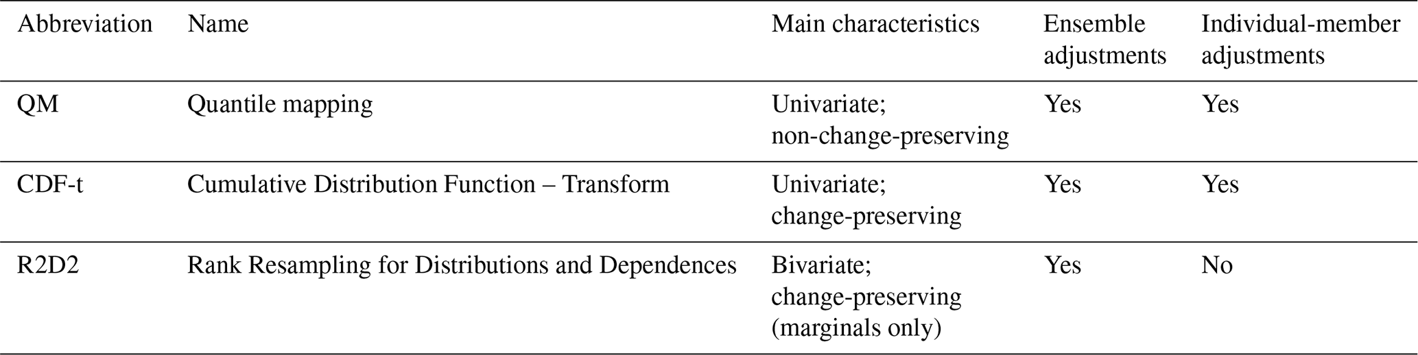
A comparison between CDF-t and QM will allow us to quantify the difference between change- vs. non-change-preserving methods, and a comparison between R2D2 and CDF-t will allow us to quantify the difference between univariate and bivariate bias adjustments.

We adjust the precipitation and temperature biases of the RCM-SMILE at its native resolution (12 km) to avoid introducing artefacts resulting from additional downscaling (e.g. overestimation of extremes and overcorrection of the drizzle effect for area means; Maraun, 2013). Applying the bias adjustment at the catchment scale would result in mixing the bias adjustment with upscaling for large catchments and downscaling for small catchments. To do so, we first upscale the precipitation and temperature observations to the RCM-SMILE resolution using conservative remapping with the Climate Data Operators (CDO) software (Schulzweida, 2023). We then run the adjustments grid cell by grid cell. Last, we calculate catchment averages of precipitation and temperature to generate inputs for the lumped hydrological model (see Sect. 2.3). However, we perform all analyses at the catchment scale (except for the correlation analysis; see Sect. 3.1) in order to look at the impact of the choice of bias adjustment strategies on hydrologically meaningful variables.

We first apply all of the above-mentioned methods by adjusting the entire ensemble together (“ensemble adjustment”). To perform the ensemble adjustment, we use the “Bias Correction ensemble” method (BCens) described in Vaittinada Ayar et al. (2021), which adjusts each member based on adjustment factors derived from the difference between the ensemble distribution (all members pooled together) and the observations. Then, we test a second method to adjust the ensemble that consists of adjusting each member individually (“individual-member adjustment”). Here, we adjust each member based on adjustment factors derived from the difference between the respective individual-member distribution and the observations. To reduce the complexity of the analyses, we apply individual-member adjustment only to QM and CDF-t (see Table 1).

To assess the advantages and disadvantages of each adjustment strategy, we conduct two experiments. First, we perform a calibration/evaluation test over the historical period to assess the performance of the bias adjustment strategies. For this, we calibrate the bias adjustment strategies for two sub-periods: 1961–1990 (P1) and 1991–2020 (P2). We use the adjustment factors derived from P1 to adjust the climate simulations of P2 and the adjustment factors derived from P2 to adjust the climate simulations of P1 (cross-evaluation test). Note that P2 includes both historical and scenario data, but this should not affect the results of our study. Second, we calibrate the bias adjustment strategies for 1991–2020 and apply them to future projections of precipitation and temperature between 2021 and 2099 to evaluate change preservation.

To account for the seasonal cycle, we perform bias adjustment for each month individually, based on a 3-month distribution centred on the month of interest (Cannon et al., 2015). To correct for dry days in the precipitation time series, we apply a threshold of 0.05 mm d⁻¹ for the QM method (reference setup for quantile mapping) and the “Singularity Stochastic Removal” method of Vrac et al. (2016) for CDF-t and R2D2 (reference setup for these methods), which corrects precipitation occurrences by replacing precipitation values below a specific threshold with randomly selected and extremely small values.

Then, for the second experiment focusing on future projections, we adjust the biases over a 30-year sliding window, moving forward every 10 years, as done in Hempel et al. (2013), Vrac et al. (2016), Cannon (2017) and Meyer et al. (2019). For each time window, the central 10 years of adjusted data are saved. For example, this method adjusts the biases for 2040–2049 based on the adjustment factors calculated for 2030–2059.

2.3 Hydrological modelling

We run the TUW model (Parajka et al., 2007) to simulate and project streamflow at the outlet of 87 catchments with the precipitation and temperature time series from the different bias adjustment strategies. The TUW model is a lumped rainfall–runoff model based on the HBV model structure (Bergström and Forsman, 1973) and takes time series of precipitation, temperature and potential evapotranspiration as inputs. We use the model version implemented in the TUWmodel R package (Viglione and Parajka, 2020) and estimate potential evapotranspiration using the air-temperature-based formula provided by Oudin et al. (2005). The TUW model has 15 free parameters, which we calibrate for each catchment using time series of meteorological and streamflow observations (Federal office for the Environment, 2024). We calibrate the parameters over the period 1993–2011 using the Kling–Gupta efficiency (KGE) index (Gupta et al., 2009) as the objective function, and we apply a warm-up period of 2 years before the calibration period. The model shows reasonable performance for high flows in extrapolation between 2011 and 2019 over the catchment set, with a median KGE value of 0.81 (0.75 for the lower quartile and 0.84 for the upper quartile; Fig. S10). The model shows lower performance for low than for median and high flows (Fig. S10), which is a common limitation of hydrological models (Bruno et al., 2024). For this reason, we check the robustness of our results with respect to the choice of the hydrological model by using a second model with a different structure (Cemaneige-GR5J; Fig. S3; Le Moine, 2008; Valéry et al., 2014; Coron et al., 2020).

2.4 Evaluation

We evaluate the hydrological simulations driven by the SMILE both for the historical period based on the calibration/evaluation sub-periods (1961–1990 and 1991–2020) and for three future periods (2021–2050, 2051–2080, 2081–2099) compared to the reference period (1991–2020) using different percentiles representing low-flow (1st), high-flow (99th) and normal flow (median) conditions. We use the same percentiles to evaluate temperature but the 90th (moderate precipitation) and the 99th (extremes) percentiles for precipitation, as it follows a right-skewed distribution.

We first evaluate the performance of the different bias adjustment strategies (QM, CDF-t and R2D2; ensemble vs. individual adjustments) over the historical period (calibration/evaluation experiment). When adjusting a SMILE, we do not want the adjusted statistical properties of each member to be close to those of the observations, as this would imply a reduced ensemble spread (i.e. internal variability). Instead, we want to remove systematic biases so that the statistical properties for the different members of the ensemble contain those of the observations over the climatic sub-periods (i.e. P1 and P2). In other words, we want to obtain an unbiased ensemble (systematic biases) instead of unbiased members, which would imply removing the fluctuations due to internal climate variability. To test this, we use the ensemble evaluation framework developed in Suarez-Gutierrez et al. (2021) and Wood et al. (2021). The aim of this framework is to evaluate the biases and the variability of ensemble climate simulations by comparing statistical features of observations to those of the ensemble runs. To apply this framework, we first calculate a yearly percentile for a given variable (e.g. 99th temperature percentile) for each sub-period, catchment, bias adjustment strategy and member. We calculate the same statistic for the observations, shown as black markers in the top-right panel of Fig. 1. Then, we calculate the central 75 % confidence interval of the yearly percentile across the members for each year (blue interval in the top-right panel of Fig. 1). The 75 % criterion calculates the proportion of observed statistics that fall within the 75 % confidence interval. The ideal value for this criterion is 0.75, as we expect 75 % of the observed statistics to fall within the simulated 75 % confidence interval. For the example shown in the top-right panel of Fig. 1, the value of this criterion is 0.83, as 5 out of 30 years of observations fall outside the 75 % range of the ensemble. This criterion evaluates both the bias and the variability of the ensemble (for more details, see Suarez-Gutierrez et al., 2021; Wood et al., 2021). To evaluate the inter-member variability of the ensemble, we calculate the spread between members for a given percentile and a given variable (standard deviation for temperature and coefficient of variation for precipitation). To evaluate the performance of bias adjustment for streamflow simulations, we use the streamflow time series simulated by the hydrological model with observed precipitation and temperature inputs as our control run to calculate the 75 % range criterion. We use simulated instead of observed streamflow to reduce the dependence of our results on uncertainties in hydrological modelling. This means that the performance of the hydrological model in simulating streamflows should not significantly impact the results. To assess whether the performance distributions are significantly different across bias adjustment strategies, we perform the Wilcoxon rank test (Wilcoxon, 1945) at a significance level of 0.05 (non-paired; two-sided). Finally, for conciseness purposes, we combine both climate sub-periods (P1 and P2) in the presentation of the results, which means that “calibration” and “evaluation” include both P1 and P2.

In order to assess the impact of change-preserving and ensemble adjustments on future climate and streamflow projections, we calculate several indicators. First, we calculate the discrepancy between the signal projected by the unadjusted ensemble and the signal projected by the ensemble adjusted by the non-change-preserving bias adjustment method (QM) or the change-preserving bias adjustment method (CDF-t) for precipitation and temperature (ensemble adjustment method only). To do this, we calculate the signal (difference) between the future period (e.g. 2081–2099) and the reference period (1991–2020) for a given percentile (e.g. 1st percentile of temperature) and a given member. We then calculate the average signal across members. To ensure consistency with the analyses performed on the historical period, we calculate annual percentiles averaged over the climate period of interest. We calculate an absolute signal for temperature and a relative signal for precipitation. Second, we calculate the difference between the signal from the adjusted ensemble and the signal from the raw (i.e. unadjusted) ensemble. This allows us to assess whether the two adjustment methods preserve the signal of the climate model.

Second, to further assess the impacts of change-preserving vs. non-change-preserving and individual-member vs. ensemble adjustments on climate and streamflow projections, we calculate indicators that are often used in studies on climate change impacts on extremes, namely the signal-to-noise ratio and the time-of-emergence (e.g. Muelchi et al., 2021a, b). The signal-to-noise ratio indicates how the changes (signal) compare to the noise of the ensemble (standard deviation of the signal projected by the different members). We calculate the signal-to-noise ratio for precipitation, temperature and streamflow percentiles and compare the results between bias adjustment strategies and between catchments. The time-of-emergence is defined as the year when the signal-to-noise ratio exceeds 1 or falls below −1 (and remains so) and indicates when changes emerge from the noise. To calculate the signal-to-noise ratio values used to estimate the time-of-emergence, we apply a centred 20-year moving window (moving every year from the historical period to the end of the century). We analyse only the results for the precipitation and streamflow time-of-emergence, as the time-of-emergence for temperature is reached very early for most catchments in our dataset. In order to compare the time-of-emergence values between the bias adjustment strategies, we classify the catchments into three elevation groups (<1000 m, [1000,2000] m and >2000 m; Fig. 1).

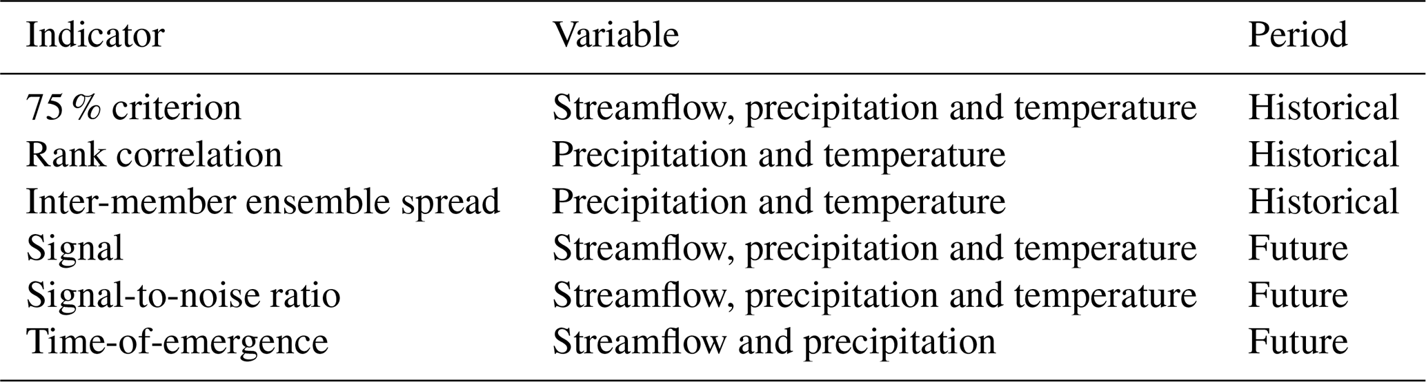
We summarize all the indicators used for the evaluation in Table 2.

Table 2 List of the indicators used to evaluate the bias adjustment strategies.

3 Results

3.1 Performance of the bias adjustment methods in the historical period

3.1.1 Streamflow

We first examine the performance of the three bias adjustment methods (QM, CDF-t and R2D2), using the ensemble adjustment method, for streamflow simulations in the historical period (Fig. 2).

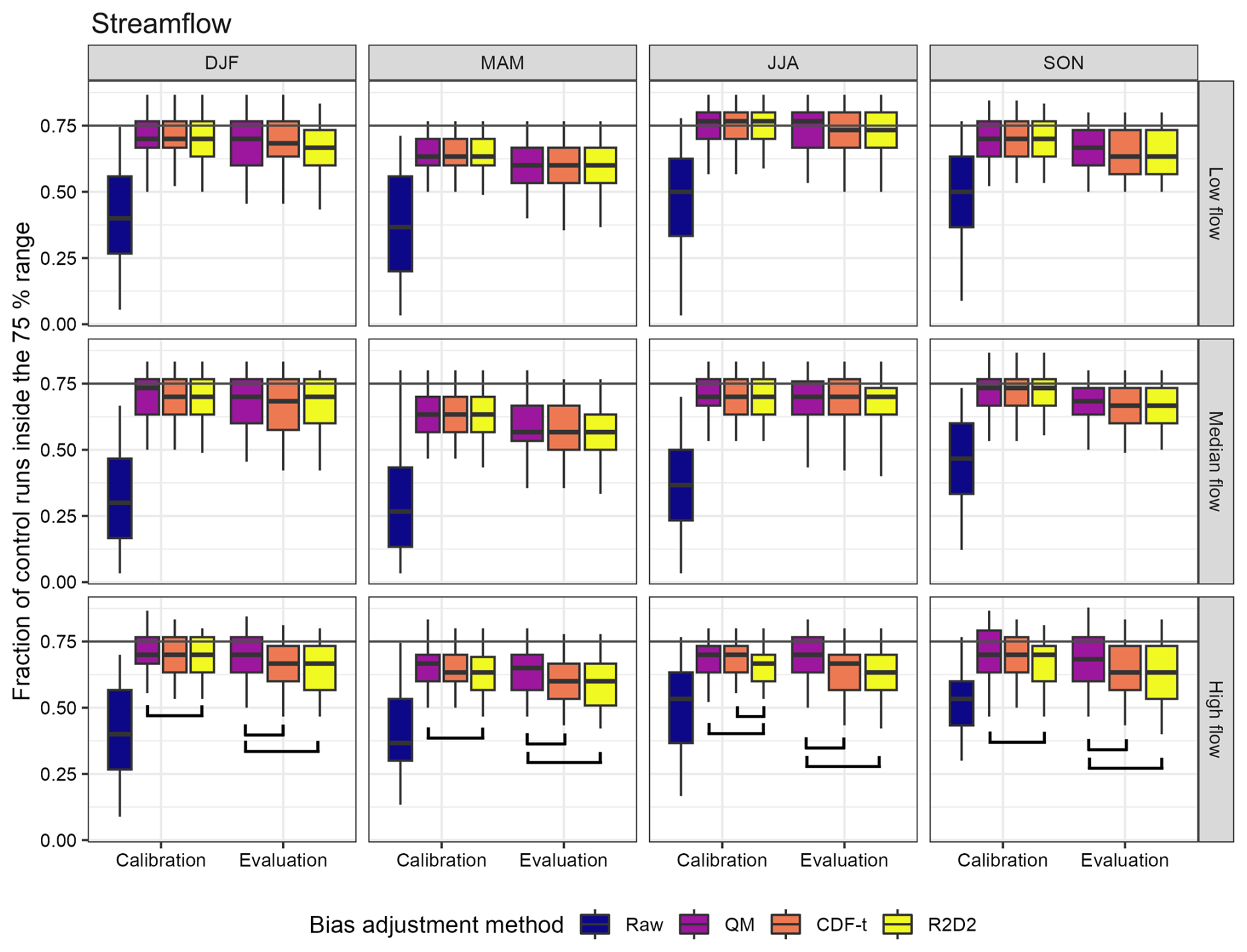
Figure 2 Ability of the three bias adjustment methods and the unadjusted ensemble (raw) to reproduce streamflow statistics of the control runs (streamflow time series simulated by the hydrological model with observed precipitation and temperature inputs) for the 87 catchments. The fraction of control runs within the simulated 75 % confidence interval was calculated for four seasons (December/January/February, March/April/May, June/July/August, September/October/November) and three streamflow percentiles (1st, 50th and 99th). The optimum value of the performance criterion is 0.75. QM is the univariate non-change-preserving method, CDF-t is the univariate change-preserving method and R2D2 is the bivariate change-preserving method. All methods were run using the ensemble adjustment method. Calibration and evaluation combine both climatic sub-periods. Statistically different distributions are connected by black lines. These black lines are not plotted for the raw ensemble because its distribution significantly differs from all bias-adjusted distributions.

As expected, the streamflow simulations driven by the unadjusted (raw) ensemble have large biases in the historical period (cf. position of the dark blue boxplots compared to the optimum value of the performance criterion, i.e. 0.75). All bias adjustment methods significantly reduce the streamflow biases compared to the raw ensemble across catchments, seasons and streamflow percentiles, although we find a drop in performance when moving from the calibration to the evaluation periods. The performance of all bias adjustment methods varies by season, with higher performance in winter (DJF) and summer (JJA) and lower performance in spring (MAM) and autumn (SON). There are no significant differences between the performance distributions of univariate (CDF-t) and bivariate (R2D2) adjustments for all seasons and streamflow percentiles (except for high flow in summer for the calibration periods, where univariate adjustments lead to higher performance). Additionally, we find similar results for snow water equivalent simulations (see Fig. S1 in the Supplement). In contrast, the univariate non-change-preserving method (QM) has higher performance for high flow than the univariate change-preserving method (CDF-t) for both evaluation periods and all seasons. The same differences are found between bivariate change-preserving (R2D2) and univariate non-change-preserving (QM) adjustments. Additionally, we find no obvious spatial patterns between the bias adjustment methods (Fig. S2). These findings are independent of the choice of the hydrological model (see Fig. S3 in the Supplement) and of the confidence interval chosen (Fig. S11).

3.1.2 Dependence between precipitation and temperature

These results highlight that there are no significant improvements in streamflow simulations from applying bivariate over univariate adjustments (i.e. between R2D2 and CDF-t). We now investigate possible reasons for this finding, which are (1) the ability of the unadjusted ensemble to reproduce the observed dependence between precipitation and temperature and (2) the ability of the bias adjustment methods to adjust this dependence. By construction, unlike the univariate method (CDF-t), the bivariate method (R2D2) is explicitly designed to adjust this dependence. To check how well the bivariate method captures the observed precipitation–temperature dependence compared to the univariate method and the raw ensemble, we look at the Spearman rank correlation between precipitation and temperature for the 389 adjusted cells (Fig. 3; here, the results of QM are not presented, as they follow those of CDF-t). The correlations between precipitation and temperature simulated by the raw ensemble are already close to the observed correlations for a large number of cells (Fig. 3A and B). However, the spatial variability of the correlation values is smoother than the one of the observations, and negative correlations are more pronounced over high elevations, about 0.1 larger in absolute terms. The univariate method (CDF-t) removes the spatial smoothing of the raw ensemble and already brings the values closer to the observations (Fig. 3C). The bivariate adjustment (R2D2) further improves these correlations (Fig. 3D) but does not lead to any substantial improvements compared to CDF-t.

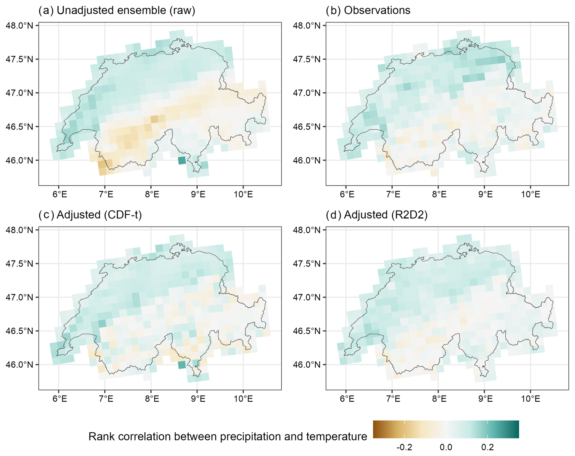
Figure 3 Spearman rank correlation between precipitation (pr) and temperature (tas) on wet days (pr > 1 mm d⁻¹) and for days with transition temperatures between −2 and 2 °C. CDF-t is the univariate change-preserving method, and R2D2 is the bivariate change-preserving method. The raw ensemble is the unadjusted ensemble. All methods were run using the ensemble adjustment method. The results are shown for both evaluation sub-periods combined (1961–2020) and without any seasonal distinction made.

3.1.3 Ensemble adjustments and interannual vs. inter-member variability

The results presented in Fig. 2 show that the univariate non-change-preserving adjustments (QM) result in higher high-flow performance than the univariate change-preserving adjustments (CDF-t). We now examine whether the choice of the ensemble adjustment method (individual-member vs. ensemble; Fig. 4A and B) is linked to this result by examining precipitation and temperature performance. We find no difference in precipitation and temperature performance between non-change-preserving bias adjustment (QM) and change-preserving bias adjustment (CDF-t) and between individual-member and ensemble adjustments for the 90th precipitation percentile, and for the 50th and 99th temperature percentiles, for both the calibration and evaluation periods. We obtain a different pattern for the 99th precipitation percentile and for the 1st temperature percentile. While there are no significant differences between individual and ensemble adjustments for the QM method for neither calibration nor evaluation, the performance distributions of CDF-t are significantly different in evaluation for both ensemble adjustment methods compared. CDF-t in ensemble mode leads to a degraded performance in the simulation of the tail of the precipitation distribution and in the simulation of the left tail of the temperature distribution. In fact, there is a reduction in performance by 6 % for precipitation and by 10 % for temperature compared to individual-member adjustments (Fig. 4), i.e. fewer observations fall within the simulated 75 % confidence interval (cf. top-right panel of Fig. 1).

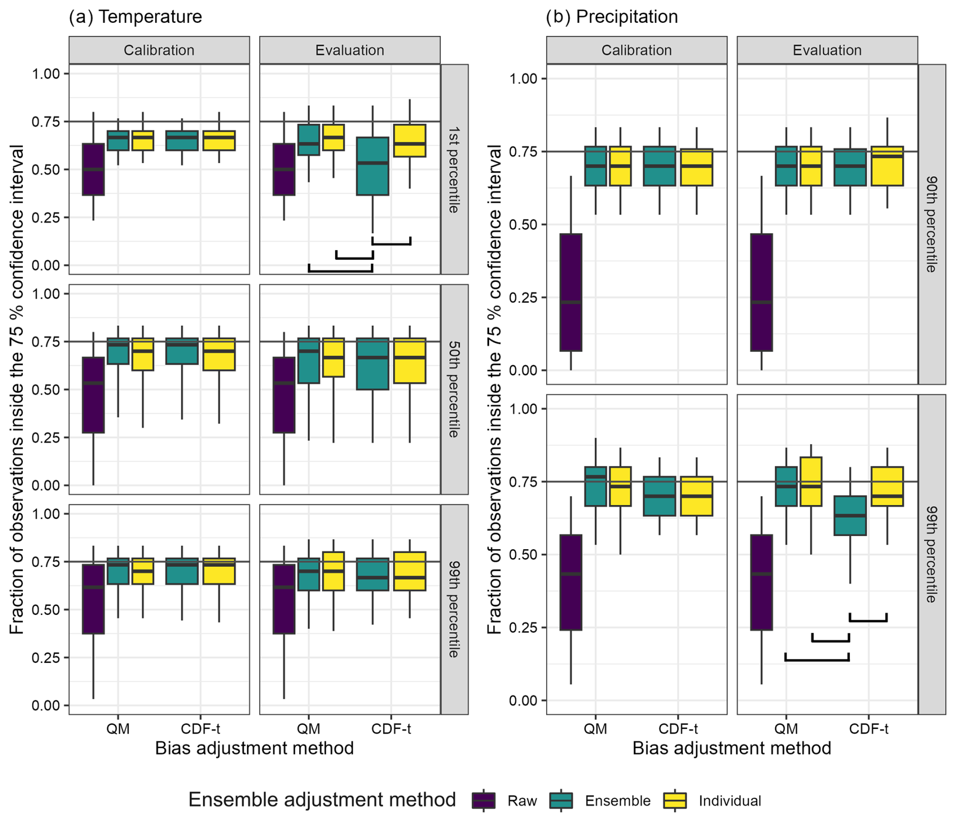
Figure 4 Distribution of temperature (a) and precipitation (b) performance for the 87 catchments, different bias adjustment strategies, three temperature percentiles (i.e. the 1st, 50th and 99th percentiles), and two precipitation percentiles (i.e. the 90th and 99th percentiles). Performance is assessed with the fraction of observations falling inside the simulated 75 % confidence interval. The optimum value of the performance criterion is 0.75. QM is the univariate non-change-preserving method, and CDF-t is the univariate change-preserving method. Raw is the unadjusted ensemble. Calibration and evaluation combine both climatic sub-periods. Statistically different distributions are connected by black lines. These black lines are not plotted for the raw ensemble because its distribution significantly differs from all bias-adjusted distributions.

While individual-member bias adjustments lead to unbiased simulations when looking at interannual extremes (Fig. 4), they could reduce the variability of the ensemble. We investigate this aspect by calculating the inter-member variability of the ensemble (the standard deviation for temperature and the coefficient of variation for precipitation) for the temperature and precipitation percentiles used in Fig. 4 (Fig. 5).

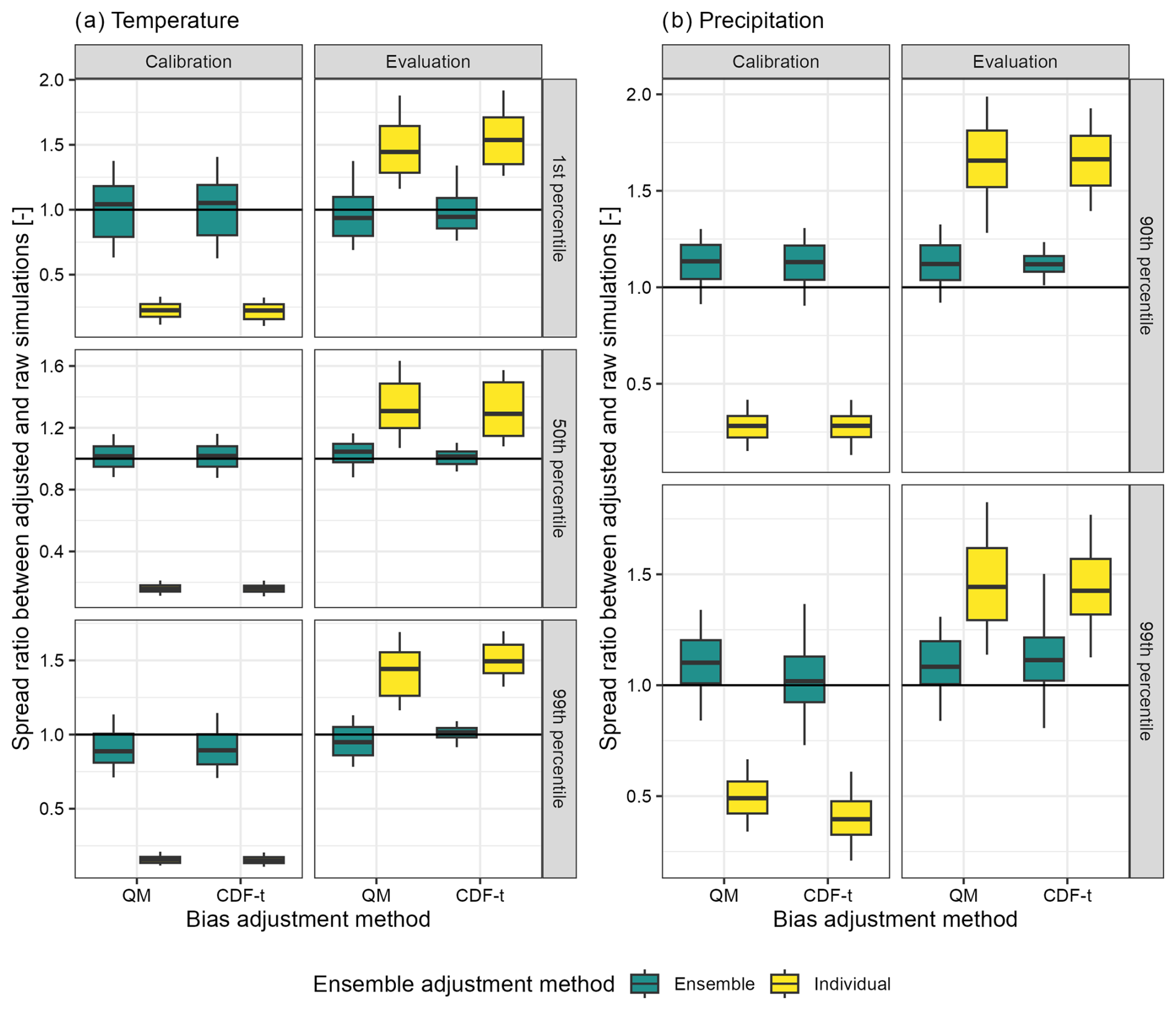
Figure 5 Ratio between the variability of the ensemble after adjustments and the variability of the raw (unadjusted) ensemble per catchment for (a) three annual temperature percentiles (i.e. the 1st, 50th and 99th percentiles) and (b) two annual precipitation percentiles (i.e. the 90th and 99th percentiles) for the 87 catchments. The optimum value of this ratio is 1. A value above 1 indicates an overestimation of the variability, and a value below 1 indicates an underestimation of the variability. The temperature variability is calculated as the standard deviation between members for a given percentile and the precipitation variability as the coefficient of variation between members for a given percentile.

Individual-member adjustments clearly reduce the variability of the ensemble for the calibration periods (median values of the spread ratio are always lower than 0.25 for temperature and 0.5 for precipitation) but increase the variability of the ensemble for the evaluation periods (median values of the spread ratio are always higher than 1.3 for temperature and 1.4 for precipitation) for both temperature and precipitation percentiles and for both change-preserving and non-change-preserving methods. In contrast to individual-member adjustments, ensemble adjustments preserve the variability of the ensemble during both calibration and evaluation for most catchments and for both temperature and precipitation (median spread ratio is close to 1 in most cases). Note that for ensemble adjustments, the variability of the precipitation ensemble is, in most cases, larger than the raw variability, but to a much smaller extent than for individual-member adjustments.

3.2 Future climate and hydrological extremes

The analysis for the historical period shows that the choice of individual-member vs. ensemble bias adjustment and change-preserving vs. non-change-preserving bias adjustment impacts streamflow, temperature and precipitation performance, as well as precipitation and temperature variability. These differences may lead to discrepancies in the projection of future climate and hydrological extremes. Therefore, we investigate the differences in the projected climate signal and the signal-to-noise ratio due to the choice of the bias adjustment strategy compared to the signal projected by the raw (unadjusted) ensemble that we want to preserve. Further, we assess the impact of this choice on the time-of-emergence of both precipitation and streamflow.

3.2.1 Preservation of changes in temperature and precipitation

Figure 6 illustrates the differences in the projected temperature (A) and precipitation (B) signals for the change-preserving and non-change-preserving bias adjustments compared to the unadjusted projections (i.e. the raw ensemble). We obtain up to 2.5 °C differences in projected low temperature changes (1st percentile) for the non-change-preserving bias adjustment (QM), with an underestimation of the raw warming at low elevations and an overestimation at high elevations. In contrast, the change-preserving adjustments (CDF-t) do not induce such differences in low temperature changes, with only up to a 1 °C difference for some catchments but no apparent elevation dependence. For median and high temperatures (99th percentile), we find smaller differences for both bias adjustment methods, except for a few high-elevation catchments where the non-change-preserving adjustments overestimate temperature changes by up to 1 °C. While the non-change-preserving adjustments clearly lead to temperature change discrepancies (1st percentile) compared to the change-preserving method, the results are less clear for precipitation changes. Indeed, we find differences in precipitation changes of up to 12 percentage points (absolute delta signal values) for both change-preserving and non-change-preserving adjustments and for both the 90th and 99th precipitation percentiles. Specifically, moderate precipitation (90th percentile) is mostly underestimated (delta signal values ranging from −3 %pt to −12 %pt), and extreme precipitation is overestimated in low-elevation catchments (up to 6 %pt) and both overestimated (up to 6 %pt) and underestimated (up to −12 %pt) in high-elevation catchments.

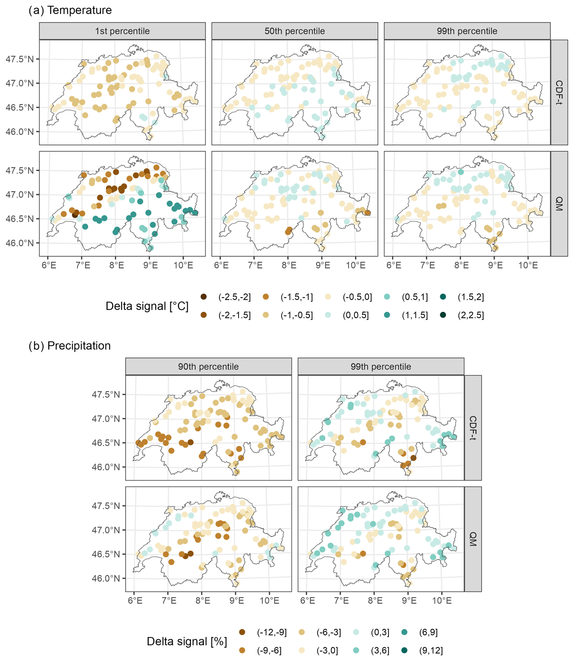
Figure 6 Climate signal differences between bias-adjusted projections and raw projections at the end of the century (2081–2099 vs. 1991–2020) for (a) the temperature signal for three percentiles and (b) the precipitation signal for two percentiles. Results are shown for 87 catchments and the ensemble adjustment method. QM is the univariate non-change-preserving method, and CDF-t is the univariate change-preserving method.

We now investigate whether these differences in the change signals together with the choice of individual-member vs. ensemble bias adjustment lead to differences in signal-to-noise ratio values (cf. differences in the signal-to-noise ratio between adjusted and unadjusted projections; Fig. 7).

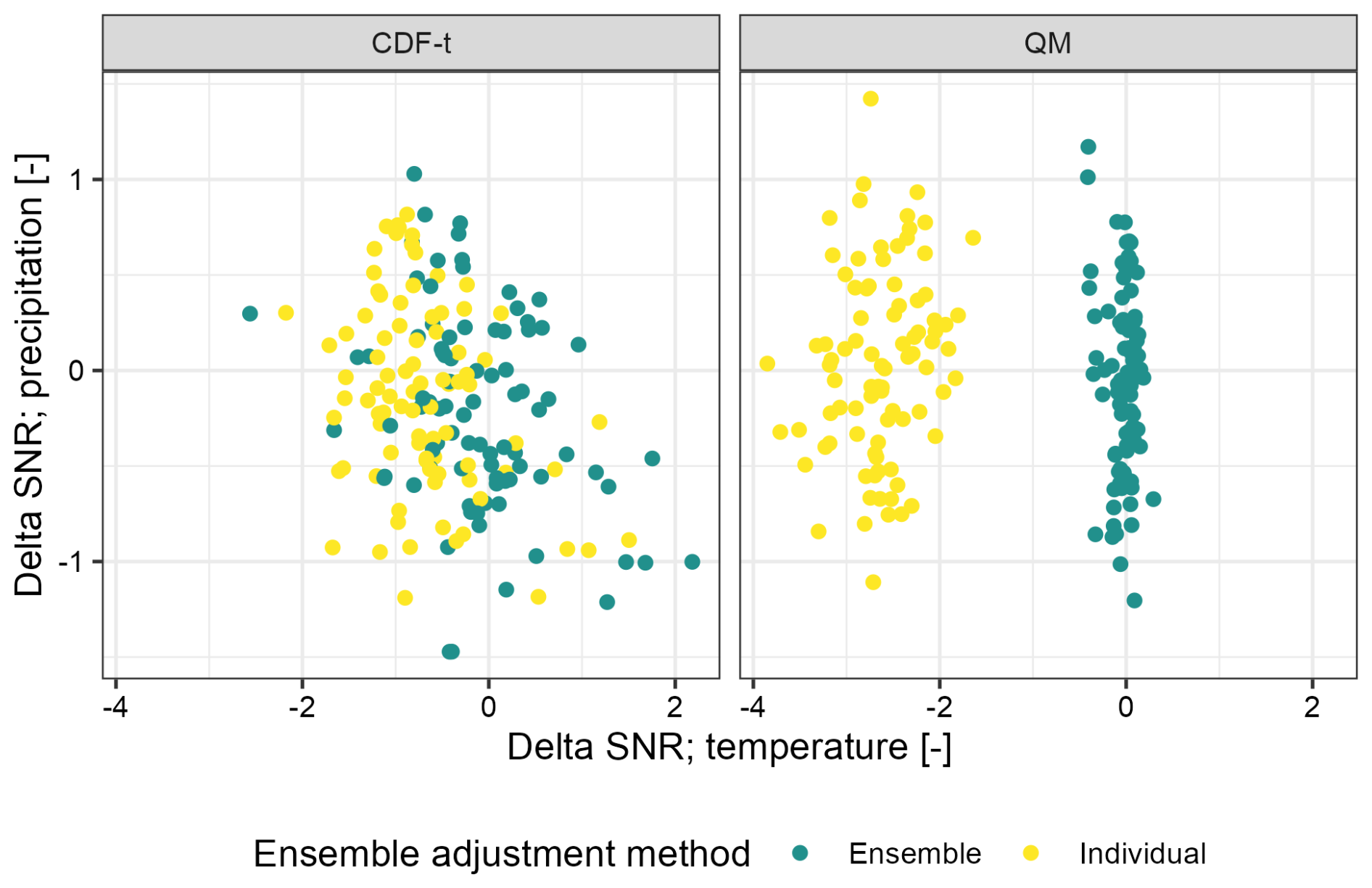
Figure 7 Catchment differences in temperature and precipitation signal-to-noise ratio (SNR) between bias-adjusted projections and raw projections for four adjustment strategies. Results are shown for 87 catchments and the period (2081–2099) compared to (1991–2020) and the 99th percentile. QM is the univariate non-change-preserving method, and CDF-t is the univariate change-preserving method.

We obtain large catchment differences in signal-to-noise ratio values (delta values up to 4 units) for high temperatures (99th percentile) between the non-change-preserving bias adjustment (QM) in individual-member mode and the unadjusted ensemble (raw projections). These differences in the signal-to-noise ratio range from 1.5 to 4 units in 2081–2099. In contrast, when the ensemble bias adjustment is combined with the non-change-preserving bias adjustment, the differences in the temperature signal-to-noise ratio are smaller (delta values up to 0.5 unit). This indicates that the individual-member adjustment significantly changes the temperature signal-to-noise ratio compared to the ensemble adjustments, when combined with non-change-preserving bias adjustments. In contrast, the change-preserving method (CDF-t) shows the same order of magnitude of temperature signal-to-noise ratio differences between individual-member and ensemble bias adjustments. For precipitation, we obtain large delta values of precipitation signal-to-noise ratios for some catchments (delta values up to 1.5 units), regardless of the strategy chosen (change-preserving, non-change-preserving, individual-member and ensemble). Overall, these results clearly show that there are interactions between the choice of change-preserving vs. non-change-preserving bias adjustment and individual-member vs. ensemble bias adjustment in projecting future climate extremes.

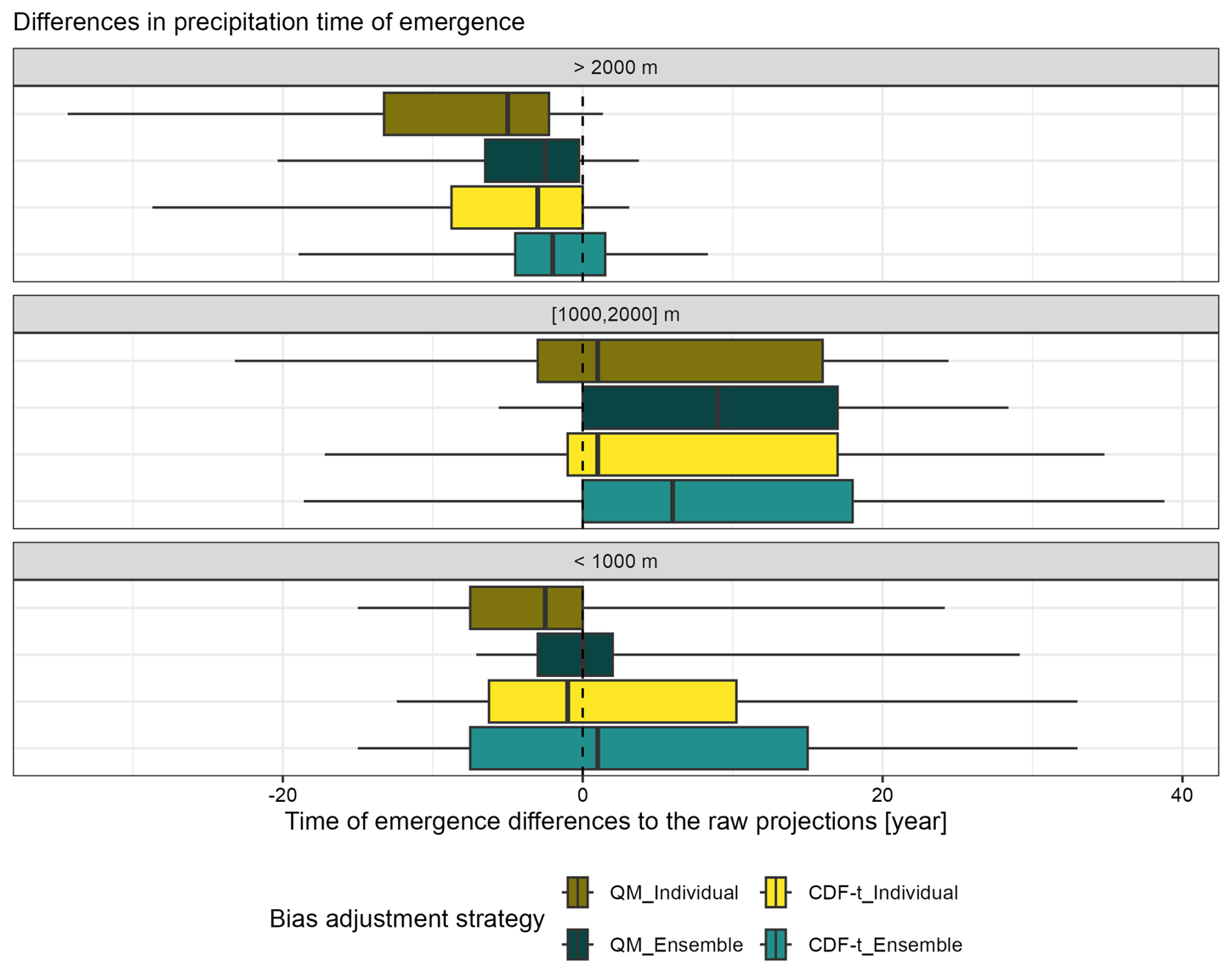
Figure 8 Distribution of catchment differences in precipitation time-of-emergence between bias-adjusted projections and raw projections for four bias adjustment strategies. The distributions are shown for 87 catchments classified into three elevation bands (< 1000, 1000–2000 and >2000 m) and the 99th precipitation percentile. QM is the univariate non-change-preserving method. CDF-t is the univariate change-preserving method.

These differences in climate signals and the signal-to-noise ratio lead to differences in the time-of-emergence compared to the unadjusted ensemble (raw projections). In Fig. 8, we investigate whether these differences in time-of-emergence in extreme precipitation (99th percentile) vary with the choice of bias adjustment (change-preserving, non-change-preserving, individual-member and ensemble) and with catchment elevation. At high elevations (>2000 m), we find larger differences in the time-of-emergence (relative to the unadjusted ensemble) for individual-member than for ensemble bias adjustment. This is the case for both change-preserving and non-change-preserving bias adjustments (brown vs. dark-green and yellow vs. light-green boxplots), with larger differences for non-change-preserving bias adjustment. In addition, individual-member bias adjustment leads to earlier precipitation time-of-emergence than ensemble bias adjustment (median difference of −2 years for non-change-preserving adjustments and −1 year for change-preserving adjustments). At intermediate elevations (between 1000 and 2000 m), the differences in the time-of-emergence are large for all bias adjustment strategies, but individual-member bias adjustment leads to earlier time-of-emergence than ensemble bias adjustment (median difference of +8 years for non-change-preserving adjustments and +4 years for change-preserving adjustments). At low elevations (<1000 m), the differences in the time-of-emergence are larger for the change-preserving adjustments than for the non-change-preserving adjustments. Again, individual-member bias adjustment leads to earlier time-of-emergence than ensemble bias adjustment (median difference of −3 years for non-change-preserving adjustments and −2 years for change-preserving adjustments). However, the differences between the time-of-emergence distributions are not statistically different (as assessed by a Wilcoxon rank test (Wilcoxon, 1945) at a significance level of 0.05; non-paired; two-sided), except between individual non-change-preserving adjustments (QM_Individual) and ensemble non-change-preserving adjustments (QM_Ensemble) at low elevation. Nevertheless, the results clearly show that bias adjustment generally leads to changes in the time-of-emergence compared to the unadjusted ensemble and that individual-member bias adjustment leads to earlier precipitation time-of-emergence than ensemble bias adjustment.

3.2.2 Impact on streamflow changes

The differences in future precipitation and temperature extremes between bias adjustment strategies may affect future streamflow extremes. To assess to which degree this is the case, we analyse the differences in streamflow time-of-emergence projected by the hydrological model driven by climate simulations adjusted by the four bias adjustment strategies (change-preserving, non-change-preserving, individual-member and ensemble; Figs. 9 and 10). We first illustrate these potential differences for high flow and three catchments in our dataset (Fig. 9). As these differences in streamflow time-of-emergence can originate from large variations in the streamflow noise and signal, we show the decomposition of the signal-to-noise ratio (Fig. 9A) into signal and noise (Fig. 9B and C). We choose these three examples because they illustrate three different cases of time-of-emergence differences originating from differences in signal and noise. For the Grosstalbach River at Isenthal, located in central Switzerland, both the choice of change-preserving (CDF-t) vs. non-change-preserving (QM) bias adjustment and individual-member vs. ensemble bias adjustment affect the high-flow signal-to-noise ratio and thus the time-of-emergence, which varies from 2050 to no time-of-emergence before 2099. This is due to a weaker signal when both change-preserving and individual-member bias adjustments are applied and more noise for change-preserving bias adjustment than for non-change-preserving bias adjustment. For the Saltina River at Brig, a tributary of the Rhône River in southern Switzerland, large differences in high-flow time-of-emergence are observed for the change-preserving bias adjustment used in combination with individual-member bias adjustment, resulting from more noise and a weaker signal. For the Seyon River at Valangin, in northwestern Switzerland, the non-change-preserving bias adjustment leads to an earlier high-flow time-of-emergence than the change-preserving bias adjustment, due to a projected high-flow signal that is stronger than for the change-preserving bias adjustment.

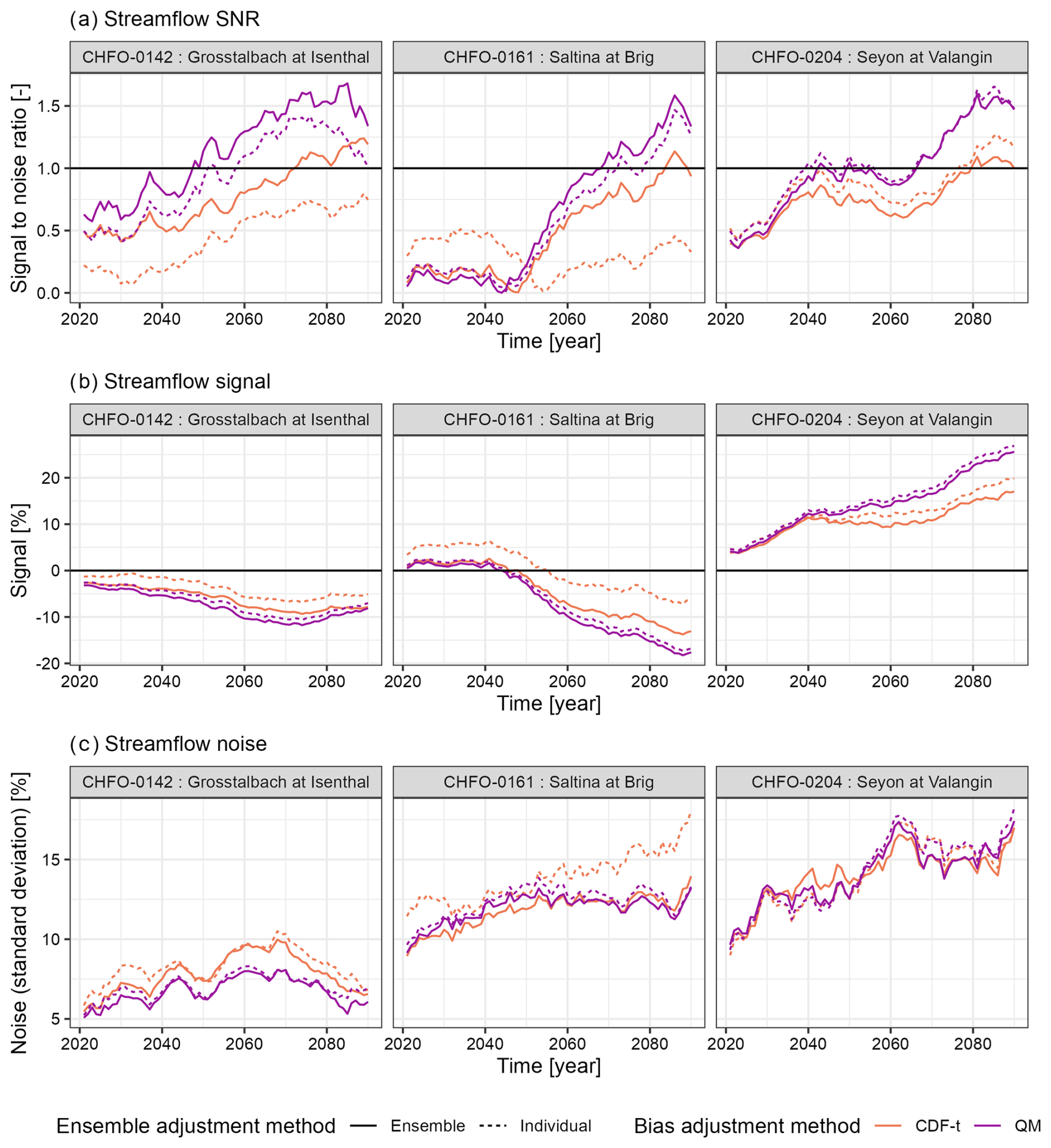
Figure 9 Impact of bias adjustment strategy on future high-flow (99th percentile) (a) signal-to-noise ratio, (b) signal and (c) noise for three catchments. The noise is expressed as a percentage because the streamflow signal is expressed in relative terms. QM is the univariate non-change-preserving method, and CDF-t is the univariate change-preserving method.

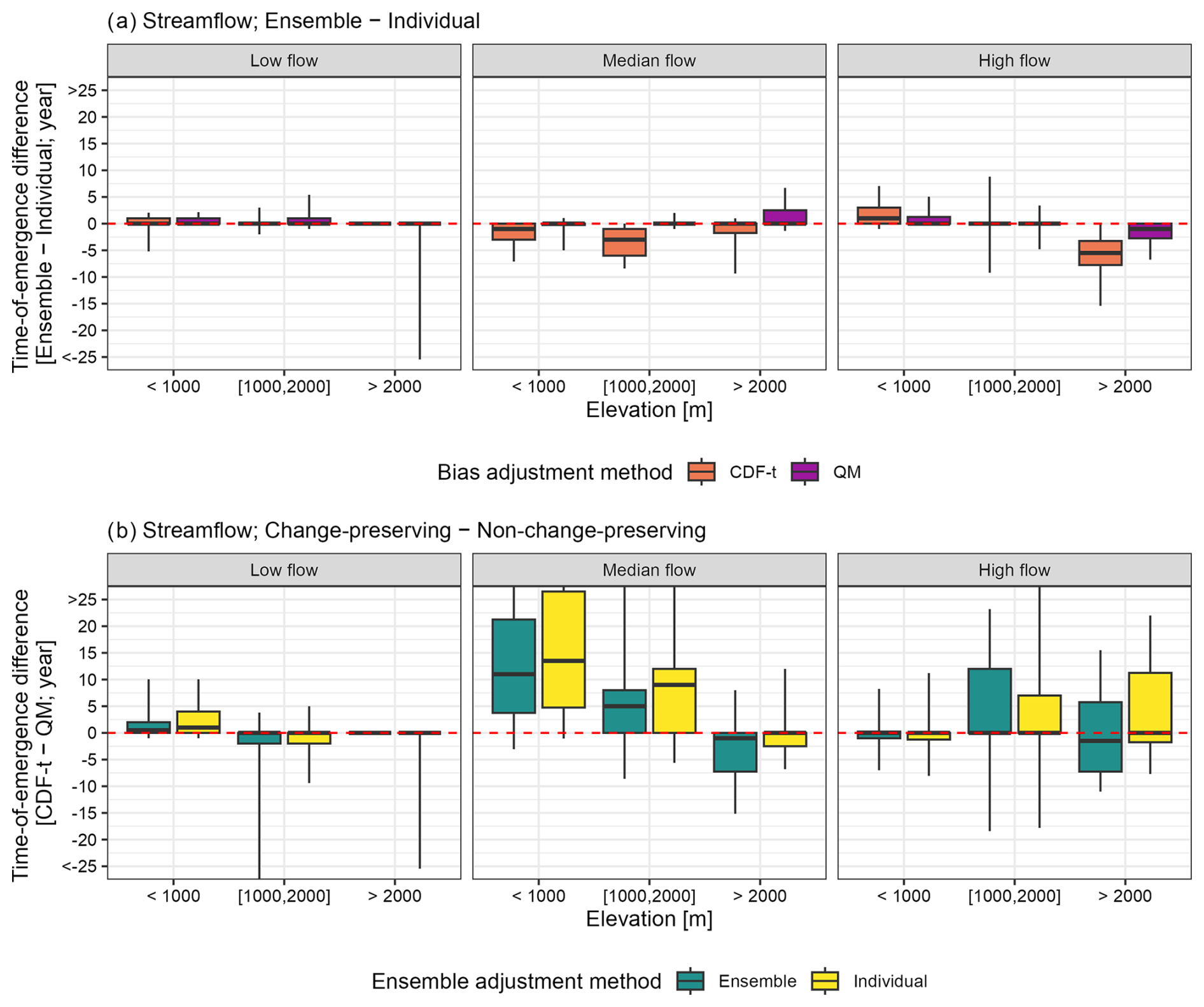
Figure 10 Streamflow time-of-emergence difference between (a) ensemble and individual-member adjustments and (b) change-preserving and non-change-preserving adjustments. The results are presented for three streamflow percentiles (1st, 50th and 99th) and 87 catchments classified into three elevation bands. QM is the univariate non-change-preserving method, and CDF-t is the univariate change-preserving method.

We now generalize these results for all catchments and low, median and high flows (10). We find no catchment differences in low-flow time-of-emergence between ensemble and individual-member adjustments (for both change-preserving (CDF-t) and non-change-preserving (QM) adjustments). However, ensemble adjustments lead to earlier time-of-emergence than individual-member adjustments for median flow at low and intermediate elevations (median differences of −1 and −3 years, respectively) and for change-preserving adjustments only (Fig. 10A). For high flows at low elevations, individual-member adjustments lead to earlier time-of-emergence than ensemble adjustments (median difference of 1 year for CDF-t) and later time-of-emergence at high elevations (median differences of 5 years for CDF-t and 1 year for QM). In that case, the differences are larger for change-preserving adjustments than for non-change-preserving adjustments. The differences in time-of-emergence between change-preserving and non-change-preserving adjustments are larger than those between individual-member and ensemble adjustments (Fig. 10B compared to A). For low flows, non-change-preserving adjustments lead to earlier time-of-emergence at low elevations (median of 1 year for ensemble adjustments and 2 years for individual-member adjustments), later time-of-emergence for 50 % of the intermediate elevation catchments, and no differences at high elevations. We find larger time-of-emergence differences for median flow than for low and high flows, especially at low elevations where non-change-preserving adjustments lead to earlier time-of-emergence (median differences of 11 years for ensemble adjustments and 13 years for individual-member adjustments). These differences are smaller at intermediate and high elevations. We do not see any clear pattern for high-flow time-of-emergence between change-preserving and non-change-preserving adjustments, but the differences are large for some catchments (e.g. 75th percentile of 11 years for individual adjustments at high elevations). Overall, we find large catchment differences in streamflow time-of-emergence for high flow and median flow, especially between change-preserving and non-change-preserving adjustments, while we find smaller differences for low flow.

4 Discussion

4.1 No added value of bivariate adjustments

To determine whether bivariate adjustments of precipitation and temperature improve the simulation of hydrological extremes, we analysed the simulations of high and low flow (Fig. 2) from a hydrological model driven with temperature and precipitation simulations adjusted by a univariate method (CDF-t) and by a bivariate method (R2D2). We found no benefit from bivariate adjustments, compared to univariate adjustments, in improving the simulation of high and low flow for our study area. These results are in contrast to other findings in the literature, which indicated that bivariate adjustments of temperature and precipitation improve hydrological simulations in snow-dominated catchments (Meyer et al., 2019; Tootoonchi et al., 2023). We discuss possible reasons for these results below.

First, there is no clear benefit from bivariate adjustments because the SMILE used in our study already simulates the correlation between precipitation and temperature well compared to observations for most grid cells (Fig. 3A and B). Regional climate models generally produce stronger biases with increasing elevation over Europe (Matiu et al., 2024), which can have a significant impact on the simulation of snow processes. The SMILE used in our study does not show this behaviour and has stronger biases in simulating the dependence between temperature and precipitation at high compared to low elevations (Fig. 3A and B). Furthermore, the performance of the different bias adjustment methods with respect to high-flow does not decrease with elevation (Fig. S2). Consequently, although bivariate adjustments improve these correlations, they have no visible effect on the simulation of hydrological extremes at neither low nor high elevations.

Second, we found no benefit from bivariate adjustments in simulating hydrological extremes because univariate adjustments bring the precipitation–temperature correlations already closer to those of the observations compared to the raw ensemble. This result differs from that of François et al. (2020), who found that univariate quantile mapping adjustments preserve the inter-variable correlations of the raw simulations and are not designed to adjust these correlations based on observations. While the correlation values of the unadjusted ensemble and those of the univariate adjustments are similar for a large number of grid cells (Fig. 3), they vary for a few grid cells for wet days and for precipitation that occurs when the temperature is between −2 and 2 °C, i.e. the critical temperatures determining the amount of solid vs. liquid precipitation (snowfall) and snowmelt. This may be due to the seasonal adjustments we applied (see Sect. 2.2), as correcting for the marginal distributions of precipitation and temperature in winter may improve the overall (i.e. for the whole period) precipitation–temperature correlations for wet days and critical temperatures for snow processes. In fact, when we calculate the correlations between precipitation and temperature at the monthly scale, we find that the univariate adjustments preserve the dependence between precipitation and temperature simulated by the raw ensemble (not shown here). In addition, adjusting the frequency of wet days (see Sect. 2.2) may have changed the precipitation–temperature correlations for wet days. Consequently, the snow processes at the catchment scale are already correctly captured by the hydrological model fed with precipitation and temperature time series adjusted by the univariate method (see Fig. S1).

Third, the added value of bivariate over univariate adjustments likely depends on the spatial scale of the adjustments. In contrast to Meyer et al. (2019) and Tootoonchi et al. (2023), we adjusted the biases of the climate model at its native resolution (≈ 12 km) instead of adjusting biases at the resolution of the hydrological model. In fact, we do not assume that we can adjust systematic biases at a different (sometimes higher) resolution than that of the climate model (Maraun, 2013). However, at 12 km, the topography is not well represented by the climate model, which could lead to a very coarse simulation of snow processes by the hydrological model and mask potential differences between bivariate and univariate adjustments. Nevertheless, given the resolution of the climate model, we found no significant benefit from bivariate adjustments of precipitation and temperature to simulate hydrological extremes in the Alps.

Last, the ability of the ensemble to accurately simulate hydrological extremes differs from the ability of a single member to do so. We evaluated the hydrological simulations within a framework that accounts for the variability of a SMILE (Suarez-Gutierrez et al., 2021), as we were interested in the differences between the bias adjustment strategies given internal climate variability. While adjusting for the dependence between precipitation and temperature could theoretically benefit one member, it did not significantly affect the ensemble of members in simulating hydrological extremes. Overall, for the specific SMILE used in this study, bivariate adjustments did not significantly affect the biases of the climate ensemble to improve the simulation of hydrological extremes in the Alps.

4.2 Interactions between bias adjustment strategies

In the second part of our study, we examined the differences between change-preserving and non-change-preserving adjustments and between individual-member and ensemble adjustments. We found strong interactions between these bias adjustment strategies, especially in simulating the tail of the ensemble distribution in the historical period and in projecting both future climate and hydrological extremes (Figs. 4 to 9).

We found that individual-member adjustments do neither reduce the interannual variability of the ensemble nor increase the bias in the calibration and evaluation periods (see Fig. 4). However, they do significantly alter the inter-member (i.e. internal) variability (see Fig. 5). This result is aligned with previous studies (Chen et al., 2019; Vaittinada Ayar et al., 2021) that found that individual-member adjustments reduce the variability of the ensemble in calibration and increase it in evaluation. However, we did not expect to preserve the interannual variability of extremes with individual-member adjustments (see Fig. 4) because the inter-member variability of a SMILE has been found to be equivalent to interannual variability (von Trentini et al., 2020). This result means that by correcting each member individually, we reduce the spread of the ensemble for a given percentile over a 30-year period (inter-member variability), which is undesired and motivates the use of the ensemble method, but not the interannual variability of this percentile.

Individual-member adjustments also significantly alter the emergence of projected temperature changes when combined with non-change-preserving adjustments (Fig. 7). This is highlighted by the large differences in the values of the temperature signal-to-noise ratio between individual-member adjustments and ensemble adjustments for the non-change-preserving method (Fig. 7). Given that we consider a climate-model-projected change to emerge from the noise when the signal-to-noise ratio reaches 1 (or −1), differences in signal-to-noise ratios of up to 2–3 units are significant and therefore introduce high uncertainty into the projection of extreme temperatures after bias adjustment. However, we find such differences only for the non-change-preserving method, highlighting that there are large interactions between the bias adjustment strategies.

Ensemble adjustments are less efficient in removing biases for the tail of the ensemble distribution in evaluation when combined with the change-preserving method used in this study (compared to individual-member adjustments and non-change-preserving adjustments; see Fig. 4). However, this effect might be due to the weak signals simulated by the raw ensemble in the historical period (see Fig. S4). More specifically, we found that when the signal of the unadjusted ensemble is weak, the change-preserving method combined with ensemble adjustments tends to have lower performance compared to when this signal is stronger. For weak signals, the change-preserving method might try to preserve a signal that is not significant compared to internal variability. This effect is enhanced when the observations show a strong signal compared to the raw signal (Fig. S9). Therefore, the drop in performance for the tail of the distribution might be an apparent problem in the historical period but not for future projections, where the signals become stronger than the internal variability. However, the relationship between the raw signal and the performance of the bias adjustment method is not strong for precipitation. This might be related to the precipitation signal being weaker than the temperature signal compared to internal variability (Fig. S4). An additional explanation could be that the ensemble adjustment strategies have a lower efficiency in preserving the variability of the distribution tail, as found by Vaittinada Ayar et al. (2021). This suggests that there may be room for improvement in adjusting the tail of an ensemble distribution while preserving the change signal. Vaittinada Ayar et al. (2021) tested the ensemble adjustments only for CDF-t, which is why their results should be confirmed using other change-preserving methods.

Non-change-preserving adjustments modify the signal of low temperature extremes, even when combined with ensemble adjustments (Fig. 6A). These differences in projected low temperature changes are likely to affect the simulation of solid vs. liquid precipitation in high-elevation catchments, particularly when the lowest temperatures lie around 0 °C. These differences will also affect the seasonality of snowmelt, e.g. earlier snowmelt when projected low temperature extremes are higher, which may explain some of the differences between change-preserving and non-change-preserving bias adjustments for high-flow projections (see Figs. 9 and 10). Conversely, we found no differences between change-preserving and non-change-preserving adjustments for conserving the precipitation signal (Fig. 6B). However, non-change-preserving adjustments combined with individual-member adjustments lead to an earlier precipitation time-of-emergence than ensemble change-preserving adjustments (Fig. 8). In addition, there are large differences in precipitation changes compared to the raw projected signal for both change-preserving and non-change-preserving adjustments for some catchments. These results emphasize that bias adjustment of large climate ensembles introduces uncertainty in the projection of streamflow extremes.

Overall, our results highlight that adjusting a SMILE while preserving the changes in precipitation extremes is challenging because of the interactions between preserving the projected changes and preserving the variability of the ensemble. However, not taking these interactions into account can seriously modify the projected changes in climate extremes, leading to large differences in the projection of changes in hydrological extremes, as highlighted by the differences in streamflow time-of-emergence across elevations and streamflow percentiles (Figs. 9 and 10). Nonetheless, using a SMILE compared to using multi-model ensembles and bias-adjusting it improves the representation of extremes (Schulz and Bernhardt, 2016; van der Wiel et al., 2019; Willkofer et al., 2024) and enables studying changes in rare events even though bias adjustment introduces some uncertainties.

4.3 Recommendations for hydrological climate change impact studies

Our bias adjustment strategy comparison has shown that, in the present application with a specific SMILE, bivariate adjustments of precipitation and temperature do not improve the simulation of hydrological extremes and that the interactions between bias adjustment strategies lead to large differences in the projection of these extremes. We now reflect on the most appropriate bias adjustment strategies for a SMILE to study changes in hydrological extremes in mountain regions.

First, we recommend assessing whether the correlation between precipitation and temperature simulated by the raw ensemble is close to the observed correlation for conditions relevant for the study purpose, e.g. snow processes (e.g. wet days and temperatures between −2 and 2 °C) such as snowmelt and the distinction between solid and liquid precipitation. If the correlation values simulated by the raw ensemble are close enough to the observations, there is no clear added value in applying bivariate adjustments (compared to univariate adjustments), which are computationally more expensive and can lead to a degradation of statistical features other than variable dependence (e.g. spatial dependence; François et al., 2020).

Second, we recommend the use of ensemble adjustments (rather than individual-member adjustments), as individual adjustments significantly alter the variability of the ensemble in the historical period and the emergence of the climate signal and hence the projection of hydrological extremes for some catchments. Although this procedure appears to have a lower efficiency in removing the biases for the tail of the distribution in the historical period, it will very likely be more efficient for future projections than non-change preserving adjustments. Nonetheless, future research is still needed to improve bias adjustment strategies for ensemble projections of climate extremes.

Third, we recommend the use of change-preserving adjustments, as non-change-preserving adjustments lead to large changes in the projected low temperature extremes, which may affect the projection of snow processes in mountain catchments. Although the change-preserving method has the same effectiveness as the non-change-preserving method in preserving the precipitation changes, it might be more in line with the target of climate impact studies to use change-preserving methods rather than non-change-preserving methods for projecting changes in hydrological extremes.

These recommendations are based on a specific region, dataset and selection of bias adjustment strategies. Therefore, their generalizability should be evaluated in different contexts. In general, we recommend that impact modellers determine the most important aspects of their specific application and choose a bias adjustment strategy accordingly.

4.4 Limitations and perspectives

Our focus was on key decisions concerning the adjustment of climate simulation bias in the study of ensemble projections of hydrological extremes. Extending the analyses to other methods and datasets and employing other metrics to assess performance and change signal preservation would make our conclusions more generalizable. The next paragraphs outline potential avenues for future research.

Our analyses could be extended to another SMILE to investigate the impact of the type of climate model bias on the conclusions of our study. In addition, other bias adjustment methods could be tested, such as methods adjusting the spatial and temporal dependencies of the climate variables, which could be relevant to hydrological processes associated with convective storm events. Other regions and catchments also need to be included in future analyses to improve the generalizability of our results, such as glacierized catchments that are subject to large hydrological shifts due to climate change.

We evaluated the performance of the bias adjustment strategies in the historical period by looking at the 75 % ensemble confidence interval introduced by Suarez-Gutierrez et al. (2021). One could investigate other confidence intervals and perform a rank analysis to explore more aspects of bias adjustment performance. The impact of the raw signal on the performance of the ensemble change-preserving method should also be further analysed by investigating whether a deviation between the observed and raw signal in the historical period could explain these differences.

Finally, the differences in streamflow projections between bias adjustment strategies should be considered in the light of other sources of uncertainties in the climate–hydrological modelling chain, such as scenario and climate model uncertainties (Clark et al., 2016).

In this study, we have provided recommendations to help in the selection of an appropriate bias adjustment method when using a SMILE for hydrological climate change impact studies. However, we believe that further research is needed to improve bias adjustment strategies for ensemble projections of climate extremes.

5 Conclusions

The aim of our study was to identify the most appropriate strategy for adjusting the biases of temperature and precipitation simulated by a SMILE to study changes in hydrological extremes. We found no clear advantage of using bivariate instead of univariate adjustments for simulating streamflow extremes because (1) the SMILE already simulates the dependence between precipitation and temperature well for most grid cells and, (2) after univariate adjustments, the correlation values are already close to those of the observations for wet days and for temperatures critical for snow processes. Furthermore, our comparison shows that the choices of change-preserving vs. non-change-preserving and individual-member and ensemble adjustments interact. On the one hand, individual-member adjustments combined with the non-change-preserving method are more effective in removing the biases and in preserving the interannual variability of extremes in the historical period. However, they do modify the inter-member variability in the historical period, the projected temperature signal-to-noise ratio and the precipitation time-of-emergence. On the other hand, ensemble adjustments combined with the change-preserving method are less effective for the tails of the precipitation and temperature distributions in the historical period, probably because the raw change signals are small compared to the internal variability for many catchments. However, they do preserve the temperature signal and the precipitation time-of-emergence better than individual-member and non-change-preserving adjustments. These interactions between bias adjustment strategies can result in large differences in the projection of streamflow extremes. We conclude that ensemble projections of future hydrological extremes in mountain regions are sensitive to these bias adjustment strategies and recommend applying ensemble and change-preserving adjustments for reliable hydrological climate change impact assessments.