the Creative Commons Attribution 4.0 License.
the Creative Commons Attribution 4.0 License.
 | 08 Oct 2025
How well do process-based and data-driven hydrological models learn from limited discharge data?
Maria Staudinger
Anna Herzog
Ralf Loritz
Tobias Houska
Sandra Pool
Diana Spieler
Paul D. Wagner
Juliane Mai
Jens Kiesel
Stephan Thober
Björn Guse
Uwe Ehret
It is widely assumed that data-driven models achieve good results only with sufficiently large training data, whereas process-based models are usually expected to be superior in data-poor situations. To investigate this, we calibrated several process-based and data-driven hydrological models using training datasets of observed discharge that differed in terms of both the number of data points and the type of data selection, allowing us to make a systematic comparison of the learning behaviour of the different model types. Four data-driven models (conditional probability distributions, regression trees, artificial neural networks, and long short-term memory networks) and three process-based models (GR4J, HBV, and SWAT+) were included in the testing, applied in three meso-scale catchments representing different landscapes in Germany: the Iller in the Alpine region, the Saale in the low mountain ranges, and the Selke in the transition between the Harz and central German lowlands. We used information measures (joint entropy and conditional entropy) for system analysis and model performance evaluation because they offer several desirable properties: they extend seamlessly from uni- to multivariate data, they allow direct comparison of predictive uncertainty with and without model simulations, and their boundedness helps to put results into perspective. In addition to the main question of this study – to what extent does the performance of different models depend on the training dataset? – we investigated whether the selection of training data (random, according to information content, contiguous time periods, or independent time points) plays a role. We also examined whether the shape of the learning curve for different models can be used to predict the achievable model performance based on the information contained in the data and whether using more spatially distributed model inputs improves model performance compared to using spatially lumped inputs. Process-based models outperformed data-driven ones for small amounts of training data due to their predefined structure. However, as the amount of training data increases, the learning curve of process-based models quickly saturates, and data-driven models become more effective. In particular, the long short-term memory network outperforms all process-based models when trained with more than 2–5 years of data and continues to learn from additional training data without approaching saturation. Surprisingly, fully random sampling of training data points for the HBV model led to better learning results than consecutive random sampling or optimal sampling in terms of information content. Analysing multivariate catchment data allows predictions about how these data can be used to predict discharge. When no memory was considered, the conditional entropy was high. However, as soon as memory was introduced in the form of the previous day or week, the conditional entropy decreased, suggesting that memory is an important component of the data and that capturing it improves model performance. This was particularly evident in the catchments in the low mountain ranges and the Alpine region.
- Article
(1587 KB) - Full-text XML
-
Supplement
(3987 KB) - BibTeX
- EndNote


Hydrological predictions are often made using process-based models whose predefined structure (Devia et al., 2015), variables, and parameters reflect – in a simplified way – our understanding of how a catchment partitions, stores, and releases water. In contrast, data-driven models have a statistical background and are built specifically for a catchment or a region using only available data. Recently, data-driven models have been shown to perform equally well or better than established process-based models in different applications such as rainfall-runoff modelling (Kratzert et al., 2018; Mai et al., 2022; Girihagama et al., 2022; Xiang et al., 2020), flood forecasting (Zhang et al., 2022), or groundwater level forecasting (Mohanty et al., 2015; Daliakopoulos et al., 2005). A common assumption in the hydrological community is that data-driven models perform well with sufficiently large training datasets, whereas process-based models are superior in data-poor situations. As opposed to process-based models, data- driven models, especially long short-term memory (LSTM) networks, generally perform better and are more robust when trained on large sample datasets covering hundreds of catchments with long time series (Kratzert et al., 2024). This is not surprising given that LSTM networks are general-purpose architectures with no built-in hydrological knowledge, such as conservation of mass, and not specifically designed for rainfall-runoff modelling. As such, they must learn the relationship between meteorological variables and the discharge from the data itself each time they are trained, as their weights are randomly initialized before the training. Consequently, test results for catchments improve when LSTM networks are trained regionally (e.g. Loritz et al., 2024). In contrast, process-based hydrological models are developed specifically to represent the hydrological system and embed prior knowledge of hydrological processes. Some process-based models have been developed to allow for variation in space, and in this type of process-based models, the representation of hydrologic fluxes at different resolutions is considered (Rakovec et al., 2016). Taken together, this motivates our main research question: how well do both process-based and data-driven models learn from limited data, and is there a dataset size beyond which data-driven models outperform process-based models? Recently, hybrid models have emerged as a promising approach to combine the advantages of both data- and process-based modelling (Reichstein et al., 2019; Shen et al., 2023), but there is also evidence that such approaches should be treated with caution (Acuña Espinoza et al., 2024). This study focuses on the two end members of the hydrological modelling range, purely data-based and purely process-based, for the sake of brevity and clarity, but including hybrid approaches in future work will clearly be beneficial.
What constitutes a sufficiently large training set is not straightforward to define. For process-based models, it is generally recommended to use long continuous discharge records for model training/calibration (Vrugt et al., 2006; Yapo et al., 1996; Shen et al., 2022; Mai, 2023). The idea behind this recommendation is that long records contain information on processes occurring under a range of hydrological conditions (e.g. low, mean, and high flows or extremes) and at different temporal scales (e.g. event, season, years). However, many regions lack such records, and it is therefore important to understand how much data are needed to obtain a model with satisfactory discharge simulations. Work with process-based models and catchments with contrasting climate has shown that much of the hydrological information relevant for model training is theoretically represented in a few data points (Wright et al., 2018) covering less than 10 % of a longer time period (Singh and Bárdossy, 2012; Perrin et al., 2007). In practice, this means that a continuous time series of a few months may already be informative enough to achieve a model performance similar to that when using a time series of a year or more (Brath et al., 2004; Melsen et al., 2014; Sun et al., 2017). For example, results from Seibert and Beven (2009) and Pool and Seibert (2021) suggest that about 12 to 16 discharge observations during peak flows or events and their subsequent recessions can contain much of the information of longer continuous time series. Several authors have examined the characteristics of the most valuable subsets of a longer time series. They have typically emphasized the importance of having a sample that represents the natural variability of flow and covers the wetter and hydrologically active periods (Harlin, 1991; Singh and Bárdossy, 2012; Sun et al., 2017; Vrugt et al., 2006; Yapo et al., 1996; Zhang et al., 2023). It may also be worthwhile to collect discharge data in a previously ungauged catchment (Correa et al., 2016; Rojas-Serna et al., 2006; Pool et al., 2017; Zhang et al., 2023). Previous research has shown that limited data availability significantly affects the performance of data-driven models (Ayzel and Heistermann, 2021). Acuña Espinoza et al. (2024) found that training an LSTM network on a small, non-diverse dataset can limit not only its test performance but also its ability to extrapolate to unseen hydrological states. The results of Snieder and Khan (2025) suggest that diverse training data are more valuable, allowing sub-setting of repetitive datasets using diversity-based sampling.
These studies encourage the use and strategic collection of short discharge records to calibrate process-based models, but it remains to be tested how well data-driven models perform in a data-scarce context. Moreover, it remains to be tested how random sampling, optimizing information content, or providing continuous or independent time points affects the learning of models. We therefore address the following additional research question: how does the scheme of selecting training data affect model performance (here, rainfall-runoff modelling) (Q2)?
Similarly, all datasets that are used in catchment hydrological modelling contain data that may be either informative, redundant, or even dis-informative. It would be advantageous to be able to derive from a prior data analysis both (a) the optimal model type and (b) the minimum training data requirements for a given catchment and the datasets provided. Such an analysis would reduce the overall time and effort required. So, we ask: does analysing the information content of catchment data allow predictions about the performance of different model types (Q3)? As a special but typical case of the ability of models to exploit information contained in data, we further ask whether spatially distributed meteorological forcing data contain relevant information and thus enhance learning without compromising the generality of what has been learnt (Q4).
The remainder of this paper is structured as follows: in Sect. 2, we present the catchments, datasets, hydrological models, and performance measures used in the study. In the same section, we also describe four experiments (E1)–(E4), which were designed to address questions (Q1)–(Q4). In Sect. 3, we present and discuss the results of (E1)–(E4). There, we also discuss the limitations of our study and the advantages of using information measures for system analysis and model performance evaluation. Finally, in Sect. 4, we draw conclusions and point to future research.
2.1 Study areas
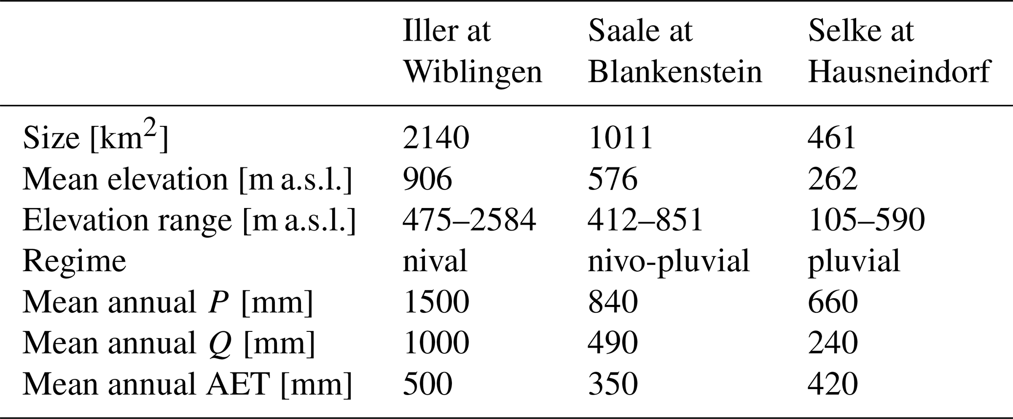
We selected three meso-scale catchments representing three different hydrologic regions of Germany: the Iller in the Alpine region, the Saale head water in the German low mountain range, and the Selke on the transition between the Harz mountains and the central German lowlands. This choice was made because we expect different processes to be more important in each of these catchments if we model them appropriately. For example, snow-related processes should be most important for the Iller catchment. Having these three example catchments allows us to have a closer look at the processes that can explain model performance and the learning capabilities of specific models focusing less on spatial diversity and more on investigating the information content within time series. The location of the catchments within Germany and their topography are shown in Fig. 1, and Table 1 provides some summary information for each catchment.
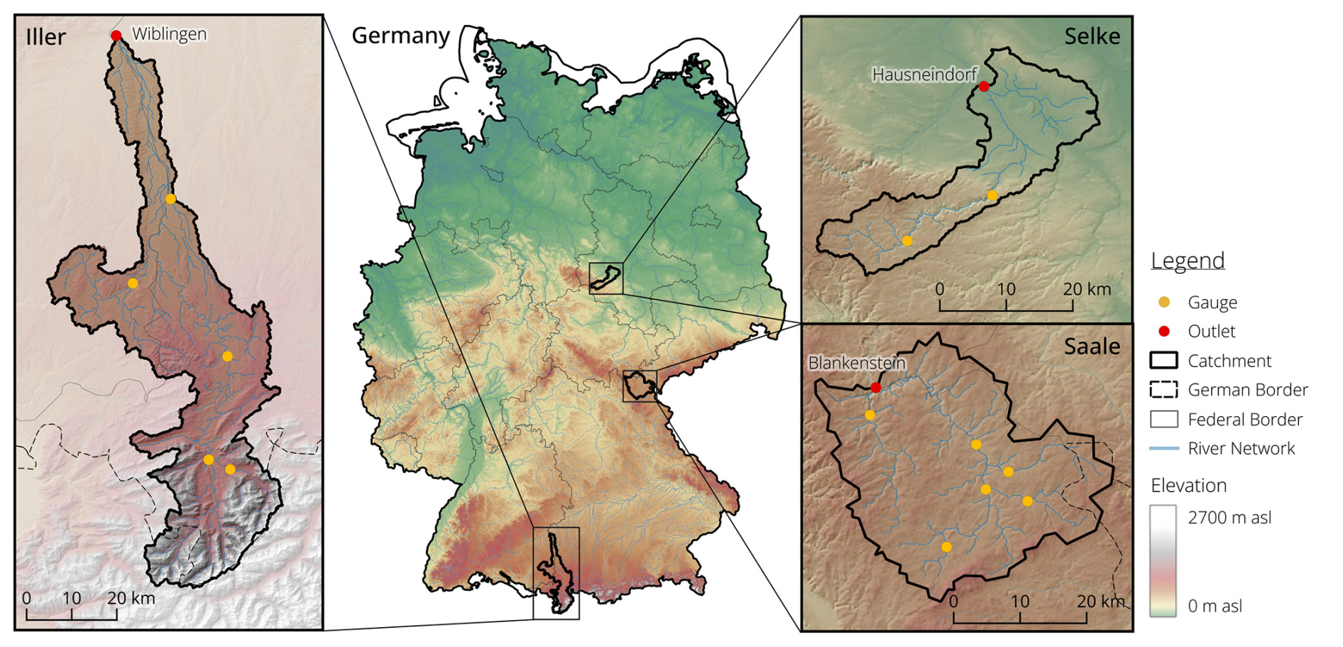
Figure 1Geographic location, topography, and gauging locations of the sub-basins of the study catchments.
Table 1Overview of the catchment characteristics for the three study catchments: Iller, Saale, and Selke. P= precipitation, Q= discharge, AET = actual evapotranspiration (P−Q).
2.1.1 Iller
The Iller catchment area up to gauge Wiblingen is 2140 km2 and has a diverse topography, including mountainous regions in the south with elevations above 2000 m a.s.l. and lower, flatter areas in the north. Approximately 50 % of the catchment area is cropland and pastures, about 30 % is covered by forests, predominantly mixed and coniferous forests, about 10 % is urban area, and about 10 % is covered by bare rock, sparsely vegetated areas, peat, and water bodies. A variety of soil types are found in the catchment, including lithosols and Cambisols (shallow, rocky, and well-drained), which predominate in the southern mountainous regions and cover about 25 % of the catchment. Cambisols (well-drained) occupy about 30 % of the catchment area and are found primarily in the mid-elevation regions. Alluvial soils (well-drained) are prevalent in the northern part of the catchment, along river valleys, and comprise about 20 % of the total area. Gleysols (poorly drained and often waterlogged) are found in wetter, low-lying areas and wetlands and comprise about 10 % of the catchment. The bedrock geology consists of Mesozoic limestone and dolomite in the Alpine region. North of the Alps, the bedrock transitions to the Molasse Basin, which consists of Tertiary sedimentary rocks, including sandstones, marls, and conglomerates. The northern plains are dominated by Quaternary alluvial deposits of gravel, sand, silt, and clay.
2.1.2 Saale
The catchment area of the Saale at gauge Blankenstein is 1011 km2 with a varied topography, where the upper regions are hilly to mountainous (elevations around 700–900 m a.s.l.) and the downstream areas have more gentle slopes. About 60 % of the catchment area is used for agriculture and pasture, about 30 % of the catchment area is covered by forests, mainly coniferous, and about 10 % is urban area (see also Guse et al., 2019). Podzols (well-drained) are prevalent in forested areas and cover about 20 % of the catchment. Cambisols (well-drained) cover about 30% of the catchment and are found in both agricultural and forested areas. Gleysols (poorly drained and often waterlogged) are found in wetter, low-lying areas and wetlands and cover about 10 % of the catchment. Loess soils (highly productive) and alluvial soils (well-drained) each cover about 20 % of the catchment. In the upper part of the catchment, the geology consists of metamorphic and igneous rocks (schists, gneisses, and granites). To the north, the geology changes to Triassic sedimentary rocks, including sandstones, marls, and limestones. Along the river valleys and floodplains, Quaternary alluvial deposits of gravel, sand, silt, and clay dominate.
2.1.3 Selke
The Selke catchment at gauge Hausneindorf covers 463 km2. The catchment has varied topography, with the upper regions being mountainous and more gentle slopes in the downstream areas. Approximately 55 % of the catchment area is used for agriculture, and about 35 % of the catchment is covered by forests, predominantly mixed and coniferous forests. Around 7 % is urban area, and about 3 % is covered by natural grasslands, wetlands, and water bodies. Podzols (well-drained) are prevalent in forested areas, covering about 25 % of the catchment. Cambisols (well-drained) cover around 30 % of the catchment and are found in both agricultural and forested areas. Gleysols (poor drainage and often waterlogged) are present in wetter, low-lying areas and wetlands, covering about 10 % of the catchment. Loess soils (highly productive) cover about 15 % of the catchment. Alluvial soils (well-drained) are found along river valleys, covering about 20 % of the area. Schist and clay stone are found in the mountain area, and Tertiary sediments with loess soil are found in the downstream areas. Highly permeable Quaternary alluvial deposits dominate along river valleys and floodplains.
2.2 Data
For each catchment, static catchment properties and dynamic data were collected. The static data comprise information about soils (horizon depth, sand and clay content), land use (classes from the CORINE map (CLMS, 2019) for SWAT+), and topography. The dynamic data comprise precipitation (P), air temperature (T), and estimated potential evapotranspiration (PET) in the form of gridded data, as well as discharge (Q) measured at the outlet of the catchment, and are available for the period 2000–2015. The available data and their temporal and spatial resolutions are summarized in Table 2.
Yamazaki et al. (2019)CLMS (2019)BGR (1999)Zink et al. (2017)Zink et al. (2017)Hargreaves and Samani (1985)Table 2Static and dynamic input data for each catchment. The dynamic input data (time series of precipitation, potential evapotranspiration, air temperature, and discharge) are available for the period 2000–2015.
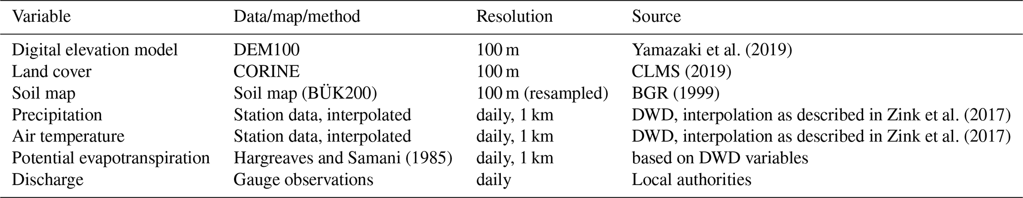
Gridded values for temperature and precipitation were obtained by interpolating the observations from meteorological stations. The density of stations used for interpolation varies over the years, but for our study catchments and period, it was between 20 and 30 stations per catchment. PET was estimated using the Hargreaves and Samani equation (Hargreaves and Samani, 1985), with minimum and maximum daily air temperatures from the meteorological stations and subsequent spatial interpolation. Details of the method can be found in Boeing et al. (2022). As some process-based models require station-based or lumped input data, weighted averages of the grid cell values contributing to individual sub-basins or hydrologic response units (HRUs) were generated.
2.3 Hydrological models
To address our research questions, we set up and applied three process-based and four data-driven hydrological models.
2.3.1 Process-based lumped and semi-distributed models
The process-based models are all provided with the same meteorological data (precipitation, temperature, and potential evapotranspiration) and linked with and run through the Python framework SPOTPY (Houska et al., 2015). SPOTPY allows for greater consistency between the runs of the different models, ensuring that all the sampling and input data are exactly the same.
GR4J
GR4J (Génie Rural à 4 paramètres Journalier) is a daily lumped rainfall-runoff model designed for hydrological simulation and streamflow forecasting (Perrin et al., 2003). The production store represents soil moisture processes, including infiltration and evaporation. The percolation and baseflow routine simulates groundwater contributions. The routing store manages the flow routing through the catchment. The flood routing itself is done using a unit hydrograph that accounts for the temporal distribution of the runoff. The model is parsimonious, requiring only four parameters, and has provided reliable results with minimal data requirements in the past (Smith et al., 2019; Kuana et al., 2024). The four parameters that are used in the standard model variant are as follows: maximum capacity of the production store (mm), groundwater exchange coefficient (mm d−1), 1-day-ahead maximum capacity of the routing store (mm), and time base of the unit hydrograph (d−1). To improve discharge modelling in catchments influenced by snow, GR4J is often combined with the CemaNeige snow module (Valéry et al., 2014), which comes with two additional parameters. In this paper, we used the GR4J and CemaNeige implementations that are provided through the Raven hydrological modelling framework, as they are perceived as exact emulations of the original models (Craig et al., 2020). The Raven GR4J implementation offers the possibility to run GR4J in a semi-distributed fashion. We used a sub-basin delineation for better input data representation. With only six parameters, this model is expected to perform well also under parsimonious calibration strategies. The parameter ranges used in this study are shown in Table S1 in the Supplement.
HBV
The HBV model is a semi-distributed model, i.e. a catchment can be divided into different elevation and vegetation zones as well as into different sub-basins. The model consists of several model routines and simulates catchment discharge based on time series of precipitation and air temperature and estimates of potential evaporation rates. We used it in the version HBV-light (Seibert and Vis, 2012) and divided the catchment only into elevation zones and sub-basins, not explicitly accounting for different land cover.
In the snow routine, snow accumulation and snowmelt are calculated using a degree-day method. Meltwater and precipitation are retained in the snow pack until they exceed a certain fraction of the water equivalent of the snow. Liquid water in the snow pack refreezes according to a refreezing coefficient. The soil routine simulates groundwater recharge and actual evaporation as a function of actual water storage. Actual evaporation from the soil box is either the potential evaporation or linearly reduced with decreasing soil moisture. In the response routine, discharge is calculated as a function of water storage. Groundwater recharge is added to the upper groundwater box and percolates from there to the lower groundwater box. Finally, a triangular weighting function is applied in the routing routine to simulate the routing of the runoff to the catchment outlet. When different elevation zones are used in the model, changes in precipitation and temperature with elevation are taken into account. HBV has a relatively small total number of model parameters, allowing the use of parsimonious calibration strategies. In our setup, we used 11 parameters to be calibrated plus 4 parameters that were fixed to default values. The parameter ranges used in this study are shown in Table S2.
SWAT+
The Soil Water Assessment Tool Plus (SWAT+) is a continuous, semi-distributed ecohydrological model. It is a restructured version of the original SWAT (Arnold et al., 1998; Bieger et al., 2017), designed to simulate the effects of land management and climate on hydrological processes and water quality. The catchment is divided into sub-basins that are further subdivided into HRUs that each represent a unique combination of land use, soil type, and topographic conditions within a sub-basin. Soil water content is continuously updated based on the balance of incoming water (precipitation and irrigation) and outgoing water (evapotranspiration, runoff, lateral flow, and percolation) for each HRU. The Curve Number method is used to divide precipitation into surface runoff and infiltration. Actual evapotranspiration is calculated based on water storage in soil, plant characteristics, and open water bodies. Percolation is simulated by tracking the movement of water from the root zone to deeper soil layers and eventually to groundwater. Percolation rates depend on soil properties, soil moisture levels, and the amount of water available after accounting for evapotranspiration and surface runoff. Groundwater flow is routed through user-defined aquifers and contributes to discharge based on storage and retention parameters. SWAT+ allows the calibration of a large number of parameters, leading to considerable model flexibility, but therefore usually requires less parsimonious calibration strategies and a higher degree of user knowledge.
An overview of the different resolutions and aggregations of the input data for the process-based models is given in Table 3, and the parameter ranges used in this study are shown in Table S3.
2.3.2 Data-driven models
We selected four data-driven models with the aim of covering a wide range of model complexity, from very simple ones (EDDIS and RTREE), which serve as a lower benchmark, to simple approaches based on neural networks (ANN) and to the current state of the art (LSTM), which serves as an upper benchmark. Details of each model are described below. Many other data-based methods have been used for modelling hydrological systems, e.g. NARX networks (Renteria-Mena et al., 2023) or random forests (Schoppa et al., 2020). These typically show performances between our lower and upper benchmarks; therefore, we did not include them in the study for the sake of brevity.
Empirical discrete distributions (EDDIS)
This approach represents the case where there is no prior knowledge of the structure of the real-world system, and therefore the model can learn only from the available training data. The model is deliberately kept as simple as possible to serve as a lower benchmark and consists of the multivariate joint discrete (binned) distribution of all available training data, including the desired model output (here, discharge). The binning method is explained in Sect. 2.4. As the model is built directly from the training data, no training is required. Applying the model consists of binning a given set of input data and then retrieving the conditional discrete distribution of the output given the input from the joint distribution. If necessary, this probabilistic prediction can be reduced to a single number by calculating the expected value. The model can be interpreted as a probabilistic lookup table or analogue model, and for applications where no analogue situation was included in the training data, we set the model prediction to be a uniform – i.e. minimally informative – distribution of the output value. By design, the model cannot account for memory effects, such as those caused by water storage in the catchment. The only way such memory effects can enter the prediction is through the model input. We therefore built several models with different sets of predictors, including those with temporal aggregations, and then selected the set of predictors that had the best predictive performance across all catchments. Notably, this is not necessarily the case for the predictor set with the largest number of variables, as overfitting quickly occurs in such cases. We tested all possible combinations of the following options: splitting the range of values of each variable into 2, 4, 6, or 8 bins; providing precipitation input either spatially lumped or split into two sub-basins; providing precipitation input either as a single variable with the value of the current day or as four variables, i.e. daily value of the current day and day −1, precipitation sum of day −2 through −6, and precipitation sum of day −7 through day −30, thus providing precipitation memory; and providing spatially lumped temperature as a single variable with the value of the current day or as two variables, i.e. daily value of the current day and mean temperature of day −1 through day −30, thus providing temperature memory. Among all variants and across all catchments, the best input combination was the spatially lumped combination of precipitation and temperature, both with memory (preceding day and preceding week), splitting the value ranges into two bins each. This model was used for all further investigations.
Regression tree (RTREE)
Like the EDDIS model, regression trees are simple and completely agnostic to the structure of the real-world system, so their predictive power depends entirely on the information content of the chosen input data. The RTREE therefore also serves as a lower model benchmark, but it is slightly more sophisticated than EDDIS: through supervised learning, it optimizes the partitioning of the input data to maximize the predictive power of the output. We used the “fitrtree” function in MATLAB R2024a to fit the trees, testing the same input variants as for EDDIS. Interestingly, the same spatially lumped precipitation–temperature input set with memory as for EDDIS showed the best performance and was therefore used for all further studies. Regression trees have been applied to hydrological problems, e.g., by Zhang et al. (2018); Paez-Trujilo et al. (2023).
Artificial neural network (ANN)
The ANN consists of multiple layers of interconnected nodes or neurons, including input, hidden, and output layers. Each neuron in the hidden layer applies a weighted transformation to the input data, followed by a nonlinear activation function to capture nonlinear relationships. During training, the model adjusts its weights using backpropagation, an optimization algorithm designed to minimize the error between predicted and observed outputs. This allows the model to learn from the data and improve its predictions over time. In hydrological modelling, ANNs are used because of their ability to capture complex, nonlinear relationships between variables (Hsu et al., 1995). However, because an ANN lacks inherent memory or recurrence, it cannot alone account for temporal dependencies in hydrological data. To account for the strong autocorrelation typically present in such data, it is necessary to shift the inputs over a time window. By applying a time window lag, the ANN can account for delayed effects, i.e. inputs from previous time steps are used to predict current conditions. In this case, the ANN is used to predict discharge based on past time series data, including variables such as precipitation, temperature, and evapotranspiration. The input data are shifted by seven daily time steps, generating 21 input features. The model architecture consists of three layers of 64 hidden units each. The first two layers use a rectified linear unit activation function. The training optimization includes a learning rate of 0.001, which decays by a factor of 0.5 after every 5 epochs. A 40 % dropout rate is applied to prevent overfitting. The model is trained for 30 epochs with a batch size of 32. To account for variability due to random weight initialization, each model is initialized and trained three times.
Long short-term memory (LSTM) network
Long short-term memory (LSTM) networks have become the benchmark model for streamflow and rainfall-runoff modelling (Kratzert et al., 2018; Acuña Espinoza et al., 2024). Unlike ANNs, which inherently cannot capture temporal dependencies, LSTM networks are specifically designed to handle time-series data through their internal memory cells and gating mechanisms. In this study, three LSTM networks are built for each of the three test catchments. The model architecture consists of an LSTM layer, followed by a linear output layer, both featuring 64 hidden units. The networks are trained with a learning rate of 0.01, and a learning rate decay factor of 0.5 is applied after every 5 epochs to optimize training. A 40 % dropout rate is used to prevent overfitting. Training is performed over 20 epochs with a sequence length of 365 d, and the forget gate bias is set to 1 to facilitate the learning of long-term dependencies. The LSTM networks predict discharge using the same input features as the ANN models, including precipitation, temperature, and evapotranspiration. However, unlike ANNs, the inputs are not shifted over time. To account for variability due to random weight initialization, each LSTM model is initialized and trained three times, and we use the average of the three models in any further analysis.
2.3.3 Data used by the models
All models are provided with the same meteorological forcing data and the daily discharge observations at the outlet of each catchment. Although the meteorological data were provided to each model as the same daily grid, different aggregations were applied to use the data. SWAT+ uses averages of the internally generated sub-basins and HBV, and the GR4J models use sub-basin averages delineated at the gauging stations (Table 3). EDDIS and RTREE use catchment-averaged data, and ANN and LSTM use sub-basin averaged data, all of them with several temporal aggregations (details are explained in the respective sections above).
Table 3Input data and temporal and spatial discretization of the data as used in the process-based and data-driven models. All of the data are daily. DEM = digital elevation model, PET = potential evapotranspiration.
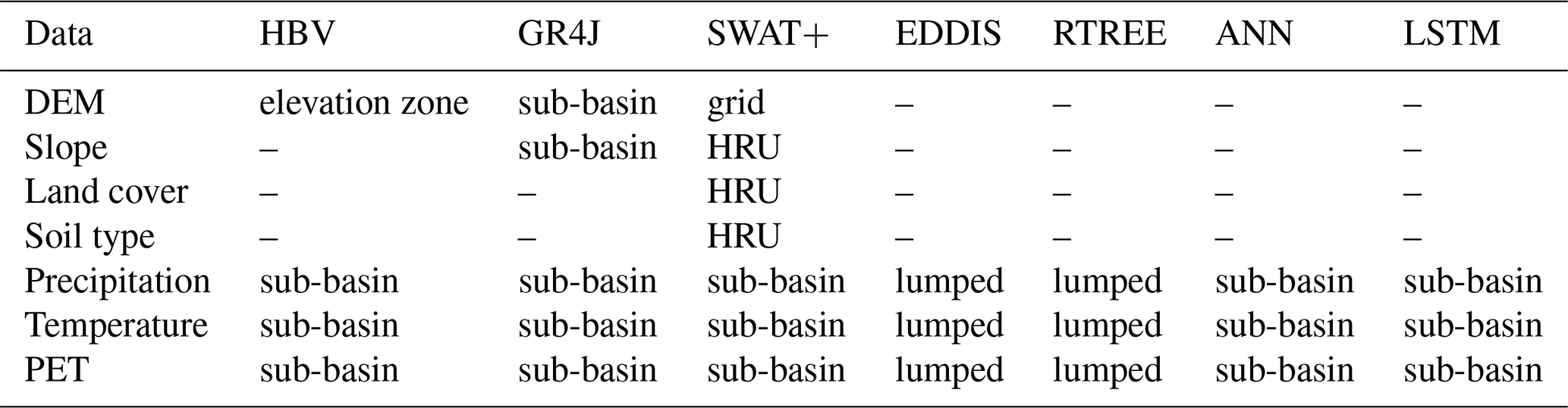
Some of the process-based models require additional data for the setup, which allow building the specific model architecture and partly also the model parameterization. For example, SWAT+ uses soil information and land use to define soil storage and root depth (Table 3). These additional data also require different spatial discretization, e.g. for SWAT+ to the HRU. For this study, these additional data are considered as part of the model structure and not as comparable input data, i.e. we treat these additional data as model-specific prior knowledge that constitutes the model architecture. EDDIS, RTREE, ANN, and LSTM do not apply additional static data.
2.4 Distance measures and objective functions
In this section, we describe the distance measures used to address research questions (Q1)–(Q4), specifically for data-driven catchment characterization, for model parameter estimation during model training, and for model performance evaluation.
In particular, for the characterization of catchments based on available data, we needed a measure that would allow the integration of multivariate data of different dimensions on a single scale, the measurement of the total variability of catchment dynamics both with and without memory, and the direct comparison of joint unconditional variability of all variables with conditional variability of the target variable, i.e. discharge, given all other variables. All of these requirements are met by joint entropy Hj, which is an information measure, as it operates on probabilities of variable values rather than on the values themselves. A good general introduction to information theory is provided by Cover and Thomas (2006), an overview of applications in the earth sciences by Kumar and Gupta (2020), and a comparison to other methods of uncertainty quantification by Abhinav and Rao (2023). Recent applications of information concepts to hydrology include, among others, Jiang et al. (2024a) for model training, Ehret and Dey (2023) for system classification, Moges et al. (2022) for data analysis, Azmi et al. (2021) for model evaluation, Ruddell et al. (2019) for model diagnostics, Neuper and Ehret (2019) for hydrometeorological data-driven modelling, and Nearing et al. (2018) for process diagnostics.
Information measures exist for both continuous and discrete distributions. Computing continuous information measures typically requires fitting a continuous parametric distribution function to the data, which can be challenging, especially for high-dimensional distributions and sparse data. Computing discrete information measures from continuous data requires binning, which inevitably leads to information loss, but is straightforward even for high-dimensional and sparse data. Because a central question of this paper is how well models learn from a small amount of data, we explain discrete information measures below and use them throughout the study.
For a multivariate set of discrete variables , and realization thereof , their overall joint variability can be measured by the entropy of their joint distribution Hj (j here indicates “joint”) according to Eq. (1).
If the log of the probability p is taken to base 2, Hj is measured in bits and can intuitively be interpreted as the number of binary (Yes/No) questions that would need to be asked to correctly guess a particular multivariate measurement if the joint distribution were known. Entropy therefore is a measure of uncertainty expressed as number of questions. Hj is non-parametric, seamlessly expands from uni- to multivariate datasets, and is therefore well-suited for our task. Additionally, lower and upper bounds of Hj exist. This allows standardization of results and thus facilitates inter-comparison between datasets of different dimensionality. The lower bound of 0 is reached by a Dirac distribution, and the upper bound of log2(n) is reached by a uniform distribution, where n is the number of bins.
While Hj measures the unconditional overall variability of a dataset, to evaluate model performance, we need to measure how uncertain we are about the value of the target variable of interest, knowing the model prediction. This is measured by conditional entropy Hc, where c indicates “conditional”, as shown in Eq. (2), where Y is the observed target value, y is a realization thereof, and X is the related model prediction.
For simplicity, Eq. (2) is shown for the case of a single target variable and a single prediction thereof, but Hc, like Hj, expands seamlessly to multivariate targets and predictions, and like Hj, it is bounded. The lower bound is 0, which is reached when the model unambiguously identifies the target observation, and the upper bound is the unconditional entropy of the target Hj(Y), which is reached when the model has no predictive power at all.
As mentioned above, binning of continuous data inevitably loses the information about the position of each variable value within the bin, and the fewer and wider the bins, the higher the loss. On the other hand, choosing many narrow bins leads to sparsely populated and hence non-robust distributions, especially for high-dimensional datasets. Binning therefore is a two-sided optimization problem. We solved it by choosing, for a given number of bins, their edge positions such that they (i) cover the entire value range of the data and (ii) minimize the sum of squared errors (SSE) between the original and the binned data, where the latter is represented by the respective bin centre. Such an optimization is essentially a clustering problem with SSE as the measure for the within-cluster distance, and we implemented it with the “clusterdata” function in MATLAB R2024a. Such a binning by optimization respects both the values and the frequency of the data. Regarding the choice of the number of clusters: for the predictors in the EDDIS model, we tested several options ranging from two to eight (see related paragraph above); for the observations and predictions of the target variable discharge then, we chose 12 as the best trade-off between resolution and bin population.
In summary, we used joint entropy and conditional entropy for data-driven catchment characterization (Q3). For performance evaluation of all models in (Q1), (Q2), and (Q4), we used the conditional entropy of the observed discharge given the simulated discharge. Additionally, we provide performance results measured by the Kling–Gupta efficiency (KGE) (Gupta et al., 2009) in the Appendix, as it is widely used in hydrology and thus facilitates the interpretation of results for hydrologists. In the Appendix, we also provide a table (Table A1) with a comparison of the characteristics of information-based and value-based distance measures. Several measures were used for model training. The reason for this is that the models used in this study cover a wide range from data to process based, and different training methods and appropriate performance measures are used in the respective communities. In order not to disrupt well-established method–measure interactions, we decided to keep the domain-specific measures, acknowledging the slight inconsistency we introduced. In particular, for all process-based models, KGE was used as an objective function during training; for RTREE, the root mean square error (RMSE) was used, and for ANN and LSTM, the mean squared error (MSE) was used. EDDIS did not require any training.
In order to better emphasize how well a particular model can learn from data of a particular catchment, we introduce a standardized measure of “relative learning” Lrel, as shown in Eq. (3):
where Lm is the learning of the model, defined as the difference between the conditional entropy of the model prediction when the training sample size is minimal and the conditional entropy of the model prediction when the training sample size is maximal. Llower and Lupper serve as upper and lower benchmarks for standardization, inspired by the general benchmarking suggestion of Seibert (2001). Llower is the smallest possible value Lm can take (here, 0), and Lupper, the largest (here, the unconditional entropy of the observed discharge of each catchment). Lm thus takes values between minus infinity and 1, where negative values indicate that the final performance is less than the lower benchmark, 0 indicates that a model cannot learn anything from the available data, and 1 indicates that a model can learn all information contained in the available data and perfectly predict the target.
2.5 Experiments
For all experiments (see overview in Table 4), training is done for each sample size, each replicate, each process-based model, and each catchment using Latin Hypercube Sampling (LHS). For details on the LHS settings, see the Supplement. All models, i.e. data-driven and process-based, have a warm-up run in the period from 1 January 2000 to 31 December 2000, and all training samples are from the period 1 January 2001 to 31 December 2010. Model performance was validated using an independent period from 1 January 2012 to 31 December 2015, also preceded by a warm-up period from 1 January 2011 to 31 December 2011. The simulations from this validation period are the basis for all presented model performances and model learning behaviour. Both training and test data periods were very similar in terms of the distribution of high and low flows. For all experiments (again, see overview in Table 4), we provide the models with 10 sample sizes from the available discharge data up to the full length of the time series. These are 2, 10, 50, 100, 250, 500, 1000, 2000, 3000, and 3654. For each sample size, the models are trained/calibrated on discharge, and only the data of the specific sample size were evaluated during the training. The parameter ranges that were defined for each model can be found in the Supplement.
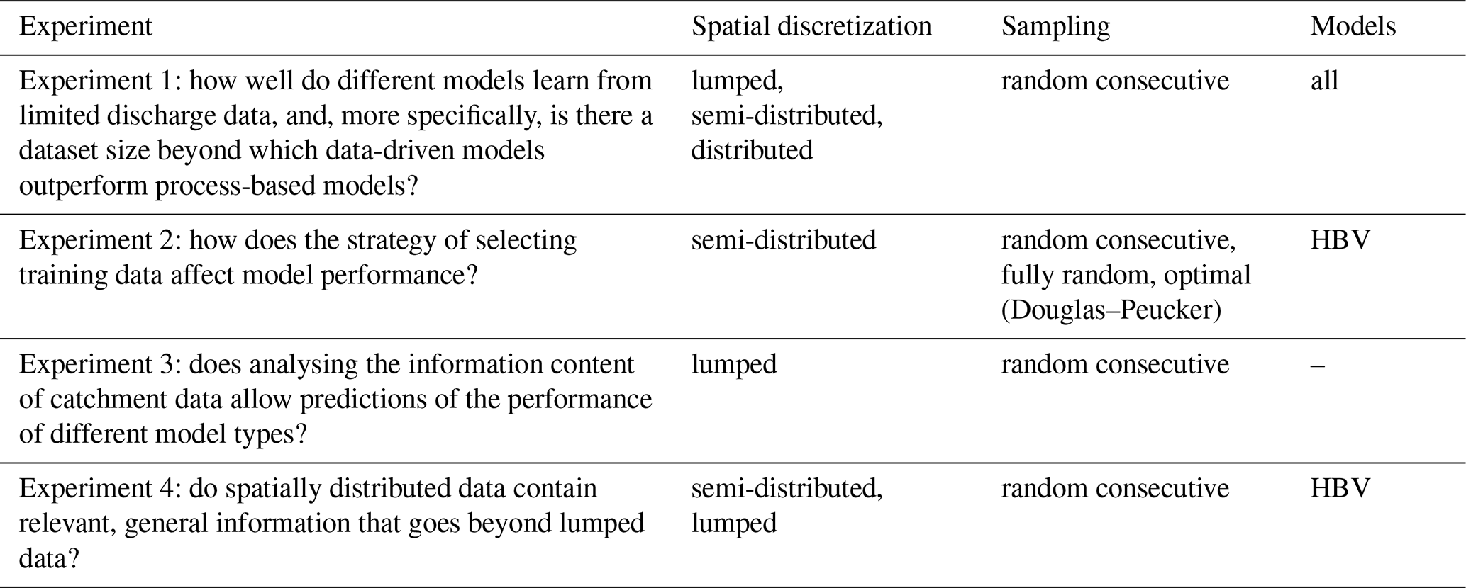
Table 4Overview of the model experiments, purpose, and models used. “semi-distributed” means the spatial distribution that is commonly used for each model, i.e. for the HBV model divided into sub-basins and for SWAT+ divided into HRUs.
For the different experiments, we used various sampling schemes (Fig. 2): in the fully random sampling scheme, we sampled x random points that form the basis for calculating the model performance, with x being the respective sample size. For each sample size, we performed 30 repetitions, i.e. 30 random samples over the training period. For the random consecutive sampling scheme, we randomly sampled a single point in the time series and then used all the subsequent points. If the sample size was larger than from that point to the end of the data, the points preceding the single sampling point were also used to achieve the desired sample size. For each sample size, we used 30 repetitions, i.e. we sampled a random starting point of the continuous series 30 times. This sampling scheme resembles the case where a measurement campaign is started (randomly in time) and continues until the study or funding ends. This is probably the most common type of dataset we have available for model training, and it neglects potentially interesting periods, such as floods or long dry spells leading to droughts.
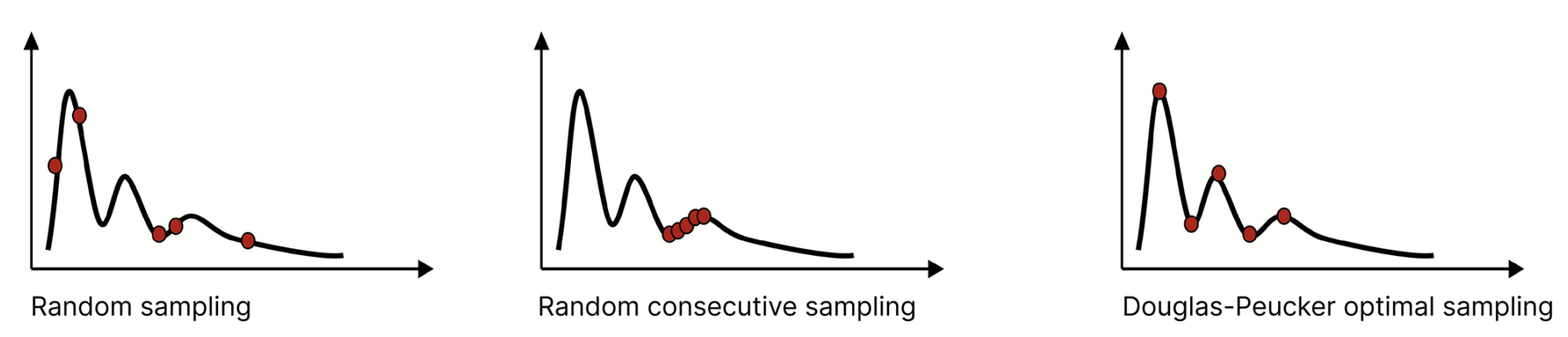
Figure 2Sketch of the different sampling strategies, i.e. fully random, random consecutive, and optimal sampling using the Douglas–Peucker algorithm.
In order to achieve optimal sampling, the algorithm proposed by Douglas and Peucker (Ramer, 1972; Douglas and Peucker, 1973) was selected. The algorithm searches for the most informative points, specifically targeting turning points such as flood peaks, points before the start of the rising limb of the hydrograph, and so forth. The most informative points for this algorithm are those where there are changes in the time series. This approach could be used if we did training but wanted to reduce the dimension/data size for one reason or another. An example of the points selected using the Douglas–Peucker algorithm is shown in the supplementary material for some of the used sample sizes of the Iller catchment (Fig. S1).
2.5.1 Experiment 1: how well do different models learn from limited discharge data, and, more specifically, is there a dataset size beyond which data-driven models outperform process-based models?
In this main experiment, we compared the learning behaviour of three process-based and four data-driven models. We trained all models with data from the same time period using the random consecutive sampling scheme, providing each model with the same increasing sample and the same 30 repetitions of each sample size to train. Although the exact same gridded data were provided to each model, different pre-processing was required to force the models. For the semi-distributed process-based models, the data were spatially aggregated to sub-catchments (HBV model, GR4J, SWAT+), and for the simpler data-driven models (EDDIS, RTREE), the data were fully lumped. By comparing the conditional entropy of each model for the independent validation period, we can assess how well the models learn relative to each other and how this varies between the different catchments for which the experiment is conducted.
2.5.2 Experiment 2: how does the strategy of selecting training data affect model performance?
In this experiment, we tested the effect of different sampling schemes on the performance of the HBV model. To assess the influence of the training data on the actual training, we tested three sampling schemes: fully random sampling, consecutive random sampling, and optimal sampling using the Douglas–Peucker algorithm. As an example of a model commonly used in a lumped or semi-distributed model setup, this experiment was performed using the HBV model.
2.5.3 Experiment 3: is there a relationship between the information contained in the data and the shape of the learning curve for different models that allows predicting the achievable model performance?
Concepts from information theory have been used for a broad range of tasks related to data retrieval and system analysis. For example, Foroozand and Weijs (2021) used them for the optimal design of monitoring networks, Neuper and Ehret (2019) to identify the most important predictors for quantitative precipitation estimation, and Sippel et al. (2016) for a data-based dynamical system analysis. Along the same line, we used information concepts here to determine whether we can predict the success of training a model from a prior analysis of the available multivariate input and target data (precipitation, temperature, evapotranspiration, streamflow). Specifically, we investigated whether model performance, expressed as the conditional entropy of the streamflow given the input data, can be predicted from the joint entropy of the input and target data. These two types of entropy give different insights: joint entropy – about the overall variability (information content) of the data; conditional entropy – about the information content of the input data about the target data.
We computed the unconditional entropy of the datasets with four variables (input P, T, PET, and target Q) with and without memory, i.e. with and without any temporal dependence of the data: (1) only the value at time step t is used, resulting in four variables (P,T, PET, Q); (2) in addition to the four variables at time step t, the variables at time step t−1 are also used, resulting in eight variables that are each binned; (3) in addition to the four variables at time step t, the variables averaged over the preceding week t−1 to t−6 are used, resulting in eight variables that are each binned. The joint entropy values between cases (2) and (3) can be directly compared, as the base in both cases comprises eight variables, each in eight bins. Instead, the values of (1), which does not take into account any memory, cannot be directly compared to those of (2) and (3), as the base includes only four variables, each in eight bins (Table 5).
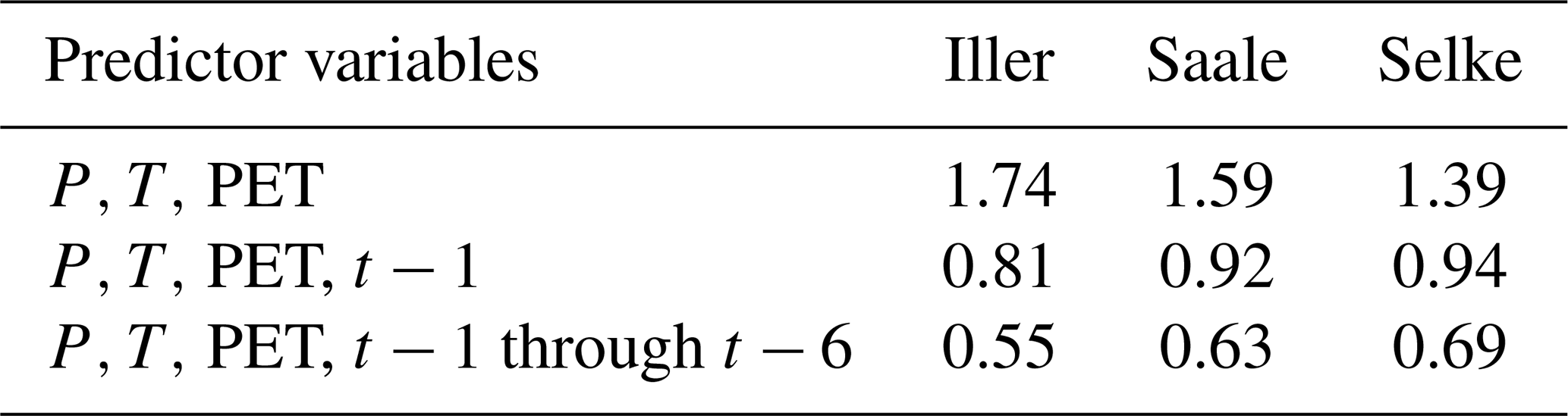
We computed the conditional entropy of the input data with respect to the target variable discharge Q at t0 based on the three predictor variables P, T, and PET without memory, i.e. also at t0. Again, we looked at the three cases: (1) three predictors, and no time aspect is considered at all; (2) three predictors, and for each variable, also the value of the preceding day; (3) three predictors, and for each variable, also the average value of the preceding week (Table 6). Here, for all three cases, the conditional entropy values can be directly compared with each other, as here the target (streamflow) was binned into eight bins for each analysis. The maximum entropy value for these cases is 3 (= log2(8)).
2.5.4 Experiment 4: do spatially distributed data contain relevant, general information that goes beyond lumped data?
To test the benefit of more spatial distribution in the input data for model training, we used the HBV model and set it up for each catchment in both a lumped and a semi-distributed manner by using sub-catchments. Both model versions were trained using the same time periods and the consecutive random sampling scheme, but the lumped model received catchment areal averages of precipitation, temperature, and evapotranspiration, whereas the semi-distributed models received these meteorological inputs averaged to the sub-catchments.
3.1 Experiment 1: how well do different models learn from limited discharge data, and, more specifically, is there a dataset size beyond which data-driven models outperform process-based models?
From this experiment, we were able to generate learning curves for each model and each catchment. The learning curves show how much a model has learnt with increasing sample size during training. This means that if the conditional entropy, Hc, decreases with increasing sample size, the models are learning from more discharge data. The band around the median learning curve indicates both the effect of different replicated samples at each sample size and the calibration uncertainty.
For all catchments, we found a grouping of the process-based models and the data-driven models where the data-driven models learn longer than the process-based models but the process-based models start with lower conditional entropy values than the data-driven models. However, this is expressed to different degrees for each of the three catchments.
The learning curve for the Iller catchment (Fig. 3, left panel) shows that, for all models, the conditional entropy decreases with increasing sample size, Hc, i.e. they learn with increasing training sample size. This is true for all models, both data-driven and process-based. The process-based models start with lower conditional entropy values (between 2.3 and 1.8) when provided with very small sample sizes than the data-driven models (Hc 2.1 to 2.6). The process-based models learn with increasing sample size and reach a learning plateau at around 500 samples. The data-driven models continue to learn with increasing sample size, and the LSTM in particular outperforms all the process-based models. The ANN also continues to learn and reaches performances that are comparable to some of the process-based models. The simple data-driven models (EDDIS and RTREE) have a steep learning curve at the beginning and, based on the conditional entropy value, almost reach the performance of the process-based model SWAT+. However, compared to the LSTM, their learning is much slower after a sample size of 500.
For the Saale catchment (Fig. 3, middle panel), there is a similar grouping of process-based versus data-driven models. Again, the process-based models start their learning curve at lower conditional entropy values than the data-driven models and soon reach a plateau with a relatively small sample size. The data-driven models have a very steep learning curve at the beginning and continue to learn slowly, but they do not reach conditional entropy values as low as those seen in the Iller catchment, nor do they reach the performance of the process-based models. Three models of the model groups stand out. Among the process-based models, the SWAT+ model has a lower performance at the beginning of the learning curve, i.e. when it is provided with a small sample for training, and its performance remains below that of the other process-based models until the end of the learning curve, i.e. when it is provided with all the data available for training. The ANN model starts with a rather high performance compared to the other data-driven models and stays in a similar arrangement to the learning curve of the process-based models. The LSTM, as already seen for the Iller catchment, has the steepest learning curve and continues to learn after all other models have finished. For the Saale catchment, the learning curves are quite different from those of the Iller catchment, and all models, process-based and data-driven, except for the LSTM model, plateau after a sample size of 500 to 1000. This catchment shows an intermediate data variability and an intermediate learnability from the ranking of the joint entropy of the input data and the ranking of the conditional entropy.
For the Selke catchment (Fig. 3, right panel), there is a relatively wide spread between the learning curves of the process-based models, with the simplest models GR4J and HBV starting and reaching the highest performance, although the overall learning curve is rather flat. The SWAT+ model starts with a similar performance but essentially shows no learning as sample sizes increase above 500. The performance of the simple data-driven models (EDDIS and RTREE) and ANN is very similar to that of the SWAT+ model. The simple data-driven models start their learning curve with very low performance, learn quickly with increasing sample size, and stop learning at a sample size of 1000. The ANN model continues to learn but with a very flat learning curve. The LSTM, like for the other two catchments, knows very little at the beginning, then has a steep learning curve and continues to learn. Unlike for the Iller and Saale catchments, the LSTM does not outperform the process-based models HBV and GR4J.
If we compare only the relative learning (Fig. 4), i.e. how much a model learns without considering the initial performance, but only compare the performance at the beginning and at the end of the learning curve, then we see that the data-driven models learn the most, with the LSTM model clearly outperforming all other models. The LSTM model may outperform the other data-driven models due to its ability to flexibly capture short- and long-term dependencies, which are essential for modelling hydrological processes. For this consecutive sampling scheme, the HBV model also shows a learning capability comparable to the ANN and RTREE. However, it should be noted that it does so mainly in the first sample size increase and then plateaus (Fig. 3). For our comparison, the SWAT+ model has a lower learning capability, and for the GR4J model, the learning capability varies with the catchment in which it has to learn.
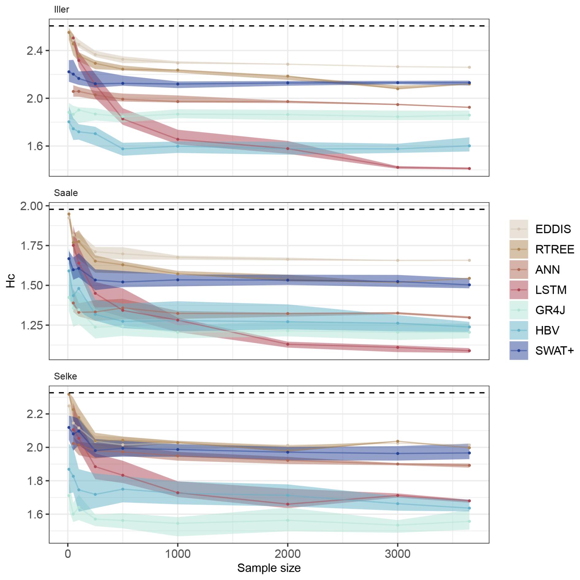
Figure 3Learning curve using the continuous random sampling strategy for the different models and catchments, showing the changes in the conditional entropy Hc with increasing sample size. The lower the values of Hc, the more the model could learn from the data (i.e. the better the discharge simulations are). The band of the learning curves represents the 25th to 75th percentile of the ensemble of 30 repetitions, and the line is the median. The dashed line shows the maximum possible entropy, which can be used as a benchmark, in a similar way to how the mean discharge prediction is used in the Nash–Sutcliffe efficiency. Note that for visibility reasons, we applied a different y-axis scaling for each catchment. The samples are independent from each other, and the lines are there only for visualization.
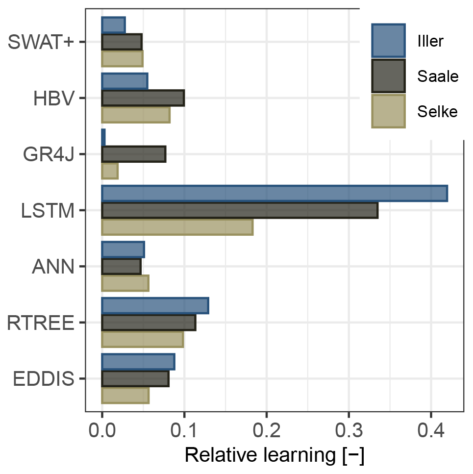
Figure 4Relative learning of the different models using the continuous random sampling scheme. Relative learning is defined as the difference between the beginning and the end of the learning curve (Eq. 3).
It is well known that discharge is much easier to model in some catchments than in others, either because of a pronounced seasonality in discharge, expressed as spring flood, summer low flow, or the like, or because the catchment response is very similar to the precipitation that falls on the area – or even because there may be errors both in the forcing meteorological data and in the data used for evaluation – in our case, discharge. These errors can be so large that, as a consequence, the preservation of mass (inscribed in process-based models but not for data-driven models) is violated, and the water balance is not closed. What is interesting, however, is how differently the process-based models we used in our study were able to simulate and learn the discharge with the same input data. For example, the Iller catchment, which had high variability but also high learnability from the data alone, has a high spread of the learning curves of the individual models, indicating that the model architecture of some of the process-based models is somehow more advantageous than the model architecture of others for the training of this catchment. The Iller catchment could be modelled well and learnt well (up to the learning plateau) by the rather simple process-based models GR4J and HBV, but with generally worse model performance for the spatially higher-resolved SWAT+ model.
The strongest learning performance was observed for all data-driven models, with the LSTM showing the steepest learning curve and ultimately achieving the highest predictive accuracy once a sample size of 2000 was reached. Unlike simpler data-driven models (e.g. EDDIS and RTREE), both the ANN and LSTM models used semi-distributed input data. It is likely that the LSTM benefited from this input by discovering complex relationships that the simpler models could not. While the discretization of the input data does not explain why the LSTM continues to learn when the ANN stops, this behaviour can be attributed to the model architecture itself. The LSTM, similar to a classical hydrological model, essentially operates as a state space model. We refer to this inherent architectural advantage as an inductive bias: unlike standard ANNs, which lack memory cells and intrinsic recurrence, the design of the LSTM (De la Fuente et al., 2024) allows it to continuously integrate new information over time, enabling persistent learning and improved performance.
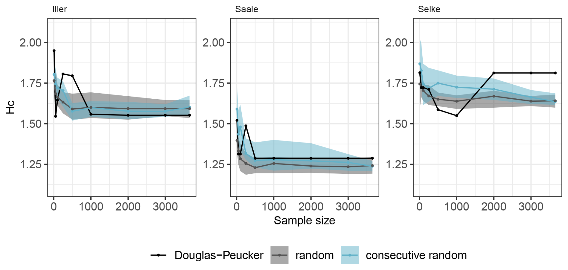
Figure 5Learning curve using the different sampling schemes for the HBV model, showing the changes in the conditional entropy Hc with increasing sample size. The lower the values of Hc, the more the model could learn from the data (i.e. the better the discharge simulations are). The band of the learning curves represents the 25th to 75th percentile of the ensemble of 30 repetitions, and the line is the median. The samples are independent from each other, and the lines are there only for visualization.
3.2 Experiment 2: how does the choice of training data, i.e. the information content in a given dataset, affect training for a specific problem?
The different sampling strategies have been investigated only for the HBV model. Here, the learning curves for the Iller catchment (Fig. 5) show how different sampling compositions affect learning. We have a band around the consecutive random and the fully random sampling because we did 30 repetitions of the random sampling but only one line for the learning curve of the Douglas–Peucker sampling because this algorithm gave us only the most interesting points, presumably the optimal sampling. Notably, the learning curves of the random and consecutive random sampling strategies look very similar. For these two, the HBV model learns more for the Iller and Saale catchments than for the Selke catchment: when expressing learning as the difference in conditional entropy between the smallest and the largest sample divided by the conditional entropy of the smallest sample, then learning reduced the conditional entropy by 10.3 % for the Iller, by 16.6 % for the Saale, and by only 9.1 % for the Selke catchments (values are averages of the random and consecutive random approach). The Douglas–Peucker learning curve appears to be much jumpier than the learning curves of the full random and the consecutive random learning curves. It should be noted that the learning curves for both random sampling schemes show the median of 30 replicates and the 25th and 75th percentiles, smoothing out the behaviour of the individual lines used to calculate these statistics. Each of these individual repetition lines could (and some do) have jumpy behaviour similar to the Douglas–Peucker curve.
The learning curve using the Douglas–Peucker sampling starts with the highest conditional entropy for the Iller catchment but the lowest conditional entropy for the Saale and Selke catchments compared to the other two sampling strategies. The largest samples show exactly the same entropy value in the learning curves, starting for the Iller catchment with a sample size of 1000, for the Saale catchment with a sample size of 500, and for the Selke catchment with a sample size of 2000. These same entropy values are derived from the selection of exactly the same model for these sample sizes, i.e. there is no further learning with the additional points that increase the sample size.
When using the consecutive random sampling scheme, the HBV model learns approximately up to a sample size of 1000 and then reaches the plateau of the learning curve. The fully random sampling scheme gave the best performance, i.e. the lowest conditional entropy, compared to the others at the beginning of the learning curve and also plateaus around a sample size of 500. The learning curves for Iller and Saale look very similar at the end for all sampling schemes, and there is no significant difference visible in model performance in terms of conditional entropy. For the Selke catchment, the conditional entropy of the Douglas–Peucker sampling is higher than for the two random sampling strategies, which can be explained by the additional points in the larger samples provided for training. These additional points come from turning points before the rising limb and contain more low flow values. Optimization focusing both on low and high flow (first selected by the algorithm) then attempts to optimize for both flow aspects, and the overall model performance is reduced. Using a different training setup that increases the sample size of the LHS, or using a different training algorithm such as the dynamically dimensioned search (Tolson et al., 2009), could help avoid this worsening in the learning curve (Fig. S1). Using the KGE instead of the conditional entropy for the learning curve does not yield such a decrease to lower performance in the Selke catchment and shows smoother learning (Fig. S1). Because we included only the HBV model in this side experiment to test different sampling schemes, we cannot make a general statement. However, with relatively small sample sizes between 500 and 1000 d, the model has already learnt to its maximum. Similar ranges were also found in Brath et al. (2004), Melsen et al. (2014), and Sun et al. (2017). For the catchments we used in this study, all of which are in a humid climate, it does not seem to matter whether the sample is made up of a continuous time series of discharge or a random sample over many years, suggesting that these sample sizes sufficiently represent the natural variability in flows and hydrologically active periods.
With the resulting learning curves when using random consecutive sampling, we can infer how long such a measurement campaign should last in a given catchment to capture enough information for the model to learn. This is different for each catchment but somewhere between 500 and 2000 points, and comparing the variability inherent in the data that we could quantify using the joint entropy, the conditional entropy of the discharge using these variables as predictors, and the learning curves themselves can provide useful guidance.
The other two sampling schemes we tested are the fully random scheme and the optimal scheme using the Douglas–Peucker algorithm. These sampling strategies are more commonly used in practice during event-based sampling campaigns or when there are large datasets and only a representative or essential information is sampled to reduce computational efforts for model training. We found that fully random sampling slightly outperformed Douglas–Peucker sampling, despite the idea that this algorithm would provide the model with optimal sampling points for training. This was particularly true for the Selke catchment, where the learning, expressed as a reduction in conditional entropy, was reversed because additional points in the sample realigned the model focus away from mainly floods to also low flows, and the parameter search ended in exactly the same model for all samples larger than a catchment-specific sample size. A major advantage of random sampling over optimal sampling is the ability to repeat the sampling, which ultimately provides learning curves from statistics that can be used as a guide, rather than overthinking why one increase in sample size did not produce the expected learning while the next did.
3.3 Experiment 3: is there a relationship between the information contained in the data and the shape of the learning curve for different models that allows predicting the achievable model performance?
In this experiment, we focused on the information content of the input data about the target (streamflow) by measuring the entropy of the conditional distribution of the target given the input data. This is equivalent to the EDDIS model, which essentially constitutes a purely data-driven model with almost no added model structure or model training. We also included memory effects by providing aggregating input variables over time.
If no memory is included in the predictors but only precipitation, P, temperature, T, and potential evapotranspiration, PET, at time step t0, then the ranking is exactly the same as what we found for the joint entropy of the meteorological variables and discharge (Table 5): the highest conditional entropy for the Iller catchment (1.74), and the lowest for the Selke catchment (1.39), suggesting that there is the highest variability in the Iller, less in the Saale, and the lowest in the Selke catchment.
However, if we add the preceding day as information, then the entropy for all catchments decreases, indicating learning, and the ranking of the catchments changes: now, the Iller catchment has the lowest entropy (0.81), the Selke catchment has the highest entropy (0.94), and the conditional entropy for the Saale catchment is in between the other two (0.92). Adding the information of 1 week before t0 instead of 1 d again decreases the conditional entropy values for all the catchments, and in this case, the Iller catchment again has the lowest entropy, Selke the highest, and Saale in between. If we look at the learnability, then we see that the entropy reduction is greatest for the Iller catchment, even though it has the highest joint entropy values. The lowest reduction is found for the Selke catchment, indicating that there may not be so much gain in including a rather short memory temporal aspect to model discharge for the Selke as is found for the Iller and the Saale catchments.
The Selke catchment appears to not be very learnable despite the rather low data variability. It may be that the Selke catchment could be more learnable if the processes relevant to the catchment response were covered with adequate data. However, it appears that the meteorological data as well as the time dependencies are not sufficient for any of the tested models. It would be interesting for the Selke catchment to test both with a longer-term memory and with different input data and constraints on different variables rather than just runoff, which could be useful in describing these processes (Wagner et al., 2025).
The joint entropy of the input data for each catchment can be used to describe the variability that needs to be captured by the models, but the link from the joint entropy to the learning of the data-driven and process-based models could not be made directly. Instead, the results indicated that the catchment with the highest joint entropy was, in fact, the one that had the best learnability, with the models learning the most by increasing the sample size. On the contrary, the catchment with the lowest joint entropy also showed the worst learnability. As we could already see with the conditional entropy of the input data to the discharge (Table 6), an advantage to learning is the ability to intelligently incorporate memory. This is not surprising, as there have been many studies showing that data-driven machine learning approaches had a hard time simulating the runoff adequately until they included some kind of memory that would handle the temporal dependencies, i.e. the catchment antecedent conditions, and thereby increase the model performance tremendously (Kratzert et al., 2018; Shen, 2018; Fan et al., 2020). Nevertheless, from these conditional entropy values, we can see that by including more memory to condition Q, we open up new ways of learning from the data for all catchments. Thus, if we use a model that can intelligently take into account the information that is inherent in the time component, we expect better learnability despite a potentially very large entropy in the data.
Table 5Joint entropy of the data considering memory and not considering memory. Note that the values of the joint entropy are not directly comparable to the values of the conditional entropy in Table 6.
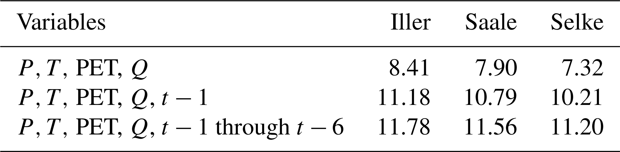
Table 6Conditional entropy of the input data regarding discharge, with and without the consideration of memory. Note that the values of the conditional entropy are not directly comparable to the values of the joint entropy in Table 5.
3.4 Experiment 4: do spatially distributed input data carry relevant information and thus enhance learning without compromising the generality of what has been learnt?
The results of our experiment wherein we changed the spatial discretization of the model input data for the HBV model (Fig. 6) show that for the Iller and Selke catchments, the model performance is generally, i.e. for all training sample sizes, much better when the model input is semi-distributed rather than lumped. For the Saale catchment, there is also a slight performance improvement when using the semi-distributed model input, but the benefit is more pronounced for smaller training sample sizes and disappears for the larger sample sizes.
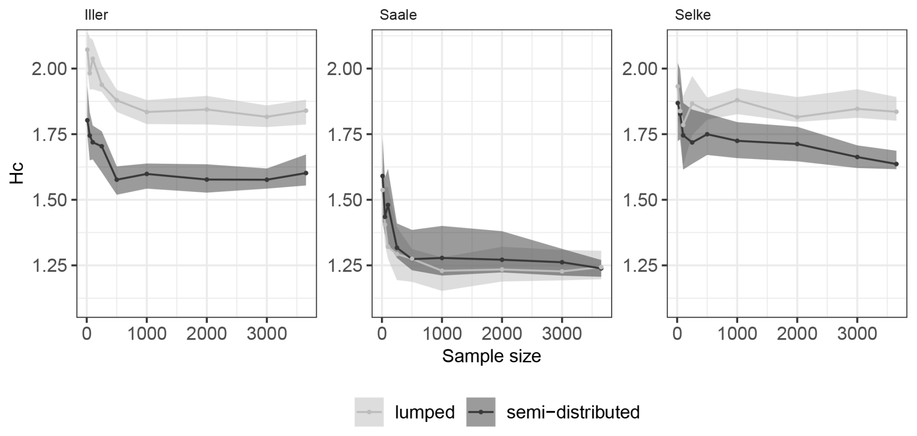
Figure 6Learning curve using different spatial discretizations of the forcing data for the HBV model, showing the changes in the conditional entropy Hc with increasing sample size. The lower the values of Hc, the more the model could learn from the data (i.e. the better the discharge simulations are). The band of the learning curves represents the 25th to 75th percentile of the ensemble of 30 repetitions, and the line is the median. The samples are independent from each other, and the lines are there only for visualization.
For the Saale catchment, there was essentially no improvement when using the semi-distributed input compared to the lumped input. Here, the sub-basins are more similar, in terms of catchment characteristics such as topography and geology but also in terms of precipitation inputs, to each other than in the Iller and Selke catchments. Therefore, the use of the lumped catchment average does not imply a great loss of information regarding the input data P,T, and PET.
For the Iller catchment, there was an offset in the performances of the HBV model when provided with both semi-distributed and lumped input data. This offset can be explained by the different sub-basins of the Iller catchment, which cover different elevation zones. This implies that also the variability of precipitation, which is related to the altitude, is significantly different from the lumped input. The same is true for temperature, which in the semi-distributed input is more likely to simulate more realistic snow accumulation and melt and seems to have a positive effect on the model performance. For the Selke catchment, there is one sub-basin that is higher than the rest of the catchment and receives more precipitation than the other two sub-basins, and resolving this more closely in the semi-distributed input may explain the gain in model performance when using the semi-distributed input rather than a lumped catchment average.
While the shapes of the learning curves for the Iller catchment are similar, the shapes of the semi-distributed versus the lumped HBV model inputs for the Selke catchment are not. Here, it appears that not only the performance improves but also there is an improved learning both for the small sample sizes and still for the larger sample sizes. The learning curves of the HBV model in the Selke catchment are again with better performance throughout and show this slight learning advantage when using the semi-distributed input. There is a sub-basin that is very different from the rest in terms of elevation, and accounting for this in the input might help the model to better capture the dynamics. The better learning compared to the lumped input suggests that specifically accounting for this sub-basin and its variability provides useful information in the additional data with increasing sample size that would be smoothed out for the lumped input.
The benefit of a more spatially explicit input to the HBV model has been previously investigated for other regions. Lopez and Seibert (2016) found improved model performance (Nash–Sutcliffe efficiency), but as we also found, the improvement was site-specific and very variable for a pre-Alpine region with a strong climatic gradient in Switzerland. Huang et al. (2019) looked at four catchments in Baden-Württemberg, Germany, and found only marginal model improvement with higher spatial discretization of the input data, but in their study, the higher spatial discretization came from resolving elevation zones rather than sub-catchments.
3.5 Limitations of the study design
There are several limitations in the study design, mainly due to choices made explicitly for the experiment but also due to model-specific constraints and feasibility.
We chose a consistent LHS for all models (see details in Supplementary Material) regardless of the number of parameters. However, if the LHS is too small for the parameter space spanned by the parameters of a (hydrological) model, this can lead to significant limitations. A small sample size may not adequately capture the variability and complexity of the input parameters, resulting in biased or incomplete representations of the model's behaviour. This can generally lead to underestimation of uncertainties and also impact the interpretation of the learning curves. Therefore, the interpretation of the model learning, especially for models with a larger number of parameters, needs to be done carefully. Another approach would be to derive learning curves from the parameter samples drawn by a gradient-based optimization algorithm (e.g. shuffled-complex evolution). This approach would have the challenge of needing to be consistently applied to all investigated methods.
The data are not exactly the same for all models, although we have tried to make them as similar as possible in this framework. Part of the difference in the learning abilities of the models could be explained by the different discretizations used to form the actual model forcing from the exact same gridded meteorological data provided as input for all models. However, the question of which model was the best learner – apart from LSTM, which clearly stood out – could not be answered directly from the discretization used for each model. Instead, we found that this was different for the three study catchments. In this study, we have relied on daily data only and have therefore not been able to include an assessment of faster processes on a sub-daily scale. Particularly when using models for specific purposes such as flood forecasting, where these faster processes are relevant, it would be important to include higher-resolution data.
We argued that the additional data used by some models, such as the soil types and land use types used in SWAT+ but not in the simpler process-based models and not in the data-driven models, are part of the model itself and could therefore be considered as the model architecture itself. It may be that these additional data are beneficial to model performance, but this was not evident from our results.
It should also be noted that there is uncertainty in the data and that measurement or interpolation errors have not been explicitly investigated in this study. Certain types of models can deal with this in the sense that they would adapt to the data provided to them. For example, data-driven models would still find a statistical relationship between meteorological input and discharge, even though parts of the data may contain substantial errors. For the process-based models, the model structure does not allow such a high degree of flexibility, and this may be reflected in poor model performance. Within the family of process-based models, the less complex models that were designed to focus on runoff prediction, such as HBV or GR4J, can still provide a rather flexible way of attempting to model the input–response relationship through the choice of model parameters, whereas the more complex process-based models with higher spatial resolution, focusing on different hydrological processes within the catchment and using runoff as a means of evaluating the model, have much less flexibility. This means that they will not perform well if the data used to force and evaluate the model are error-prone.
We have studied only three catchments in Germany. These catchments are different from each other, but more in terms of topography and local climatology than in terms of different climate zones. We chose these example catchments in order to be able to find some explanations for the different learning of the models, the different data variability, and the learnability. The influence of the elevation included in the model and also the processes that most influence the catchment response are probably represented using these three catchments, at least for the catchments in Central Europe, i.e. high-elevation catchments with snow influence, hilly mid-mountain catchments, and catchments with some lowland coverage. Some of the results are probably site-specific and not transferable to other catchments. For example, the Selke catchment has a very distinct sub-basin with a steep topography, and the semi-distributed data may not help learning compared to a lumped data input to the HBV model. The methodology could be applied to a larger set of models, focusing, from a large sample point of view, on how much variability correlates with learnability. However, using the three catchments allowed a more detailed look at each of them.
The choice of our study catchments, all in a humid environment, makes it difficult to draw more general conclusions about the transferability of our results. While model performance tends to decrease when moving from humid to semi-arid or arid regions, we can only speculate about the effects on the learnability of the different models in other regions of the world. For example, in a semi-arid or arid environment, the process-based models may lose some of their advantage in the early stages of learning, as the data pool available for calibration of the storage changes in representativeness. The extent to which the learning curves of the different model types would simply follow a consistent decline in performance from the beginning to the end of the learning curve, or whether this would actually result in different slopes of the curves, is an interesting question for future research.
Learning in our study setup is limited to constraining and evaluating discharge and does not consider other variables such as evapotranspiration or the groundwater table. The results presented may change using other and additional variables to evaluate the learning. We would not expect a huge change in the general learning behaviour when comparing data-driven and process-based models but a change in the shape of the learning curve with a general slowing down of the learning rate. How the ranking of the different process-based models would be affected cannot be answered here but would be interesting to investigate in the future.
3.6 Information theoretical measures in hydrological studies
Information theory can be a powerful tool to address hydrological problems. One advantage is the dimensionless evaluation of probabilities connected to data rather than the evaluation of their original values. This allows the variability of all data used for modelling to be estimated in the single metric “joint entropy”. The study catchments and their data could be compared with the joint entropy, showing that, in our case, the highest variability was found in the Iller catchment and the lowest in the Selke catchment. In order to investigate the relation of the variability of the data and learnability of a predictive model thereof, we compared the unconditional entropy of the dataset with the conditional entropy of discharge given all other variables. Here, the order of the catchments was reversed: the Iller catchment, despite the highest data variability, also showed the smallest conditional entropy of discharge, i.e. had the highest learnability. The Selke catchment, on the contrary, had the lowest unconditional joint entropy of the catchment variables, but also the highest conditional entropy, i.e. lowest learnability of the data.
Comparing the ranking of the different models when evaluating the performance using the information theory metric “conditional entropy” and the more commonly used hydrological metric “KGE”, only small differences were found. However, using the information theory metric allowed a more direct comparison with the conditional entropy we calculated to express the learnability of the catchments.
Comparing the learning curves of different models is also very useful in terms of how much of a learner the model itself is, despite the model's starting or ending performance and ranking in performance. What is more interesting is the learning from start to finish and when the models stop learning.
There are issues when comparing catchments with classic hydrological performance metrics, because even though standardized or normalized in their scale, these metrics do not provide an indication of how the model performs in absolute terms (Schaefli and Gupta, 2007). Some authors hence strongly advocate for benchmarks in hydrology that consider the catchment's complexity and the difficulty to simulate hydrological processes in a region (Seibert, 2001; Schaefli and Gupta, 2007; Pappenberger et al., 2015; Seibert et al., 2018; Knoben, 2024). Using information measures throughout the entire workflow of data analysis, model training, and model evaluation in hydrology could help mitigate this issue but is currently rarely done. Whereas in very few studies (Jiang et al., 2022, 2024b), information measures are used for specific parts, for final model evaluation, usually well-known metrics such as KGE and Nash–Sutcliffe efficiency are used for easier interpretation by the readers.
In this study, we investigated how different models can make use of the information in discharge data and what kind of data is most useful for models. To do this, we carried out four experiments: the main experiment, experiment 1, was designed to assess the differences in the learning capabilities of different models, four of them data-driven and four process-based, with varying degrees of complexity. Experiments 2 and 4 were designed to answer related questions about learning with different sampling schemes and spatial discretization of the input data. We also investigated how much this varies for different catchment types in a humid climate, including the transition zone from the Harz to the central German lowlands, the mid-range mountains, and the Alpine region of Germany. In experiment 3, we investigated whether it is possible to predict how well models can deal with a given dataset. For this experiment, we used information theory to describe both the variability in all the data used by the model and the learnability, in the sense of how much information in the data could actually be useful for a model predicting discharge, using joint and conditional entropy.
There is a difference between how variable the dataset of a particular catchment is (in this study, measured by joint entropy) and how easy it is to learn from it (in this study, measured by the conditional entropy of discharge given the input data). The perhaps intuitive notion that the more variable the data for a given catchment, the more difficult it is to learn from it, does not hold. We also found that different models are different learners and that this varies also for the catchment for which they are set up. That means the different learners are not performing equally well for all catchments, and the ranking of which was the best learner varies.
In general, however, the process-based models used in our study initially know more than the data-driven models due to their model architecture, which includes some memory capabilities and thus the ability to account for memory. While this fixed model architecture appears to be advantageous at the beginning of the learning, i.e when only few data points are provided for training, process-based models stop learning relatively soon and plateau at a certain model performance, i.e. after a certain amount of data has been included. On the contrary, the data-driven LSTM model had very poor performance at the beginning of the learning curve and then learnt quickly and steadily as more data were provided for training. The LSTM continued to learn after all the process-based models stopped learning and is very useful as a benchmark learner.
The LSTM model's ability to learn through its flexible approach, combined with the fixed structural architecture that gives process-based models an advantage in data-poor settings, raises the compelling – though as yet unresolved – question of whether hybrid architectures could effectively integrate these complementary strengths.
Applying three different sampling schemes to provide the same sample size for training showed that a fully random sampling provides the best basis for learning, consecutive random sampling – as it would be realistic from different sampling campaigns over a period – reached a similar performance for a large sample size, and, surprisingly, the optimal sampling using the Douglas–Peucker algorithm did not outperform the two random sampling schemes in the tested catchments. A possible explanation for the poorer-than-expected results of the Douglas–Peucker method could be that the hydrological catchment response is a function of the interplay of short-, intermediate- and long-term storage, which requires adequate parameterization of the related storage functions in the model. Random sampling selects a time-proportional share of low flow, intermediate flow, and high flow situations, which gives the model the opportunity to learn the correct parameterization of baseflow, interflow, and fast runoff processes. Douglas–Peucker sampling selects the main “turning points” in a time series, which occur at the onset and peak of high-flow events, and may thus leave the model little opportunity to learn about long-term processes. We hypothesize that a hybrid combination of randomly selected points with Douglas–Peucker selected points may yield the best results. We leave this for future investigations.
Regarding the spatial discretization of the input data from sub-catchment to lumped, we found that reducing the spatial discretization of the meteorological input to the model resulted in an overall decrease in performance, the extent of which, not surprisingly, depends on the homogeneity of the catchment and, in our cases, to a large extent on the forcing data in the different sub-catchments. We have considered only the effect of meteorological forcing at different resolutions, but other data may be relevant for this catchment, which showed the least improvement.
Joint entropy is a simple yet powerful way of estimating the variability of the data associated with a catchment, as it can handle data that come with different dimensions. Conditional entropy tells us how these data can be used to predict discharge. When no memory is taken into account, the conditional entropy is large, but as soon as some memory is introduced in the form of aggregations of variables over the current and past day or past week, the conditional entropy becomes smaller, indicating that memory is a very important component of the data and that capturing it improves the model performance. This was particularly evident in the catchment from the low mountain ranges and the Alpine region.
Table A1Properties of information-based compared to value-based distance measures between model simulations and corresponding observations.
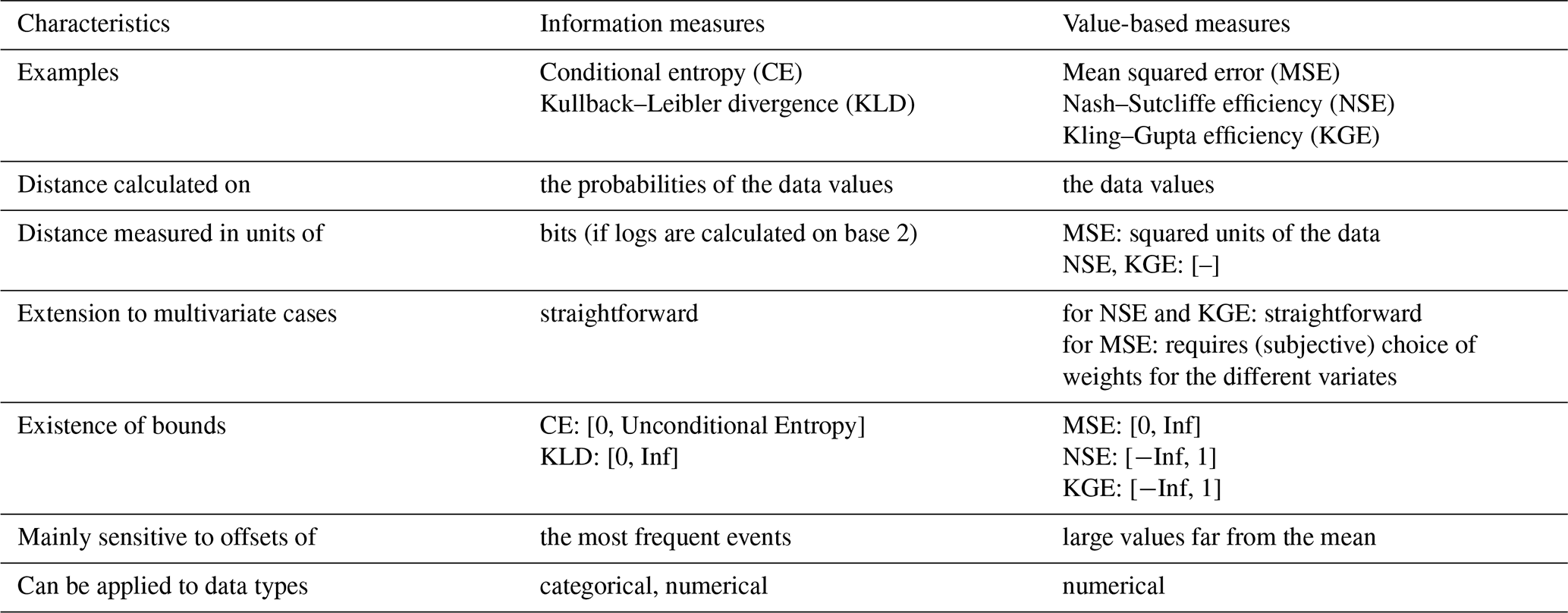
The code to calculate the conditional entropy from the model simulations, input data, and discharge data is provided through a GitHub repository at https://github.com/MariStau/IMPRO_infotheory_Data_Code (last access: 27 July 2025) and via Zenodo at https://doi.org/10.5281/zenodo.14938050 (Staudinger and Ehret, 2025).
This publication has been prepared using the European Union's Copernicus Land Monitoring Service information: https://doi.org/10.2909/960998c1-1870-4e82-8051-6485205ebbac (CLMS, 2019). The digital elevation models of the catchments were retrieved from http://hydro.iis.u-tokyo.ac.jp/~yamadai/MERIT_Hydro/ (last access: 27 July 2025) (Yamazaki et al., 2019). The model input data and results are provided through a GitHub repository at https://github.com/MariStau/IMPRO_infotheory_Data_Code (last access: 27 July 2025) and via Zenodo at https://doi.org/10.5281/zenodo.14938050 (Staudinger and Ehret, 2025).
The supplement related to this article is available online at https://doi.org/10.5194/hess-29-5005-2025-supplement.
Conceptualization and methodology: UE and MS. Data curation: AH and ST. Investigation and formal analysis: MS, UE, AH, TH, RL, JM, and DS. Funding acquisition: BG. Visualization: MS and AH. Writing – initial draft: MS, UE, and SP. Writing – review and editing: all authors. All authors have read and agreed to the published version of the paper.
At least one of the (co-)authors is a member of the editorial board of Hydrology and Earth System Sciences. The peer-review process was guided by an independent editor, and the authors also have no other competing interests to declare.
Publisher’s note: Copernicus Publications remains neutral with regard to jurisdictional claims made in the text, published maps, institutional affiliations, or any other geographical representation in this paper. While Copernicus Publications makes every effort to include appropriate place names, the final responsibility lies with the authors.
For providing the discharge data, we thank these three local authorities in Germany: LfU Bavaria, TLUBN Thuringia, and LHW Saxonia-Anhalt. Simulations were performed with computing resources provided by ZIM, University of Potsdam. We thank Salvatore Manfreda and Claudia Brauer for their valuable comments and suggestions during the review process, which helped us to improve the paper considerably.
This research has been supported by the Deutsche Forschungsgemeinschaft (grant no. 471280762).
This paper was edited by Nunzio Romano and reviewed by Salvatore Manfreda and Claudia Brauer.
Abhinav, G. and Rao, S. G.: Uncertainty quantification in watershed hydrology: Which method to use?, Journal of Hydrology, 616, 128749, https://doi.org/10.1016/j.jhydrol.2022.128749, 2023. a
Acuña Espinoza, E., Loritz, R., Álvarez Chaves, M., Bäuerle, N., and Ehret, U.: To bucket or not to bucket? Analyzing the performance and interpretability of hybrid hydrological models with dynamic parameterization, Hydrol. Earth Syst. Sci., 28, 2705–2719, https://doi.org/10.5194/hess-28-2705-2024, 2024. a, b, c
Arnold, J. G., Srinivasan, R., Muttiah, R. S., and Williams, J. R.: Large area hydrologic modeling and assessment part I: model development 1, JAWRA Journal of the American Water Resources Association, 34, 73–89, 1998. a
Ayzel, G. and Heistermann, M.: The effect of calibration data length on the performance of a conceptual hydrological model versus LSTM and GRU: A case study for six basins from the CAMELS dataset, Computers & Geosciences, 149, 104708, https://doi.org/10.1016/j.cageo.2021.104708, 2021. a
Azmi, E., Ehret, U., Weijs, S. V., Ruddell, B. L., and Perdigão, R. A. P.: Technical note: “Bit by bit”: a practical and general approach for evaluating model computational complexity vs. model performance, Hydrol. Earth Syst. Sci., 25, 1103–1115, https://doi.org/10.5194/hess-25-1103-2021, 2021. a
BGR: Bodenuebersichtskarte im Massstab 1:200000, Verbreitung der Bodengesellschaften, https://www.bgr.bund.de/DE/Themen/Boden/Projekte/Flaechen_Rauminformationen_Boden/BUEK200/BUEK200.html (last access: 29 September 2025), 1999. a
Bieger, K., Arnold, J. G., Rathjens, H., White, M. J., Bosch, D. D., Allen, P. M., Volk, M., and Srinivasan, R.: Introduction to SWAT+, A Completely Restructured Version of the Soil and Water Assessment Tool, JAWRA Journal of the American Water Resources Association, 53, 115–130, https://doi.org/10.1111/1752-1688.12482, 2017. a
Boeing, F., Rakovec, O., Kumar, R., Samaniego, L., Schrön, M., Hildebrandt, A., Rebmann, C., Thober, S., Müller, S., Zacharias, S., Bogena, H., Schneider, K., Kiese, R., Attinger, S., and Marx, A.: High-resolution drought simulations and comparison to soil moisture observations in Germany, Hydrol. Earth Syst. Sci., 26, 5137–5161, https://doi.org/10.5194/hess-26-5137-2022, 2022. a
Brath, A., Montanari, A., and Toth, E.: Analysis of the effects of different scenarios of historical data availability on the calibration of a spatially-distributed hydrological model, Journal of Hydrology, 291, 232–253, https://doi.org/10.1016/j.jhydrol.2003.12.044, 2004. a, b
CLMS: CORINE land use, EEA geospatial data catalogue [data set], https://doi.org/10.2909/960998c1-1870-4e82-8051-6485205ebbac, 2019. a, b, c
Correa, A., Windhorst, D., Crespo, P., Célleri, R., Feyen, J., and Breuer, L.: Continuous versus event-based sampling: how many samples are required for deriving general hydrological understanding on Ecuador's páramo region?, Hydrological Processes, 30, 4059–4073, https://doi.org/10.1002/hyp.10975, 2016. a
Cover, T. and Thomas, J. A.: Elements of Information Theory, Wiley Series in Telecommunications and Signal Processing, Wiley-Interscience, ISBN 9780471241959, 2006. a
Craig, J. R., Brown, G., Chlumsky, R., Jenkinson, R. W., Jost, G., Lee, K., Mai, J., Serrer, M., Sgro, N., Shafii, M., Snowdon, A. P., and Tolson, B. A.: Flexible watershed simulation with the Raven hydrological modelling framework, Environmental Modelling & Software, 129, 104728, https://doi.org/10.1016/j.envsoft.2020.104728, 2020. a
Daliakopoulos, I. N., Coulibaly, P., and Tsanis, I. K.: Groundwater level forecasting using artificial neural networks, Journal of Hydrology, 309, 229–240, 2005. a
De la Fuente, L. A., Ehsani, M. R., Gupta, H. V., and Condon, L. E.: Toward interpretable LSTM-based modeling of hydrological systems, Hydrol. Earth Syst. Sci., 28, 945–971, https://doi.org/10.5194/hess-28-945-2024, 2024. a
Devia, G. K., Ganasri, B., and Dwarakish, G.: A Review on Hydrological Models, Aquatic Procedia, 4, 1001–1007, https://doi.org/10.1016/j.aqpro.2015.02.126, 2015. a
Douglas, D. H. and Peucker, T. K.: Algorithms for the reduction of the number of points required to represent a digitized line or its caricature, Cartographica: The International Journal for Geographic Information and Geovisualization, 10, 112–122, 1973. a
Ehret, U. and Dey, P.: Technical note: Complexity–uncertainty curve (c-u-curve) – a method to analyse, classify and compare dynamical systems, Hydrol. Earth Syst. Sci., 27, 2591–2605, https://doi.org/10.5194/hess-27-2591-2023, 2023. a
Fan, H., Jiang, M., Xu, L., Zhu, H., Cheng, J., and Jiang, J.: Comparison of long short term memory networks and the hydrological model in runoff simulation, Water, 12, 175, https://doi.org/10.3390/w12010175, 2020. a
Foroozand, H. and Weijs, S. V.: Objective functions for information-theoretical monitoring network design: what is “optimal”?, Hydrol. Earth Syst. Sci., 25, 831–850, https://doi.org/10.5194/hess-25-831-2021, 2021. a
Girihagama, L., Naveed Khaliq, M., Lamontagne, P., Perdikaris, J., Roy, R., Sushama, L., and Elshorbagy, A.: Streamflow modelling and forecasting for Canadian watersheds using LSTM networks with attention mechanism, Neural Computing and Applications, 34, 19995–20015, 2022. a
Gupta, H. V., Kling, H., Yilmaz, K. K., and Martinez, G. F.: Decomposition of the mean squared error and NSE performance criteria: Implications for improving hydrological modelling, Journal of Hydrology, 377, 80–91, https://doi.org/10.1016/j.jhydrol.2009.08.003, 2009. a
Guse, B., Pfannerstill, M., Kiesel, J., Strauch, M., Volk, M., and Fohrer, N.: Analysing spatio-temporal process and parameter dynamics in models to characterise contrasting catchments, J. Hydrol., 507, 863–874, https://doi.org/10.1016/j.jhydrol.2018.12.050, 2019. a
Hargreaves, G. H. and Samani, Z. A.: Reference crop evapotranspiration from temperature, Applied Engineering in Agriculture, 1, 96–99, 1985. a, b
Harlin, J.: Development of a process oriented calibration scheme for the HBV hydrological model, Hydrology Research, 22, 15–36, 1991. a
Houska, T., Kraft, P., Chamorro-Chavez, A., and Breuer, L.: SPOTting Model Parameters Using a Ready-Made Python Package, PLOS ONE, 10, 1–22, https://doi.org/10.1371/journal.pone.0145180, 2015. a
Hsu, K.-l., Gupta, H. V., and Sorooshian, S.: Artificial Neural Network Modeling of the Rainfall-Runoff Process, Water Resources Research, 31, 2517–2530, https://doi.org/10.1029/95WR01955, 1995. a
Huang, Y., Bárdossy, A., and Zhang, K.: Sensitivity of hydrological models to temporal and spatial resolutions of rainfall data, Hydrol. Earth Syst. Sci., 23, 2647–2663, https://doi.org/10.5194/hess-23-2647-2019, 2019. a
Jiang, P., Pin, S., Alexander, Y. S., and Xingyuan, C.: Optimizing parameter learning and calibration in an integrated hydrological model: Impact of observation length and information, Journal of Hydrology, 643, 131889, https://doi.org/10.1016/j.jhydrol.2024.131889, 2024a. a
Jiang, P., Shuai, P., Sun, A. Y., and Chen, X.: Optimizing parameter learning and calibration in an integrated hydrological model: Impact of observation length and information, Journal of Hydrology, 643, 131889, https://doi.org/10.1016/j.jhydrol.2024.131889, 2024b. a
Jiang, S., Zheng, Y., Wang, C., and Babovic, V.: Uncovering Flooding Mechanisms Across the Contiguous United States Through Interpretive Deep Learning on Representative Catchments, Water Resources Research, 58, e2021WR030185, https://doi.org/10.1029/2021WR030185, 2022. a
Knoben, W. J. M.: Setting expectations for hydrologic model performance with an ensemble of simple benchmarks, Hydrological Processes, 38, e15288, https://doi.org/10.1002/hyp.15288, 2024. a
Kratzert, F., Klotz, D., Brenner, C., Schulz, K., and Herrnegger, M.: Rainfall–runoff modelling using Long Short-Term Memory (LSTM) networks, Hydrol. Earth Syst. Sci., 22, 6005–6022, https://doi.org/10.5194/hess-22-6005-2018, 2018. a, b, c
Kratzert, F., Gauch, M., Klotz, D., and Nearing, G.: HESS Opinions: Never train a Long Short-Term Memory (LSTM) network on a single basin, Hydrol. Earth Syst. Sci., 28, 4187–4201, https://doi.org/10.5194/hess-28-4187-2024, 2024. a
Kuana, L. A., Almeida, A. S., Mercuri, E. G. F., and Noe, S. M.: Regionalization of GR4J model parameters for river flow prediction in Paraná, Brazil, Hydrol. Earth Syst. Sci., 28, 3367–3390, https://doi.org/10.5194/hess-28-3367-2024, 2024. a
Kumar, P. and Gupta, H. V.: Debates – Does Information Theory Provide a New Paradigm for Earth Science?, Water Resources Research, 56, e2019WR026398, https://doi.org/10.1029/2019WR026398, 2020. a
Lopez, M. G. and Seibert, J.: Influence of hydro-meteorological data spatial aggregation on streamflow modelling, Journal of Hydrology, 541, 1212–1220, 2016. a
Loritz, R., Dolich, A., Acuña Espinoza, E., Ebeling, P., Guse, B., Götte, J., Hassler, S. K., Hauffe, C., Heidbüchel, I., Kiesel, J., Mälicke, M., Müller-Thomy, H., Stölzle, M., and Tarasova, L.: CAMELS-DE: hydro-meteorological time series and attributes for 1582 catchments in Germany, Earth Syst. Sci. Data, 16, 5625–5642, https://doi.org/10.5194/essd-16-5625-2024, 2024. a
Mai, J.: Ten strategies towards successful calibration of environmental models, Journal of Hydrology, 620, 129414, https://doi.org/10.1016/j.jhydrol.2023.129414, 2023. a
Mai, J., Shen, H., Tolson, B. A., Gaborit, É., Arsenault, R., Craig, J. R., Fortin, V., Fry, L. M., Gauch, M., Klotz, D., Kratzert, F., O'Brien, N., Princz, D. G., Rasiya Koya, S., Roy, T., Seglenieks, F., Shrestha, N. K., Temgoua, A. G. T., Vionnet, V., and Waddell, J. W.: The Great Lakes Runoff Intercomparison Project Phase 4: the Great Lakes (GRIP-GL), Hydrol. Earth Syst. Sci., 26, 3537–3572, https://doi.org/10.5194/hess-26-3537-2022, 2022. a
Melsen, L., Teuling, A., Van Berkum, S., Torfs, P., and Uijlenhoet, R.: Catchments as simple dynamical systems: A case study on methods and data requirements for parameter identification, Water Resources Research, 50, 5577–5596, 2014. a, b
Moges, E., Ruddell, B. L., Zhang, L., Driscoll, J. M., and Larsen, L. G.: Strength and Memory of Precipitation's Control Over Streamflow Across the Conterminous United States, Water Resources Research, 58, e2021WR030186, https://doi.org/10.1029/2021WR030186, 2022. a
Mohanty, S., Jha, M. K., Raul, S., Panda, R., and Sudheer, K.: Using artificial neural network approach for simultaneous forecasting of weekly groundwater levels at multiple sites, Water Resources Management, 29, 5521–5532, 2015. a
Nearing, G. S., Ruddell, B. L., Clark, M. P., Nijssen, B., and Peters-Lidard, C.: Benchmarking and Process Diagnostics of Land Models, Journal of Hydrometeorology, 19, 1835–1852, https://doi.org/10.1175/JHM-D-17-0209.1, 2018. a
Neuper, M. and Ehret, U.: Quantitative precipitation estimation with weather radar using a data- and information-based approach, Hydrol. Earth Syst. Sci., 23, 3711–3733, https://doi.org/10.5194/hess-23-3711-2019, 2019. a, b
Paez-Trujilo, A., Cañon, J., Hernandez, B., Corzo, G., and Solomatine, D.: Multivariate regression trees as an “explainable machine learning” approach to explore relationships between hydroclimatic characteristics and agricultural and hydrological drought severity: case of study Cesar River basin, Nat. Hazards Earth Syst. Sci., 23, 3863–3883, https://doi.org/10.5194/nhess-23-3863-2023, 2023. a
Pappenberger, F., Ramos, M., Cloke, H., Wetterhall, F., Alfieri, L., Bogner, K., Mueller, A., and Salamon, P.: How do I know if my forecasts are better? Using benchmarks in hydrological ensemble prediction, Journal of Hydrology, 522, 697–713, https://doi.org/10.1016/j.jhydrol.2015.01.024, 2015. a
Perrin, C., Michel, C., and Andréassian, V.: Improvement of a parsimonious model for streamflow simulation, Journal of Hydrology, 279, 275–289, https://doi.org/10.1016/S0022-1694(03)00225-7, 2003. a
Perrin, C., Oudin, L., Andreassian, V., Rojas-Serna, C., Michel, C., and Mathevet, T.: Impact of limited streamflow data on the efficiency and the parameters of rainfall – runoff models, Hydrological Sciences Journal, 52, 131–151, 2007. a
Pool, S. and Seibert, J.: Gauging ungauged catchments – Active learning for the timing of point discharge observations in combination with continuous water level measurements, Journal of Hydrology, 598, 126448, https://doi.org/10.1016/j.jhydrol.2021.126448, 2021. a
Pool, S., Viviroli, D., and Seibert, J.: Prediction of hydrographs and flow-duration curves in almost ungauged catchments: Which runoff measurements are most informative for model calibration?, Journal of Hydrology, 554, 613–622, 2017. a
Rakovec, O., Kumar, R., Mai, J., Cuntz, M., Thober, S., Zink, M., Attinger, S., Schäfer, D., Schrön, M., and Samaniego, L.: Multiscale and Multivariate Evaluation of Water Fluxes and States over European River Basins, Journal of Hydrometeorology, 17, 287–307, https://doi.org/10.1175/JHM-D-15-0054.1, 2016. a
Ramer, U.: An iterative procedure for the polygonal approximation of plane curves, Computer Graphics and Image Processing, 1, 244–256, https://doi.org/10.1016/S0146-664X(72)80017-0, 1972. a
Reichstein, M., Camps-Valls, G., Stevens, B., Jung, M., Denzler, J., Carvalhais, N., and Prabhat: Deep learning and process understanding for data-driven Earth system science, Nature, 566, 195–204, https://doi.org/10.1038/s41586-019-0912-1, 2019. a
Renteria-Mena, J. B., Plaza, D., and Giraldo, E.: Multivariable NARX Based Neural Networks Models for Short-Term Water Level Forecasting, Engineering Proceedings, 39, 60, https://doi.org/10.3390/engproc2023039060, 2023. a
Rojas-Serna, C., Michel, C., Perrin, C., Andréassian, V., Hall, A., Chahinian, N., and Schaake, J.: Ungauged catchments: how to make the most of a few streamflow measurements?, IAHS Publication, 307, 230, https://iahs.info/uploads/dms/13616.23-230-236-43-ROJAS-SERNA.pdf (last access: 29 September 2025), 2006. a
Ruddell, B. L., Drewry, D. T., and Nearing, G. S.: Information Theory for Model Diagnostics: Structural Error is Indicated by Trade-Off Between Functional and Predictive Performance, Water Resources Research, 55, 6534–6554, https://doi.org/10.1029/2018WR023692, 2019. a
Schaefli, B. and Gupta, H. V.: Do Nash values have value?, Hydrological Processes, 21, 2075–2080, 2007. a, b
Schoppa, L., Disse, M., and Bachmair, S.: Evaluating the performance of random forest for large-scale flood discharge simulation, Journal of Hydrology, 590, 125531, https://doi.org/10.1016/j.jhydrol.2020.125531, 2020. a
Seibert, J.: On the need for benchmarks in hydrological modelling, Hydrological Processes, 15, 1063–1064, https://doi.org/10.1002/hyp.446, 2001. a, b
Seibert, J. and Beven, K. J.: Gauging the ungauged basin: how many discharge measurements are needed?, Hydrol. Earth Syst. Sci., 13, 883–892, https://doi.org/10.5194/hess-13-883-2009, 2009. a
Seibert, J. and Vis, M. J. P.: Teaching hydrological modeling with a user-friendly catchment-runoff-model software package, Hydrol. Earth Syst. Sci., 16, 3315–3325, https://doi.org/10.5194/hess-16-3315-2012, 2012. a
Seibert, J., Vis, M. J. P., Lewis, E., and van Meerveld, H.: Upper and lower benchmarks in hydrological modelling, Hydrological Processes, 32, 1120–1125, https://doi.org/10.1002/hyp.11476, 2018. a
Shen, C.: A transdisciplinary review of deep learning research and its relevance for water resources scientists, Water Resources Research, 54, 8558–8593, 2018. a
Shen, C., Appling, A. P., Gentine, P., Bandai, T., Gupta, H., Tartakovsky, A., Baity-Jesi, M., Fenicia, F., Kifer, D., Li, L., Liu, X., Ren, W., Zheng, Y., Harman, C. J., Clark, M., Farthing, M., Feng, D., Kumar, P., Aboelyazeed, D., Rahmani, F., Song, Y., Beck, H. E., Bindas, T., Dwivedi, D., Fang, K., Höge, M., Rackauckas, C., Mohanty, B., Roy, T., Xu, C., and Lawson, K.: Differentiable modelling to unify machine learning and physical models for geosciences, Nature Reviews Earth & Environment, 4, 552–567, https://doi.org/10.1038/s43017-023-00450-9, 2023. a
Shen, H., Tolson, B. A., and Mai, J.: Time to Update the Split-Sample Approach in Hydrological Model Calibration, Water Resources Research, 58, e2021WR031523, https://doi.org/10.1029/2021WR031523, 2022. a
Singh, S. K. and Bárdossy, A.: Calibration of hydrological models on hydrologically unusual events, Advances in Water Resources, 38, 81–91, https://doi.org/10.1016/j.advwatres.2011.12.006, 2012. a, b
Sippel, S., Lange, H., Mahecha, M. D., Hauhs, M., Bodesheim, P., Kaminski, T., Gans, F., and Rosso, O. A.: Diagnosing the Dynamics of Observed and Simulated Ecosystem Gross Primary Productivity with Time Causal Information Theory Quantifiers, PLOS ONE, 11, e0164960, https://doi.org/10.1371/journal.pone.0164960, 2016. a
Smith, K. A., Barker, L. J., Tanguy, M., Parry, S., Harrigan, S., Legg, T. P., Prudhomme, C., and Hannaford, J.: A multi-objective ensemble approach to hydrological modelling in the UK: an application to historic drought reconstruction, Hydrol. Earth Syst. Sci., 23, 3247–3268, https://doi.org/10.5194/hess-23-3247-2019, 2019. a
Snieder, E. and Khan, U. T.: A diversity-centric strategy for the selection of spatio-temporal training data for LSTM-based streamflow forecasting, Hydrol. Earth Syst. Sci., 29, 785–798, https://doi.org/10.5194/hess-29-785-2025, 2025. a
Sun, W., Wang, Y., Wang, G., Cui, X., Yu, J., Zuo, D., and Xu, Z.: Physically based distributed hydrological model calibration based on a short period of streamflow data: case studies in four Chinese basins, Hydrol. Earth Syst. Sci., 21, 251–265, https://doi.org/10.5194/hess-21-251-2017, 2017. a, b, c
Staudinger, M. and Ehret, U.: MariStau/IMPRO_infotheory_Data_Code: Data and code used to calculate conditional entropy values, Zenodo [code and data set], https://doi.org/10.5281/zenodo.14938050, 2025. a, b
Tolson, B. A., Asadzadeh, M., Maier, H. R., and Zecchin, A.: Hybrid discrete dynamically dimensioned search (HD-DDS) algorithm for water distribution system design optimization, Water Resources Research, 45, 12, https://doi.org/10.1029/2008WR007673, 2009. a
Valéry, A., Andréassian, V., and Perrin, C.: “As simple as possible but not simpler”: What is useful in a temperature-based snow-accounting routine? Part 2 – Sensitivity analysis of the Cemaneige snow accounting routine on 380 catchments, Journal of Hydrology, 517, 1176–1187, https://doi.org/10.1016/j.jhydrol.2014.04.058, 2014. a
Vrugt, J. A., Gupta, H. V., Dekker, S. C., Sorooshian, S., Wagener, T., and Bouten, W.: Application of stochastic parameter optimization to the Sacramento Soil Moisture Accounting model, Journal of Hydrology, 325, 288–307, 2006. a, b
Wagner, P. D., Duethmann, D., Kiesel, J., Pool, S., Hrachowitz, M., Ceola, S., Herzog, A., Houska, T., Loritz, R., Spieler, D., Staudinger, M., Tarasova, L., Thober, S., Fohrer, N., Tetzlaff, D., Wagener, T., and Guse, B.: The Unexploited Treasures of Hydrological Observations Beyond Streamflow for Catchment Modeling, WIREs Water, 12, e70018, https://doi.org/10.1002/wat2.70018, 2025. a
Wright, D. P., Thyer, M., Westra, S., and McInerney, D.: A hybrid framework for quantifying the influence of data in hydrological model calibration, Journal of Hydrology, 561, 211–222, 2018. a
Xiang, Z., Yan, J., and Demir, I.: A Rainfall-Runoff Model With LSTM-Based Sequence-to-Sequence Learning, Water Resources Research, 56, e2019WR025326, https://doi.org/10.1029/2019WR025326, 2020. a
Yamazaki, D., Ikeshima, D., Sosa, J., Bates, P. D., Allen, G. H., and Pavelsky, T. M.: MERIT Hydro: A High-Resolution Global Hydrography Map Based on Latest Topography Dataset, Water Resources Research, 55, 5053–5073, https://doi.org/10.1029/2019WR024873, 2019 (data available at: http://hydro.iis.u-tokyo.ac.jp/~yamadai/MERIT_Hydro/, last access: 29 September 2025). a, b
Yapo, P. O., Gupta, H. V., and Sorooshian, S.: Automatic calibration of conceptual rainfall-runoff models: sensitivity to calibration data, Journal of Hydrology, 181, 23–48, https://doi.org/10.1016/0022-1694(95)02918-4, 1996. a, b
Zhang, K., Luhar, M., Brunner, M. I., and Parolari, A. J.: Streamflow Prediction in Poorly Gauged Watersheds in the United States Through Data-Driven Sparse Sensing, Water Resources Research, 59, e2022WR034092, https://doi.org/10.1029/2022WR034092, 2023. a, b
Zhang, Y., Chiew, F. H. S., Li, M., and Post, D.: Predicting Runoff Signatures Using Regression and Hydrological Modeling Approaches, Water Resources Research, 54, 7859–7878, https://doi.org/10.1029/2018WR023325, 2018. a
Zhang, Y., Ragettli, S., Molnar, P., Fink, O., and Peleg, N.: Generalization of an Encoder-Decoder LSTM model for flood prediction in ungauged catchments, Journal of Hydrology, 614, 128577, https://doi.org/10.1016/j.jhydrol.2022.128577, 2022. a
Zink, M., Kumar, R., Cuntz, M., and Samaniego, L.: A high-resolution dataset of water fluxes and states for Germany accounting for parametric uncertainty, Hydrol. Earth Syst. Sci., 21, 1769–1790, https://doi.org/10.5194/hess-21-1769-2017, 2017. a, b