the Creative Commons Attribution 4.0 License.
the Creative Commons Attribution 4.0 License.
Downscaling the probability of heavy rainfall over the Nordic countries
Rasmus E. Benestad
Kajsa M. Parding
Andreas Dobler
We used empirical–statistical downscaling to derive local statistics for 24 h and sub-daily precipitation over the Nordic countries, based on large-scale information provided by global climate models. The local statistics included probabilities for heavy precipitation and intensity–duration–frequency (IDF) curves for sub-daily rainfall. The downscaling was based on estimating key parameters defining the shape of mathematical curves describing probabilities and return values, namely the annual wet-day frequency, fw, and the wet-day mean precipitation, μ. Both parameters were used as predictands representing local precipitation statistics as well as predictors representing large-scale conditions. We used multi-model ensembles of global climate model (CMIP6) simulations, calibrated on the ERA5 reanalysis, to derive local projections and future outlooks. Our analysis included an evaluation of how well the global climate models reproduced the predictors in addition to assessing the quality of downscaled precipitation statistics. The evaluation suggested that present global climate models capture essential aspects of the covariance, and there was a good match between annual wet-day frequency and wet-day mean precipitation derived from ERA5 on the one hand and local rain gauges in the Nordic region on the other. Furthermore, the ensemble downscaled results for annual fw and μ were approximately normally distributed, which may justify using the ensemble mean and standard deviation to describe the ensemble spread. Hence, our efforts provide a demonstration for how empirical–statistical downscaling can be used to provide practical information on heavy rainfall, which subsequently may be used for impact studies. Future projections for the Nordic region indicated little increase in precipitation due to more wet days, but most of the contribution comes from increased mean intensity. The west coast of Norway had the highest probabilities of receiving more than 30 mm d−1 precipitation, but the strongest relative trend in this probability was projected over northern Finland. Furthermore, the highest estimates for trends in 10-year and 25-year return values were projected over western Norway, where they were high from the outset. Our results also suggested that future precipitation intensity is sensitive to future emissions, whereas the wet-day frequency is less sensitive.
- Article
(6998 KB) - Full-text XML
-
Supplement
(45701 KB) - BibTeX
- EndNote
Increasing atmospheric concentrations of greenhouse gases, such as carbon dioxide (CO2) and methane (CH4) from human activity, strengthen the greenhouse effect and bring on global warming as well as changes in the global hydrological cycle (IPCC, 2021). Global climate models (GCMs) and Earth system models (ESMs1) are our primary tools for making projections of the future climate and represent main features of the Earth's climate system, but they are not designed to describe the small-scale and local climate change (Takayabu et al., 2015). Nevertheless, the local response to global warming can be estimated through downscaling (see Appendix A), and international efforts on downscaling have been coordinated under the World Climate Research Programme (WCRP) and its downscaling experiment (CORDEX) (Gutowski Jr. et al., 2016). The term downscaling in this case refers to the process of using large-scale information that GCMs are able to reproduce skilfully, on scales larger than their minimum skilful scale (Takayabu et al., 2015), and subsequently add additional information about inter-scale dependencies and systematic effects from fixed geographical factors. Hence, our definition of downscaling is different to both merely transforming the data to a finer grid mesh and bias adjustment that corrects model output so that they have similar statistical characteristics as observations without further considerations of GCMs' minimum skilful scale2. Results of GCMs are often downscaled to provide projections for a future climate on a regional or local scale, but the omnipresence of pronounced non-deterministic regional-scale decadal variability (Deser et al., 2012, 2020) represents a challenge and a source of uncertainty (Hawkins and Sutton, 2009). The non-deterministic chaotic contribution from natural and internal regional variations complicates the assessment of the credibility and robustness of ensemble projections, and one question is how to synthesize them into user-relevant information. This is highly relevant for results from downscaling approaches at national climate service levels, for instance, within the European downscaling efforts in EURO-CORDEX.
Another source of uncertainty in downscaled climate projections is connected to methodological choices and assumptions (Jacob et al., 2020). There are two main approaches in downscaling: (i) dynamical downscaling with regional climate models (RCMs) and (ii) empirical–statistical downscaling (ESD). The former has often been more visible within CORDEX, many climate service providers, and impacts and adaptation communities (Rampal et al., 2024), and CORDEX data often refer to a set of RCM simulations excluding ESD results, e.g. the IPCC Interactive Atlas (https://interactive-atlas.ipcc.ch/regional-information/about, last access: 22 December 2024). The one-sided focus may be a legacy of the past European projects PRUDENCE (2001–2004) and STARDEX (2002–2005), which had their distinct focus (Christensen et al., 2007; Christensen and Christensen, 2007; Goodess et al., 2003); however, results from STARDEX did not indicate that RCMs were superior in terms of reproducing information about extreme rainfall (Haylock et al., 2006). Traditionally, ESD has been used to estimate small-scale (local) temperature or precipitation in terms of daily variability or aggregated statistics over months, seasons, or years (Maraun et al., 2015), and downscaling of heavy precipitation has mainly involved dynamical downscaling with RCMs, while the merits of ESD have perhaps not been so widely recognized.
One advantage with ESD is that it requires little computational resources, which makes it suitable for downscaling large multi-model ensembles (Benestad, 2011; Mezghani et al., 2017). Furthermore, ESD can be designed so that it is transparent and easily traceable, as the R Markdown script in this paper's Supplement tries to facilitate (Benestad, 2024). It is also possible to estimate various statistical aspects of precipitation through ESD, and Trenberth et al. (2003) argued that the characteristics of precipitation are just as vital as the amount. The characteristics of rain may indeed be more prone to change as climate changes, and some key statistics on precipitation involve both the typical amount falling on a rainy day (wet-day mean precipitation, μ), how often it rains (wet-day frequency, fw), how much time there is between each rainfall (dry-spell duration or number of consecutive dry days, ndd), duration of wet spells (number of consecutive wet days, nwd, to account for clustering of precipitation events in time), spatial extent of the precipitation (Lussana et al., 2024), and phase (rain/snow). Here we show how ESD can be designed to extract information on precipitation statistics such as probabilities of exceeding a certain threshold and intensity–duration–frequency (IDF) curves.
There have been many studies on mean trends or extreme precipitation but fewer on moderate heavy rainfall. Extremes often involves either the general extreme value theory (GEV), calibrated with block maxima, or the general Pareto distribution with peak over threshold, thus fitting the tails of the distribution (Coles, 2001). GEV also involves fitting three parameters – location, scale, and shape – which are often not well constrained for limited samples of block maxima. Statistical models for moderate intense events, on the other hand, may be calibrated from the bulk of the data sample with fewer parameters (fw and μ) and may be easier to evaluate when time series only span a few decades. Furthermore, if the parameters have a straightforward physical interpretation, they may also serve to enhance our understanding of shifts in the statistics. Moderate extremes, such as merely heavy rainfall (e.g. 20–50 mm d−1), may also trigger landslides, cause erosion, and affect the spread of waterborne disease or eco-toxins. Furthermore, since GCMs only provide a coarse large-scale representation of the real climate system, it is necessary to use downscaling methods that are not degraded too much by their lack of precision. Hence, we aimed for a robust and approximate method for downscaling 24 h precipitation statistics, to some extent scarifying its exactitude which perhaps could be obtained through a sophisticated representation in an ideal setting (e.g. GEV)3. Furthermore, multi-variable predictors (common in traditional downscaling and in machine learning, ML) place great and unrealistic demands on GCMs because different variables simulated by a GCM may be strongly correlated with the predictand over a historical calibration period but may evolve in different directions in the future (Parding et al., 2019). In other words, we expect a trade-off between exactitude and robustness, and hence we aimed for robust and reliable low precision and approximate results for moderate extremes in our case (see Appendix A for more details).
2.1 Data
The daily rain gauge data used in this analysis were collected from the European Climate Assessment & Dataset (ECA&D) programme (Klein Tank et al., 2002) within the latitude range of 55–71° N and longitude range of 5–30° E. The initial selection comprised 2131 rain gauges as predictand, covering the time interval from 1950–2021 from Belarus (4), Denmark (14), Estonia (27), Finland (443), Germany (1), Latvia (29), Lithuania (13), Norway (669), Russia (11), and Sweden (920), located at a range of elevations, with the highest point being 2062 m a.s.l. Only rain gauge records with sufficient number of valid data were included in the subsequent downscaling, and rain gauge measurements from only 652 locations remained in our predictand after short station records had been removed. Figure 1 shows the geographical distribution of the rain gauges and their mean annual total rainfall. The analysis was based on key aggregated statistics: annual wet-day frequency, fw, and annual wet-day mean precipitation, μ. We used the threshold of 1 mm d−1 to distinguish between dry and wet days. Annual fw and μ with the same threshold were also used as predictors and were estimated from both the ERA5 reanalysis (Hersbach et al., 2020) and GCMs.
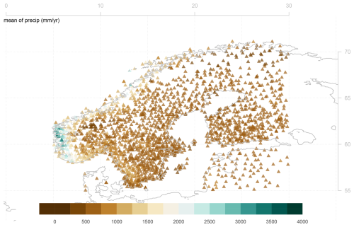
Figure 1Map showing the rain gauge station network from ECA&D used as predictands in the empirical–statistical downscaling of 24 h precipitation statistics. The colour legend shows the mean annual total precipitation.
The GCM data were taken from CMIP6 (Eyring et al., 2016) for historical runs (HIST) as well as various emission shared socio-economic pathway scenarios (SSP370, SSP126, SSP245, and SSP585) described in IPCC (2021). Only a subset of GCM runs was included here as daily precipitation was needed to estimate annual fw and μ for use as predictors. To reduce the data transfer amount, server-side data processing facilities at the German Climate Computing Centre (DKRZ) were used to derive the annual values with the Climate Data Operators (CDO) software (Schulzweida, 2021) installed on site. Nevertheless, a great deal of effort was required to derive fw and μ from ERA5 and all CMIP6 runs, and hence we make a case for a standard protocol for reanalysis and CMIP data archives that includes monthly fw and μ. The predictors, fw and μ, from CMIP6 HIST simulations were evaluated against ERA5 following Benestad et al. (2023), testing the GCMs' ability to reproduce the mean seasonal cycle, interannual variability in annual fw and μ, and their historical trends (see Appendix B). One simulation (CESM2-WACCM-FV2) was removed due to poor evaluation results, and our analysis focused on 29 model runs following SSP370, but the other emission scenarios are included in the Supplement (Benestad, 2024).
2.2 Downscaling methodology
An introduction to downscaling and its traditional definitions can be found in text books such as Benestad et al. (2008) and Maraun and Widmann (2018) and in shorter articles in scientific encyclopedias (Benestad, 2016). Our analysis introduces a new aspect in terms of downscaling using large-scale wet-day mean precipitation, μ, as predictors for estimating the predictand consisting of station-level μ, as well as using large-scale wet-day frequency, fw, as predictors to downscale local fw at the station level. Both of these types of predictors were estimated from the ERA5 reanalysis and CMIP6 GCMs for the Nordic region (55–72° N, 5° W–45° E) using common empirical orthogonal functions (henceforth “common EOFs”) as a framework for representing both the real-world and modelled conditions (Benestad, 2001). This choice implied using a so-called hybrid perfect prognosis model output statistics (PP-MOS, https://cordex.org/wp-content/uploads/2022/08/White-Paper-ESD.pdf, last access: 22 December 2024) framework to represent the predictors and ensured that the covariance structures from ERA5 used for calibration matched those from GCMs used for projection. The introduction of the ERA5 reanalysis has been a step change in terms of progress within ESD as there was a close match between fw and μ from the reanalysis and rain gauge measurements, respectively (see the Appendix B), enabling their use as predictors. More details and explanations about downscaling in general and the specific downscaling setup and analysis in our case are provided in Appendix A.
Here we distinguish between empirical orthogonal functions (EOFs) and principal component analysis (PCA). We used the former for data organized on a regular longitude–latitude grid, as is the normal convention in the scientific literature (Lorenz, 1956; Wallace and Dickinson, 1972; North et al., 1982; Preisendorfer, 1988; Navarra and Simoncini, 2010), whereas PCA (Wilks, 2006) was used for data series that had an irregular spatial distribution, such as rain gauge measurements. Moreover, we used PCA to represent the predictands as it tends to emphasize large-scale structures in groups of local measurements (Benestad et al., 2015a), and a step-wise multiple ordinary linear regression (OLR) was used to find an optimal connection between principal components from EOFs representing the large-scale predictors and the principal components from PCA representing local fw and μ. The downscaled annual fw and μ were subsequently used to estimate the probability that the daily precipitation amount (X′) exceeded a given threshold (x′) using the simple and approximate relation Pr based on Benestad et al. (2019). The analysis for daily precipitation amounts was extended to sub-daily timescales where the shape of intensity–duration–frequency (IDF) curves was downscaled based on their dependency on , where α was a calibrated adjustment factor, L was the duration of wet-spells in hours, τ was the return period, and ζ described the fractal dimension for temporal-scale inter-dependencies (Benestad et al., 2020). The downscaling was carried out using the R package esd (Benestad et al., 2015b), and the downscaled results for the sites of the rain gauge measurements were subsequently gridded through the kriging of the spatial weights with elevation as a co-variable using the R package LatticeKrig (Nychka et al., 2016). The kriging was applied to the spatial weights for the respective leading modes of PCA, which describe coherent geographical patterns of variability over the Nordic region. More details about the kriging method are provided in Appendix A.
2.3 Evaluation
The evaluation of the models and methods is documented in Appendix B and was applied to downscaled results through both conventional cross-validation and standard statistical tests of whether the observations belonged to the same statistical population as the downscaled multi-model ensemble. There was a close match between the aggregated rain gauge data and ERA5 for both fw and μ, where the cross-validation was 0.93 for the leading PCA mode for annual fw and where this leading PCA mode accounted for 50 % of the variance. The downscaling exercise for the second PCA (29 % of the variance) gave a cross-validation correlation of 0.92. Furthermore, the geographical weights of the calibrated ERA5 predictor matched spatial patterns of the corresponding PCA mode, as should be expected when the same variable is used as both the predictor and the predictand. Similarly, the downscaling exercise between aggregated rain gauge and ERA5 for annual μ returned cross-validation correlations of 0.96 and 0.81 for first and second PCA modes, respectively (representing 54 % and 26 % of the variance, respectively), also with matching spatial weights between calibrated ERA5 data and PCA modes. In summary, both high cross-validation correlation and similar geographical distribution of spatial weights in the predictors and predictands indicate a good match between the ERA5 and rain gauge measurement annual precipitation statistics when both involve the same variable.
It is important that the GCMs skilfully reproduce the same large-scale information that was found in the ERA5 reanalysis during calibration since we use it as a predictor when making projections for the future. Hence, our evaluation also involved testing the ability of the GCMs in reproducing the predictors in a skilful way and is described in more detail in Appendix B. The test of simulated predictor quality used common EOFs (Barnett, 1999) to compare the spatio-temporal covariance structure captured by simulations with corresponding information derived from the ERA5 reanalysis as in Benestad et al. (2023) but applied to fw and μ, respectively. The CMIP6 GCMs reproduced the mean seasonal cycle in fw and μ aggregated from the ERA5 reanalysis as well as the historical interannual mean variability in the annual fw and μ (for the period 1959–2021). A comparison of historical trends in GCM historical runs and ERA5 further indicated that the GCMs were able to reproduce the observed historical changes in fw and μ. The CMIP6 ensembles for fw and μ were of limited size since they were generated from daily data, and, for example, monthly fw and μ values are not (yet) part of the CMIP standard output protocol. We thus limited our analysis to one particular configuration from each GCM (e.g. r1i1p1f1). The number of ensemble members of regional or local climate projections can be interpreted as equivalent to statistical sample size as each model simulation involves non-deterministic stochastic decadal variability (Deser et al., 2012, 2020). The normal distribution may provide useful information on statistical data samples with about 30 data points if the data are normally distributed, and hence, distributions of downscaled ensemble results were tested against a normal distribution as in Benestad et al. (2023). The results of these tests suggested that the ensemble mean and standard deviation can provide an approximate description of the ensemble.
The evaluation of both the downscaling method and the GCM simulations established that local wet-day frequency, fw, and wet-day mean precipitation, μ, can be skilfully estimated over the Nordic region from corresponding large-scale quantities from both the ERA5 reanalysis and CMIP6 simulations. The subsequent step was to use these results to make projections for future climatic outlooks and estimate changes in precipitation statistics based on relationships established from previous studies (Benestad et al., 2019, 2020). Such steps are, to the best of our knowledge, the first efforts to downscale statistical properties for daily precipitation directly beyond downscaling extreme climate indices (Goodess et al., 2003; Haylock et al., 2006). Benestad et al. (2019) provided an evaluation of the statistical framework for estimating probabilities of moderate 24 h precipitation, which involved 1875 rain gauge records from North America and Europe with more than 50 years of valid data over the period from 1961–2018, and this evaluation will not be repeated here. To compensate for the thin upper tail of the exponential distribution, which is expected to significantly underestimate extremes, an empirical scaling factor, α, was introduced, and the analysis was restrained to moderate extremes (20–50 mm d−1). This scaling factor partly compensates for the fact that extreme 24 h precipitation does not follow an exponential distribution but has a thicker upper tail of the statistical distribution (Ye et al., 2018; Papalexiou and Koutsoyiannis, 2013).
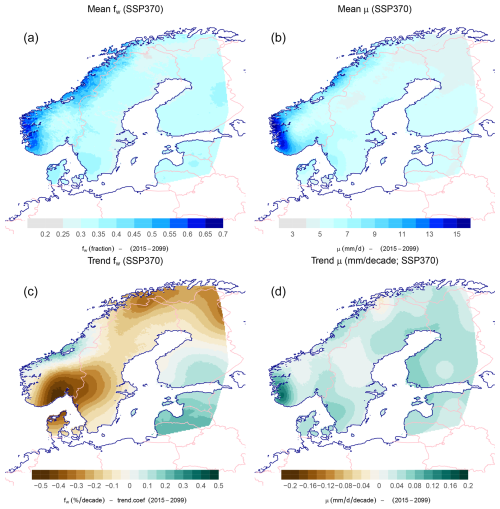
Figure 2 shows time series for the wet-day frequency, fw, and wet-day mean precipitation, μ, extracted for Blindern, Oslo, and the black symbols show the annual statistics derived from historical measurements, whereas the green band shows corresponding statistics downscaled from the CMIP6 SSP370 multi-model ensemble. The comparison between model results (green band) and observations (black symbols) gives an indication of the precision of the downscaling as it did not involve any further calibration beyond the original training of the downscaling model against the PCA-based predictand. Neither the observations nor the projections indicated any pronounced trend in the annual fw for Oslo; however, statistics based on rain gauge measurements over all the Nordic sites nevertheless suggested a general weak increase in the number of wet days over the 1950–2021 period that was statistically significant at the 5 % level (see the Supplement). The downscaled projections for Oslo (green shading in Fig. 2) and the Nordic countries (lower-left panel in Fig. 3), however, indicated a weak (geographically mixed and non-significant) general decrease in the number of wet days for the period 2015–2099 based on the ensemble mean of the CMIP6 simulations following the SSP370 emission scenario. Other emission scenarios gave some variations in the outlook, and SSP126 as well as SSP585 results gave a more mixed picture of trends in future fw (see the Supplement). The trend estimates in fw were expected to vary with the frequency of weather types, and the forces driving the atmospheric circulation that characterize different weather types tend to arise from variations in the distribution of atmospheric mass, which is not necessarily strongly constrained by an increased greenhouse effect. However, there has been as slight trend in annual fw in Oslo that was reproduced in a downscaling exercise using ERA5 as predictor (see the Supplement).
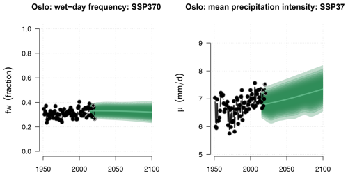
Figure 2Ensembles of downscaled wet-day frequency, fw, and wet-day mean precipitation, μ, for Oslo based on the SSP370 emission scenario. Black symbols show annual such aggregated statistics estimated from rain gauge measurements from Blindern, Oslo, and the green shading marks the ensemble spread of corresponding downscaled results.
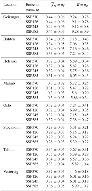
There has been a modest increase in annual wet-day mean precipitation, μ, that was more pronounced than the trends in fw, which is also visible in Fig. 2 (right panel) and Fig. 3d. The trend estimates in μ were more spatially consistent within the various emission scenarios, although higher emissions were connected to stronger trends, and the results indicated increases for most of the region except in the vicinity of Tromsø municipality in northern Norway. Table 1 presents the ensemble mean and standard deviation for a small selection of locations projected for the period from 2071–2100. The downscaled results suggested that projected trends in fw were not sensitive to the emission scenario (SSPs); however, the magnitude of projected trends in μ ranked from the lowest in SSP126, then SSP245 and SSP370, and the highest in SSP585.
Table 1The ensemble mean and standard deviation of the wet-day frequency, fw, and wet-day mean precipitation, μ, projected for 2071–2100 for a selection of locations.
Since the mean precipitation is the product of the wet-day frequency and wet-day mean precipitation4, we estimated trends in total precipitation based on the fw, μ, and product rule and used this information to explain total precipitation changes in terms of the changing number of wet days or changing intensity. Figure 4 shows estimated future trends in precipitation (mm d−1 per decade in upper panel; ) as well as its contribution regarding the changing number of wet days (lower left) and changes in mean precipitation intensity (lower right). The projections of the future climate in the Nordic region indicated a general increase in the total precipitation is mainly due to increased wet-day mean precipitation, μ, and in spite of decreased wet-day frequency, fw, according to the selected CMIP6 simulations.
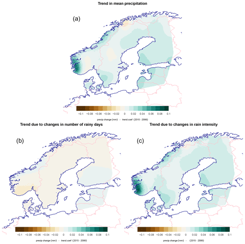
Figure 4Estimated trend in mean precipitation, (a), and the contribution due to wet days, fw, (c) and mean intensity, μ (d).
The wet-day frequency, fw, and wet-day mean precipitation, μ, represent two key parameters for approximate estimation of the probability of heavy rainfall according to
proposed and evaluated by Benestad et al. (2019). Figure 5 shows the observed fraction of days per year with more than 30 mm for Blindern, Oslo (black symbols), compared with such low-precision estimates based on this expression and the ensemble means for fw and μ (using the expression ; solid red line) shown with error bars of 1 standard deviation (dashed red). In other words, the results presented here were the downscaled estimates for fw and μ used as input in Eq. (1) without further calibration, and the statistics based on rain gauge measurements and information downscaled from the GCM ensembles indicated somewhat matching levels; however, the observations included some years with substantially higher numbers of days with heavy rainfall. These results nevertheless serve as an example where probabilities for heavy rainfall have been downscaled directly though the parameters fw and μ as opposed to aggregating data points from of a statistical sample containing traditionally downscaled time sequences of weather states. Another benefit with a parameterized expression for probability was that we could differentiate it according to the product rule as follows: . Figure 6 shows maps of both Pr and percentage trends5 for the SSP370 ensemble mean, and the results indicated the highest probabilities for days, receiving more than 30 mm of precipitation on the west coast of Norway, but the relative trends were the greatest over northern Finland. The density of rain gauge measurements was lower in northern Finland and Norway, however, and the uncertainties there are expected to be higher than further south (see Appendix A for further details).
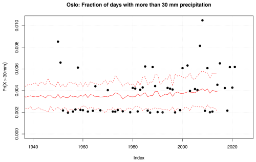
Figure 5Observed and estimated fraction of days per year in Oslo with more than 30 mm based on Eq. (1). The solid line shows estimates using the ensemble mean for fw and μ as input and dashed lines the ensemble mean with the ensemble standard deviation added or subtracted. The red curves represent the raw results of the calculation and do not involve any further calibration.
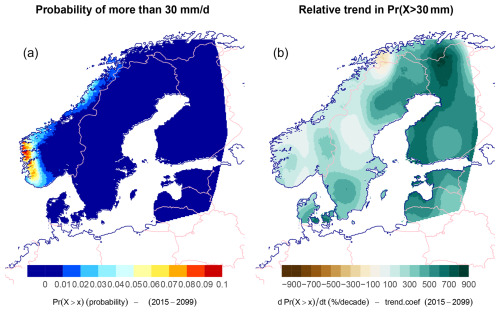
Figure 6Estimates of the mean probability of more than 30 mm precipitation in 24 h according to Pr (a) and the proportional trend in the probability estimated using the product rule (b). These results are based on downscaled fw and μ from the CMIP6 ensemble following the SSP370 emission scenario.
The parameterized expression for probabilities also enabled the downscaling of approximate estimates of return values based on , where α is a calibration coefficient (Benestad et al., 2019). Figure 7 shows both 10-year (left panels) and 25-year (right panels) return values as well as their estimated trends (lower panels) based on the ensemble mean SSP370 results. The greatest return values were estimated over western Norway, with 10-year estimates ranging within 30–170 mm d−1, while 25-year estimates varied within the range 40–220 mm d−1. The lowest estimates were downscaled for parts of northern Finland, Sweden, and Norway. Projected future trends in were estimated based on trends in the wet-day frequency, , and wet-day mean precipitation, (lower panels in Fig. 3); the above expression; and the product rule, and increases in were in general a result of increasing mean intensity rather than more wet days. The greatest trends in the return value, , were downscaled over western Norway with already high levels, but there were also notable increases over southwestern Finland and over parts of southwestern Sweden.
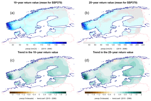
Figure 7Estimates of the 10-year and 25-year return values based on the expression (Benestad et al., 2019) and their future trend estimates (c, d). The results are based on the SSP370 emission scenario and the CMIP6 ensemble mean downscaled fw and μ (a, b).
Downscaled fw and μ also provided first-guess estimates for intensity–duration–frequency (IDF) curves, assuming there is a fractional dependence between temporal scales. We based our estimates of IDFs on Benestad et al. (2020) using the expression , which describes mathematical curves whose shapes are approximately similar to IDF curves estimated through more traditional means, where α is the same calibration coefficient as above, L is the duration in hours, τ is the return interval, and ζ describes the fractional dependency between temporal scales and was fitted to observational rain gauge measurement data. We estimated how the shape of IDF curves may change due to trends in fw and μ (their trends are shown in the lower panels in Fig. 3), and IDFs for Oslo for the present and the future are shown in Fig. 8. Different estimates for IDFs for the present, , and the future, , provide an opportunity to estimate scaling factors for IDF and curves to account for further climate change: 1.13–1.14 for fw and μ projected with SSP370 ensemble mean, not taking into account decadal variability. A crude measure for accounting for decadal variability was to use the ensemble spread ± σ, and subtracting σ for the present and adding σ in the future gave scaling factors within the range of 1.18–1.20 for SSP370. For higher emissions associated with SSP585, the scaling factors were 1.27–1.38 and in this case only based on the ensemble mean and not accounting for decadal variability. All these estimates varied with the return period τ, but the scaling factors were the same across time duration L in accordance with the expression above. In this case, we assumed that α and ζ were constant for a given site.
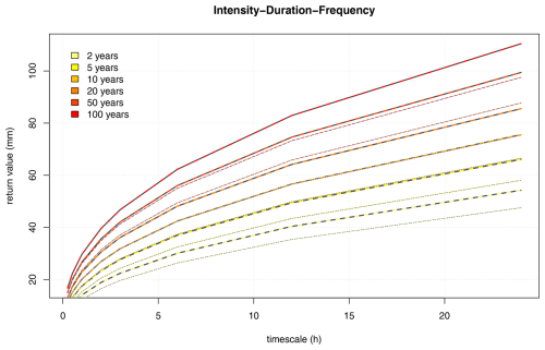
Figure 8Estimate of intensity–duration–frequency curves for Blindern, Oslo, based on downscaled fw and μ (thin solid–dotted) and their future trend estimates (thick solid–dashed). These results are based on the SSP370 emission scenario and the expression (Benestad et al., 2020).
We also explored the connection between the wet-day frequency and duration of dry spells (number of consecutive dry days), which may provide some indication of meteorological drought risk (see the Supplement). The calibration of our ESD method indicated that there was a link between large-scale fw values from ERA5 and the mean duration of dry spells. The spell duration approximately followed a geometric distribution where the mean duration (number of consecutive dry days) was the inverse of the success probability, which implies that we can approximately estimate the probability of a dry spell lasting longer than a given threshold. A projected weak reduction in fw over the Nordic region will therefore suggest slightly increased risks of meteorological droughts in the future.
To our knowledge, this is the first time the shape of curves representing probabilities for heavy rainfall or IDF curves has been downscaled using a hybrid PP-MOS approach (which addresses the “domain adaption” aspect discussed in Rampal et al., 2024) applied to multi-model GCM ensembles, albeit estimating the parameters defining their shapes. Those parametric expressions nevertheless enabled us to analyse the causes for trends in precipitation, probabilities, return values, probability of meteorological droughts, or shifts in the shape of IDF curves. These statistics were calculated from formulas which used downscaled fw and μ as input, and the results underscored that both the wet-day frequency and the wet-day mean precipitation are two key parameters for describing 24 h precipitation. In our case, the results were more sensitive to the mean precipitation intensity, μ, than wet-day frequency, fw.
Our results suggested a slight reduction in the future wet-day frequency over the Nordic countries, which may reflect predominant changes in the atmospheric circulation patterns due to the location of storm tracks and blocking high-pressure systems. Present state-of-the-art GCMs still have biases when it comes to storm tracks and blocking frequencies, which is possibly due to a coarse representation of the polar jet stream and other processes in the Arctic (IPCC, 2021). The downscaling may underestimate long-term changes in the mean precipitation intensity μ, even if the evaluation of the CMIP6 models seemed to score well on the comparison between trends in GCMs and ERA5. A separate test where μ was downscaled solely based on ERA5 reanalysis did not capture the historical changes observed in Oslo (see the Supplement). Furthermore, the projections of the wet-day frequency, fw, did not account for the risk that circulation patterns may change in ways not captured by present models. There may also be tipping points in the North Atlantic and sea ice cover, changes in the jet stream, effects from displaced storm tracks, and inaccurate simulation of blocking high-pressure system frequencies (IPCC, 2021). Nevertheless, a take-home message is that long-term trends in μ were sensitive to future emissions.
One question is whether the fractal temporal scaling properties utilized in the approximate IDF representation in Fig. 8 are stable or if we can expect them to change in time and space. It is also possible that there are diverging trends in fw or μ during different seasons that cancel each other out in the annual mean that are, for example, associated by prevailing presence of different seasonal meteorological phenomena. Our results suggested that the annual wet-day frequency, fw, was more coherent over space as all the 20 leading EOFs combined accounted for 88 % of the variance in the ERA5 reanalysis compared to 74 % for the annual wet-day mean precipitation, μ. Moreover, the leading EOF mode for the annual wet-day mean precipitation, μ, from ERA5 captured 19 % of the variance as opposed to 30 % for fw, which suggests that μ to a greater degree reflects small-scale processes and phenomena not being as strongly correlated over the region on annual timescales. Local and mesoscale processes and phenomena that may influence μ include surface-air fluxes, and local geographical effects such as orographic forcing. However, both fw and μ are expected to reflect meteorological phenomena ranging from local microscale to mesoscale and synoptic scales that may produce precipitation with different characteristics, dynamics and mechanisms, including convection, cut-off lows, mid-latitude cyclones, frontal systems, atmospheric rivers, and orographic forcing. Both increased precipitation amount from higher surface temperature and changes in the distribution of the precipitation over the planetary surface play a role in the trends in extreme precipitation amounts. Benestad et al. (2024) found a link between increased intensity on the one hand and increased rate of evaporation as well as changes in the global surface area receiving daily precipitation on the other. They also observed that changes in the global fractional surface area with daily precipitation were connected to the global statistics of the wet-day frequency, fw.
It is important to combine equivalent results from both ESD and RCMs when downscaling is used to produce regional or local climate projections for the future since they are based on different assumptions and have different strengths and weaknesses but are expected to give similar results for aggregated precipitation and temperature. All expressions used here in connection with ESD can also be combined with RCMs as Oguz et al. (2024) used the EURO-CORDEX ensemble (RCMs) rather than ESD to estimate fw and μ. They subsequently used the IDF curves as a basis for weather generators (Monte Carlo simulations) to provide input for landslide modelling. We leave a comparison with similar information from RCMs for future work.
Our results were produced with a hybrid PP-MOS strategy for downscaling climatic parameters represented through PCAs that may serve as a benchmark for machine learning and artificial intelligence (AI; Rampal et al., 2024). There is value in combining this ESD approach with more advanced machine learning (ML) or artificial intelligence (AI) methods that produce results with very different constraints. However, since downscaling fw or μ does not require as large data volume or as long time series as either ML, AI, or traditional methods for studying extremes, such a comparison is limited to cases with ample observational data or “pseudo-realities” using model output. One merit of our strategy is that it provides an explainable method which enhances our understanding of projected changes and thus complements many ML/AI methods. Hence, our downscaling strategy addresses some of the research questions stated in Rampal et al. (2024), and when the recipe of the entire analysis can be documented through an R Markdown script (see the Supplement), it is easier to provide transparency and the traceability sought in scientific discourse.
It is important to account for chaotic and stochastic variability on regional and decadal scales (Deser et al., 2012, 2020), for instance, using large multi-model ensembles as a surrogate for statistical sampling and letting the ensemble spread give a crude representation of probable outcomes. This analysis suggested that the ensemble spread for both annual fw and μ was approximately normal which implies that the ensemble mean as well as the standard deviation may provide useful information about the ensemble spread. The CMIP ensemble here was limited to one simulation per GCM because fw and μ had to be estimated from available daily output, making it difficult to explore uncertainties connected to initial conditions, natural variability, and model choices (Mezghani et al., 2019). However, it may be possible to use factorial regression or ANOVA to assess how model choice affects the downscaled ensemble with larger multi-model ensembles that include multiple simulations with the same GCM (Benestad et al., 2017, 2016). With the available CMIP6 data in this case, it was only possible to carry out an assessment of the sensitivity to emissions through comparing downscaled results from SSP126, SSP245, SSP370, and SSP585.
We used the ERA5 reanalysis and local rain gauge measurements from Nordic countries to calibrate empirical–statistical downscaling models, which were applied to CMIP6 projections using annual wet-day frequency, fw, and wet-day mean precipitation, μ, respectively, as both predictors and predictands. A good match between the ERA5 reanalysis and rain gauge measurements for these two key statistics over the Nordic region made for a good calibration of our downscaling method. Predictors from global climate models from CMIP6 were evaluated and scored well in terms of their ability to represent mean seasonal variations, interannual variability of annual aggregates, and past trends of the large-scale predictors needed for the downscaling. Our downscaling used a hybrid PP-MOS approach for estimating parameters for mathematical curves providing actionable regional climate information. The downscaled fw and μ were subsequently used to estimate local probabilities for heavy rainfall, return values, and changes in the shape of intensity–duration–frequency curves. We used kriging with elevation as a covariate to generate Nordic maps of fw and μ and their projected changes. Projected changes in the future suggest increases in μ but very slight decreases in fw, hinting at less frequent or a similar level of wet days in the future but also more intense rainfall. The amplitude of projected trends in μ was sensitive to the emission scenario, but trends in fw were not. The spread between the ensemble members was approximately normally distributed, which implies that essential information about the ensemble may be captured through the ensemble mean and standard deviation.
A1 Interpretations of the concept of downscaling
There are different definitions of downscaling, one being the mapping of data onto a finer grid (https://doi.org/10.5194/egusphere-2024-1463-RC1, Anonymous Referee, 2024) and another for which the information on large-scale features, which climate models are able to reproduce, is combined with information about the dependency across spatial scales to derive small-scale information (Benestad, 2016). The former may not always take into account the fact that numerical models have a minimum skilful scale and only provide a limited representation of reality (Takayabu et al., 2015). Downscaling is not restricted to producing gridded data with a higher resolution, and there are examples where downscaling has been carried out for a single location (Wilby et al., 2002; Maraun et al., 2015; Benestad et al., 2008). Moreover, the main objective of the COST VALUE project (Maraun et al., 2015) was to establish a standard evaluation scheme based on 85 different single locations scattered across Europe. On the other hand, a plain interpolation to a finer grid is usually not considered to be a downscaling approach, but bias adjustment is sometimes referred to as downscaling. Neither an interpolation, spatial disaggregation, nor bias adjustment, or any combination thereof, emphasizes the large-scale aspects that numerical models are able to reproduce with greater skill than grid-point estimates.
Global climate models have a typical spatial resolution of 100 km and therefore only have a coarse representation of the land surface, and the mountain regions are represented by crude pixels with typically lower heights than in reality. Some of the said simple approaches for producing data on a finer grid may implicitly add information about elevation, for example, through the inclusion of bias adjustment or kriging with elevation as a covariate, but the models' minimum skilful scale is not the same as the model resolution. Moreover, it is acknowledged that the models' minimum skilful scale typically encompasses several grid boxes (Von Storch et al., 1993; Benestad, 2016). Various models in the CMIP6 ensemble have a different spatial resolution, ranging from 50 km to 260 km, whereas the ERA5 has a resolution of approximately 31 km (these data are provided on a reduced Gaussian grid which has quasi-uniform spacing over the globe). Furthermore, model data typically represent the average value over a grid-box volume (e.g. temperature) or area (e.g. precipitation) with a spatial dimension of several cubic or square kilometres, whereas observations represent conditions at spatial scales of metres. The local rain gauge data can, for all intents and purposes, be considered point-source measurements (collected by funnels with a 20 cm diameter) and represent local (small-scale) climate information. In our analysis, downscaling provides the translation of large-scale information that can be provided by global climate models to local statistics for precipitation collected by rain gauges by adding information about their dependencies.
While RCMs and traditional ESD provide output for a sequence of atmospheric states (or outcomes) at a daily or sub-daily resolution, which we can refer to as weather conditions, our strategy has been to downscale the key parameters describing the shape of the mathematical curve for local probability, rather than estimating the statistics from samples made up of such data sequences. We can loosely refer to the former as downscaling weather, whereas the latter can be termed downscaling climate if climate can be defined as weather statistics or probability density functions (PDFs) reflecting (sub-)daily precipitation amounts. The application of the downscaling climate approach is not as widespread as the downscaling of time sequences with individual atmospheric states. Statistical properties of precipitation are expected to follow a more systematic geographical distribution than any random individual weather event, being influenced by prevailing large-scale conditions as well as fixed local geographical factors. Our objective was to downscale parameters describing the shape of a PDF or similar mathematical curves, and this approach was first inspired by Pryor et al. (2005, 2006) and is based on a long-term effort and a series of projects – e.g. EU SPECS (https://cordis.europa.eu/project/id/308378, last access: 22 December 2024, CiXPAG (https://cicero.oslo.no/no/prosjekter/cixpag, last access: 22 December 2024, KlimaDigital (https://www.sintef.no/projectweb/klimadigital/, last access: 22 December 2024, and EU SPRINGS (https://www.springsproject.eu/, last access: 22 December 2024). The downscaling climate approach can also be applied to, for example, summertime heatwaves or used to downscale the probability of the occurrences, nH, as well as the duration of hot spells, (Benestad et al., 2018); however, heatwaves were beyond the scope of the present analysis. Another example of the merit of this concept is the downscaling of storm track density (Parding et al., 2019), and future work in the EU SPRINGS project will explore the possibility of downscaling public health statistics for waterborne diseases that may lead to diarrhoea.
Using the same variables for predictors and predictands, as in this case, leaves it up to the GCMs to represent the underlying phenomena that generate precipitation. We could refer to this strategy as a hybrid super-resolution model output statistics (SR-MOS) in the terms proposed by Rampal et al. (2024) rather than PP-MOS; however, we stick to PP-MOS for simplicity. Improved GCMs in the future may reproduce various meteorological phenomena and processes with improved skill, which may lead to better estimates for future projections. It is also important that the reanalysis used for calibration matches the predictands closely.
A2 The predictors representing the large scales
Both the covariates from reanalyses used for calibrating the downscaling methods and corresponding covariates from global climate models used for making projections are referred to as predictors in the context of downscaling. Such predictors represent large-scale aspects that global climate models are able to reproduce with skill. Here we chose predictors that consisted of the same variables as the small-scale information that we sought through downscaling: the annual wet-day frequency, fw, and the annual wet-day mean precipitation, μ. This choice was motivated by the expectation of a systematic dependency between the large-scale and small-scale aspects of the same variable.
All of the CMIP6 models in our analysis were regridded to match the grid of ERA5 for the region (55–72° N, 5° W–45° E). Since data produced by reanalyses and global climate models have a high degree of redundancy, the information contained therein can be reorganized as spatially coherent patterns which represent substantial fractions of the covariance structure. These patterns involve mathematical techniques within linear algebra (Strang, 1988) known as empirical orthogonal functions (Lorenz, 1956; Wallace and Dickinson, 1972; North et al., 1982; Preisendorfer, 1988; Navarra and Simoncini, 2010), commonly referred to as EOFs. EOFs (and PCA used to describe predictands in the next subsection) make use of this redundancy and organize the information so that the most salient aspects of its covariance structure are represented by its leading modes. Furthermore, the high degree of redundancy makes it possible to represent the most important covariance information in a much smaller volume of data than the original raw data as illustrated by the schematic in Fig. A1. Here we use X to represent the anomalies of the original data with a temporal dimension, nt, and a spatial dimension, nr (for gridded data, , but here the particular geographical arrangement of the data points is not affecting the calculations). EOFs (and the PCA for the predictand) were implemented through the means of a singular value decomposition (SVD) (Strang, 1988), where U represented the spatial weights (“geographical pattern”), Λ was a diagonal matrix that held the eigenvalues (variances) in decreasing order, and V contained the time series (principal components, PCs, used in the regression analysis) according to
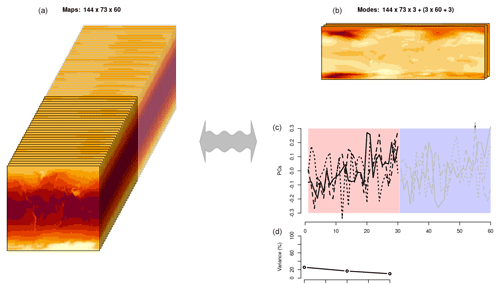
Figure A1A graphical illustration of representing the predictors in terms of EOFs. The left-hand side shows the data matrix with one map for each year, but since there are many reoccurring/similar (typical) spatial patterns, it is possible to represent the most salient information of these data matrix in terms of three dominant patterns (right-hand side), with temporal weights describing their presence and eigenvalues indicating their general prominence. This schematic furthermore illustrates the concept of common EOFs, where one part of the data matrix holds reanalysis data and another part holds GCM data. Their temporal weights are also distinguished by a different background colour on the right, and the part representing the reanalysis is then used in the calibration against rain gauge data, whereas the other part is used for making projections. Typically, the common EOFs require much less computer memory and are easier to process than the original data. They also provide a framework for evaluating the predictors since the temporal weights associated with the reanalysis and the GCM should have similar statistical properties. Since our schematic only includes the three leading modes, it reflects the expression X≈UΛVT rather than Eq. (A1).
One important issue is that the same large-scale structures in the predictors found for the reanalysis during calibration of the downscaling methods must be found in the model simulations to make projections for the future. A simple way to ensure identical covariance structures in the two is to use so-called common EOFs as proposed more than 20 years ago by Benestad (2001), where anomalies of the GCM data are mapped onto the same grid (regridded) as those from the reanalysis and the respective anomalies are combined so that the GCM data follow the ERA5 data in time; . Here, each GCM simulation was regridded to match the grid of ERA5 through bilinear interpolation, and ordinary EOFs were estimated for the joint data matrix. Since the spatial pattern, U, and the eigenvalue, Λ, were common for the joint data matrix, the two data sources were only distinguished by in Eq. (A1).
A3 The predictands representing the small scales
The predictand consisted of 652 local rain gauge measurements from the Nordic countries over the period from 1951–2021, and one reason to use a principal component analysis (PCA) of annually aggregated statistics (fw and μ) was that its gravest modes had a closer link to large-scale predictors than each local time series (Benestad et al., 2015a). The mathematics of PCA was similar to that of EOFs (Eq. A1), but the original data and hence the matrices therein were distinct from that of the predictor and can be expressed as . The difference between EOFs and PCA is that the former represents data on regular longitude–latitude grids, where the data are weighted by the area of their respective grid-box area, whereas PCA represents data with coordinates that have irregular structures. The downscaling only involved a representation of the predictands in the shape of PCA, where the local climate information was embedded in the spatial weight, U′, and eigenvalue, Λ′.
The local rainfall was measured at various locations with an irregular geographical spread, with some regions having more observations than others (Fig. 1), and there was a denser network of data in some regions (e.g. southern Scandinavia) and sparser network in others (e.g. the north). Regions with a different density of data get weighed differently with the PCA, and the results presented here involved a less effective calibration for areas with a lower station density (such as northern Norway/Finland) than southern Scandinavia. This caveat may imply higher uncertainties for the data-sparse regions in the far north.
The results from the downscaling were subsequently post-processed to provide maps as shown herein. The maps were generated though a kriging based on Markov random fields (Nychka et al., 2016) and made use of the R package LatticeKrig, which follows a fixed-rank kriging approach with a large number of basis functions. It was designed to provide spatial estimates that were comparable to standard families of covariance functions, and its Markov random field approach, combined with a basis function representation, was supposed to enable an implementation of different geometries. The kriging aspect here was merely used to provide spatial maps once local information had been derived for fw and μ for the locations of the rain gauge measurements, and the main objective here was to demonstrate how daily precipitation statistics can be derived through empirical–statistical downscaling and then be used for making local projections for a future climate. Furthermore, the kriging was only applied to the spatial patterns of the PCA for the leading mode, U′, to produce , and the expression was subsequently used to generate maps of fw and μ, with X′ representing either fw or μ. For downscaled estimates, the contents of V′ were replaced with the results of the regression model presented in the section below.
While the statistical parameters fw and μ were subject to downscaling, we sought solutions for expressing the probability Pr and return periods of heavy precipitation (moderate extremes, typically ) based on a modified exponential distribution. We used approximated estimates for the probability of heavy precipitation based on Pr and return values according to . Benestad et al. (2019) evaluated these expressions for 9817 locations in Europe and North America, and we do not repeat this evaluation here (the results are published in an open-access journal). The approach for estimating the parameters that determine the shape of intensity–duration–frequency (IDF) curves was evaluated by Parding et al. (2023) and Benestad et al. (2020) for sites in Norway, and these evaluations are not repeated here either (said papers are also in open-access journals). The main objective here was to show how parameters that specify the shape of mathematical curves for local precipitation statistics can be derived directly through empirical–statistical downscaling given that the curves themselves provide useful information.
A4 Details about the downscaling method
To ensure that the spatial covariance structure in ERA5 associated with variation in the rain gauge statistics is the same in the GCM, the regression analysis was carried out within a framework of the spatial patterns held in matrix U that are common for both reanalysis and model. The calibration involved a step-wise multiple ordinary linear regression (OLR), which only used part of the principal component, VERA5:
In Eq. (A2) the term VERA5,i is principal component i of the EOFs representing the predictor from ERA5 used for calibration, whereas represents the jth-order principal component from the PCA, representing the predictand and the aggregated statistics based on the local rain gauge data. In this case, V′ and VERA5,i were synchronized time series representing local and large-scale annual precipitation aggregates, respectively. It is Eq. (A2) that facilitates the transform from large to small scales and is referred to as the downscaling method, in this case involving a regression model, whereas the rest of the data processing provides the preparations, framing, and proper context for this analysis. The calibration provided estimates for the regression coefficient, βi, which were then used to make projections for the future according to
where U′ and Λ′ are the spatial weight and eigenvalue from the PCA representing the predictand and incorporates the results from Eq. (A2). In other words, we used Eq. (A3) together with the regression coefficients and the part of the common EOFs representing the global climate models () to make projections.
In our downscaling attempts over the Nordic region, we used the five leading PCA modes () to represent the most salient information of annual fw and μ estimated from the rain gauge measurements (the predictands), representing 100 % of the variance in the station-based statistics for both. To represent the predictors, we used the seven leading EOFs (), estimated for fw or μ from ERA5, in a step-wise multiple OLR to estimate each PCA mode for the predictand. In other words, the OLR was used to relate large-scale information from ERA5 to local information provided by the rain gauge data, and time series representing annual fw and μ were generated based on the regression coefficient, βi, and subsequently computed according to Eq. (A3).
The first step of the model calibration involved a 5-fold cross-validation (Gutiérrez et al., 2018), where the data were split into five equal segments, and one was withheld from the calibration of the remaining four segments and then compared with predicted values (out of sample). This exercise was repeated for all combinations, and the final cross-validation scores were estimated based on all iterations. The final calibration, however, was carried out for annual data over the entire period from 1951–2021 (51 data points for each PCA mode).
B1 Cross-validation
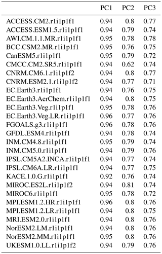
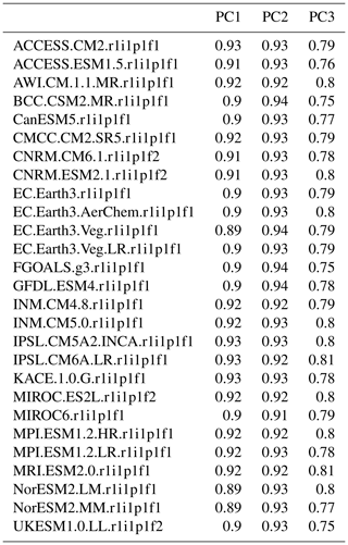
It is a standard practice to evaluate downscaled results through a cross-validation exercise and Tables B1–B2 show cross-validation correlations for each of the five PCA modes and for each type of GCMs. The scores vary slightly due to different spatial resolutions and slight differences in their embedded covariance information.
Table B1Cross-validation correlation of the principal components from PCA used to represent the predictand for fw (columns). The rows represent the different results for the different ensemble members.
B2 Evaluation of ERA5
A good match between annual rain gauge statistics and corresponding statistics derived from ERA5 also constitutes an evaluation of the ERA5 reanalysis. Hence, diagnostics of empirical–statistical downscaling can be used to evaluate reanalyses such as ERA5. Figure B1 gives a graphical representation of diagnostics associated with the calibration of the regression coefficients for the leading PCA mode, βi,1, of fw, where . These figures indicate that the spatial weights with the most impact on annual fw in ERA5 match the geographical distribution of the sites with the greatest weight in (upper panels show ), and the lower-left panel shows the results of a cross-validation applied to pure ERA5 data.
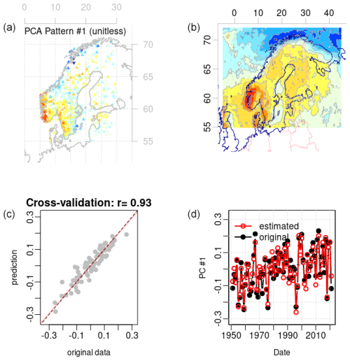
Figure B1Diagnostics of the calibration of the multiple regression model for the leading PCA mode for annual fw. Panel (a) shows the spatial weights of annual fw from derived from rain gauge measurements and panel (b) shows the spatial weights from the weighted combination of EOFs of corresponding ERA5 data weighted according to the regression coefficients from the calibration exercise. Panel (c) provides the results from a 5-fold cross-validation and (d) examines how well the multiple regression captures long-term trends. This is an example of a skilful calibration where the spatial weights match, the cross-validation score is high, and the long-term trends are well reproduced.
Figure B2 shows similar results for μ and shows that there was a close match between the annual wet-day mean precipitation aggregated from rain gauge data and the ERA5 reanalysis.
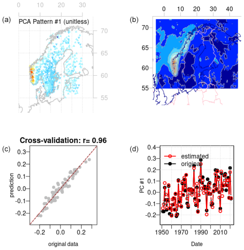
Figure B2Same as Fig. B1 but for μ.
B3 Evaluation of the global climate models
Since large-scale aspects were used as predictors in the downscaling, we evaluated the skill of the selected global climate models in reproducing them. Large-scale aspects from ERA5 were used for the calibration of the downscaling models, and therefore the climate simulations were compared with corresponding ERA5 data to make the evaluation relevant for the downscaling results. We started by assessing the mean annual cycle to provide a test of whether the representation of physical processes and conditions in the models captures the most salient variations such as the mean seasonal cycle. Further steps in our evaluation involved testing their ability to reproduce the characteristics of interannual variations and past trends in fw and μ. Both interannual variability and assessment of past trends are relevant for when downscaling is used to make projections for the future because the former reveals whether the models are able to reproduce the covariance information associated with the Earth's climate. It is also important that the models are able to capture changes (interannual variability and long-term trends) in the past if they are to be trusted to predict changes in the future. The results of these evaluations can be found in the Supplement but are not presented here in more detail as our main objective was to demonstrate how it is possible to downscale statistical properties on daily precipitation directly.
B4 Ensemble evaluation
An evaluation of downscaled ensemble results may include an assessment of whether the data follow a normal distribution, and rank statistics can be used to test whether the model results belong to the same statistical population as the observed target data. We tested the downscaled data in terms of both their rank statistics based on individual years and the ratio of observed to modelled standard deviations associated with their reproduction of interannual variability. It is important that the downscaled results reproduce the typical interannual variability and historical trends for the selected locations.
Figure B3 shows an evaluation of the statistical distribution of the downscaled ensemble results and suggests that the ensemble results were close to being normally distributed for both fw and μ. Hence, information about the ensemble can be approximated by the ensemble mean and ensemble standard deviation.
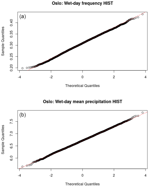
Figure B3A comparison between the ensemble distribution (historical run) and the normal distribution for annual fw (a) and μ (b) for their respective leading PCA. The near-linear fit suggests that the distribution of the ensemble results is close to being normally distributed for the most important PCA mode.
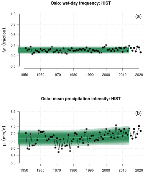
Figure B4A comparison between the downscaled ensemble annual fw (a) and μ (b) for Oslo and corresponding observations indicates that the model results reproduce both amplitude and long-term trends at a realistic level.
The average rank of annual respective fw and μ from the observations from Blindern, Oslo, was estimated over the 1951–2014 period in terms of the downscaled results (Fig. B4). If the ensemble results belonged to the same statistical population as the observations, then this rank statistics should follow a uniform distribution. For fw, the mean rank was 0.49 and well within the range of 0–1 (p value of 0.49). The observed standard deviation for fw was 1.33 times that of the ensemble for the overlapping historical simulations. Likewise, the mean rank for μ was 0.44, with a corresponding ratio in standard deviation of 1.41. Figure B4 shows the case, for Blindern, Oslo, as an example of how the downscaled ensemble can be assessed, and in this case the downscaled ensemble gave a slight underestimate of the magnitude of the interannual variability.
An evaluation of trends indicated ranges for both fw and μ which spanned the observed trends at the 652 locations, but the ensembles underestimated the interannual variability for both fw and μ (see the Supplement).
We have, in our analysis, explored annually aggregated fw and μ, but the presence of various meteorological phenomena tends to vary with the seasons, and a mean annual trend may mask possible opposite trends in different seasons. To assess this possibility, we took a random sample from historical rain gauge measurements from Oslo and compared seasonal trends in both fw and μ (see the Supplement). Our random test suggested that there were no pronounced opposite trends, but a more thorough exercise would entail downscaling seasonal mean precipitation statistics for the Nordic region. We leave the task of seasonal focus for the future as a part of our objectives was to develop and evaluate the downscaling approach for the EU SPRINGS project and to provide the first projections for the planned national report Klima i Norge 2100. This strategy will also be explored in collaboration with Mozambique through a CORDEX flagship pilot study (FPS) southeast Africa and the Norad-funded project Sarepta (https://bistand.met.no/en/Sarepta, last access: 23 December 2024). This downscaling climate approach for precipitation may work even if there is limited rain gauge data, but it is important that reanalyses such as ERA5 correspond well to data on the ground.
The R Markdown script, on which this analysis is based, is provided in the Supplement and available from figshare (https://doi.org/10.6084/m9.figshare.25809196.v2, Benestad, 2024).
The data used in the analysis are available together with computer code from FigShare at https://doi.org/10.6084/m9.figshare.25809196.v2 (Benestad, 2024).
The supplement related to this article is available online at: https://doi.org/10.5194/hess-29-45-2025-supplement.
REB conceptualized and carried out most of the analysis and drafted the paper; AD processed CMIP data and contributed to writing up the paper; KMP has contributed to method development within the R package esd and writing.
The contact author has declared that none of the authors has any competing interests.
The future projections are only as good as the GCMs on which they are based. They are the best information we have at the time of this analysis and are based on various assumptions, and there is always a risk that factors unaccounted for also play a role and may result in a different future climatic evolution.
Publisher’s note: Copernicus Publications remains neutral with regard to jurisdictional claims made in the text, published maps, institutional affiliations, or any other geographical representation in this paper. While Copernicus Publications makes every effort to include appropriate place names, the final responsibility lies with the authors.
The downscaling model and part of the analysis used the ECMWF fifth-generation ERA5 reanalysis hourly data downloaded from Copernicus C3S. We acknowledge the data providers in the ECA&D project by Klein Tank et al. (2002). Data and metadata are available at https://www.ecad.eu (last access: 23 December 2024). We acknowledge the CMIP6 community for providing the climate model data, retained and globally distributed in the framework of the Earth System Grid Federation (ESGF). The CMIP6 data and server-side computing resources for this study were made available by the German Climate Computing Centre (DKRZ) under project ID 1088.
This work was funded jointly by the following projects: EU SPRINGS (project no. 101137255 15 – HORIZON-HLTH-2023-ENVHLTH-02), Klima i Norge (MET Norway), Sarepta (Norad), and CORDEX ESD (in-kind).
This paper was edited by Louise Slater and reviewed by three anonymous referees.
Anonymous Referee: Referee Comment 1, Comment on egusphere-2024-1463, https://doi.org/10.5194/egusphere-2024-1463-RC1, 2024.
Barnett, T. P.: Comparison of Near-Surface Air Temperature Variability in 11 Coupled Global Climate Models, J. Climate, 12, 511–518, https://doi.org/10.1175/1520-0442(1999)012<0511:CONSAT>2.0.CO;2, 1999. a
Benestad, R.: Downscaling Climate Information, vol. 1, Oxford University Press, https://doi.org/10.1093/acrefore/9780190228620.013.27, 2016. a, b, c
Benestad, R.: Empirical-statistical downscaling of daily precipitation information in the Nordics, figshare [code and data set], https://doi.org/10.6084/m9.figshare.25809196.v2, 2024. a, b, c
Benestad, R., Sillmann, J., Thorarinsdottir, T. L., Guttorp, P., Mesquita, M. D. S., Tye, M. R., Uotila, P., Maule, C. F., Thejll, P., Drews, M., and Parding, K. M.: New vigour involving statisticians to overcome ensemble fatigue, Nat. Clim. Change, 7, 697–703, https://doi.org/10.1038/nclimate3393, 2017. a
Benestad, R. E.: A comparison between two empirical downscaling strategies, Int. J. Climatol., 21, 1645–1668, https://doi.org/10.1002/joc.703, 2001. a, b
Benestad, R. E.: A new global set of downscaled temperature scenarios, J. Climate, 24, 2080–2098, https://doi.org/10.1175/2010JCLI3687.1, 2011. a
Benestad, R. E., Hanssen-Bauer, I., and Chen, D.: Empirical-statistical downscaling, World Scientific, https://doi.org/10.1142/6908, 2008. a, b
Benestad, R. E., Chen, D., Mezghani, A., Fan, L., and Parding, K.: On using principal components to represent stations in empirical-statistical downscaling, Tellus A, 67, 28326, https://doi.org/10.3402/tellusa.v67.28326, 2015a. a, b
Benestad, R. E., Mezghani, A., and Parding, K. M.: esd V1.0, Zenodo, https://doi.org/10.5281/zenodo.29385, 2015b. a
Benestad, R. E., Senan, R., and Orsolini, Y.: The use of regression for assessing a seasonal forecast model experiment, Earth Syst. Dynam., 7, 851–861, https://doi.org/10.5194/esd-7-851-2016, 2016. a
Benestad, R. E., Oort, B. v., Justino, F., Stordal, F., Parding, K. M., Mezghani, A., Erlandsen, H. B., Sillmann, J., and Pereira-Flores, M. E.: Downscaling probability of long heatwaves based on seasonal mean daily maximum temperatures, Advances in Statistical Climatology, Meteorology and Oceanography, 4, 37–52, https://doi.org/10.5194/ascmo-4-37-2018, 2018. a
Benestad, R. E., Parding, K. M., Erlandsen, H. B., and Mezghani, A.: A simple equation to study changes in rainfall statistics, Environ. Res. Lett., 14, 084017, https://doi.org/10.1088/1748-9326/ab2bb2, 2019. a, b, c, d, e, f, g
Benestad, R. E., Lutz, J., Dyrrdal, A. V., Haugen, J. E., Parding, K. M., and Dobler, A.: Testing a simple formula for calculating approximate intensity-duration-frequency curves, Environ. Res. Lett., 16, 044009, https://doi.org/10.1088/1748-9326/abd4ab, 2020. a, b, c, d, e
Benestad, R. E., Mezghani, A., Lutz, J., Dobler, A., Parding, K. M., and Landgren, O. A.: Various ways of using empirical orthogonal functions for climate model evaluation, Geosci. Model Dev., 16, 2899–2913, https://doi.org/10.5194/gmd-16-2899-2023, 2023. a, b, c
Benestad, R. E., Lussana, C., and Dobler, A.: A link between the global surface area receiving daily precipitation, wet-day frequency and probability of extreme rainfall, Discover Water, 4, 10, https://doi.org/10.1007/s43832-024-00063-3, 2024. a
Christensen, J. H. and Christensen, O. B.: A summary of the PRUDENCE model projections of changes in European climate by the end of this century, Climatic Change, 81, 7–30, https://doi.org/10.1007/s10584-006-9210-7, 2007. a
Christensen, J. H., Carter, T. R., Rummukainen, M., and Amanatidis, G.: Evaluating the performance and utility of regional climate models: the PRUDENCE project, Climatic Change, 81, 1–6, https://doi.org/10.1007/s10584-006-9211-6, 2007. a
Coles, S. G.: An Introduction to Statistical Modeling of Extreme Values, Springer, London, ISBN 978-1-84996-874-4, 2001. a
Deser, C., Knutti, R., Solomon, S., and Phillips, A. S.: Communication of the role of natural variability in future North American climate, Nat. Clim. Change, 2, 775–779, https://doi.org/10.1038/nclimate1562, 2012. a, b, c
Deser, C., Lehner, F., Rodgers, K. B., Ault, T., Delworth, T. L., DiNezio, P. N., Fiore, A., Frankignoul, C., Fyfe, J. C., Horton, D. E., Kay, J. E., Knutti, R., Lovenduski, N. S., Marotzke, J., McKinnon, K. A., Minobe, S., Randerson, J., Screen, J. A., Simpson, I. R., and Ting, M.: Insights from Earth system model initial-condition large ensembles and future prospects, Nat. Clim. Change, 10, 277–286, https://doi.org/10.1038/s41558-020-0731-2, 2020. a, b, c
Eyring, V., Bony, S., Meehl, G. A., Senior, C. A., Stevens, B., Stouffer, R. J., and Taylor, K. E.: Overview of the Coupled Model Intercomparison Project Phase 6 (CMIP6) experimental design and organization, Geosci. Model Dev., 9, 1937–1958, https://doi.org/10.5194/gmd-9-1937-2016, 2016. a
Goodess, C., Osborn, T., and Hulme, M.: The identification and evaluation of suitable scenario development methods for the estimation of future probabilities of extreme weather events, Technical Report 4, Tyndall Centre, School of Environemtal Sciences, Univ. East Anglia, Norwich, https://www.researchgate.net/publication/267829957_The_identification_and_evaluation_of_suitable_scenario_development_methods_for_the_estimation_of_future_probabilities_of_extreme_weather_events (last access: 23 December 2024), 2003. a, b
Gutiérrez, J. M., Maraun, D., Widmann, M., Huth, R., Hertig, E., Benestad, R., Roessler, O., Wibig, J., Wilcke, R., Kotlarski, S., Martín, D. S., Herrera, S., Bedia, J., Casanueva, A., Manzanas, R., Iturbide, M., Vrac, M., Dubrovsky, M., Ribalaygua, J., Pórtoles, J., Räty, O., Räisänen, J., Hingray, B., Raynaud, D., Casado, M. J., Ramos, P., Zerenner, T., Turco, M., Bosshard, T., Štěpánek, P., Bartholy, J., Pongracz, R., Keller, D. E., Fischer, A. M., Cardoso, R. M., Soares, P. M. M., Czernecki, B., and Pagé, C.: An intercomparison of a large ensemble of statistical downscaling methods over Europe: Results from the VALUE perfect predictor cross‐validation experiment, Int. J. Climatol., 39, 3750–3785, https://doi.org/10.1002/joc.5462, 2018. a
Gutowski Jr., W. J., Giorgi, F., Timbal, B., Frigon, A., Jacob, D., Kang, H.-S., Raghavan, K., Lee, B., Lennard, C., Nikulin, G., O'Rourke, E., Rixen, M., Solman, S., Stephenson, T., and Tangang, F.: WCRP COordinated Regional Downscaling EXperiment (CORDEX): a diagnostic MIP for CMIP6, Geosci. Model Dev., 9, 4087–4095, https://doi.org/10.5194/gmd-9-4087-2016, 2016. a
Hawkins, E. and Sutton, R.: The potential to narrow uncertainty in regional climate predictions, B. Am. Meteorol. Soc., 90, 1095, https://doi.org/10.1175/2009BAMS2607.1, 2009. a
Haylock, M. R., Cawley, G. C., Harpham, C., Wilby, R. L., and Goodess, C. M.: Downscaling Heavy Precipitation Over the United Kingdom: A Comparison of Dynamical and Statistical Methods and their Future Scenarios, Int. J. Climatol., 26, 1397–1416, 2006. a, b
Hersbach, H., Bell, B., Berrisford, P., Hirahara, S., Horanyi, A., Munoz‐Sabater, J., Nicolas, J., Peubey, C., Radu, R., Schepers, D., Simmons, A., Soci, C., Abdalla, S., Abellan, X., Balsamo, G., Bechtold, P., Biavati, G., Bidlot, J., Bonavita, M., Chiara, G., Dahlgren, P., Dee, D., Diamantakis, M., Dragani, R., Flemming, J., Forbes, R., Fuentes, M., Geer, A., Haimberger, L., Healy, S., Hogan, R. J., Holm, E., Janiskova, M., Keeley, S., Laloyaux, P., Lopez, P., Lupu, C., Radnoti, G., Rosnay, P., Rozum, I., Vamborg, F., Villaume, S., and Thepaut, J.: The ERA5 global reanalysis, Q. J. Roy. Meteor. Soc., 146, 1999–2049, https://doi.org/10.1002/qj.3803, 2020. a
IPCC: Climate Change 2021: The Physical Science Basis. Contribution of Working Group I to the Sixth Assessment Report of the Intergovernmental Panel on Climate Change, Tech. rep., Cambridge University Press, https://doi.org/10.1017/9781009157896, 2021. a, b, c, d
Jacob, D., Teichmann, C., Sobolowski, S., Katragkou, E., Anders, I., Belda, M., Benestad, R., Boberg, F., Buonomo, E., Cardoso, R. M., Casanueva, A., Christensen, O. B., Christensen, J. H., Coppola, E., De Cruz, L., Davin, E. L., Dobler, A., Domínguez, M., Fealy, R., Fernandez, J., Gaertner, M. A., García-Díez, M., Giorgi, F., Gobiet, A., Goergen, K., Gómez-Navarro, J. J., Alemán, J. J. G., Gutiérrez, C., Gutiérrez, J. M., Güttler, I., Haensler, A., Halenka, T., Jerez, S., Jiménez-Guerrero, P., Jones, R. G., Keuler, K., Kjellström, E., Knist, S., Kotlarski, S., Maraun, D., van Meijgaard, E., Mercogliano, P., Montávez, J. P., Navarra, A., Nikulin, G., de Noblet-Ducoudré, N., Panitz, H.-J., Pfeifer, S., Piazza, M., Pichelli, E., Pietikäinen, J.-P., Prein, A. F., Preuschmann, S., Rechid, D., Rockel, B., Romera, R., Sánchez, E., Sieck, K., Soares, P. M. M., Somot, S., Srnec, L., Sørland, S. L., Termonia, P., Truhetz, H., Vautard, R., Warrach-Sagi, K., and Wulfmeyer, V.: Regional climate downscaling over Europe: perspectives from the EURO-CORDEX community, Reg. Environ. Change, 20, 51, https://doi.org/10.1007/s10113-020-01606-9, 2020. a
Klein Tank, A. J. B. W., Konnen, G. P., Böhm, R., Demarée, G., Gocheva, A., Mileta, M., Pashiardis, S., Hejkrlik, L., Kern-Hansen, C., Heino, R., Bessemoulin, P., Müller-Westermeier, G., Tzanakou, M., Szalai, S., Pálsdóttir, T., Fitzgerald, D., Rubin, S., Capaldo, M., Maugeri, M., Leitass, A., Bukantis, A., Aberfeld, R., Engelen, A. F. V. v., Førland, E., Mietus, M., Coelho, F., Mares, C., Razuvaev, V., Nieplova, E., Cegnar, T., López, J. A., Dahlström, B., Moberg, A., Kirchhofer, W., Ceylan, A., Pachaliuk, O., Alexander, L. V., and Petrovic, P.: Daily dataset of 20th-century surface air temperature and precipitation series for the European Climate Assessment, Int. J. Climatol., 22, 1441–1453, 2002. a, b
Lorenz, E. N.: Empirical Orthogonal Functions and Statistical Weather Prediction, Sci. rep. 1, Department of Meteorology, MIT, USA, Cambridge, Massachusetts, 1956. a, b
Lussana, C., Benestad, R., and Dobler, A.: Changes in regional daily precipitation intensity and spatial structure from global reanalyses, Int. J. Climatol., 44, 1135–1153, https://doi.org/10.1002/joc.8375, 2024. a
Maraun, D. and Widmann, M.: Statistical downscaling and bias correction for climate research, Cambridge University Press, https://doi.org/10.1017/9781107588783, 2018. a
Maraun, D., Widmann, M., Gutiérrez, J. M., Kotlarski, S., Chandler, R. E., Hertig, E., Wibig, J., Huth, R., and Wilcke, R. A.: VALUE: A framework to validate downscaling approaches for climate change studies, Earth's Future, 3, 2014EF000259, https://doi.org/10.1002/2014EF000259, 2015. a, b, c
Mezghani, A., Dobler, A., Haugen, J. E., Benestad, R. E., Parding, K. M., Piniewski, M., Kardel, I., and Kundzewicz, Z. W.: CHASE-PL Climate Projection dataset over Poland – bias adjustment of EURO-CORDEX simulations, Earth Syst. Sci. Data, 9, 905–925, https://doi.org/10.5194/essd-9-905-2017, 2017. a
Mezghani, A., Dobler, A., Benestad, R., Haugen, J. E., Parding, K. M., Piniewski, M., and Kundzewicz, Z. W.: Sub-sampling impact on the climate change signal over Poland based on simulations from statistical and dynamical downscaling, J. Appl. Meteorol. Clim., 58, 1061–1078, https://doi.org/10.1175/JAMC-D-18-0179.1, 2019. a
Navarra, A. and Simoncini, V.: A guide to empirical orthogonal functions for climate data analysis, Springer, Dordrecht, New York, ISBN 9789048137022, 2010. a, b
North, G. R., Bell, T. L., and Cahalan, R. F.: Sampling Errors in the Estimation of Empirical Orthogonal Functions, Mon. Weather Rev., 110, 699–706, 1982. a, b
Nychka, D., Hammerling, D., Sain, S., and Lenssen, N.: LatticeKrig: Multiresolution Kriging Based on Markov Random Fields, Boulder, CO, USA, https://doi.org/10.5065/D6HD7T1R, 2016. a, b
Oguz, E. A., Benestad, R. E., Parding, K. M., Depina, I., and Thakur, V.: Quantification of climate change impact on rainfall-induced shallow landslide susceptibility: a case study in central Norway, Georisk: Assessment and Management of Risk for Engineered Systems and Geohazards, 24 pp., https://doi.org/10.1080/17499518.2023.2283848, 2024. a
Papalexiou, S. M. and Koutsoyiannis, D.: Battle of extreme value distributions: A global survey on extreme daily rainfall: Survey on extreme daily rainfall, Water Resour. Res., 49, 187–201, https://doi.org/10.1029/2012WR012557, 2013. a
Parding, K. M., Benestad, R., Mezghani, A., and Erlandsen, H. B.: Statistical Projection of the North Atlantic Storm Tracks, J. Appl. Meteorol. Clim., 58, 1509–1522, https://doi.org/10.1175/JAMC-D-17-0348.1, 2019. a, b
Parding, K. M., Benestad, R. E., Dyrrdal, A. V., and Lutz, J.: A principal-component-based strategy for regionalisation of precipitation intensity–duration–frequency (IDF) statistics, Hydrol. Earth Syst. Sci., 27, 3719–3732, https://doi.org/10.5194/hess-27-3719-2023, 2023. a
Preisendorfer, R. W.: Principal Component Analysis in Meteorology and Oceanology, Elsevier Science Press, Amsterdam, ISBN 978-0444430144, 1988. a, b
Pryor, S., School, J. T., and Barthelmie, R. J.: Empirical downscaling of wind speed probability distributions, J. Geophys. Res., 110, D19109, https://doi.org/10.1029/2005JD005899, 2005. a
Pryor, S., School, J. T., and Barthelmie, R. J.: Winds of change? Projections of near-surface winds under climate change scenarios, Geophys. Res. Lett., 33, L11702, https://doi.org/10.1029/2006GL026000, 2006. a
Rampal, N., Hobeichi, S., Gibson, P. B., Baño-Medina, J., Abramowitz, G., Beucler, T., González-Abad, J., Chapman, W., Harder, P., and Gutiérrez, J. M.: Enhancing Regional Climate Downscaling through Advances in Machine Learning, Artificial Intelligence for the Earth Systems, 3, 230066, https://doi.org/10.1175/AIES-D-23-0066.1, 2024. a, b, c, d, e
Schulzweida, U.: CDO User Guide: Climate Data Operator, Version 2.0.0, October 2021, Tech. rep., MPI for Meteorology, https://code.mpimet.mpg.de/projects/cdo/embedded/cdo.pdf (last access: 24 December 2024), 2021. a
Strang, G.: Linear Algebra and its Application, Harcourt Brace & Company, San Diego, California, USA, ISBN 9780534422004, 1988. a, b
Takayabu, I., Kanamaru, H., Dairaku, K., Benestad, R., Storch, H. V., and Christensen, J. H.: Reconsidering the quality and utility of downscaling, J. Meteorol. Soc. Jpn., 94A, 31–45, https://doi.org/10.2151/jmsj.2015-042, 2015. a, b, c
Trenberth, K. E., Dai, A., Rasmussen, R. M., and Parsons, D. B.: The Changing Character of Precipitation, B. Am. Meteorol. Soc., 84, 1205–1218, https://doi.org/10.1175/BAMS-84-9-1205, 2003. a
Von Storch, H., Zorita, E., and Cubasch, U.: Downscaling of Global Climate Change Estimates to Regional Scales: An Application to Iberian Rainfall in Wintertime, J. Climate, 6, 1161–1171, https://doi.org/10.1175/1520-0442(1993)006<1161:DOGCCE>2.0.CO;2, 1993. a
Wallace, J. and Dickinson, R. E.: Empirical orthogonal representation of time series in the frequency domain: I. Theoretical considerations, J. Appl. Meteorol., 11, 887–892, https://doi.org/10.1175/1520-0450(1972)011<0887:EOROTS>2.0.CO;2, 1972. a, b
Wilby, R., Dawson, C., and Barrow, E.: sdsm – a decision support tool for the assessment of regional climate change impacts, Environ. Modell. Softw., 17, 145–157, https://doi.org/10.1016/S1364-8152(01)00060-3, 2002. a
Wilks, D. S.: Statistical methods in the atmospheric sciences, vol. 91, International Geophysics Series, Academic Press, Amsterdam, Boston, 2nd edn., ISBN 978-0-12-751966-1, 2006. a
Ye, L., Hanson, L. S., Ding, P., Wang, D., and Vogel, R. M.: The probability distribution of daily precipitation at the point and catchment scales in the United States, Hydrol. Earth Syst. Sci., 22, 6519–6531, https://doi.org/10.5194/hess-22-6519-2018, 2018. a
Henceforth, we use the term GCM when referring to both GCMs and ESMs.
There are, however, empirical–statistical downscaling (ESD) methods that are closer to bias correction, downscaling grid points separately and hence not taking minimum skilful scale into consideration. For example, NASA's NEX-GDDP data set (https://www.nccs.nasa.gov/services/data-collections/land-based-products/nex-gddp, last access: 22 December 2024) is presented as downscaled climate scenarios but the method is a type of bias correction. Also see Appendix A for further discussion on this topic.
This refers to how closely we can reproduce the shape of the mathematical curve describing probabilities rather than a bias/variance issues for the predicted outcomes.
, where and .
The trend is .
- Abstract
- Introduction
- Data and methods
- Results
- Discussions
- Conclusions
- Appendix A: Detailed information about the downscaling methodology
- Appendix B: Evaluation
- Appendix C: Projections of regional future precipitation statistics
- Code availability
- Data availability
- Author contributions
- Competing interests
- Disclaimer
- Acknowledgements
- Financial support
- Review statement
- References
- Supplement


