Constraining topsoil pesticide degradation in a conceptual distributed catchment model with compound-specific isotope analysis (CSIA)

Predicting pesticide dissipation at the catchment scale using hydrological models is challenging due to limited field data distinguishing degradative from non-degradative processes. This limitation hampers the calibration of key parameters, such as biodegradation and volatilisation half-lives (DT₅₀) and the carbon–water partition coefficient (K_OC), often leading to equifinality and reducing confidence in predictions of pesticide persistence in topsoil and transport from agricultural fields to catchment outlets. This study examines the use of pesticide compound-specific isotope analysis (CSIA) data to improve model predictions of pesticide persistence in agricultural topsoil and off-site transport at the catchment scale. The study was conducted in a 47 ha crop catchment using the pre-emergence herbicide S-metolachlor. A new conceptual distributed hydrological model, PiBEACH (Pesticide isotope BEACH (Bridge Event And Continuous Hydrological)), was developed to simulate daily pesticide dissipation in soils and its transport to surface waters. The model integrates changes in the carbon isotopic signatures (δ¹³C) of S-metolachlor during degradation to constrain key parameters and reduce equifinality. Model and parameter uncertainties were estimated using the generalised likelihood uncertainty estimation (GLUE) method. Incorporating δ¹³C data and S-metolachlor concentrations from topsoil samples reduced the uncertainty in the estimated degradation half-life, DT₅₀, by more than half, yielding a value of 18 ± 4 d. This approach also significantly decreased uncertainty in six key metrics of pesticide persistence and transport. Between the day of application (day 0) and day 115, the modelled mass balance components, ranked by relative contribution, were as follows: degradation accounted for the majority at 82 % ± 21 %, followed by the remaining bioavailable mass in the topsoil at 12 % ± 8 %. Leaching contributed 4 % ± 17 %, while export to the river outlet accounted for 2 % ± 6 %. The irreversibly sorbed mass represented 1.1 % ± 2.0 %, and volatilisation was minimal (<1 %). The results highlighted the fact that moderate targeted sampling efforts can identify degradation hotspots and hot moments in agricultural soil when stable-isotope fractionation is integrated into the model. Overall, integrating CSIA data into the PiBEACH model significantly enhances the reliability of pesticide degradation predictions at the catchment scale. In addition, PiBEACH, which accounts for spatial and seasonal variations in topsoil pesticide concentrations, enables coupling with distributed event-based hydrological models such as OpenLISEM-pesticide (OLP) to capture intra-event pesticide transport dynamics more accurately.

1 Introduction

Ongoing intensive use of pesticides can lead to the accumulation of pesticides and their transformation products in agricultural soils and to pesticide off-site transport for decades. Pesticides on agricultural soil can be mobilised and transported off-site towards aquatic ecosystems during rainfall–runoff events, thereby threatening the drinking water supply as well as the ecosystem and human health (Vorosmarty et al., 2010; Fenner et al., 2013; Stone et al., 2014; Weisner et al., 2021). While pressure on aquatic ecosystems continues to increase, accurately quantifying and predicting the contribution of individual pesticide dissipation processes in soil through degradation and off-site transport to the catchment outlet remains a major challenge. In this context, reliable and validated hydrological models that predict pesticide dissipation and off-site transport have the potential to address fundamental questions, such as the relationship between hydro-climatic factors and pesticide dissipation processes with respect to the transfer risks of pesticides on the catchment scale. The contribution of degradative processes including both biotic or abiotic degradation as well as non-degradative pesticide dissipation processes, such as sorption, leaching, volatilisation, and off-site transport, must be quantified for this purpose in models (Larsbo and Jarvis, 2005; Steffens et al., 2015; Gassmann, 2021). Accurate and sufficiently precise prediction of pesticide dissipation and off-site transport on the agricultural catchment-scale raise, however, two fundamental limits. First, the complexity of reactive transport models has increased over the last decade, while the field datasets available to calibrate and validate such models remain scarce (Medici et al., 2012; Ammann et al., 2020). In addition, existing models frequently fail to accurately quantify the contribution of concomitant pesticide dissipation processes for accurate estimation of off-site pesticide transport (Gassmann, 2021).

Model prediction of pesticide dissipation and off-site transport towards aquatic ecosystems generally suffers from limitations in the field data used to constrain model parameters by calibration. Conceptual and physically based hydrological models account for many dissipation and transport phenomena, each of which generally accounts for several physicochemical processes and is described by several parameters obtained in reference laboratory experiments (Gatel et al., 2020; Gassmann, 2021). Linking pesticide dissipation parameters obtained under laboratory conditions to field processes is difficult, however, because the extent and the range of values for a given parameter may differ under laboratory and field conditions (Malone et al., 2004; Köhne et al., 2009). As a result, parameter calibration is often required to fit observations. For instance, the pesticide half-life (DT₅₀) in soil, i.e. the time required for 50 % dissipation of the parent compound in soil, is typically derived under laboratory conditions (Lewis et al., 2016). However, when extrapolated to field conditions, other process-controlling parameters, including soil moisture, temperature, the carbon–water partition coefficient (K_OC), organic carbon content, and porosity distribution, affect pesticide concentrations (Dubus et al., 2003). As a result, the DT₅₀ values obtained from the literature typically span up to 1 order of magnitude (Lewis et al., 2016; Wang et al., 2018). Pesticide half-life is thus generally considered a lumped calibration parameter in reactive transport models (Dubus et al., 2002), merging both degradative and non-degradative pesticide dissipation processes across different soil components and redox conditions (Honti and Fenner, 2015). As a result, reducing uncertainty in DT₅₀ values remains challenging at the catchment scale despite being crucial for improving the predictive accuracy of pesticide transport models that can help with water quality management.

Pesticide concentrations in topsoil and in rivers at the catchment outlet are currently the most accessible information for modelling pesticide reactive transport at the catchment scale (Wendell et al., 2024). In the best of cases, calibration is carried out based on concentrations of both parent and main transformation products in soil, runoff, or aquifers (Gassmann, 2021), which has improved model prediction (Sidoli et al., 2016; Lefrancq et al., 2018). Transformation products, however, are typically numerous and several of them are unknown and possibly further degraded, which may lead to incomplete and uncertain mass balance accounts. As a result, pesticide and transformation product concentration data often provide limited insight into distinguishing degradative from non-degradative dissipation processes in catchments (Fenner et al., 2013). Consequently, existing models struggle to differentiate between competing dissipation processes and to quantify their respective contributions.

Evaluating pesticide dissipation processes in the field is essential, as degradation is the only process that reduces the total pesticide load in the environment. While degradation limits long-term pesticide accumulation, it may also produce unknown and potentially toxic transformation products that can be transported to the surface and groundwater. In this context, pesticide compound-specific isotope analysis (CSIA) offers an alternative approach, as it infers degradation independently of concentration data and transformation product identification, relying instead on changes in stable-isotope ratios (Elsner and Imfeld, 2016; Hofstetter et al., 2024). During pesticide degradation, lighter isotopes (e.g. ¹²C) typically react slightly faster than heavier ones (e.g. ¹³C), producing a kinetic isotope effect. This effect creates a distinct isotopic signature that is reflected in changes in the isotope ratios of degrading molecules (Elsner, 2010). The stable-isotope fractionation (ε_lab, e.g. for carbon) can be determined through closed-system microcosm experiments and applied under specific conditions to quantify pesticide degradation under field conditions (Alvarez-Zaldivar et al., 2018). In contrast, non-destructive processes like dispersion and sorption are not expected to cause significant isotope fractionation under agricultural field conditions (Eckert et al., 2013; van Breukelen and Prommer, 2008; van Breukelen and Rolle, 2012; Kopinke et al., 2017). Hence, incorporating pesticide CSIA data into hydrological models can reduce uncertainties in pesticide dissipation processes by distinguishing between degradative and non-degradative processes, as well as by highlighting transformation pathways. Such uncertainties may arise from compensatory effects among overlapping dissipation processes, as previously demonstrated for legacy contaminants in aquifers (Hunkeler et al., 2008; Blázquez-Pallí et al., 2019; Thouement et al., 2019; Antelmi et al., 2021; Prieto-Espinoza et al., 2021) and in wetlands (Alvarez-Zaldivar et al., 2016).

More recently, CSIA data have been integrated into a lumped transport model using travel time distributions, enhancing the interpretation of pesticide transport and transformation processes at the catchment scale (Lutz et al., 2017). However, lumped models primarily capture aggregate hydrological behaviour with some applications to water quality, such as nitrate trends (Broers et al., 2024), but they do not account for spatial variability in land use or in topsoil parameters, including soil moisture and soil temperature (Fatichi et al., 2016). This limitation restricts their ability to represent landscape heterogeneity, such as variations in crop distribution and pesticide applications, thereby impeding the accurate identification of contaminant sources and degradation hotspots (Grundmann et al., 2007). In contrast, distributed conceptual and physically based models explicitly represent spatially distributed hydro-climatic dynamics regulating hydrological processes, such as runoff and infiltration. However, pesticide CSIA data have not been integrated into the calibration and validation of such models due to the lack of suitable field datasets. Moreover, the limited availability of information on the initial isotopic composition of commercial pesticide formulations has constrained the broader application of CSIA. This limitation has recently been addressed by ISOTOPEST, a database compiling the isotopic signatures of commercial formulations to support the use of CSIA in pesticide studies (Masbou et al., 2024).

This study aimed to evaluate the benefits of using both topsoil pesticide concentrations and CSIA data to calibrate a distributed hydrological model in order to quantify pesticide dissipation and off-site pesticide transport at the catchment scale. The study relied on a unique field dataset comprising weekly measurements of S-metolachlor concentrations and carbon isotope ratios (δ¹³C) in soil and runoff from a 47 ha agricultural headwater catchment located in Alsace, France (Alvarez-Zaldivar et al., 2018). To capture hydro-climatic effects on pesticide degradation, drawing upon previous work by Boesten and Vanderlinden (1991), Schroll et al. (2006) and Gassmann (2021), we adapted the Bridge Event And Continuous Hydrological (BEACH) distributed conceptual model, originally developed for soil water dynamics (Sheikh et al., 2009). This adaptation led to the development of PiBEACH (Pesticide isotope BEACH), extending the lumped isotope modelling approach of Lutz et al. (2017) to a spatially distributed framework. Model calibration and uncertainty analysis were performed using the generalised likelihood uncertainty estimation (GLUE) approach. This allowed us to evaluate how the inclusion of CSIA data improved model predictions and parameter identifiability, particularly when representing pesticide degradation across heterogeneous catchment conditions.

2 Material and methods

2.1 Field site

The dataset, including concentrations and carbon isotope signatures (δ¹³C) of S-metolachlor in soil, was collected from 19 March (day 0) to 12 July (day 115) 2016 from the 47 ha Alteckendorf headwater catchment (Bas-Rhin, France; 48$\mathit{°}{\mathrm{47}}^{\prime }{\mathrm{19.56}}^{\prime \prime }$ N, 7$\mathit{°}{\mathrm{35}}^{\prime }{\mathrm{2.27}}^{\prime \prime }$ E) (Alvarez-Zaldivar et al., 2018; Lefrancq et al., 2018) (Fig. 1).

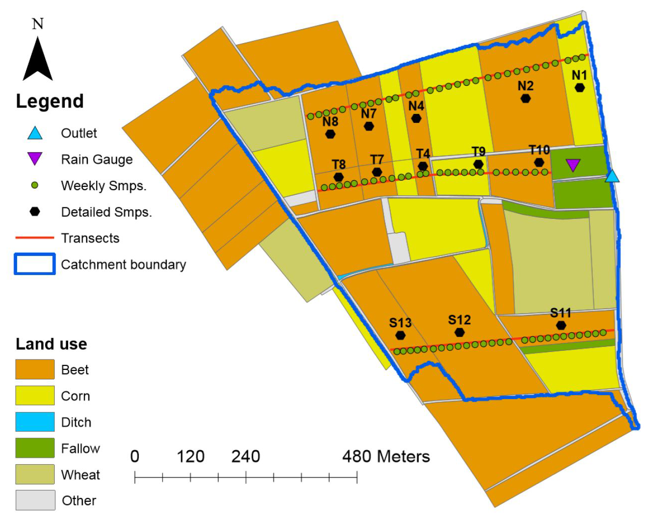
Figure 1 The Alteckendorf headwater catchment (Bas-Rhin, France) showing the experimental setup, including three transects, i.e. north, valley, and south (weighted samples collected at green dots along the red lines), and plot sampling (black dots). Land use for 2016 is also displayed. The “other” category includes roads, grass strips, and orchards.

Daily temperature and potential evapotranspiration were obtained from the MétéoFrance station in Waltenheim-sur-Zorn, located 7 km southwest of the study site. Daily rainfall was measured using a tipping bucket rain gauge (Précis Mécanique^®, Fig. 1). Detailed climate and hydrological data are provided in Table S1 in the Supplement. The catchment is predominantly arable land, with corn (18 %), sugar beet (70 %), and wheat (3 %) as the main crops in 2016. A subsurface tile drainage system of unknown spatial extent is present at a depth of 0.8 m. Water is collected via ditches and discharged through a 50 cm diameter pipe at the catchment outlet (Fig. 1). Soils are classified as Haplic Cambisol (Calcaric, Siltic) and Eutric Cambisol (Siltic) on hillsides (north and south) and Eutric Cambisol (Colluvic, Siltic) in the central valley. Soil analysis from 48 topsoil samples (0–20 cm) and six 2 m depth profiles showed low spatial variability across the catchment (Lefrancq et al., 2018). The texture is predominantly silt (61.0 % ± 4.5 %), followed by clay (30.8 % ± 3.9 %) and sand (8.5 % ± 4.2 %). The soil also contains calcium carbonate (CaCO₃: 1.1 % ± 1.6 %), organic matter (2.2 % ± 0.3 %), and total soluble phosphorus (0.11 ± 0.04 g kg⁻¹) and has cation exchange capacity (CEC: 15.5 ± 1.3 cmol kg⁻¹). Soil pH averaged 6.7 ± 0.8 (n=30). A compacted plough layer was observed between 20 and 30 cm in depth. In 2016, S-metolachlor was applied to corn and sugar beet plots in three applications: 20–25 March, 13–14 April, and 25–31 May. These plots covered 88 % of the catchment area. Application dates, doses, and formulation were obtained for each plot from farmer surveys, providing spatially distributed data for modelling. In total, 20.2, 5.9, and 14.0 kg of S-metolachlor were applied to the north, valley, and south transects, respectively (Table S2 in the Supplement).

2.2 Soil and water sampling and outlet discharge measurements

Samples from the topsoil (0–1 cm) were collected from individual plots and upstream–downstream transects across the catchment (Figs. 1 and S1 in the Supplement; Alvarez-Zaldivar et al., 2018). A total of 13 marked plots were sampled before S-metolachlor application and on days 1, 50, and 100 after application. In addition, weekly weighted composite samples were taken along the north, valley, and south transects (green dots in Fig. 1) from 19 March (day 0) to 12 July (day 115). All soil samples were analysed for S-metolachlor concentration and carbon isotope composition (δ¹³C) using CSIA. The volumetric topsoil water content (${\mathrm{m}}_{\text{water}}^{\mathrm{3}}{\mathrm{m}}_{\text{soil}}^{-\mathrm{3}}$) was calculated from gravimetric measurements after drying samples at 110 °C following NF ISO 1146 (Lefrancq et al., 2018). This procedure was applied to field samples collected on days 1, 50, and 100 after application, as well as the weekly mixed samples from the three transects. It incorporated seasonal variations in topsoil bulk density, as modelled by PiBEACH and detailed in Sect. S7.2 in the Supplement.

Runoff discharge at the catchment outlet was measured using a Doppler flowmeter (2150 Isco) with 3 % accuracy and a 2 min resolution. Continuous, refrigerated, and flow-proportional sampling was carried out using an Isco Avalanche autosampler equipped with 12 330 mL bottles. Samples were collected based on fixed weekly discharge volumes from 50 to 150 m³ in order to capture progressive increases in baseflow discharge from April to June 2016 (Alvarez-Zaldivar et al., 2018). To obtain sufficient S-metolachlor for quantification and CSIA, weekly composite samples were prepared by pooling bottles according to the hydrograph phase (baseflow, rising limb, and falling limb), yielding one to four samples per week with volumes of ≥990 mL (Alvarez-Zaldivar et al., 2018). Piezometric monitoring of the shallow aquifer was not possible due to the absence of observation wells at the study site.

2.3 S-metolachlor quantification and δ¹³C analysis

To separate the dissolved and particulate phases of S-metolachlor, river water samples were filtered through 0.7 µm glass fibre filters. Extraction of S-metolachlor from soil and water samples was performed using an AutoTrace 280 solid-phase extraction (SPE) system (Dionex) with SolEx C18 cartridges (Dionex^®), as previously described (Alvarez-Zaldivar et al., 2018; Gilevska et al., 2022b). The quantification was carried out using chromatography–mass spectrometry (GC-MS, ISQ™, Thermo Fisher 173 Scientific). Quantification limits were 0.01 µg L⁻¹ for water and 0.001 µg g⁻¹ (dry weight) for soil and suspended matter, with a total analytical uncertainty of 8 % and 16 %, respectively. Carbon isotope ratios (δ¹³C) of S-metolachlor in soil and water were analysed using a GC-C-IRMS (gas chromatography–combustion–isotope ratio mass spectrometry), comprising a TRACE™ Ultra gas chromatograph (ThermoFisher Scientific) coupled to a Delta V plus isotope ratio mass spectrometer via a GC IsoLink/Conflow IV interface (Alvarez-Zaldivar et al., 2018; Gilevska et al., 2022b; see also Sect. S5 in the Supplement). The reproducibility of triplicate δ¹³C measurements was ≤0.2 ‰ (1σ). A minimum peak amplitude of 300 mV, corresponding to approximately 10 ng of carbon injected into the column, was required for accurate isotope analysis.

2.4 PiBEACH model description

PiBEACH development. The Pesticide isotope BEACH model (PiBEACH) was developed in Python based on the conceptual Bridge Event And Continuous Hydrological (BEACH) model (Sheikh et al., 2009). BEACH was chosen for its demonstrated ability to simulate daily topsoil moisture and catchment discharge with high accuracy (Nash–Sutcliffe efficiency of 0.79) in a 42 ha catchment (Sheikh et al., 2009) with loess soils and crops similar to those observed in the study catchment. BEACH is a grid-based model that simulates spatially distributed soil water content and catchment outlet discharge by accounting for key hydrological processes, including evaporation, plant transpiration, percolation, deep percolation, lateral flow, and runoff (Sheikh et al., 2009). Similar to BEACH, the PiBEACH model employs square cells (x,y) with variable depths (z) corresponding to the soil layers considered (Fig. 2) in order to represent water and pesticide movement within the catchment, as detailed below. At the cell scale, daily vertical water fluxes are computed across soil layers, followed by lateral fluxes upstream to downstream. Surface flow direction is derived from the digital elevation model using flow-accumulation functions without employing a numerical scheme (Sheikh et al., 2009).

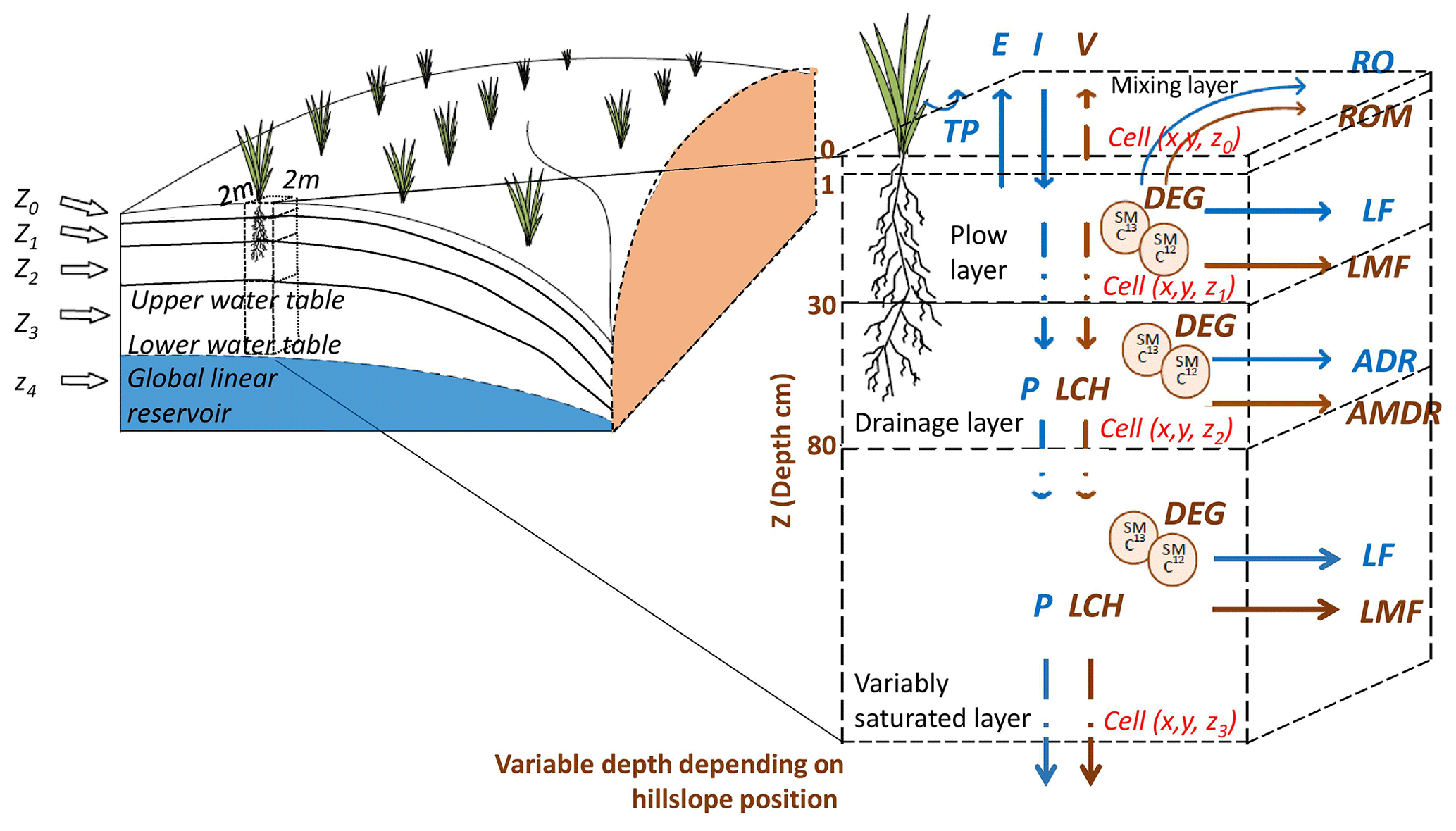
Figure 2 Conceptual representation of the five-layer (z₀ to z₄) spatially distributed hydrological and reactive transport model PiBEACH, employing a 2 m×2 m raster resolution and variable depths depending on soil layers from z₀ to z₃. Hydrological processes include evaporation (E), transpiration (TP), percolation (P), volatilisation (V), runoff (RO), lateral flow (LF), and artificial drainage (ADR). Pesticide mass transfer processes include volatilisation (V), runoff mass (ROM), lateral mass flow (LMF), leaching (LCH), mass transfer via artificial drainage (AMDR), and degradation (DEG) with isotope fractionation (SM ¹³C and SM ¹²C).

The model is driven by daily meteorological records (rainfall, air temperature, and potential evaporation), soil physical properties (saturated hydraulic conductivity, bulk density, and porosity for both the plough layer and a deeper soil layer), and crop-specific agronomic parameters. PiBEACH extends BEACH by incorporating experimental knowledge of hydrological and pesticide transport processes observed in the Alteckendorf catchment (Lefrancq et al., 2017, 2018; Lutz et al., 2017; Alvarez-Zaldivar et al., 2018; Lange et al., 2018). It translates the perceptual model developed by field researchers into a conceptual framework, following the approach of Ammann et al. (2020).

Key modifications in PiBEACH include (i) a topsoil mixing layer, assuming that pesticide transport is controlled by a mixing layer from 0.25 to 2 cm below the soil surface, in which rainfall, soil solution, and runoff are assumed to mix instantaneously (McGrath et al., 2008), and by deeper soil layers to capture groundwater contributions to discharge; (ii) daily simulation of topsoil temperature (Neitsch et al., 2011); (iii) daily dynamic topsoil hydraulic properties that reflect crop-specific agronomic practices (Lefrancq et al., 2018); (iv) first-order pesticide degradation and linear sorption/desorption; and (v) pesticide carbon stable-isotopic fractionation and transport of bulk heavy and light carbon in the pesticide molecule (e.g. ¹³C and ¹²C) (Lutz et al., 2017; Alvarez-Zaldivar et al., 2018). PiBEACH requires spatially explicit inputs of pesticide application dates and quantities for each plot.

Comparison of PiBEACH with physically based models. The finite difference or finite volume method is typically used to simulate agricultural catchment hydrology in 3D physically based models, e.g. Hydrogeosphere (De Schepper et al., 2015) or CATHY (Gatel et al., 2020). However, modelling pesticide reactive transport, including pesticide sorption–desorption and degradation on the catchment scale, remains challenging. This challenge arises because numerical dispersion can affect the mass balance at the catchment scale (Gatel et al., 2020) to an extent comparable to the pesticide export coefficient, defined as the ratio of the mass transported at the outlet to the total mass applied within the catchment, which typically ranges from 0.1 ‰ to 1 % of the applied pesticide load (Lefrancq et al., 2018).

The numerical dispersion issues can be mitigated, although this leads to longer computation times in both 2D (Lutz et al., 2013) and 3D (Gatel et al., 2020) models. PiBEACH simulates water and pesticide fluxes on a daily time step, tracking flow from upstream to downstream along branches of the drainage network using flow-accumulation grid-based functions (Sheikh et al., 2009). While it avoids numerical issues by not employing differential equations and associated numerical schemes, this approach also limits its ability to predict fast-flow dynamics, i.e. runoff genesis and preferential water flow. The drainage network can be extracted from a lidar digital elevation model (Lefrancq et al., 2017). The vertical mass balance is computed using the sum of discharge and pesticide masses of the upstream grid cells as lateral inputs for the downstream grid cells (Sect. S6 in the Supplement and Eq. 2). The daily resolution of PiBEACH reduced the computation time by 1 to 2 orders of magnitude compared to 2D or 3D models for catchments of a similar size (Gatel et al., 2020). The limitations associated with this conceptual approach are discussed in the next section.

PiBEACH description and submodel components. To account for landscape features affecting pesticide off-site transport, such as grass strips or roads, the Alteckendorf catchment was modelled using a 2 m×2 m raster resolution. The vertical soil profile was divided into five successive layers from the topsoil to the groundwater (Fig. 2): (i) a surface mixing layer (z₀: 0–1 cm) (McGrath et al., 2008); (ii) a plough layer observed in the field (z₁: 1–30 cm); (iii) a drainage layer controlled by tile drains, as observed in the Alteckendorf catchment (z₂: 30–80 cm); (iv) a variably saturated layer (z₃); and (v) a permanently saturated groundwater layer (z₄). The combined groundwater depths (z₃+z₄) varied spatially and seasonally across the catchment, with a maximum observed depth of 23.2 m, consistent with recharge dynamics in the monitored hillslopes (Molénat et al., 2005). The partitioning between z₃ and z₄ was defined as a calibration parameter z_f, such that if $z_{\mathrm{3}}+z_{\mathrm{4}}=\mathrm{23.2}$ m, $z_{\mathrm{3}}=\mathrm{23.2}\times z_f$ and $z_{\mathrm{4}}=\mathrm{23.2}\times (\mathrm{1}-z_f)$ (Table S3 in the Supplement).

The hydrological balance follows the formulation of Sheikh et al. (2009), with process-specific implementations detailed in Sect. S6. For each grid cell i of each soil layer zj, the daily change in volumetric soil water content (θ, m³ m⁻³) is calculated using

$$\begin{array}{}\text{(1)}& \begin{array}{rl}\mathrm{\Delta }{\mathit{\theta }}_i=& R_{i,zj}-{\text{RO}}_{i,zj}+\mathrm{\Delta }{\text{LF}}_{i,zj}-{\text{Ea}}_{i,zj}\\ & -{\text{Ta}}_{i-zj}-P_{i,zj},\end{array}\end{array}$$

where daily rainfall (R), runoff (RO) (calculated for z0), net cell lateral inflow–outflow (ΔLF), actual evaporation (Ea), actual transpiration (Ta), and percolation (P) were expressed in mm H₂O d⁻¹. Four layers, z₀ to z₃, are present in Eq. (1). Evaporation (Ea) affects layers z₀ to z₃, while transpiration (Ta) depends on plant root depth following crop-specific development stages (see Sect. S6.5 and S6.6 in the Supplement). Lateral flow (ΔLF) and percolation (P) are calculated from upstream to downstream cells for layers z₀ to z₃ (Manfreda et al., 2005). Percolation across the saturated layer z₄ is routed to the outlet as a global linear reservoir (Manfreda et al., 2005).

The agronomic submodel of PiBEACH (Lefrancq et al., 2017) (see Sect. S7 in the Supplement) simulates seasonal variation in topsoil hydraulic properties, improving the hydrological balance of the headwater catchment (Lefrancq et al., 2017).

The pesticide dissipation submodel of PiBEACH represents the key processes governing pesticide reactive transport at the catchment scale (Fig. 2). The pesticide mass (M, g) balance for each cell i and each layer is expressed as

$$\begin{array}{}\text{(2)}& {\displaystyle \frac{\mathrm{d}{M}_i}{\mathrm{d}t}}=A_i-{\text{ROM}}_i+\mathrm{\Delta }{\text{LMF}}_i-V_i-{\text{LCH}}_i-{\text{DEG}}_i,\end{array}$$

where M is the pesticide mass (g), A is the applied mass (g d⁻¹), ROM is mass lost via runoff (z0 only), ΔLMF is lateral mass flow (z0–z3), V is volatilisation (z0), LCH is leaching (z0–z3), and DEG is degradation (z0–z4).

Pesticide partitioning into dissolved, sorbed, and gaseous phases follows Leistra et al. (2001) (see Sect. S8 in the Supplement). Partitioning into the dissolved and adsorbed phases was determined by linear sorption, considering the organic carbon–water partition coefficient K_OC (mL g⁻¹) normalised by the fraction of organic carbon f_OC (kg kg⁻¹) in soil, where the pesticide dissociation coefficient (K_d, mL g⁻¹) is given by $K_{\mathrm{d}}=K_{\text{OC}}\times f_{\text{OC}}$. Partitioning into the gas phase was obtained from the dimensionless Henry constant, $K_{\mathrm{H}}^{\text{cc}}=\mathrm{9.55}\times {\mathrm{10}}^{-\mathrm{5}}$, for S-metolachlor (Feigenbrugel et al., 2004). General pesticide mass flux J (µg d⁻¹) for each model cell is computed as

$$\begin{array}{}\text{(3)}& J=q_{x,y}\times C_{\text{aq}},\end{array}$$

where q_x,y is the water flux (mm d⁻¹) in the lateral (x,y) direction, and C_aq is the dissolved S-metolachlor concentration in the aqueous phase (µg mm⁻¹). In the topsoil layer (z₀), runoff and volatilisation are included:

$$\begin{array}{}\text{(4)}& J_{zo}=q_{x,y}+c_{\text{aq}}\left(\text{RO}{e}^{-{\mathit{\beta }}_{\text{RO}}{D}_{zo}}+{\displaystyle \frac{\mathrm{1}}{r_{\mathrm{a}}+r_{\mathrm{s}}}}\right),\end{array}$$

where RO is runoff (mm), β_RO is a calibration constant ($\mathrm{1}\ge {\mathit{\beta }}_{\text{RO}}\ge \mathrm{0}$), and D_z0 (mm) is the mixing layer depth (Ahuja and Lehman, 1983). Volatilisation was limited to the first 5 d after application (Gish et al., 2011; Prueger et al., 2005) and follows Leistra et al. (2001), with fluxes across topsoil controlled by air transport resistance, r_a (d m⁻¹), and diffusion resistance, r_s (d m⁻¹) (Leistra et al., 2001, and Sect. S8.2 in the Supplement).

Biodegradation occurs only in bioavailable fractions of adsorbed (ads) and aqueous (aq) phases (Thullner et al., 2013). A similar stable-isotope fractionation associated with degradation was then considered for the bioavailable fractions, including the adsorbed (Eq. 5, second term) and the aqueous (Eq. 6) phases. The bioavailable fraction was controlled kinetically by the ageing rate k_age (d⁻¹) of the adsorbed fraction (Schwarzenbach et al., 2003). Due to the physicochemical properties of S-metolachlor, abiotic degradation processes (such as photolysis) and their associated isotope fractionation were excluded from the model. While non-destructive processes like dispersion and sorption may induce isotope fractionation under conditions of strong sorption behaviour, of transient diffusion, or of repeated sorption–desorption cycles (Eckert et al., 2013; van Breukelen and Prommer, 2008; van Breukelen and Rolle, 2012; Kopinke et al., 2017), these effects were considered negligible. Given the rapid biodegradation of S-metolachlor in soil and the limited impact of sorption-induced fractionation in surface agro-ecosystems, only biodegradation-induced fractionation was included in the model. Since non-significant alteration of the isotope composition of pollutants was expected during sorption and ageing (Schmidt et al., 2004; Droz et al., 2021), the ratios of light to heavy isotopologues did not significantly vary during the sorption and ageing processes (Eq. 5, first term). In our case, since isotope fractionation associated with the sorption and ageing processes is expected to be negligible, the observed isotope fractionation can be attributed primarily to biodegradation. This justifies the exclusion of non-destructive processes from the isotope mass balance and supports the use of the model to distinguish between destructive, i.e. biodegradation, and non-destructive processes, thereby enabling a quantitative evaluation of the contribution of biodegradation to pesticide dissipation. Altogether, by representing pesticide mass (M) as separate light (l) and heavy (h) isotopologues, the change in aqueous and adsorbed phases is expressed as

$$\begin{array}{}\text{(5)}& {\displaystyle \frac{\mathrm{d}{M}_{\text{ads}}}{\mathrm{d}t}}=-k_{\text{age}}(M_{\text{ads}}^{\mathrm{l}}+M_{\text{ads}}^{\mathrm{h}})-k_{\text{deg}}(M_{\text{ads}}^{\mathrm{l}}+\mathit{\alpha }{M}_{\text{ads}}^{\mathrm{h}})\text{(6)}& {\displaystyle \frac{\mathrm{d}{M}_{\text{aq}}}{\mathrm{d}t}}=-k_{\text{deg}}(M_{\text{aq}}^{\mathrm{l}}+\mathit{\alpha }{M}_{\text{aq}}^{\mathrm{h}}),\end{array}$$

where $k_{\text{deg}}=\ln \left(\mathrm{2}\right)/{\text{DT}}_{\mathrm{50}}$, and DT₅₀ (d) is the observed degradation half-life in soil. Stable-isotope fractionation associated with S-metolachlor degradation in soil was considered through the carbon fractionation factor (α_C), expressed as ${\mathit{\alpha }}_{\mathrm{C}}={\mathit{\epsilon }}_{\mathrm{C}}/\mathrm{1000}+\mathrm{1}$, where ε_C (‰) was the carbon stable-isotope fractionation value of the targeted pesticide retrieved from a degradation reference experiment. The degradation rates for S-metolachlor freshly sorbed in the organic fraction of soil was assumed to be equal to the degradation rates in the dissolved phase (Wu et al., 2011; Long et al., 2014). The reduction in bioavailability of the aged fraction of S-metolachlor as a function of the increasing fraction of irreversibly sorbed S-metolachlor over time (Sander et al., 2006; Arias-Estevez et al., 2008; Torabi et al., 2020) was taken into account with the rate k_irs (d⁻¹) of irreversible sorption for the aged S-metolachlor mass (M_age, g):

$$\begin{array}{}\text{(7)}& {\displaystyle \frac{\mathrm{d}{M}_{\text{age}}}{\mathrm{d}t}}=-k_{\text{irs}}(M_{\text{age}}^{\mathrm{l}}+M_{\text{age}}^{\mathrm{h}}).\end{array}$$

The decrease in M_age due to abiotic degradation (Xu et al., 2018) was not included since it was unlikely to be significant under abiotic conditions in the aerobic soil studied (Torabi et al., 2020), even after 200 d of incubation (Alvarez-Zaldivar et al., 2018).

Pesticide degradation rates generally decline with soil depth due to reduced microbial activity (Cruz et al., 2008; Lutz et al., 2017) and increased sorption (Arias-Estevez et al., 2008) in deeper layers. However, the absence of concentration and CSIA data for S-metolachlor in subsoil prevented direct quantification of depth-dependent degradation. Following the approach used in advanced pesticide fate models such as MACRO (Garratt et al., 2003), the degradation rate (k_deg) in PiBEACH was modelled as a function of soil hydro-climatic conditions, such as soil temperature and water content. A dynamic degradation rate (k_dynamic, d⁻¹) was calculated daily as a function of soil temperature (F_T; unitless) and of water content (F_θ; unitless):

$$\begin{array}{}\text{(8)}& k_{\text{dynamic}}=k_{\text{ref}}\times F_T\times F_{\mathit{\theta }},\end{array}$$

where k_ref (d⁻¹) was the degradation rate constant from the degradation half-life (d) at reference conditions ($k_{\text{ref}}=\ln \left(\mathrm{2}\right)/{\text{DT}}_{\mathrm{50},\text{ref}}$). A dynamic half-life, DT_50,dynamic, was derived to be compared to DT_50,ref (${\text{DT}}_{\mathrm{50},\text{dynamic}}=\ln \left(\mathrm{2}\right)/k_{\text{dynamic}}$).

For soil temperature dependence, the modified Arrhenius equation for low temperatures was considered (Boesten and Vanderlinden, 1991; Larsbo and Jarvis, 2003):

$$\begin{array}{}\text{(9)}& F_T=\left\{\begin{array}{ll}\mathrm{0},& \text{if }{T}_{\mathrm{C}}\le \mathrm{0}\\ \frac{T_{\mathrm{K},\text{obs}}-\mathrm{273.15}}{\mathrm{5}}& \\ \times \exp \left(\frac{E_{\mathrm{a}}}{R}\left(\frac{\mathrm{1}}{T_{\mathrm{K},\text{ref}}}-\frac{\mathrm{1}}{T_{\mathrm{K},\text{obs}}}\right)\right),& \text{if }\mathrm{0}<T_{\mathrm{C}}\le \mathrm{5}\\ \exp \left(\frac{E_{\mathrm{a}}}{R}\left(\frac{\mathrm{1}}{T_{\mathrm{K},\text{ref}}-\frac{\mathrm{1}}{T_{\mathrm{K},\text{Obs}}}}\right)\right),& \text{if }{T}_{\mathrm{C}}>\mathrm{5}\end{array}\right.,\end{array}$$

where T_K and T_C were soil temperatures in Kelvin and Celsius, respectively, and T_K,ref was the reference temperature at 293.15 K. E_a was the S-metolachlor activation energy (23.91×10³ J mol⁻¹) (Jaikaew et al., 2017), and R was the gas constant (8.314 $\mathrm{J}{\mathrm{mol}}^{-\mathrm{1}}{\mathrm{K}}^{-\mathrm{1}}$). This modified Arrhenius equation was validated against the DT₅₀ values derived from microcosm degradation experiments with S-metolachlor conducted at 20 and 30 °C (Sect. S9, Fig. S4 in the Supplement).

The influence of water content followed Walker (1974) and Larsbo and Jarvis (2003):

$$\begin{array}{}\text{(10)}& F_{\mathit{\theta }}=min\left(\mathrm{1.0},{\left({\displaystyle \frac{{\mathit{\theta }}_t}{{\mathit{\theta }}_{\text{ref}}}}\right)}^{{\mathit{\beta }}_{\mathit{\theta }}}\right),\end{array}$$

where β_θ was a calibration constant and θ_ref the reference water content, which was set to 0.2 m³ m⁻³. Note that F_θ was slightly modified from Walker (1974), as microcosm experiments for S-metolachlor did not show an increase in degradation rates with increases in moisture content (Fig. S4).

Calibrating the PiBEACH parameters, as detailed in Sect. 2.6, was challenging and warranted the collection of an extensive dataset across the catchment throughout the growing season. This unique dataset incorporated isotopic signatures and comprised 103 topsoil samples analysed for S-metolachlor concentration and δ¹³C, 115 daily discharge measurements, and 51 river water samples at the outlet with corresponding S-metolachlor concentrations.

2.5 Model limitations

Although PiBEACH was primarily developed to simulate pesticides dissipation in topsoil, four aspects of its design may limit its application when predicting pesticide dynamics at the outlet of the headwater catchment. First, PiBEACH operates on a daily time step and is not suitable for capturing rapid-flow dynamics, such as runoff generation and event-scale hydrological dynamics (Sheikh et al., 2009). Consequently, S-metolachlor concentrations and corresponding δ¹³C values measured at the catchment outlet were not included in the model calibration objective function. This limitation could be addressed by coupling PiBEACH with a distributed event-based model, such as the Limburg Soil Erosion Model (OpenLISEM) (Baartman et al., 2012), which recently integrated a pesticide module (OLP) (Commelin et al., 2024). Second, PiBEACH uses a conceptual linear reservoir to represent shallow-aquifer dynamics and does not explicitly simulate the effects of transit time distribution on the pesticide release from groundwater into surface water (Hrachowitz et al., 2016). While incorporating transit time distributions into a lumped reactive transport model has shown promise (Lutz et al., 2017), applying such an approach to a distributed model remains challenging, as demonstrated for nitrate (Kaandorp et al., 2021).

In addition, pesticide leaching across soil layers was considered without distinguishing between matrix and preferential flows. Macropores can also play a significant role in pesticide breakthrough in the vadose zone (Urbina et al., 2020). However, the integration of macropores at the catchment scale necessitates advanced in situ measurements (Weiler, 2017) and a combination of geostatistical methods; pedotransfer functions; or meta-models, i.e. simplified statistical models built with 1D soil reactive transport models such as MACRO (Lindahl et al., 2008).

PiBEACH integrates the main catchment compartments, including soil layers, vegetation and crops, and major processes controlling pesticide fate. However, plant uptake of S-metolachlor was not included, as it is likely negligible (Lefrancq et al., 2018). Additionally, pesticide wash-off from plants was not considered in PiBEACH, as S-metolachlor is a pre-emergent herbicide applied on bare soil.

Considering degradation in reactive transport models as a lumped process with only one half-life parameter is a strong simplification, which may alter the predictability of degradation in models. However, this limitation is shared among existing pesticide transport models (Leistra et al., 2001; Lindahl et al., 2008; Lutz et al., 2017; Gatel et al., 2020). The implementation of the soil temperature and moisture dependence of pesticide degradation, as proposed in this study, may strengthen the description of degradation within the catchment and across the hydrological or growing season (Gassmann, 2021). Nonetheless, soil temperature and moisture are also forcing variables of the soil microbial activity, and thus of biodegradation, which remains extremely difficult to characterise and conceptualise with respect to pesticide transformation (Imfeld and Vuilleumier, 2012; Bongiorno, 2020; Höhener et al., 2022) for implementation in reactive models at the catchment scale.

2.6 Model uncertainty assessment

The GLUE and formal Bayesian methods are commonly used methods to quantify the uncertainty in hydrological models and to provide distributions of parameters and water discharge. Bayesian methods are more convenient to calculate the uncertainty interval of one-step-ahead forecasting with a formal- or exact-likelihood function (Jin et al., 2010). In contrast, the GLUE method integrates a true-calibration process in which both inputs and model structural errors contribute to uncertainties in the model outputs (Beven et al., 2007). The GLUE method was thus adopted in our study to calibrate PiBEACH and retrieve output uncertainties. Rather than seeking an optimal model solution, the GLUE approach recognises that more than one model structure or parameter set may lead to acceptable model results, i.e. equifinality (Beven and Binley, 1992). The GLUE method involved sampling PiBEACH parameter values, an objective function incorporating the observed dataset (i.e. topsoil S-metolachlor concentration only, then combined with S-metolachlor δ¹³C), a threshold of this objective function to select behavioural parameter sets, and the calculation of posterior probability distributions for parameters and uncertainties associated with the outputs of PiBEACH.

For the method sampling the parameters, PiBEACH required the calibration of 43 parameters (Table S3). The range, i.e. min–max values, of these parameters was defined based on either the literature or field data collected in 2012 and 2016 (Lefrancq et al., 2017, 2018; Alvarez-Zaldivar et al., 2018). These parameters were assumed to be a priori uniformly distributed within these min and max values (Table S3). To reduce the number of runs required by the GLUE method, three steps were successively applied. First, a pre-sensitivity global analysis based on the Morris method (Morris, 1991; Herman and Usher, 2017; Campolongo et al., 2007) was conducted using the SALib Python library for sensitivity analysis (Sect. S10 in the Supplement) to select the most sensitive parameters. Although the Morris method yields a qualitative indication of relative parameter importance, it is efficient compared to other sensitivity approaches (Gan et al., 2014) that screen for sensitive parameters (Herman et al., 2013). The mean and standard deviation of the elementary effects (EEs) for each parameter were calculated as required by the Morris method. The mean represents the overall effect of a parameter on the model output, while the standard deviation captures the potential for interactions or nonlinear effects. Parameters with a mean EE of zero or near-zero, indicating negligible impact, were excluded, resulting in the removal of 21 parameters. The sensitivity analysis was conducted for the following outputs: S-metolachlor concentrations at the outlet, concentrations in composite topsoil transects (north, valley, and south), discharge at the outlet, and isotope signatures in the river at the outlet and within the topsoil composite transects. The EE statistics for the 25 parameters retained are shown in Figs. S5 and S6 in the Supplement for each output variable.

The Morris method allowed us to reduce the PiBEACH parameter number from 43 to 25 (Table S3). Second, Latin-hypercube sampling (Herman and Usher, 2017) was used to reduce the numbers of runs (n=2500) to cover the parameter space for the 25 parameters. To further reduce the computation time, the GLUE assessment focused on the growing period (19 March to 12 July 2016), when pesticide degradation and exports are most significant. The initial hydrological state was estimated from a spinup period of 1 full hydrological year (1 October 2015–30 September 2016) and from hydrological parameters calibrated against discharge observed at the catchment outlet (19 March and 12 July 2016) using particle swarm optimisation (Bratton and Kennedy, 2007).

For the second step of the GLUE method, the Kling–Gupta efficiency (KGE) (Gupta et al., 2009) metric was adopted as the objective function to maximise during calibration. Goodness of fit between simulations and observations is given relative to a maximum efficiency of 1 and is given by

$$\begin{array}{}\text{(11)}& \text{KGE}=\mathrm{1}-\sqrt{(r-\mathrm{1}{)}^{\mathrm{2}}+({\mathit{\alpha }}_{\text{KGE}}-\mathrm{1}{)}^{\mathrm{2}}+({\mathit{\beta }}_{\text{KGE}}-\mathrm{1}{)}^{\mathrm{2}}},\end{array}$$

where r is the linear correlation coefficient between simulated and observed values; ${\mathit{\alpha }}_{\text{KGE}}={\mathit{\sigma }}_i/{\mathit{\sigma }}_{\mathrm{0}}$; and ${\mathit{\beta }}_{\text{KGE}}={\mathit{\mu }}_i/{\mathit{\mu }}_{\mathrm{0}}$, where σ and μ denote the standard deviation and mean of simulated and observed values, respectively.

The KGE metric was selected to provide equal weight across correlation, bias, and variability measures. The Kling–Gupta efficiency (KGE) provides a more balanced assessment of model performance than traditional metrics such as the mean squared error (MSE) or Nash–Sutcliffe efficiency (NSE), which often favour parameter sets that underestimate output variability (Gupta et al., 2009). Three KGE metrics were calculated: (i) KGE_SM with weekly topsoil S-metolachlor concentration, (ii) KGE_δ with weekly topsoil δ¹³C, and (iii) KGE_Q with daily discharge at the outlet. The KGE metrics were successively built to assess the benefit of CSIA by incorporating topsoil S-metolachlor concentrations only or in combination with topsoil S-metolachlor δ¹³C observations. For the latter, the KGE metric incorporates topsoil S-metolachlor concentration and δ¹³C from (i) individual plot observations (13 black dots, Fig. 1), (ii) aggregated plot observations along three transects across the catchment (north, valley, and south transects, Fig. 1), and (iii) transect composite soil (green dots, Fig. 1). These three approaches to aggregating topsoil data were developed to determine the minimum sampling effort for S-metolachlor concentration and for δ¹³C required to minimise uncertainties in PiBEACH model outputs.

According to the classification proposed by Kling et al. (2012) and subsequently adopted by Towner et al. (2019), the goodness of fit between simulated and observed variables is categorised as “very poor” for KGE≤0, “poor” for KGE≤0.5, “intermediate” for KGE≤0.75, and “good” for KGE>0.75; the threshold to retain acceptable model results runs (out of 2500 simulation runs) for topsoil S-metolachlor degradation and transport was set to KGE_SM>0.5 and KGE_Q>0.5. An additional and more stringent criterion (KGE_δ>0.8) was applied to weekly topsoil δ¹³C data to maximise its value as an indicator of degradation processes. These thresholds were ultimately selected as a compromise, enabling the retention of simulations with at least intermediate accuracy, while preserving a sufficient number of parameter sets to support the derivation of outputs with robust confidence intervals.

In the final step of the GLUE procedure, the distributions of the 25 most sensitive parameters were extracted from the subset of acceptable parameter sets, i.e. KGE_SM>0.5, KGE_Q>0.5, and KGE_δ>0.8. PiBEACH outputs were then expressed as the mean considering the 95 % confidence intervals based on these parameter sets, excluding the lower 2.5 % and the upper 2.5 % of acceptable simulations.

2.7 Metrics of pesticide persistence and transport risks

Six metrics were derived from PiBEACH outputs to assess S-metolachlor persistence and transport risk at the catchment scale. Expressed as percentages of the applied mass, these metrics included (1) S-metolachlor degradation, (2) the remaining bioavailable mass (BAM) of S-metolachlor in the topsoil (i.e. dissolved and reversibly sorbed S-metolachlor), (3) S-metolachlor export to the catchment outlet via runoff and drainage, (4) off-site transport of S-metolachlor through leaching, (5) the remaining mass of irreversibly sorbed S-metolachlor (i.e. aged S-metolachlor), and (6) S-metolachlor volatilisation from the first application on 19 March (day 0) to 12 July 2016 (day 115). The first three metrics were also derived from field observations to evaluate the predictive accuracy of PiBEACH. Observed BAM in the topsoil was estimated through spatial extrapolation of weekly soil samples. The observed S-metolachlor degradation was estimated using the mean δ¹³C derived from the same spatial extrapolation combined with the isotopic fractionation factor (ε) obtained from microcosm lab-scale experiments using soil from Alteckendorf. Export to the outlet was calculated by integrating continuous discharge measurements with sub-weekly river S-metolachlor concentrations. The remaining three metrics, leaching, volatilisation, and ageing, could not be estimated from field data due to limitations of the catchment-scale sampling campaign and were therefore not computed from observations.

3 Results and discussion

3.1 Topsoil hydro-climatic dynamics and effect on S-metolachlor degradation rates

Simulated topsoil (z₀) water contents showed substantial variability, consistent with weekly field measurements (Fig. 3a) and previous application of the BEACH model in catchments with similar soils, crops, and conditions (Sheikh et al., 2009). Simulated discharges at the catchment outlet showed reasonable agreement with observations (Fig. 3b), with a maximum KGE_Q of 0.75, demonstrating the model's ability to capture prevailing hydrological dynamics. However, PiBEACH slightly overestimated runoff generation, a known limitation related to the underlying assumptions of the SCS-CN (soil conservation service – curve number) method (Sect. S6.2 in the Supplement) and to the use of a daily time step, which does not resolve sub-daily rainfall intensity. Hydro-climatic variability drove changes in the simulated degradation rates (k_dynamic) and associated half-lives (DT_50,dynamic) of S-metolachlor over time (Fig. 3c). Low S-metolachlor degradation rates during the first 10 d (DT₅₀=46 ± 17 d) coincided with a cold (7.1 ± 1.7 °C) and dry period (7.4 mm of rainfall) (Fig. 3a). In contrast, increasing degradation rates (DT₅₀=22 ± 2 d) between 50 and 120 d following the first application of S-metolachlor were associated with warmer conditions (16.9 ± 3.6 °C). Between March and July, topsoil temperatures increased, creating a stronger vertical temperature gradient and leading to reduced degradation activity at greater depths. In July, for instance, DT₅₀ values were estimated at 25 d in the topsoil (Fig. 3c) and at 34 d at 2 m in depth (data not shown), consistent with predictions from the lumped model developed by Lutz et al. (2017) for this catchment. Simulated S-metolachlor concentrations (Fig. 3d) and carbon isotope ratios (Fig. 3e) in topsoil aligned with weekly field observations, confirming the model's ability to reproduce both concentration dynamics and isotopic trends.

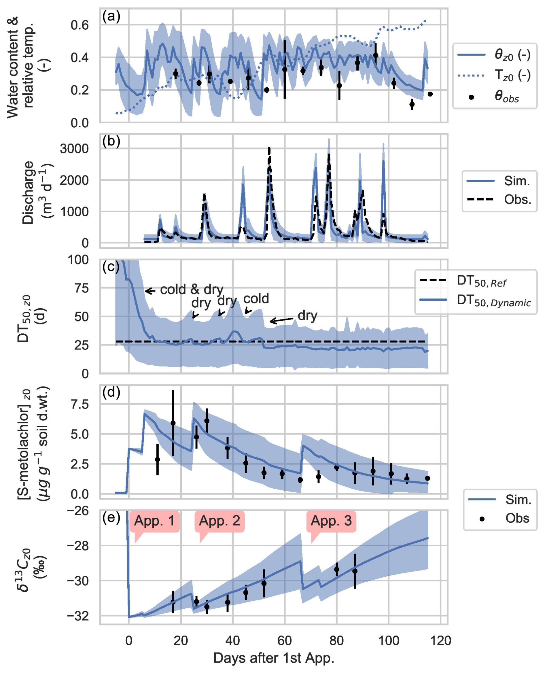
Figure 3 Predicted water content (m³ m⁻³) and relative topsoil temperatures ($T_{z\mathrm{0}}/T_{\text{air,\hspace{0.17em}max}}$, with T_air, max=27 °C) in the topsoil layer (z₀: 0–1 cm) from 14 March (day −5, before first application) and 12 July (day 115). The shaded area indicates the 95 % confidence intervals (CIs). Weekly observed water content (θ_obs) in topsoil is also shown (a), with error bars reflecting uncertainties in soil bulk density (used for gravimetric-to-volumetric conversion) and the standard error in gravimetric water content measurements. (b) Simulated and observed daily outlet discharge at the catchment scale, with the shaded area representing 95 % CIs of the model ensemble. (c) Simulated mean dynamic degradation half-life (DT_50,dynamic) of S-metolachlor in the topsoil (z₀); the 95 % CI and the reference half-life (DT_50,ref) are shown for comparison. (d) Simulated and observed S-metolachlor concentrations in composite topsoil transects (z₀), with error bars showing the standard deviation of measured values. (e) Simulated and observed δ¹³C values of S-metolachlor in topsoil, with error bars showing the standard deviation. Application periods are marked as app. 1 (days 0 and 6), app. 2 (day 25), and app. 3 (days 67 and 74).

Out of the 2500 simulation runs generated, 672 were deemed acceptable based on hydrological and concentration performance criteria (KGE_Q>0.5 and KGE_SM>0.5). Applying an additional constraint based on isotope data (KGE_δ>0.8) further reduced the ensemble of acceptable simulations to 244 simulations. Thus, only 36 % of the acceptable runs also provided a reliable prediction of S-metolachlor degradation. In contrast, the remaining 64 % accurately simulated hydrology and soil concentrations but showed poorer performance when reproducing degradation dynamics, as indicated by a wider range of DT_50,ref values (Fig. 4). These results highlighted the added value of including CSIA data during model calibration to constrain degradation parameters more effectively.

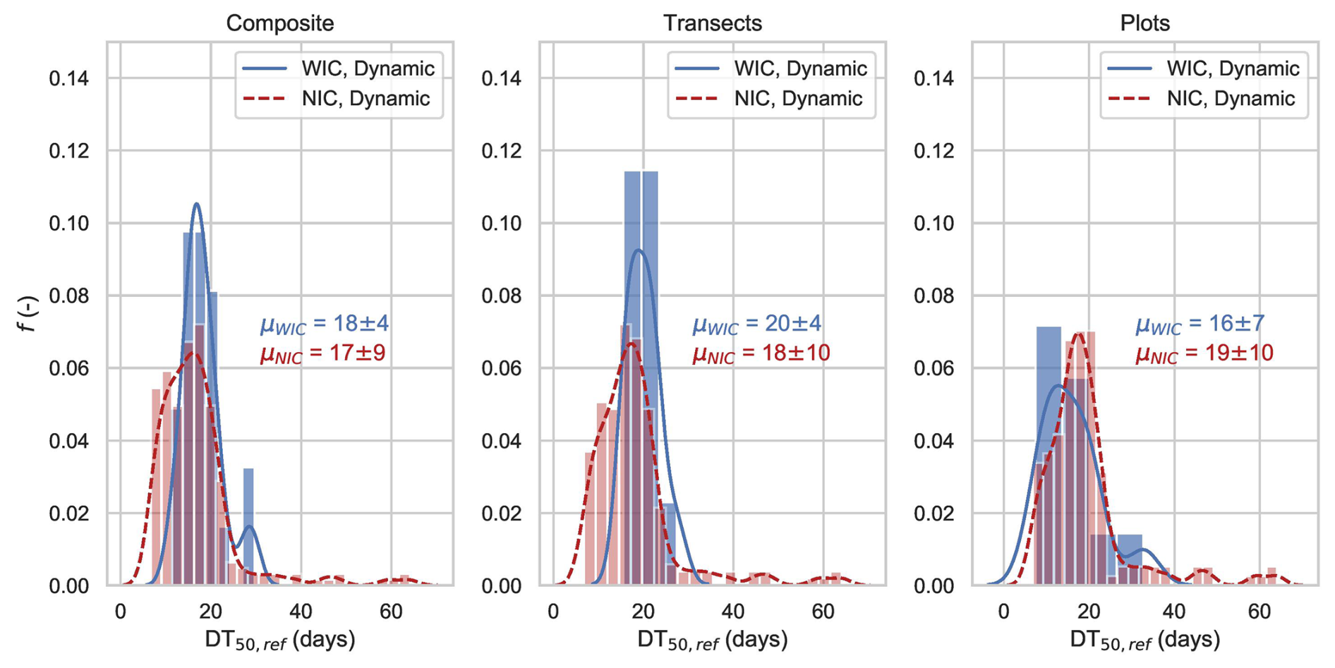
Figure 4 Distribution of calibrated DT₅₀ values for 2500 runs, shown for models without isotope constraints (NIC, n=672) and with isotope constraints (WIC, n=244) across three sampling resolutions: composite transect, transect, and plot-scale soils. NIC simulations were selected based on KGE_SM>0.5 and KGE_Q>0.5, while WIC simulation also included KGE_δ>0.8. Mean DT_50,ref distributions are indicated by solid (WIC) and dotted (NIC) lines, and standard deviations are reported as μ ± SD.

3.2 Uncertainty reduction through incorporation of CSIA data

This section underlines the benefit of incorporating topsoil CSIA data during model calibration (WIC, with isotope constraint) compared to no isotope constraint (NIC). For the composite transect soil (Fig. 4), the mean DT_50,ref values (μ; Eq. 8) were similar in the NIC and WIC calibrations. However, the standard deviation of DT_50,ref was twice as large for NIC, indicating significantly higher uncertainty. This demonstrates that including CSIA data in the calibration phase substantially reduced the uncertainty in S-metolachlor degradation estimates.

Reducing uncertainty in estimates of pesticide degradation in soil during the calibration of reactive transport models is crucial, as degradation half-lives can vary by 1 order of magnitude depending on the compound (Wang et al., 2018), which is largely affected by hydro-climatic and soil conditions. In this study, the WIC calibration yielded mean DT_50,ref below 20 d, with low standard deviations (SDs<7 d; Fig. 4) indicating that aerobic degradation of S-metolachlor, typically reported between 14 and 21 d (Lewis et al., 2016), was the dominant process in Alteckendorf topsoil. In contrast, anaerobic degradation, characterised by longer half-lives (DT₅₀=23–62 d; Seybold et al., 2001; Long et al., 2014), appeared to play a limited role.

The mean calibrated DT_50,ref values for transect composite soil, for individual transects across the catchment, and for plot resolutions differed by less than 4 d (Fig. 4). However, standard deviations reflecting uncertainty were approximately 50 % lower when isotopic constraints (WIC) were applied compared to calibrations without isotopic constraints (NIC) for both transect composite and transect-scale data. At the plot scale, uncertainty remained unchanged. These results indicate that increasing resolution (plots > transects > transect composite samples) did not significantly improve model calibration in this catchment. Therefore, pooling transect samples into a single composite soil sample was sufficient for CSIA-based calibration, while also reducing sampling and analytical efforts. This approach may reliably capture variations in pesticide degradation at the catchment scale.

Integration of CSIA data into PiBEACH yielded an isotope fractionation factor of $\mathit{\epsilon }C=-\mathrm{2.7}$ ‰ ± 0.6 ‰ for S-metolachlor degradation in topsoil, exceeding previously reported values (Alvarez-Zaldivar et al., 2018: −1.5 ‰ ± 0.5 ‰; Lutz et al., 2017: −1.3 ‰ ± 0.5 ‰). This discrepancy likely reflects differences in environmental conditions, microbial activity, and transformation pathways, although it remains within the model ensemble's uncertainty range. Compared to laboratory-derived estimates, the stronger fractionation observed suggests either alternative degradation pathways or the influence of distinct microbial consortia at the catchment scale, relative to laboratory conditions. These findings underscore the importance of site-specific calibration for CSIA applications and highlight the value of model ensemble approaches for capturing the range of degradation processes in heterogeneous agro-ecosystems. While previously reported εC values may slightly overestimate degradation in some field settings, the calibration of ensemble modelling with integrated CSIA data provides a more robust and field-relevant assessment of pesticide transformation. However, these findings necessitate further confirmation with a validation dataset, which was not available for the targeted catchment.

3.3 Metrics of pesticide persistence and transport risks

Six metrics were derived from calibrated PiBEACH outputs to evaluate S-metolachlor persistence in soil and its transport risk via leaching and runoff from topsoil across the catchment. Each metric was expressed as a percentage of applied S-metolachlor and included (i) S-metolachlor degradation (Fig. 5a), (ii) the remaining bioavailable mass (BAM) of S-metolachlor in topsoil (i.e. dissolved and reversibly sorbed S-metolachlor; Fig. 5b), (iii) the remaining mass of irreversibly sorbed S-metolachlor (aged; Fig. 5e), (iv) off-site transport of S-metolachlor by leaching (Fig. 5d), (v) S-metolachlor volatilisation (Fig. 5f), and (vi) S-metolachlor export to the catchment outlet by runoff and drainage (Fig. 5c). All metrics were calculated from the first application on 19 March (day 0) to 12 July 2016 (day 115). For two metrics, degradation and the remaining mass in topsoil, PiBEACH closely matched observations (Fig. 5a and b and Sect. S4 in the Supplement). The modelled degradation extent (72 % ± 13 %) was consistent with the value derived from δ¹³C measurements of composite transect soil and the Rayleigh equation (68 % ± 1 %) on day 87, corresponding to the last quantifiable soil isotope measurement (Fig. 5a). By day 115, the modelled degradation constituted the primary component of the mass balance, accounting for 82 % ± 21 % of the applied S-metolachlor mass. The remaining bioavailable mass (BAM) was estimated from measured concentrations and transect areas (Figs. 1 and S1). The extrapolated remaining BAM from the transect composite soil was 12 % ± 8 %, which fell within the modelled range at day 115 (18 % ± 3 %). The model slightly overestimated the export of S-metolachlor in the river to the outlet (2 % ± 6 %) in comparison to the observed values (0.5 % ± 0.1 %), which were not used during calibration. However, this difference remains within the model's uncertainty range. It is important to note that the observed exports were based solely on the dissolved phase, as particulate-bound S-metolachlor (>0.7 µm) remained below the quantification limits in all river water samples. The S-metolachlor export metric depends on PiBEACH's ability to simulate daily discharge. Although PiBEACH was originally designed to initialise sub-hourly event-based distributed models like OLP (Commelin et al., 2024), it also demonstrated a reasonable ability to reproduce daily discharge dynamics (Fig. 3b), consistent with prior applications in similar catchments (Sheikh et al., 2009). Finally, the S-metolachlor volatilisation predicted was low (<1 %) during the first 120 h after application, in line with the low vapour pressure of S-metolachlor (=1.7 mPa, Lewis et al., 2016). However, volatilisation rates ranging from 5 % to 63 % of the applied mass have been reported under variable meteorological conditions (Gish et al., 2011).

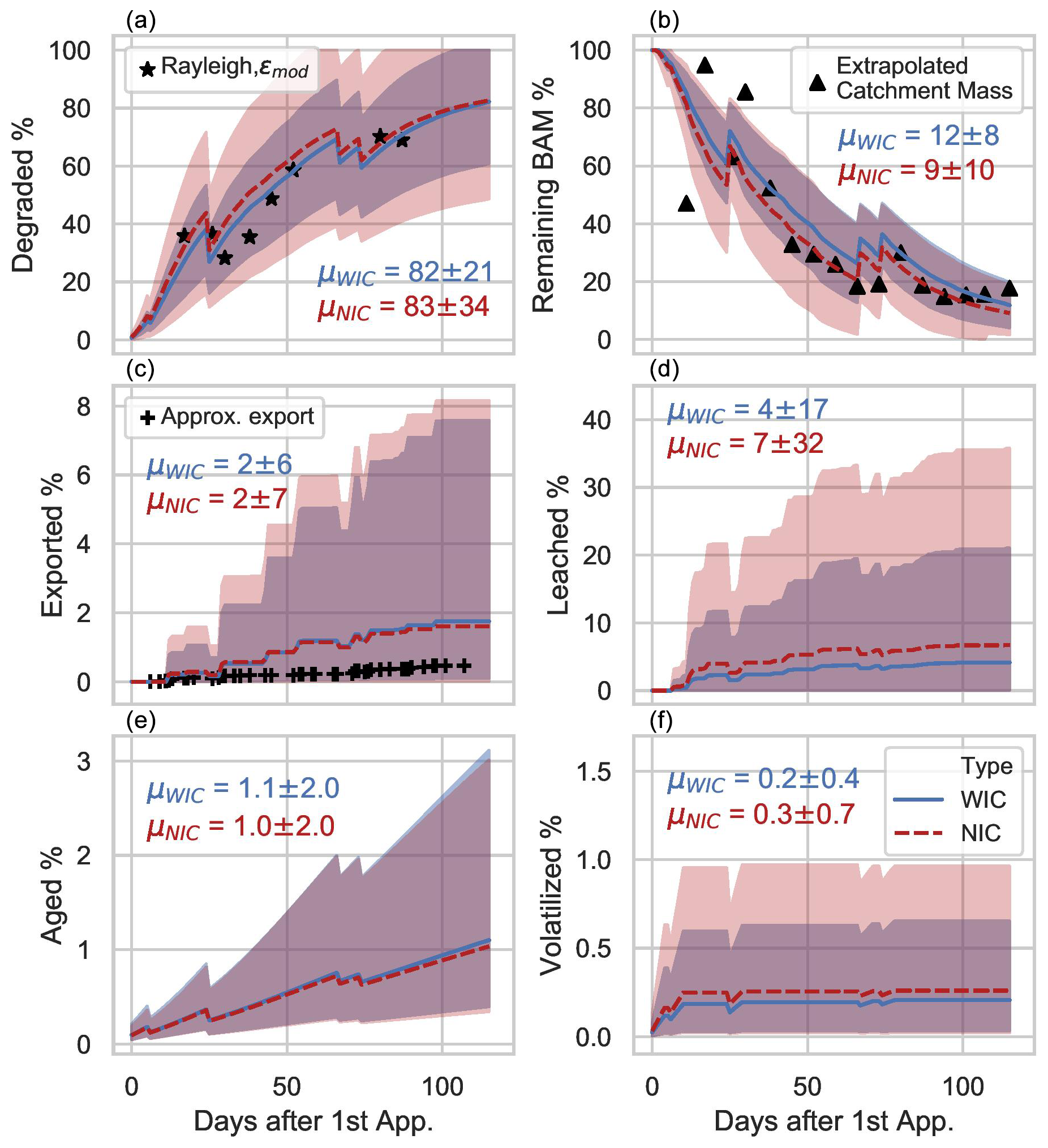
Figure 5 Pesticide dissipation processes and the corresponding ensemble mean from a total of 672 simulations without isotope constraints (NIC, dotted line) and 244 simulations with isotope constraints (WIC, solid line). The 95 % confidence intervals (CIs) are shown in red for NIC and blue for WIC. All metrics are expressed as percentages of the applied cumulative S-metolachlor mass across the catchment, starting from the first application on 19 March 2016. Final dissipation values (μ_WCI and μ_NIC ± 95 % CI) are reported for day 115. Black markers indicate estimates derived from catchment-scale mass balances based on farmer surveys (Sects. S3 and S4 in the Supplement).

The six pesticide transport metrics confirmed that incorporating CSIA data reduced the uncertainty in degradation estimates and in other dissipation processes simulated by the PiBEACH model. Comparison of the 95 % confidence intervals showed that, by the end of the season (day 115), uncertainty was reduced by half in the WIC ensemble (with CSIA data) compared to in the NIC ensemble (without CSIA data). Although the mean S-metolachlor degradation was similar for both dynamic DT₅₀ models at the end of the season (i.e. Δμ=1 %), the uncertainty around the degradation extent was 60 % higher in the NIC ensemble. The higher uncertainty propagated to other processes; for example, both the mean and uncertainties in S-metolachlor leaching were twice as high in the NIC simulations compared to those in WIC. The wide 95 % confidence intervals observed for the six metrics suggest that the thresholds used for the objective function, particularly KGE_SM>0.5 and KGE_Q>0.5, may need to be increased to reduce uncertainty. As previously noted in the application of the GLUE method (Jin et al., 2010), selecting an optimal threshold is inherently challenging, as it involves a trade-off between the computational effort required to retain a sufficient number of acceptable simulations and the resulting width of the confidence intervals.

This modelling framework, applied to the same compound and catchment as in Lutz et al. (2017), provides insights into the benefits and limitations of using δ¹³C data from soil and river samples to constrain reactive transport models. The lumped model by Lutz et al. (2017) focuses on δ¹³C values at the catchment outlet, providing an integrated signature of degradation processes across the catchment. In contrast, PiBEACH allowed for evaluation of the added value of topsoil δ¹³C data to constrain degradation kinetics. Model predictions for three components of the S-metolachlor mass balance, i.e. degraded mass, the remaining mass in topsoil, and export at the outlet, were validated against observations. Due to limitations representing the rapid surface off-site transport associated with runoff and erosion, PiBEACH did not incorporate δ¹³C data from rivers into the calibration. However, future coupling of PiBEACH with an event-based model like OLP could enable simultaneous integration of both topsoil and river δ¹³C datasets, improving constraints on degradation and enhancing simulation of fast-flow transport during high-intensity rainfall–runoff events.

In summary, δ¹³C data from both soil and river samples can enhance model calibration by constraining degradation processes along different transport pathways. Lumped models (e.g. Lutz et al., 2017) and distributed models like PiBEACH each offer complementary perspectives on pesticide dynamics. However, only a distributed model can account for spatial heterogeneity across the catchment and support management decisions. PiBEACH also provides spatially explicit outputs of pesticide concentrations, hydraulic properties, and topsoil moisture as critical inputs for initialising distributed event-based models. A large portion of the outlet data, i.e. discharge for calibration (as part of the KGE objective function), discharge, and S-metolachlor concentrations to evaluate export, was used to assess model performance. Nevertheless, due to limitations of PiBEACH's conceptual structure and daily resolution, the comparison between observed and simulated reactive transport was limited, unlike previous lumped approaches (Lutz et al., 2017). The forthcoming PiBEACH–OLP modelling effort will explore the added value of incorporating observed S-metolachlor concentrations and isotopic signatures at the outlet into the calibration process.

This study demonstrates that even a moderate sampling effort, including weekly CSIA measurements from composite topsoil samples across the catchment, can effectively identify hotspots and hot moments of pesticide degradation at the catchment scale. In PiBEACH, degradation is primarily driven by soil temperature and moisture, which exhibits clear seasonal and vertical gradients. As a result, degradation hotspots were consistently located in the topsoil. In contrast, soil moisture, although more spatially variable than temperature, played a secondary role. No significant spatial differences in DT₅₀ were observed among plots treated with S-metolachlor over the growing season. The limited spatial variation in simulated DT₅₀ across the catchment does not diminish the value of PiBEACH's distributed nature, particularly when considering its future integration with distributed event-based models such as OLP. This coupling remains essential for simulating surface transport during rainfall events and for refining predictions of pesticide fate under dynamic hydrological conditions.

As the field of pesticide CSIA evolves through multi-element CSIA applications (Torrentó et al., 2021; Höhener et al., 2022) and the development of passive sampling techniques (Gilevska et al., 2022a), the ability to evaluate dissipation processes and distinguish between competing pathways (Elsner and Imfeld, 2016; Hofstetter et al., 2024) will enhance assessments of pesticide degradation in agricultural soils and enable more robust catchment-scale modelling.

4 Conclusion

This study addresses the gap between the increasing complexity of reactive transport models and the limited availability of field data for their calibration. Although the representation of interactions between hydro-climatic conditions, biogeochemical processes, and degradation dynamics has improved significantly in recent decades, it remains oversimplified in many 2D catchment models (Lutz et al., 2013) or is not explicitly defined (DeMars et al., 2018). Incorporating more detailed physical and biological representations of degradation in catchments increases model complexity and uncertainty, making it essential to acquire additional data to constrain parameter ranges and reduce equifinality. Our findings suggest that using only topsoil pesticide concentrations and discharge measurements is insufficient to effectively constrain reactive transport models at the catchment scale. We demonstrated that incorporating complementary data, such as pesticide CSIA data (Fenner et al., 2013; Elsner and Imfeld, 2016; Hofstetter et al., 2024), can help differentiate between degradative and non-degradative processes that contribute to observed concentration declines. In many cases, carbon isotope data (δ¹³C) alone may be adequate to provide evidence of in situ degradation, thereby supporting pesticide mass balance closure and improving model calibration at the catchment scale. The next step should involve confirming these findings with a validation dataset, which was not available for the targeted catchment. Looking ahead, multi-element CSIA has the potential to further elucidate competing degradation pathways (Höhener et al., 2022). To improve model accuracy, future research should also consider the dynamics of microbial functional diversity, biomass, and biodegradation potential (König et al., 2018).

Our results highlight the potential of topsoil CSIA data to inform pesticide management strategies by providing more reliable estimates of degradation and transport processes at the headwater catchment scale. Given the strong effect of hydro-climatic factors on pesticide degradation and transport, especially under the changing rainfall and temperature regimes driven by climate change (Barrios et al., 2020), it is essential to account for these dynamics in pesticide fate assessments. Furthermore, risk metrics for pesticide risk assessment often require probabilistic approaches, including confidence intervals (Lutz et al., 2013). Therefore, to support decision-making and eco-toxicological assessments, hydrological models should systematically incorporate uncertainty frameworks to capture the full range of parameter values affecting pesticide transfer risks.