An efficient hybrid downscaling framework to estimate high-resolution river hydrodynamics

Flow depth and velocity are the most important hydrodynamic variables that govern various river functions, including water resources, navigation, sediment transport, and biogeochemical cycling. Existing high-resolution flow depth simulations rely on either computationally expensive river hydrodynamic models (RHMs) or data-driven models with formidable training costs, whereas data-driven modeling of flow velocity has rarely been explored. Here, using the hybrid Low-fidelity, Spatial analysis, and Gaussian process learning (LSG) model, we developed a downscaling approach to construct high-resolution flow depth and velocity from a two-dimensional (2-D) RHM simulation at coarse resolution. The LSG models were trained and tested in an urban watershed in Houston using two different hurricane-driven flood events. The high-resolution (as fine as 30 m resolution) and low-resolution (mostly 1000 m resolution) meshes include 664 724 and 14 536 grid cells, respectively. The results showed that through downscaling, the simulation errors were reduced to less than one-fourth and one-third of the errors of the low-resolution 2-D RHM for flow depth and velocity, respectively. Our analysis further revealed that the dominant uncertainty sources of the downscaled hydrodynamics are different, with flow velocity dominated by the dimensionality reduction error, which we reduced by using a regionalized training procedure. The downscaling approach achieves an 84-fold acceleration in computational time compared to the high-resolution 2-D RHM, making high-fidelity ensemble flood modeling feasible. More importantly, the developed method provides an opportunity to couple large-scale hydrodynamical processes with local physical, chemical, and biological processes in river models.

1 Introduction

Rivers play a crucial role in water resources, navigation, sediment transport, and biogeochemical cycling (Syvitski et al., 2005; Oki and Kanae, 2006; Allen and Pavelsky, 2018; Ibáñez and Peñuelas, 2019; Mao et al., 2019; Regnier et al., 2022; Feng et al., 2023a; Rocher-Ros et al., 2023). To sustain these vital services, river flow depth and velocity must remain within normal ranges. Extreme flow depths can result in extensive fluvial flooding (Bates, 2022), whereas prolonged low flow depths jeopardize the availability of drinking and irrigation water in many regions worldwide (Gadgil, 1998; Haddeland et al., 2006). Together, flow depth and velocity are key drivers of navigation capability, sediment transport, and biogeochemical processes in rivers (Zhang et al., 2014; Raymond et al., 2016; Li et al., 2022; Sukhodolov et al., 2023). Consequently, extreme variations in flow depth and velocity can lead to waterway blockage, channel aggradation or degradation, water quality deterioration, and habitat loss. River flow depth and velocity regimes are dynamic and influenced by climate change and human activities, leading many rivers to experience extreme flow conditions (Mishra and Shah, 2018). These conditions exacerbate flooding (Freer et al., 2011), degrade aquatic ecosystems (Carpenter et al., 2011; Battin et al., 2023), and diminish water supplies (Oki and Kanae, 2006). Hence, accurate prediction of river flow depth and velocity in the context of a changing climate is essential for ensuring the well-being of human society (IPCC, 2021).

Flow depth and velocity are commonly simulated using river hydrodynamic models (RHMs). Widely used RHMs are often based on one-dimensional (1-D) or two-dimensional (2-D) Saint-Venant equations, disregarding vertical variations due to the significant difference between the horizontal and vertical length scales of rivers (Li et al., 2013; Teng et al., 2017; Bates, 2022; Huang et al., 2022). Considering the low computational cost and high numerical stability, Earth system models (ESMs) usually employ 1-D RHMs as the river component for large-scale and/or ensemble hydrological simulations (Li et al., 2013; Feng et al., 2024). However, they are unsuitable for high-fidelity flood simulations. This is because 1-D RHMs are solved on upscaled river networks rather than actual river reaches (Wu et al., 2011; Liao et al., 2022) and rely on uncertain parameterizations, such as the bathtub method for estimating floodplain inundation (Luo et al., 2017; Xu et al., 2022). Additionally, by oversimplifying and/or neglecting momentum transport in river channels and floodplains (Luo et al., 2017; Feng et al., 2022), 1-D RHMs lack the capability to simulate fine-scale river hydrodynamics required for geomorphological and biogeochemical modeling (Hostache et al., 2014; Shabani et al., 2021). Conversely, 2-D RHMs can solve full river dynamics. When running on high-resolution meshes, they can accurately capture river flow depth and velocity (Razavi et al., 2012). Therefore, high-resolution 2-D RHMs are often referred to as high-fidelity (HF) models, whereas both 1-D RHMs and low-resolution 2-D RHMs are referred to as low-fidelity (LF) models. However, the significant computational cost of HF RHMs (Teng et al., 2017; Wu et al., 2020; Ivanov et al., 2021) makes them not viable for real-time modeling and flood risk assessments through ensemble modeling, which requires hundreds or thousands of model realizations (Wu et al., 2020).

To achieve accurate and affordable simulations of river hydrodynamics, several alternative approaches have been developed (Razavi et al., 2012). One prominent approach is the use of data-driven models to emulate the behaviors of HF RHMs (Ivanov et al., 2021; Tran et al., 2023). With the rapid advancement of machine learning (ML) techniques, ML-based emulators have been increasingly employed in hydrological sciences, including applications such as modeling runoff (Gao et al., 2020), evapotranspiration (Hu et al., 2021), inundation (Xie et al., 2021), lake–river interactions (Liang et al., 2018; Huang et al., 2022), reservoir operations (Zhang et al., 2018; Yang et al., 2019b), streamflow (Ha et al., 2021; Sikorska-Senoner and Quilty, 2021), groundwater (He et al., 2020; Wunsch et al., 2022), and water quality (Chen et al., 2020; Saha et al., 2023). These studies have demonstrated that, once trained under extensive conditions, the computationally efficient ML models can mimic numerical models. However, general ML-based emulators often lack the enforcement of physical laws, such as the conservation of mass and momentum (Konapala et al., 2020; Karniadakis et al., 2021), resulting in poor transferability to out-of-sample conditions in nonstationary systems (Young et al., 2017; Konapala et al., 2020), such as streamflow in a changing climate. To address this limitation, variants like physics-informed neural networks have been developed, embedding physical laws (e.g., Saint-Venant equations) into their cost functions to constrain ML solutions. However, the incorporation of physical laws tends to reduce the training efficiency of ML models (Feng et al., 2023b).

The second approach is to downscale the low-resolution RHM simulation onto a finely discretized grid (Wilby and Dawson, 2013; Feng et al., 2023b). For instance, Bermúdez et al. (2020) created high-resolution inundation maps by simply interpolating flow depth computed from an LF RHM onto a high-resolution digital elevation model (DEM). Recently, more advanced downscaling methods have been developed using various ML techniques to reproduce the detailed spatial and temporal features of high-resolution river hydrodynamics (Carreau and Guinot, 2021). Notably, Fraehr et al. (2022) developed a novel downscaling method based on the hybrid Low-fidelity, Spatial analysis, and Gaussian process learning (LSG) model. This method demonstrated promising accuracy in simulating the dynamic behavior of flood inundation, such as the rising and recession components and hysteresis, at the computational cost of a low-resolution 2-D RHM (Fraehr et al., 2022). Later, Fraehr et al. (2023a) extended the approach for fast and accurate simulations of not only high-resolution flood extent but also high-resolution flow depth. Additionally, the LSG-based downscaling model can support both structured and unstructured grids, a significant advantage as modern 2-D RHMs increasingly adopt unstructured grids for fine-scale modeling (Begnudelli and Sanders, 2006; Kim et al., 2012). However, like Fraehr et al. (2022, 2023a), existing research on hydrodynamic model downscaling is mostly flood-prediction-oriented and has thus focused entirely on flood extent and magnitude, while ignoring flow velocity. This oversight is problematic from two perspectives. First, it could increase the uncertainty of flood risk simulations because flood velocity is a critical factor for human safety risks in flood events (Russo et al., 2013). Moreover, as discussed earlier, in the context of Earth system modeling, without accurate simulations of flow velocity, it is not possible to realistically predict how river functions respond to environmental stresses. While Fraehr et al. (2022, 2023a) only applied the LSG-based downscaling approach for inundation extent and depth, this method should theoretically also be applicable for flow velocity. This is because the mass and momentum of river flow are governed by the unified shallow water equations and driven by the same environmental factors. However, such an application has not yet been explored.

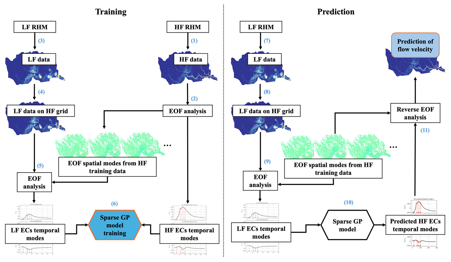
Figure 1 Workflow of training the LSG model and using the trained model to predict high-resolution river hydrodynamics.

In this study, we develop an LSG-based downscaling approach to achieve accurate simulations of high-resolution river flow depth and velocity at the computational cost of a low-resolution 2-D RHM. Compared to Fraehr et al. (2022, 2023a), the main innovation of our study is to test and enhance the LSG-based downscaling approach for high-resolution flow velocity downscaling. This extension of the LSG-based downscaling approach is expected to greatly broaden its usefulness for Earth system modeling. Besides, we test the effectiveness of the downscaling method in an urbanized watershed in the Houston area using data from two different extreme hurricane events. Together with Fraehr et al. (2022, 2023a), our independent validation in a different environment would help examine whether the LSG-based downscaling approach has broad geographical applicability. Furthermore, based on this downscaling method, we propose a new paradigm to couple large-scale hydrodynamical processes with local detailed physical, chemical, and biological processes in river models. The remainder of this paper is organized as follows: Sect. 2 describes the downscaling method and the configurations of the high-resolution and low-resolution 2-D RHMs for the study events; Sect. 3 highlights the main results; Sect. 4 discusses the implications of the results, outlines the limitations of our approach, and introduces the new paradigm; and Sect. 5 concludes the paper.

2 Materials and methods

2.1 LSG model

For the LSG model, the underlying principle is that the dynamics of flow depth and velocity can be approximated by a limited number of temporal and spatial modes due to their strong spatial pattern controlled by topography. The LSG model consists of an LF RHM, key spatial modes extracted from an HF RHM, and a sparse Gaussian process (GP) emulator model. It uses the LF RHM as a transfer function to capture the dynamics and spatial correlation of river flow. The key temporal features of the LF RHM outputs are extracted through an empirical orthogonal function (EOF) analysis based on the extracted spatial features from the HF RHM, thereby allowing the use of a sparse GP model to convert the LF data to HF data via conversion of the extracted temporal features. The LSG model can reconstruct high-fidelity river hydrodynamics for two reasons. First, the accurate spatial correlations of river hydrodynamics are preserved due to the use of the key spatial modes from the HF model, which are assumed not to vary by event. Second, the sparse GP model is efficient and effective in reconstructing the dynamics of HF data. In this study, we used the same 2-D shallow water equations to construct the LF and HF RHMs (described later). The only difference between them is the spatial resolution, with the coarse mesh adopted by the LF model reducing the simulation accuracy. We followed the procedure described by Fraehr et al. (2022, 2023a) to train and apply LSG models for river flow depth and velocity downscaling (Fig. 1), with any deviations from the general procedure specifically highlighted.

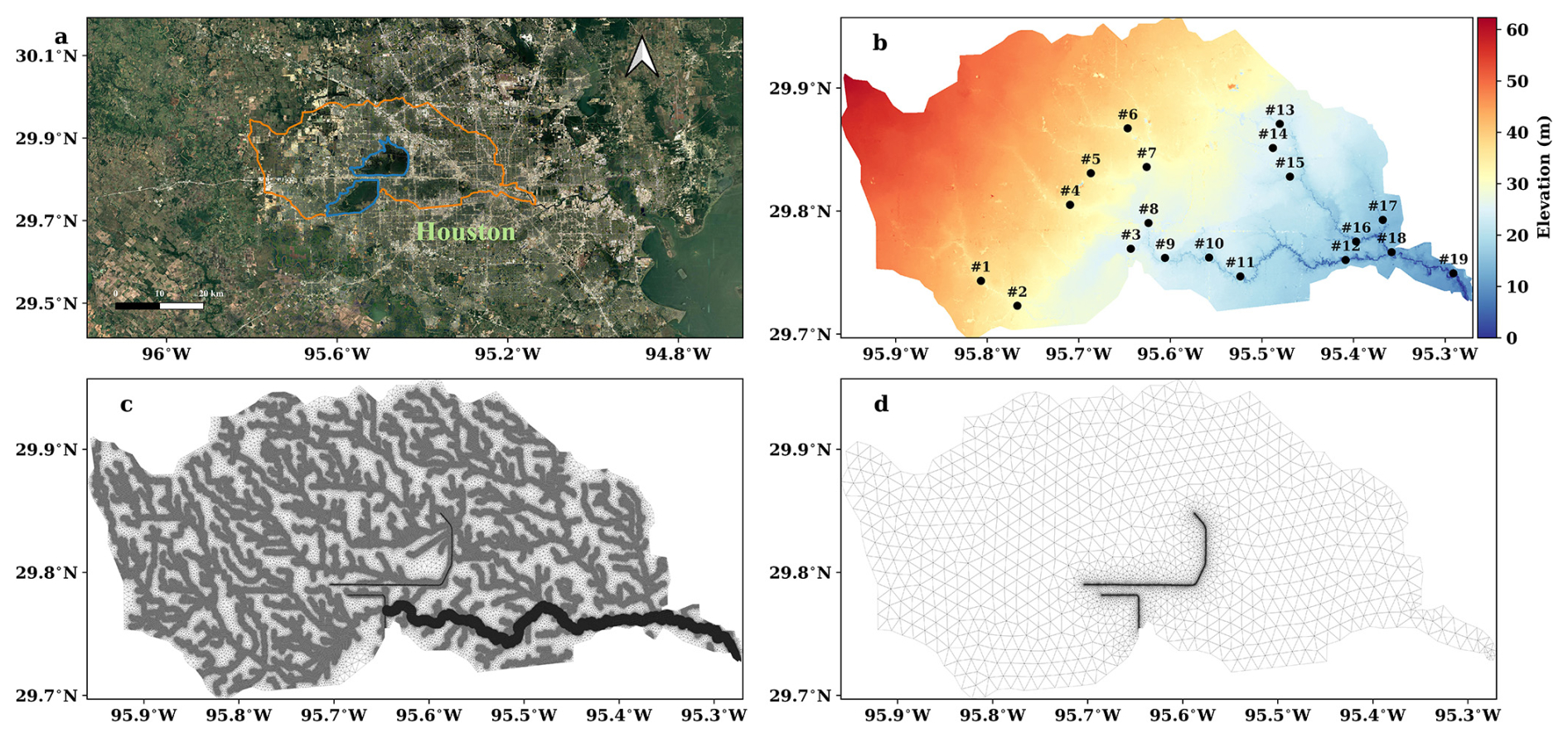
Figure 2 Study domain (a), topography (b), high-resolution mesh (c), and coarse-resolution mesh (d) for river hydrodynamics simulations in the Turning River basin. The river basin boundary and the boundaries of two reservoirs in the basin are highlighted in orange and blue, respectively, in (a), and the black dots in (b) show the locations of the USGS gauges (Table S1 in the Supplement) along with their gauge number. The basemap in (a) is extracted from Google Imagery© 2024 TerraMetrics, Map data© 2024. The seemingly thick bold lines in (c) are dense grid cells for river channels. The seemingly black lines in (d) are dense grid cells for the dams of the two reservoirs, which can also be seen in (c).

For training, we first run the HF RHM over the study domain for a training flood event (Step 1) and derive the spatial EOF modes and the temporal expansion coefficient (EC) modes of this HF simulation through the EOF analysis (Step 2) as defined in Eq. (1).

$$\begin{array}{}\text{(1)}& {\mathbf{D}}_{\text{HF}}={\mathbf{U}}_{\text{HF}}\cdot {\mathbf{C}}_{\text{HF}}\approx {\sum }_{k=\mathrm{1}}^K{\mathbf{U}}_{\text{HF}}(k,:)\cdot {\mathbf{C}}_{\text{HF}}(:,k),\end{array}$$

where D_HF is a T × N matrix containing simulated HF flow depth or velocity (T is the number of time steps in the training data and N is the number of wet cells) that have been detrended (Fraehr et al., 2023a), U_HF is a T × N matrix, each row of which is an EOF spatial map, C_HF is a T × T matrix, each column of which corresponds to an EC temporal function, and K is the number of significant modes determined by both North's test (North et al., 1982) and Kaiser's rule (Kaiser, 1960).

For the training phase, we also run the LF RHM for the training event (Step 3) and interpolate the simulated flow depth and velocity from the coarse mesh used by the LF model to the fine mesh used by the HF model (Step 4). Notably, we improved the nearest-neighbor interpolation method adopted by Fraehr et al. (2023a) by accounting for mass conservation. While our improved method still assumes a homogeneous water level within a coarse grid cell, it ensures that the sum of interpolated water volume in fine grid cells equals the water volume in the coarse grid cell. Additionally, we ensure that the interpolation of flow velocity only occurs at wet grid cells where the water depth is greater than 3 cm (Fraehr et al., 2023a). Another difference is that we do not apply area-based weights to D_HF before the EOF analysis, as Fraehr et al. (2023a) recommended. This is because we are more interested in the flow depth and velocity of river channels and nearby floodplains that are represented by smaller grid cells in our fine mesh (Fig. 2).

Next, we perform the EOF analysis on the interpolated LF flow depth and velocity to derive the temporal EC modes of the LF simulation (Step 5). Using the extracted high-resolution EOF spatial modes from Step 2, the extracted temporal ECs are defined in Eq. (2).

$$\begin{array}{}\text{(2)}& {\mathbf{C}}_{\text{LF}}={\mathbf{D}}_{\text{LF}}\cdot {\mathbf{U}}_{\text{HF}}^{\prime },\end{array}$$

where C_LF is a T × T matrix containing the LF ECs, D_LF is a T × N matrix corresponding to the interpolated LF flow depth or velocity simulations, and ${\mathbf{U}}_{\text{HF}}^{\prime }$ is the transpose of U_HF. In the final step of training, we use the derived LF and HF temporal ECs to train a sparse GP model (Rasmussen and Williams, 2006) that can predict the HF ECs from the LF ECs (Step 6). For flow depth and velocity, the training of the sparse GP models is performed independently.

For prediction, only the low-cost LF RHM simulations are needed (Fig. 1). While Steps 7 to 9 essentially replicate Steps 3 to 5, the difference is that Steps 7 to 9 are applied to a new LF simulation that is run for an unseen flood event. After the new LF ECs are retrieved following the EOF analysis in Eq. (1) using the spatial EOF modes derived in Step 2, they are fed into the trained sparse GP model to predict the new HF ECs (Step 10). Finally, the predicted HF ECs are combined with the EOF spatial modes from Step 2 to reconstruct the HF flow depth and velocity simulations based on the reverse EOF analysis (Step 11) as defined in Eq. (3).

$$\begin{array}{}\text{(3)}& \widehat{{\mathbf{D}}_{\text{LSG}}}=\sum _{k=\mathrm{1}}^K{\mathbf{U}}_{\text{HF}}(k,:)\cdot \widehat{{\mathbf{C}}_{\text{LSG}}}(:,k),\end{array}$$

where $\widehat{{\mathbf{D}}_{\text{LSG}}}$ is the predicted high-resolution flow depth or velocity, and $\widehat{{\mathbf{C}}_{\text{LSG}}}$ is the predicted HF temporal EC. More details of the workflow can be found in Fraehr et al. (2022, 2023a).

The downscaling error consists of two major components: the error from dimensionality reduction and the error from the LSG model. According to Eq. (1), the error from dimensionality reduction ER_DR can be defined as ${\text{ER}}_{\text{DR}}={\mathbf{D}}_{\text{HF}}-{\sum }_{k=\mathrm{1}}^K{\mathbf{U}}_{\text{HF}}(k,:)\cdot {\mathbf{C}}_{\text{HF}}(:,k)$. According to Eq. (3), the error from the LSG model ER_LSG can be defined as ${\text{ER}}_{\text{LSG}}={\sum }_{k=\mathrm{1}}^K{\mathbf{U}}_{\text{HF}}(k,:)\cdot {\mathbf{C}}_{\text{HF}}(:,k)-\sum _{k=\mathrm{1}}^K{\mathbf{U}}_{\text{HF}}(k,:)\cdot \widehat{{\mathbf{C}}_{\text{LSG}}}(:,k)$.

2.2 Study site and flood events

We used the Hurricane Harvey flood event (hereafter referred to as Harvey) in the Houston area as a case study. On 26 August 2017, Harvey made landfall along the mid-Texas coast as a Category 4 hurricane. As one of the worst hurricanes to hit the United States in recent history, Harvey brought record-breaking rainfall across the Houston metropolitan area (Van Oldenborgh et al., 2017), causing more than 80 fatalities and over USD 150 billion in economic losses, mostly due to extraordinary flooding (Emanuel, 2017; Balaguru et al., 2018). Specifically, we selected the Buffalo Bayou at Turning Basin as the study domain (Fig. 2), where the selected RHM was recently validated at different resolutions (Xu et al., 2025).

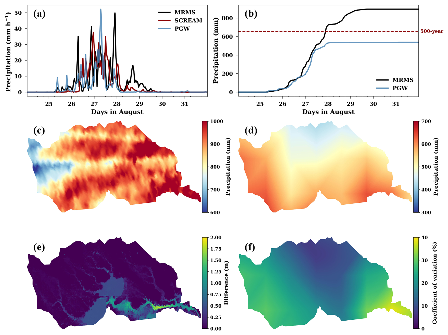
Figure 3 Comparison of the observed (MRMS) and simulated hourly precipitation during Harvey under the observed historical (SCREAM) and projected future (PGW) conditions (a), comparison of the cumulative MRMS and PGW precipitation (b), and maps of the observed cumulative precipitation during Harvey (c), the cumulative precipitation of the PGW simulation selected for the LSG model validation (d), the difference between the simulated peak water depth from the HF RHM using MRMS and that using the PGW precipitation (e), and the coefficient of variation (CV) of the PGW simulated cumulative precipitation ensemble (f) in the study domain. The 7 d total precipitation for the 500-year return period in the Houston area is marked in (b).

Precipitation during Hurricane Harvey (Fig. 3) is extracted from the 1 km resolution Multi-Radar Multi-Sensor (MRMS) precipitation dataset, which has a native temporal resolution of 2 min (Zhang et al., 2016). To demonstrate the effectiveness of our downscaling approach for ensemble flood projections, we use a projected hurricane event (Hurricane Harvey-like) under the high warming scenario – Shared Socioeconomic Pathway SSP5-8.5 – as a test case (Fig. 3). The future hurricane is simulated using the Energy Exascale Earth System Model (E3SM) with the novel Simple Cloud-Resolving E3SM Atmosphere Model (SCREAM) configuration (Caldwell et al., 2021; Donahue et al., 2024). SCREAM is a global atmospheric circulation model with a nonhydrostatic dynamical core and parameterizations for atmospheric radiative transfer, cloud microphysics, and boundary layer clouds and turbulence (Caldwell et al., 2021). The SCREAM domain features a regionally refined mesh (RRM) with 3.25 km grid spacing over the east coast of the United States, including the Gulf of Mexico and a significant part of the Atlantic Ocean, within a global domain that has 25 km grid spacing outside the RRM. Nudging is applied to grid cells outside the RRM to constrain the atmospheric circulation using the European Centre for Medium-Range Weather Forecasts (ECMWF) Reanalysis version 5 (ERA5) data (Hersbach et al., 2020). These features enable SCREAM to capture fine-scale extreme weather events, accurately resolve coastal areas and mountainous regions, and properly represent convective clouds, which are major sources of climate model uncertainty (Sherwood et al., 2014). SCREAM is coupled with the E3SM Land Model (ELM), while sea surface temperature and sea ice extent are prescribed based on ERA5.

In the historical simulation, SCREAM is initialized using ERA5 to simulate Hurricane Harvey (hereafter referred to as the SCREAM simulation). To simulate how Hurricane Harvey will behave under future conditions, a storyline simulation using SCREAM is performed (hereafter referred to as the Pseudo Global Warming, PGW, simulation). In the PGW simulation, the initial conditions and nudging data from ERA5 are perturbed by adding the mean monthly changes derived from a multi-model ensemble of climate simulations from the Coupled Model Intercomparison Project Phase 6 (CMIP6) to represent the mean climate change under the SSP5-8.5 scenario by the end of the 21st century (2079–2099) compared to the historical climate at the end of the 20th century (1990–2010). A similar perturbation is also applied to ELM for the PGW simulations.

SCREAM can successfully predict the heavy precipitation during Harvey's landfalls in Texas on 26 August, but its simulated precipitation during the subsequent landfalls on 27 and 28 August is relatively muted (Fig. 3a), a well-known challenge even for many weather forecasting models (Wang et al., 2018; Yang et al., 2019a). Considering the high computational cost of the SCREAM runs, we conducted three PGW simulations to drive the ensemble flood projections. These simulations, each with slightly different initial conditions, represent the uncertainty of the hurricane projection due to internal variability at the weather timescale (Fig. 3f). One PGW simulation is selected for LSG model validation. Its temporal and spatial patterns of precipitation are shown in Fig. 3a, b, and d, which are significantly different from the patterns of the benchmark precipitation (Fig. 3a–c) selected for LSG model training. The simulation differences reflect model uncertainty and the effects of climate change on the hurricane. Correspondingly, the simulated peak water depth from the HF RHM using the benchmark precipitation is significantly larger than that using the PGW precipitation (Fig. 3e). The significant difference in the benchmark and PGW precipitation as well as that in flood simulations supports the use of the latter as an out-of-sample test case, relevant for projecting future flooding. Additionally, the choice of a PGW flood event over a historical flood event for validation aligns better with the application scenarios of our downscaling method that are ensemble flood projections.

2.3 River hydrodynamic model

In this study, we chose the 2-D Overland Flow Model (OFM; Kim et al., 2012) for river hydrodynamics modeling, which was recently validated for the Harvey flood simulations (Xu et al., 2025). Briefly, OFM is a finite-volume model that implements the first-order Godunov-type upwind scheme on a triangular mesh and uses Roe's approximate Riemann solver to compute fluxes between grid cells (Begnudelli and Sanders, 2006). Later, Ivanov et al. (2021) improved OFM's computational efficiency by using the Portable, Extensible Toolkit for Scientific Computation (PETSc; Balay et al., 2019) software for model parallelization. Mathematically, OFM solves the 2-D shallow water equations, which include the terms of advection, bottom friction, and gravity but ignore the terms of Coriolis and viscous forces (Begnudelli and Sanders, 2006):

$$\begin{array}{}\text{(4)}& {\displaystyle \frac{\partial h}{\partial t}}+{\displaystyle \frac{\partial \left(uh\right)}{\partial x}}+{\displaystyle \frac{\partial \left(vh\right)}{\partial y}}=q,\text{(5)}& {\displaystyle }\begin{array}{rl}{\displaystyle \frac{\partial \left(uh\right)}{\partial t}}& +{\displaystyle \frac{\partial \left(u^{\mathrm{2}}h+\frac{\mathrm{1}}{\mathrm{2}}g{h}^{\mathrm{2}}\right)}{\partial x}}\\ & +{\displaystyle \frac{\partial \left(uvh\right)}{\partial y}}=-gh{\displaystyle \frac{\partial z_{\mathrm{b}}}{\partial x}}-C_{\mathrm{D}}u\sqrt{u^{\mathrm{2}}+v^{\mathrm{2}}},\end{array}\text{(6)}& {\displaystyle }\begin{array}{rl}{\displaystyle \frac{\partial \left(vh\right)}{\partial t}}& +{\displaystyle \frac{\partial \left(uvh\right)}{\partial x}}\\ & +{\displaystyle \frac{\partial \left(v^{\mathrm{2}}h+\frac{\mathrm{1}}{\mathrm{2}}g{h}^{\mathrm{2}}\right)}{\partial y}}=-gh{\displaystyle \frac{\partial z_{\mathrm{b}}}{\partial y}}-C_{\mathrm{D}}v\sqrt{u^{\mathrm{2}}+v^{\mathrm{2}}},\end{array}\end{array}$$

where t is the time (s), h is the flow depth (m), u and v are the water velocity (m s⁻¹) in the x and y direction under the Cartesian coordinate system, q is the excess precipitation rate (m s⁻¹), g is the gravitational acceleration constant (m s⁻²), z_b is the bed elevation (m), and C_D is the bed drag coefficient derived from Manning's roughness n as $C_{\mathrm{D}}=g{n}^{\mathrm{2}}{h}^{-\mathrm{1}/\mathrm{3}}$.

We configure the OFM model on two variable-resolution meshes, with the high-resolution configuration serving as the HF RHM and the low-resolution configuration as the LF RHM. The variable-resolution meshes are generated using a Delaunay-based unstructured mesh generator, JIGSAW (Engwirda, 2017), which can refine topographic features important for shaping river flow regimes, such as river channels (Kim et al., 2022; Xu et al., 2022), floodplains (Yamazaki et al., 2011; Schrapffer et al., 2020), and water management structures (Schmutz and Moog, 2018). Specifically, the high-resolution mesh has 664 724 grid cells over the study domain, representing the main channels, tributaries, dams, and other regular cells with resolutions of 30, 60, 30, and 1000 m, respectively. In contrast, the low-resolution mesh has only 14 536 grid cells over the study domain, representing the main channels, tributaries, and other regular cells with a uniform resolution of 1000 m (except for dams, which are resolved at 30 m) (Fig. 2). In both the high-resolution and low-resolution meshes, the areas around two flood control reservoirs, Addicks and Barker's Reservoir (Fig. 2), are refined to ensure more accurate flood simulations. As indicated in Xu et al. (2025), even though the simulation of streamflow at the outlet is only moderately degraded, the use of a coarser mesh severely deteriorates the model performance in simulating inundation. The 30 m resolution digital elevation model (DEM) from the National Elevation Database (NED) was used to construct the topography of the RHM meshes.

To force the OFM, the MRMS precipitation data are upscaled from their native temporal resolution to an hourly time step and spatially interpolated to the variable-resolution mesh cells using the nearest-neighbor interpolation method. Similarly, the hourly SCREAM simulation data are spatially interpolated to the variable-resolution mesh cells using the nearest-neighbor method before being used to force the OFM.

2.4 Validation of downscaled hydrodynamics

Validation of the downscaling method uses the “perfect prognosis” approach in which the HF RHM simulation is the target for the downscaled flow depth and velocity that uses the LF RHM simulated flow depth and velocity as the input. This validation strategy allows one to focus on evaluating the downscaling method without the influence of the RHM or observation errors and has been widely adopted in climate downscaling (Denis et al., 2002) as well as hydrological and hydrodynamic downscaling (Carreau and Guinot, 2021; Feng et al., 2023b) when both low- and high-resolution simulations are available. Therefore, in this study, good agreement between the downscaled flow depth and velocity with the high-resolution simulations from the HF RHM is a demonstration of the effectiveness of the downscaling method.

In the study, the accuracy of the downscaled hydrodynamics is evaluated using multiple metrics. Using the HF simulation as the reference, we calculate the root mean square error (RMSE) of the simulated hourly flow depth and velocity at each grid cell during the flood event and the absolute bias of the simulated flow depth and velocity at each grid cell during the flood peak. These two metrics are used to evaluate the spatial uncertainty of the downscaled estimates. The average RMSE of all the grid cells is also calculated to highlight the overall uncertainty of the downscaling. The temporal uncertainty of the downscaled hydrodynamics is assessed using the Kling–Gupta efficiency (KGE) (Gupta et al., 2009), which can evaluate the bias, correlation, and error variability of the downscaling comprehensively. The KGE is calculated at 19 USGS gauges (Fig. 2), which have been previously used to validate the HF RHM (Xu et al., 2025).

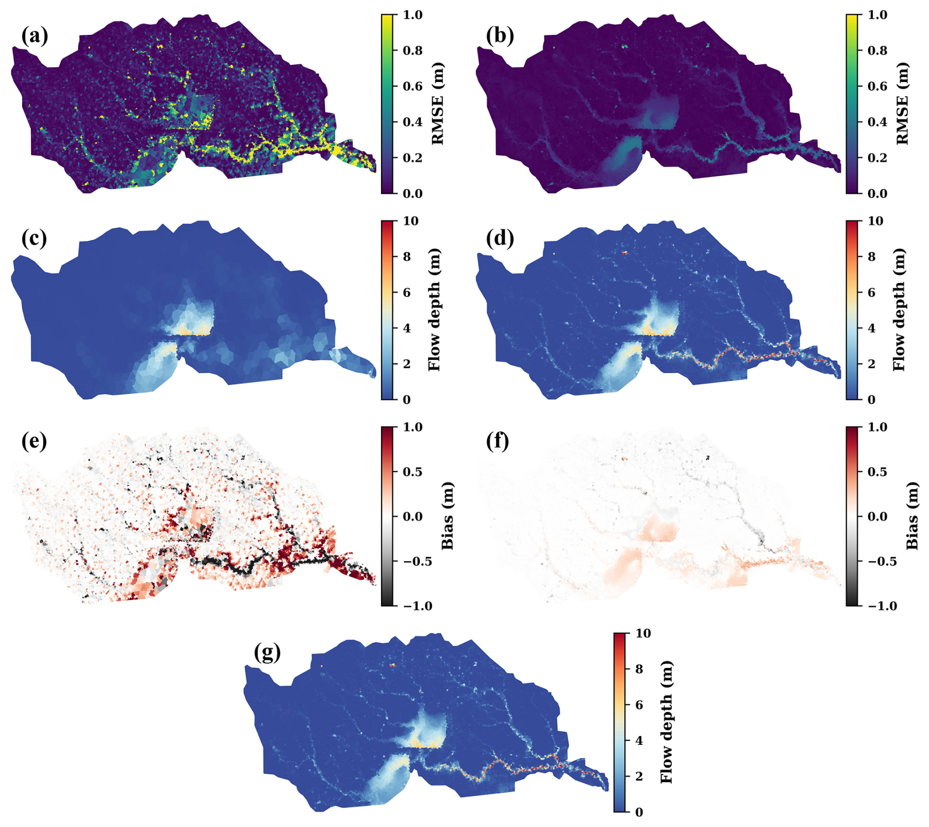
Figure 4 Root mean square error (RMSE) of the LF simulated (a) and downscaled flow depth (b) for the entire PGW event, the LF simulated (c) and downscaled flow depth (d) at 01:00 CST on 27 August (the peak flood time), the bias of the LF simulated (e) and downscaled flow depth (f) at the peak flood time, and the HF simulated flow depth (g) at the peak flood time. RMSE and bias are calculated by treating the HF simulation as “ground truth”.

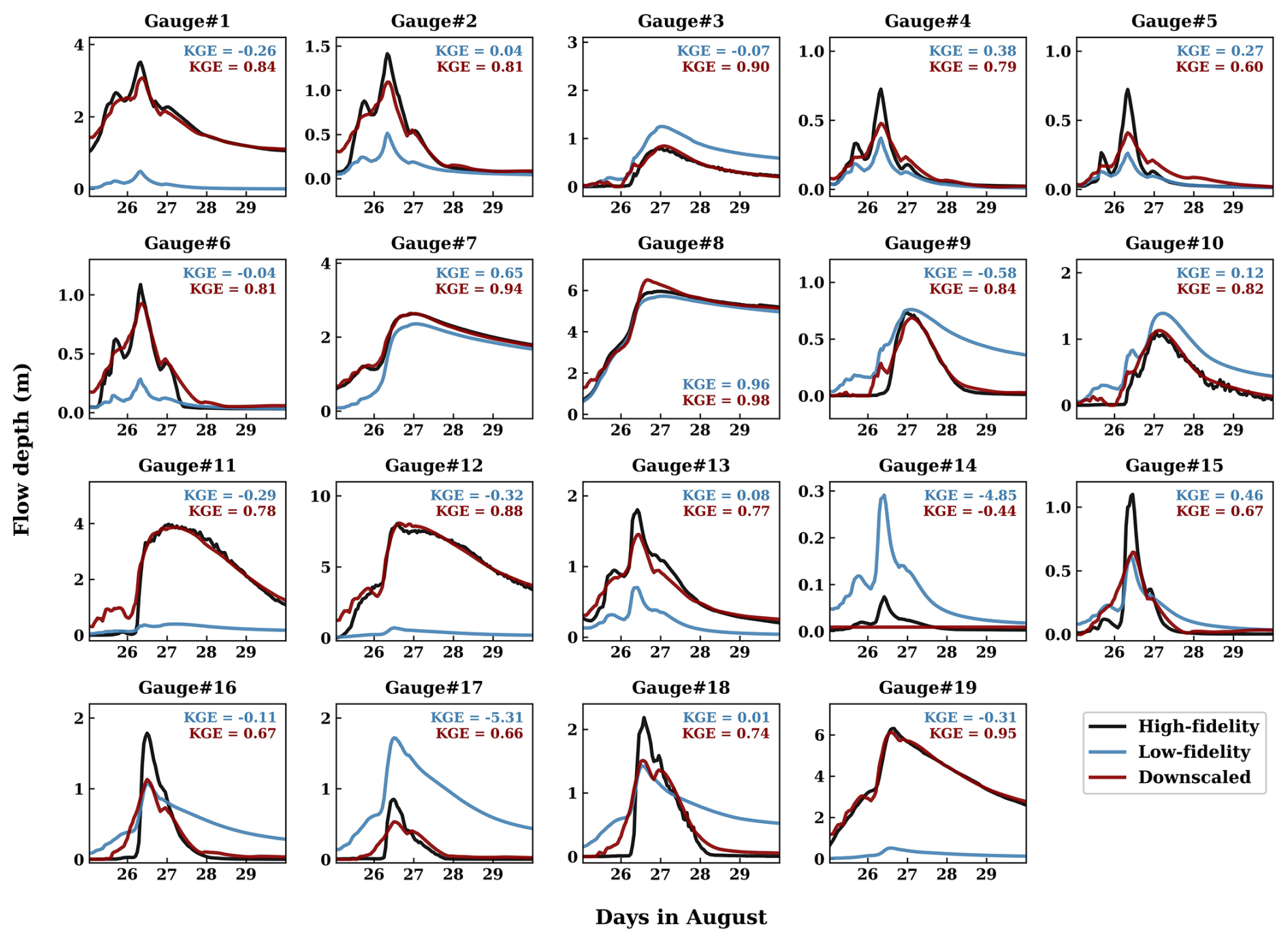
Figure 5 Comparison of the HF simulated, LF simulated, and downscaled flow depth at the selected USGS gauges during the PGW event.

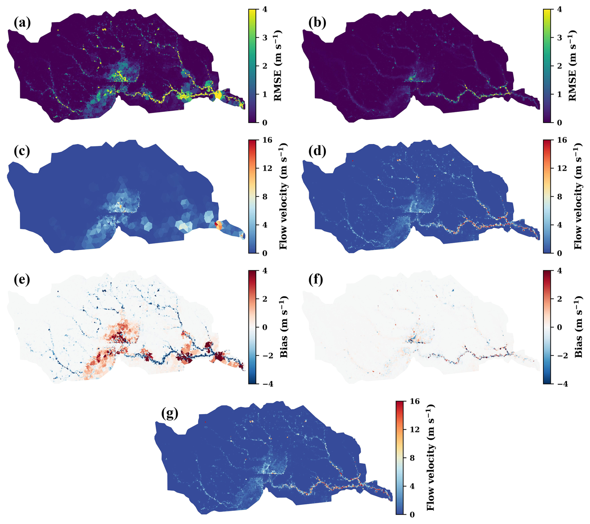
Figure 6 RMSE of the LF simulated (a) and downscaled flow velocity (b) for the entire PGW event, the LF simulated (c) and downscaled flow velocity (d) at 01:00 CST on 27 August (the peak flood time), the bias of the LF simulated (e) and downscaled flow velocity (f) at the peak flood time, and the HF simulated flow velocity (g) at the peak flood time. RMSE and bias are calculated by treating the HF simulation as “ground truth”.

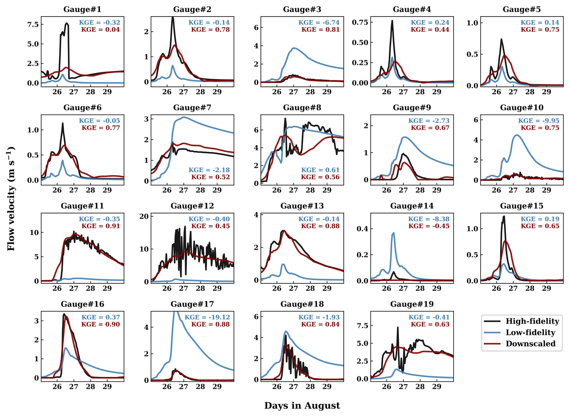
Figure 7 Comparison of the HF simulated, LF simulated, and downscaled flow velocity at the selected USGS gauges during the PGW event.

3 Results

3.1 Validation of downscaled flow depth

The trained LSG models can accurately predict the spatial and temporal variabilities of flow depth (Figs. 4 and 5) and velocity (Figs. 6 and 7) for the PGW flood event. First, the results confirm the effectiveness of the EOF analysis in extracting the significant spatial and temporal modes of the 2-D shallow water equations (Figs. S4 and S5 in the Supplement). Notably, as indicated by the proportion of variance explained by the specific modes, the significant modes of flow velocity (Fig. S5) are less representative of its variability compared to those of flow depth (Fig. S4), likely due to the higher nonlinearity of flow velocity simulations. Second, the trained LSG models perform remarkably well in reconstructing the HF ECs of river hydrodynamics from the LF ECs for both the training (Figs. S6 and S7 in the Supplement) and prediction phases (Figs. S8 and S9 in the Supplement). This performance is achieved despite substantial distinctions between the HF and LF ECs. Consequently, the spatial and temporal features of the high-resolution flow depth and velocity are well reproduced for both the training (Figs. S10–S13 in the Supplement) and prediction phases (Figs. 4–7), even though they are forced by two distinct hurricane events (Fig. 3).

During the PGW flood, using the HF simulation as the reference, the average RMSE of the downscaled flow depth is 0.07 ± 0.1 m (Fig. 4b), which is less than one-fourth of the average RMSE (0.3 ± 0.6 m) of the simulated LF flow depth (Fig. 4a). The downscaling achieves impressive error reductions in river channels (particularly downstream reaches), the nearby floodplains, and the two reservoirs (Fig. 4), which are flood-prone areas that have been deliberately refined in the high-resolution mesh (Fig. 2c). By downscaling, the detailed longitudinal variations of flow depth in the HF simulation (Fig. 4g) are precisely reproduced (Fig. 4d) during the peak flood period (near 01:00 CST, 27 August). Even very small ponding grid cells, which are barely seen in the LF simulation (Fig. 4c), are recovered (Fig. 4d). Compared to the LF simulation, the downscaled flow depth is highly consistent with the HF simulation at the peak flood time, with the bias range (from the 10th percentile to the 90th percentile) reduced from [−0.2 m, 0.3 m] (Fig. 4e) to [−0.04 m, 0.06 m] (Fig. 4f). Generally, the downscaling reduces the underestimation and overestimation of the LF simulated flow depth in river channels and floodplains, respectively, likely due to the use of the HF EOFs (Fig. S4).

The downscaling approach also performs promisingly in reproducing the temporal variability of the HF simulated flow depth at the selected USGS gauges (Fig. 5). The downscaled flow depth achieves KGE ≥ 0.5 (good performance) at all gauges except Gauge #14, where a small inundation occurs. In contrast, the LF simulation only achieves KGE ≥ 0.5 at two gauges but exhibits poor performance (KGE < −0.41; Knoben et al., 2019) at three gauges, whereas the performance at the other gauges is barely acceptable (−0.41 < KGE < 0.5). Notably, for four gauges (#3, #7, #8, and #19), the downscaling approach achieves KGE ≥ 0.9 (excellent performance). Not only does the downscaling reduce the severe biases of the LF simulation at nearly all gauges, but it also recovers dynamics not captured by the LF simulation, such as the second peak flow depth at Gauge #18.

3.2 Validation and enhancement of downscaled flow velocity

Likewise, the downscaled simulations provide accurate representations of the spatial and temporal variabilities of flow velocity during the PGW flood (Figs. 6 and 7). The downscaling significantly reduces the average RMSE of simulated flow velocity from 0.7 ± 1.9 m s⁻¹ (Fig. 6a) to 0.2 ± 0.6 m s⁻¹ (Fig. 6b). Compared to flow depth, the error reduction in flow velocity is more concentrated in the river channels, possibly reflecting the larger gradients of flow velocity from river channels to the nearby floodplains. Like flow depth, the downscaling successfully recovers the detailed longitudinal variations of flow velocity in the HF simulation (Fig. 6g), as well as the river flow in small inundated areas during the peak flood period (Fig. 6d). The method also yields substantial reductions in the estimation bias at the peak flood time, from [−0.4 m s⁻¹, 0.3 m s⁻¹] (Fig. 6e) to [−0.07 m s⁻¹, 0.05 m s⁻¹] (Fig. 6f).

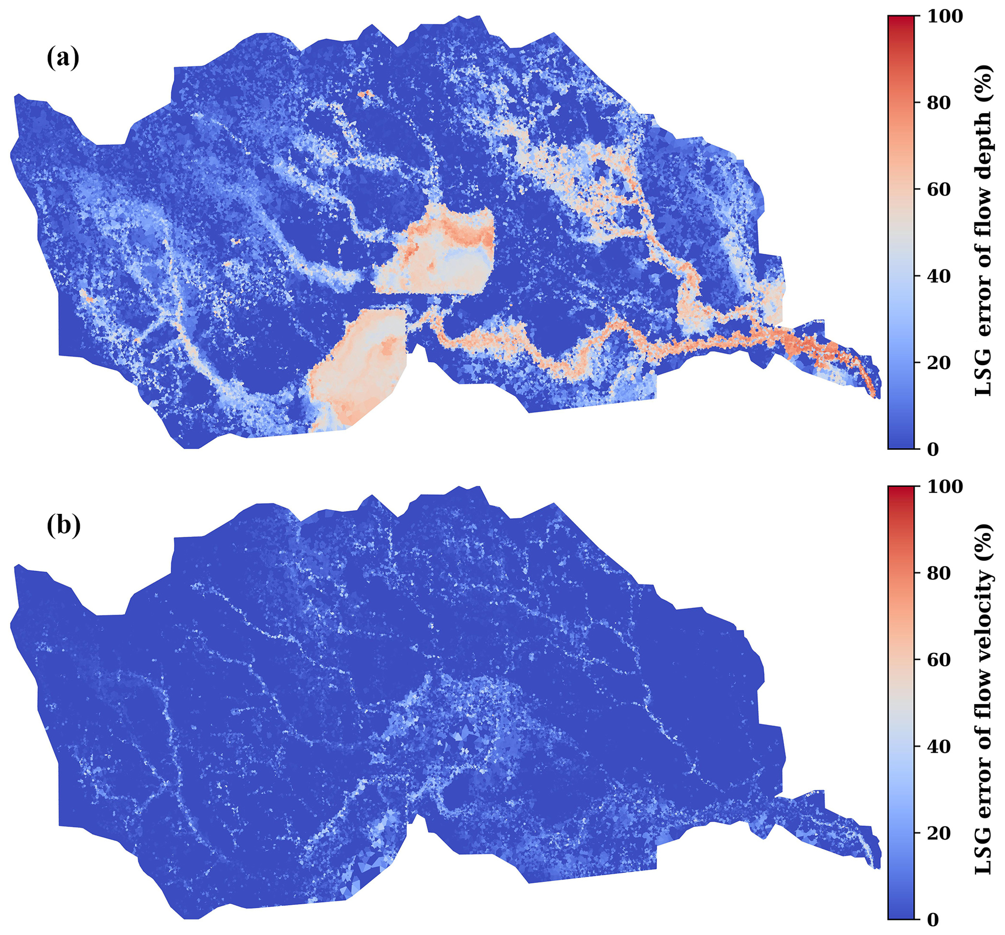
Figure 8 Percentage of flow depth (a) and velocity (b) downscaling uncertainty that can be explained by the error from the LSG model.

The downscaling also produces more consistent temporal variability of flow velocity compared with the HF simulation at the selected USGS gauges (Fig. 7). The downscaled flow velocity achieves KGE ≥ 0.5 (good performance) at 15 gauges and KGE ≥ 0.9 (excellent performance) at two gauges (#11 and #16). In contrast, the LF simulation only achieves KGE ≥ 0.5 at Gauge #8 but exhibits unacceptable performance (KGE < −0.41) at nine gauges. However, despite its superiority to the LF simulation, the downscaled flow velocity does not perform as well as the downscaled flow depth at many of the study gauges. For instance, it fails to capture the velocity spike at Gauge #1 and greatly underestimates the velocity peaks at several other gauges (e.g., #2, #4, and #8). The downscaled solutions also struggle to reproduce the high-frequency fluctuations of flow velocity, such as at Gauges #12 and #18. Analysis of the error sources indicates that for the downscaled flow velocity, the error from dimensionality reduction ER_DR is substantially larger than the LSG model error ER_LSG, while for the downscaled flow depth, ER_LSG is dominant (Fig. 8). First, this result aligns with the EOF analysis (Fig. S5), which shows the higher nonlinearity of flow velocity simulations. Second, this implies that reducing ER_DR is crucial for more accurate flow velocity downscaling.

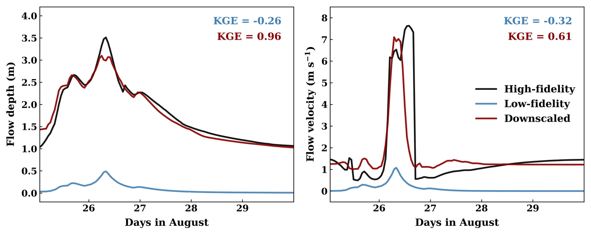
Figure 9 Comparison of the HF simulated, LF simulated, and downscaled flow depth and velocity at Gauge #1 during the PGW event when training LSG models in a focused area around the gauge (Fig. S14).

A possible way to reduce ER_DR is to regionalize the training of the LSG model in a smaller domain that focuses on a specific geographic feature. This approach can prevent locally important EC modes from being filtered out in large-scale EOF analyses (see Fraehr et al., 2023a, for North's test and Kaiser's rule). Notably, this treatment does not require new model simulations and follows the same procedure outlined in Fig. 1. We selected Gauge #1, where the whole-domain downscaling fails to reproduce the peak flow velocity simulated by the HF model. By training a new LSG model over a smaller area encompassing the gauge (Fig. S14 in the Supplement), the downscaled simulation aligns with the HF model for predicting the flow velocity spike on 26 August (Fig. 9). For the PGW event, the KGE for the simulated flow velocity increases significantly from 0.04 to 0.61. The regionalized training also slightly improves the accuracy of the downscaled flow depth at Gauge #1, with KGE increasing from 0.81 to 0.96. The smaller effect of regionalized training on flow depth is expected because our error analysis indicates that the uncertainty of the downscaled flow depth is only minorly contributed by ER_DR (Fig. 8).

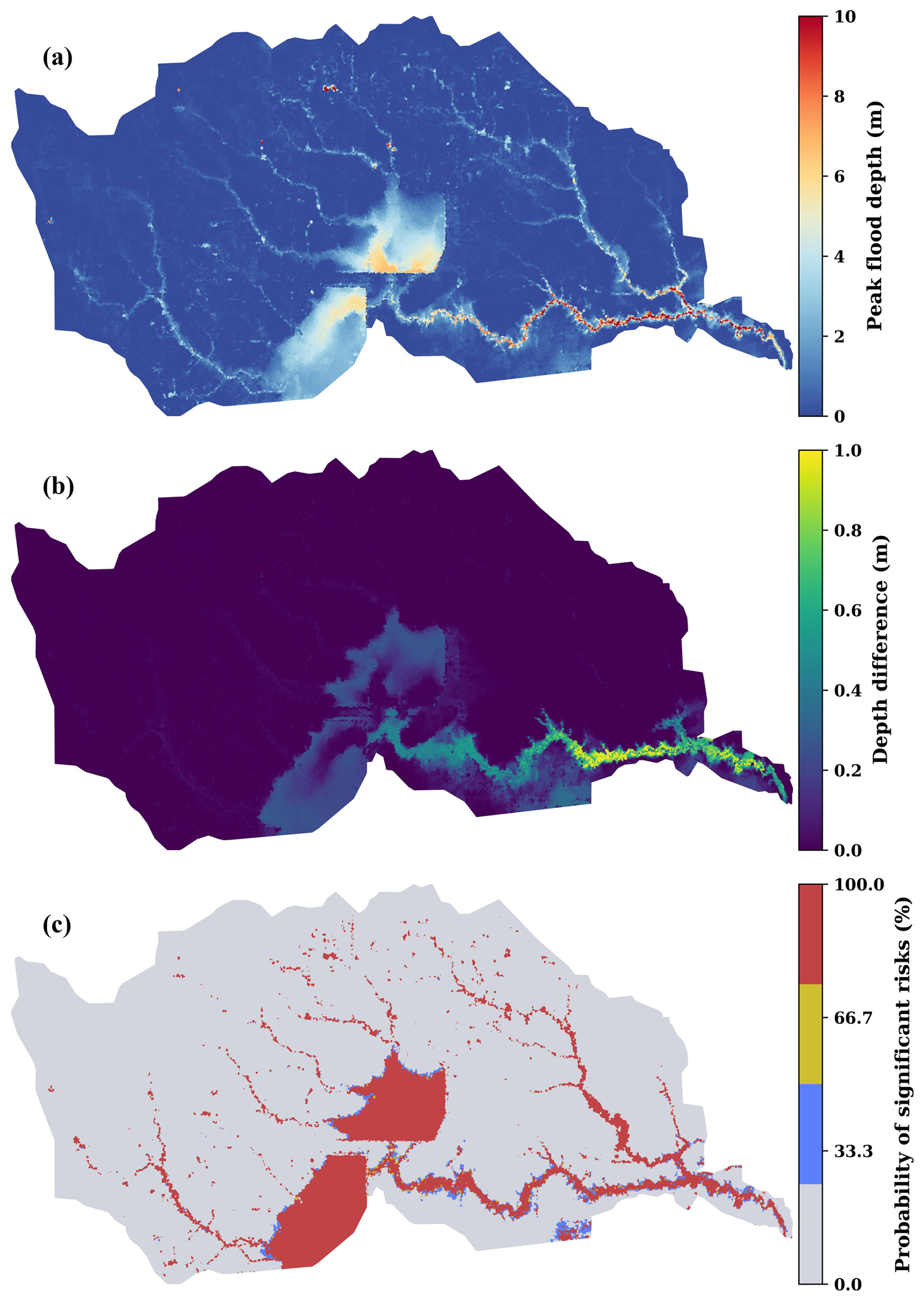
Figure 10 Projected peak flood depth of the PGW ensemble simulation (a), the difference of the projected peak flood depth between the PGW ensemble simulation and the selected PGW simulation (b), and the probability of significant risks to human safety from flooding (c).

3.3 Ensemble inundation downscaling

Because the training of the LSG model can be completed within minutes, the computational cost of our downscaling approach depends solely on the computational time needed for the RHM simulations. For the 13 d PGW simulations, when running on Intel Xeon Skylake CPUs (2.4 GHz) with 192 GB of DDR4 DRAM, the HF model (664 724 grid cells) requires 4032 CPU hours to complete, while the LF model (14 536 grid cells) requires only 48 CPU hours. Thus, by applying the downscaling approach to the LF ensemble simulations, our method provides an efficient way to evaluate the impact of the uncertainty in tropical cyclone (TC) predictions on the simulation of urban flooding. Figure 10 shows that compared to the single-member PGW simulation described in the above evaluation, a three-member ensemble of PGW simulations predicts higher peak inundation depths in the lower reaches of the Buffalo Bayou watershed, where population density is also the highest. In some areas, the difference in peak flood depth during the PGW event can exceed 1 m (Fig. 10b). Using the ensemble simulations, we can also calculate the likelihood of the areas where the PGW flood event poses significant or high risks to human safety (h > 0.95 m; Russo et al., 2013). From the ensemble simulations, humans will very likely face significant risks from floodwater in the two reservoirs, river channels, and the nearby areas in Houston during the PGW flood event (Fig. 10c). In line with Fig. (10b), some simulations predict larger extents of the areas where the flood event would pose significant risks to human safety.

4 Discussion

4.1 Simulation of high-resolution river hydrodynamics

Our results demonstrate that the LSG-model-based downscaling approach can provide efficient and accurate simulations of high-resolution river hydrodynamics at the computational cost of LF RHMs. To the best of our knowledge, this is one of the first studies to explore methods for fast and accurate simulations of high-resolution flow velocity in realistic cases, broadening the usefulness and relevance of recent rapid progress in hydrodynamic modeling, which still exclusively focuses on flooding (Carreau and Guinot, 2021; Xie et al., 2021; Zhou et al., 2021; Feng et al., 2023b; Fraehr et al., 2023b; Frame et al., 2024; Wing et al., 2024). With HF simulations of flow velocity, our understanding of not only instantaneous flood hazards but also longer-timescale environmental hazards, such as eutrophication and pollution, can be greatly advanced. More broadly, the new method can contribute to the development of fully coupled atmosphere–land–river–ocean ESMs, which will be discussed in detail in Sect. 4.2. It is worth noting that the study watersheds of Fraehr et al. (2023a, 2023b) differ from this study in land use and climate. The two Australian watersheds in Fraehr et al. (2023a, 2023b) are dominated by rural and natural landscapes and are less affected by TCs. The success of the LSG model in different domains underscores its broad geographical applicability.

The LSG-model-based downscaling approach has two major advantages over neural network (NN)-based methods for high-resolution river hydrodynamic modeling. First, compared to NN-based methods (Tran et al., 2023), the training time of the LSG method is negligible, requiring only one expensive HF RHM simulation for training. Second, because physical laws have been explicitly coded in LF RHMs and implicitly complied with in the spatial interpolation process, the trained model can be expected to be transferable to future unseen climate conditions. These advantages make the approach well-suited for ensemble projections of future flooding, which are crucial for robust assessment of flood adaptation and mitigation (Fig. 10) given the substantial uncertainty of TC projections (Fig. 3). Another potential strength of our approach is that it can directly benefit from future advances in RHMs. The development of better RHMs will provide more accurate LF and HF simulations of river hydrodynamics for LSG model training, helping to reduce downscaling uncertainty (Fraehr et al., 2023a).

While a well-trained LSG model can be applied to unseen climate conditions, it is not free from retraining. For instance, without retraining, an LSG model is unlikely to handle changes in land use and geographical features, such as geomorphological changes in river channels and river flow modifications related to reservoirs. Additionally, our training strategy, which trains the LSG model only with data from the Harvey flood event, may not be effective in more complex cases where floods are not always driven by TCs. For instance, the main flood mechanisms in the US Mid-Atlantic watersheds include both rain-on-snow (ROS) and snowmelt events that mainly occur in high-latitude areas (e.g., 1996 ROS flood) and heavy rainfall from tropical cyclones (e.g., Hurricane Irene in 2011), extratropical systems, and convective systems (Smith et al., 2010; Li et al., 2021; Sun et al., 2024). For such cases, it is necessary to follow the training procedure of Fraehr et al. (2023a), selecting multiple representative flood events of different types for training. Since the number of flood mechanisms is limited, we expect that the computational demand will still be manageable even if the LSG model is applied to a watershed with diverse flood generation processes.

Our study reveals that the downscaling accuracy of flow velocity is lower than that of flow depth. This is because the dynamics of flow velocity are more nonlinear, which induces significantly larger dimensionality-reduction errors in the downscaling process (Fig. 8). Accordingly, we introduced a regionalized training procedure to improve the downscaled flow velocity in focused areas (Fig. 9). This procedure does not significantly increase the computational cost of the LSG model because it does not require any new RHM runs. We envision that this strategy can be particularly useful for simulating river hydrodynamics in geographical areas that need more careful flood risk assessments, such as schools, hospitals, critical infrastructures, energy facilities, and Superfund sites (Brand et al., 2018).

The LSG model error ER_LSG primarily depends on the performance of the sparse GP model in mapping LF ECs to HF ECs. Besides the sparse GP model, other data-driven models, such as multilayer perceptrons and artificial neural networks, can also be used to establish the complex relationships between ECs (Carreau and Guinot, 2021). Future research on implementing other data-driven models to reduce ER_LSG is also worth exploring.

The LF model used in this study is about 84 times faster than the HF model, which is significantly more efficient than the LF model adopted by Fraehr et al. (2023a) that is only 12 times faster. Also, our LF model achieves a larger acceleration rate than the theoretical boost rate when considering the reduction in the number of grid cells ($\frac{\mathrm{664}\mathrm{724}}{\mathrm{14}\mathrm{536}}\approx \mathrm{46})$. The improved efficiency indicates that the OFM RHM has taken advantage of fewer computational units and longer time steps according to the Courant–Friedrichs–Lewy convergence criteria in the simulations. Furthermore, the results underscore the usefulness of our approach for flood risk assessment, which needs hundreds or thousands of ensemble model runs for uncertainty quantification (Wu et al., 2020), which the configuration of Fraehr et al. (2023a) cannot provide due to its inefficient LF simulations.

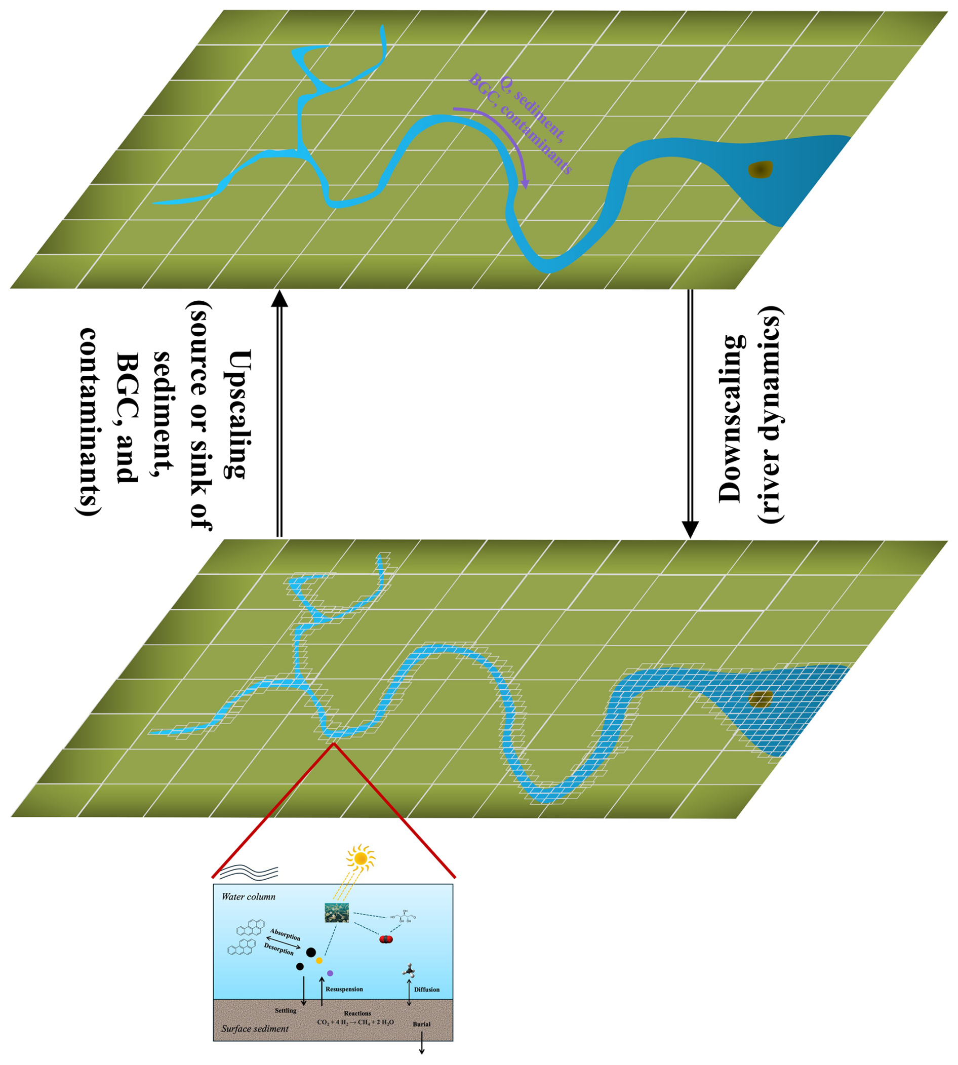
Figure 11 A schematic illustration of coupling large-scale hydrodynamical processes that are simulated in coarse resolution with local physical, chemical, and biological processes that are simulated in fine resolution in river models.

4.2 Coupling large-scale hydrodynamical processes with local processes in river models

It is challenging to represent other physical, chemical, and biological processes beyond river discharge in large-scale river models. This is mainly because, by sacrificing process and resolution accuracy for computational efficiency, these models cannot provide accurate simulations of high-resolution flow depth and velocity necessary for calculating local dynamics important for fluvial processes (Bertagni et al., 2024), such as sediment settling velocity (Li et al., 2022), bottom shear stress and diffusivity (Chen et al., 2023), and greenhouse gas outgassing velocity (Ulseth et al., 2019). By accurately and efficiently simulating high-resolution flow depth and velocity, our downscaling approach provides an opportunity to bridge the gaps between large-scale hydrodynamical processes and detailed local processes in river models. Specifically, we propose a two-way coupling scheme in large-scale river models (Fig. 11). In the first stage of each simulation cycle, a large-scale river model is used to simulate coarse-resolution flow depth and velocity and transport mass and momentum downstream. In the second stage, the LSG-model-based approach is employed to downscale the simulated flow depth and velocity to fine resolutions. In the third stage, high-resolution hydrodynamics are used to drive detailed physical, chemical, and biological models, such as the PFLOTRAN model for geochemistry (Hammond et al., 2012) and the GAIA model for sediment (Tassi et al., 2023), to simulate the sources and sinks of the represented tracers. In the final stage, the sources and sinks calculated in the fine-resolution mesh are upscaled to the coarse-resolution mesh of the large-scale river model and used to update the concentrations of the represented tracers.

An outstanding weakness of existing ESMs is that they ignore the lateral biogeochemical fluxes in the land–river–ocean continuum and therefore do not close the global biogeochemical cycles (Regnier et al., 2022). By implementing this new paradigm of river modeling in ESMs, land, river, and ocean biogeochemistry will be fully coupled, helping to close the global biogeochemical cycles. To achieve this vision, future research must focus on extending the LSG-model-based approach to downscale 1-D river models to 2-D fine-resolution meshes. This is because, despite the prospect of 2-D large-scale river models running on GPU-based supercomputers, 1-D river models will likely still be the default configuration in ESMs in the near future (Telteu et al., 2021). We envision that the potential challenges could include the alignment of 1-D and 2-D unstructured meshes and the interpolation of simulated 1-D river hydrodynamics onto 2-D meshes.

5 Conclusion

In this study, we developed a downscaling approach based on the LSG model to achieve fast and accurate simulations of high-resolution river flow depth and velocity. Our test of TC-induced flood events in an urban watershed in Houston demonstrates the effectiveness and efficiency of the downscaling method, as the simulation errors in the LF RHM are greatly reduced, without additional computational costs. We further indicated that the simulation error of the downscaled flow velocity can be reduced by employing regionalized training of the LSG model for selected focus areas. As one of the first studies to explore high-fidelity and efficient flow velocity simulations in realistic cases, our research can help broaden the usefulness and relevance of the recent rapid progress in hydrodynamic modeling, which still exclusively focuses on flooding. More importantly, the downscaling approach provides an opportunity to bridge the gaps between large-scale hydrodynamical processes and local physical, chemical, and biological processes in river models, which could eventually help close the global biogeochemical cycles in ESMs.