Will rivers become more intermittent in France? Learning from an extended set of hydrological projections

This study aims to assess the changes in the intermittence of river flows across France in the context of climate change. Projections of flow intermittence are derived from the results of the Explore2 project, which is the latest national study that proposes a wide range of potential hydrological futures for the 21st century. The multi-model approach developed within the Explore2 project enables uncertainties in future flow intermittence to be characterized. Combined with discrete observations of flow states, hydrological projections are post-processed to compute the daily probability of flow intermittence (PFI) on each element of the partition of France in hydro-ecoregions (HERs).

The post-processing consists of calibrating logistic regressions between the historical flow states of the National Low-Flow Observatory (ONDE) network and the flow data simulated by the hydrological models involved in Explore2 run with the SAFRAN atmospheric reanalysis as inputs. After calibration, these regressions are used to project daily PFIs for the entire 21st century, based on flow simulations from five hydrological models driven by up to 17 climate projections under RCP2.6, RCP4.5, and RCP8.5 climate change scenarios.

The results show good agreement among the hydrological models regarding the increase in flow intermittence under RCP4.5 and RCP8.5. The projected increase in mean daily PFI between July and October and the shift of the first and last days when PFI exceeds 20 % both suggest a gradual intensification and extension of dry spells throughout the century. The southern regions of France are likely to experience greater increases in runoff intermittence than the northern regions, and mountainous regions such as the Alps and the Pyrenees are likely to experience changes in their dynamics of intermittence with a reduction in winter intermittence and the apparition of or increase in summer intermittence. The uncertainty of these projected changes is larger in northern France due to greater intermodel variability in this region.

1 Introduction

Intermittent rivers and ephemeral streams (IRESs) are watercourses characterized by the absence of continuous year-round water flow (Sefton et al., 2019). While water management practices can exacerbate flow intermittence by altering runoff patterns, climatic factors – particularly aridity – remain the primary determinants of these systems (Addor et al., 2018; Hammond and Fleming, 2021; Sauquet et al., 2021; Zipper et al., 2021). In recent decades, climate change has intensified these dynamics, significantly impacting the global water cycle: summer precipitations tend to decrease, and rising temperatures have increased evapotranspiration and driven more frequent heatwaves (Douville et al., 2021). These changes have led to more severe low-flow periods and more frequent and widespread dry spells in Western Europe (Delso et al., 2017; Tramblay et al., 2020; Vicente-Serrano et al., 2020). Meanwhile, IRESs play a critical role as interfaces between terrestrial and aquatic ecosystems. Altered patterns of flow interruption can therefore compromise water quantity and quality in downstream perennial rivers, increase extinction risks for specialized species, and disrupt organic matter, nutrient, and sediment cycles (Bertassello et al., 2022; Gallart et al., 2012; Giezendanner et al., 2021; Finn et al., 2011; Meyer et al., 2007; Sarremejane et al., 2017; Larned et al., 2010). Hence, a better understanding of IRES behaviours and their interaction with perennial streams is needed to assess the impacts of ongoing and future changes on river ecosystems (Döll and Schmied, 2012; Jaeger et al., 2014; Pumo et al., 2016; Leigh and Datry, 2017) and to address water management challenges (Acuña et al., 2014).

Globally, IRESs account for nearly two-thirds of river networks (Schneider et al., 2017; Messager et al., 2021), with this proportion reaching 39 % in France (Snelder et al., 2013). Their spatial and temporal dynamics can be characterized using conceptual models of network contraction (Shaw et al., 2017; Botter and Durighetto, 2020) or through semi-conceptual and machine learning frameworks that integrate hydroclimatic and physiographic factors (Lapides et al., 2021; Durighetto et al., 2022). The strongest predictors of flow intermittence are aridity indices (Vicente-Serrano et al., 2019; Jaeger et al., 2019). However, local variations in permeability, lithology, and topography also influence intermittence patterns in specific regions, including West Africa (Yu and Duffy, 2018; Belemtougri et al., 2021), northern Spain (González-Ferreras and Barquín, 2017), and northwestern Australia (Bourke et al., 2021). Studying intermittence at a large scale therefore requires considering the diversity of hydrological processes at play, particularly when multiple watersheds exhibit diverse sensitivities to hydroclimatic conditions. This variability highlights the need for robust methodologies to assess intermittence at national to (semi-)continental scales (Addor et al., 2018; Hammond and Fleming, 2021; Sando et al., 2022; Döll et al., 2024).

Understanding the drivers of river intermittence is also crucial for analysing historical trends and projecting future changes in IRES behaviour. Climate change has already expanded the spatial and temporal extent of intermittent flows worldwide (Zipper et al., 2021; Jaeger et al., 2019; Sando et al., 2022; Gudmundsson et al., 2021), and the Mediterranean basin is particularly affected (Tramblay et al., 2020; De Girolamo et al., 2022). However, interpreting climate projections and emission scenarios at the scale of headwater basins remains rare (Schneider et al., 2013). Indeed, many climate models have a coarse spatial resolution, and high uncertainties emerge from multi-model ensembles (MMEs), which makes accurate predictions of future IRES changes difficult.

To address these challenges, France has implemented the Explore2 project (https://entrepot.recherche.data.gouv.fr/dataverse/explore2-projections_hydrologiques, Sauquet et al., 2025b) that uses a multi-model, multi-scenario approach to simulate hydrological conditions throughout for the 21st century. It assesses uncertainties at each step of the modelling process. However, the resolution of the climate projections involved in Explore2 is too coarse to accurately capture IRES dynamics. Hence, this study extends the results of Explore2 for purposes of generating flow intermittence projections for French headwater streams. To this end, we follow a statistical approach that estimates the daily probability of flow intermittence (PFI) in small streams based on streamflow data simulated by Explore2 for larger perennial rivers. The estimated PFI serves as a proxy indicator for the intensity and duration of dry periods. The method is calibrated using field observations carried out regularly at more than 3200 upstream river sites prone to drying.

To achieve this, the present work builds on two key studies: Beaufort et al. (2018), which demonstrated consistent performance of PFI estimation across the heterogeneous climate of France using daily discharge, and Sauquet et al. (2021), which projected PFI under a limited set of climate projections with coarse spatial resolution. In contrast, this study incorporates a finer spatial resolution, a broader range of climate scenarios, and a wider variety of hydrological models thanks to the integration of Explore2 projections. It therefore addresses a critical research gap by generating projections of small-stream intermittence across France and throughout the 21st century while quantifying the associated uncertainties.

The remainder of the paper is organized into five sections. The data used are outlined in the second section. Section 3 describes the statistical method linking PFI to hydrological projections. Section 4 presents the results, which focus on the mean daily PFI between July and October (mPFI_7–10) and the median of the first and last days (respectively, Tf and Tl) when PFI exceeds 20 %. Finally, Sect. 5 discusses these results, and Sect. 6 concludes the study.

2 Data

2.1 Monitoring river flow intermittence

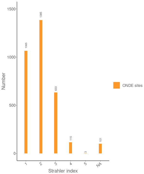
The French Biodiversity Office (OFB; https://ofb.gouv.fr/, last access: 18 August 2024) initiated in 2012 the National Low-Flow Observatory (ONDE) to gain a better understanding of low flows and intermittent rivers. ONDE is a stream intermittence monitoring network comprising 3248 observation sites strategically distributed across the French river network with the aim of characterizing the occurrence and the intensity of summer (low-)flows. The network has been designed to focus on streams with a Strahler order ranging from 1 to 4, which are prone to natural and/or anthropogenic intermittent flow conditions. Most sites (85 %) are located on “small streams” with a drainage area ≤100 km², 75 % are situated on streams with a Strahler index of 1 or 2, and 20 % of the sites have a drainage area ≤10 km² (Appendix Figs. G1 and G3).

A key feature of the ONDE network is that it involves the flow state of watercourses, which results from the visual inspection of streams by OFB observers at each location instead of a sensor-based measurement of flow rates. In the present study, two binary categories are defined for ONDE observations: (1) “visible flows” and (2) “dry conditions”, which gather non-visible flows (standing water in isolated pools) and totally dry conditions (dry riverbed at or near the ONDE site). We use only data from regular and structured field campaigns (referred to as “usual campaigns” in the ONDE nomenclature), during which the ONDE sites are monitored systematically in mainland France around the 25th day of each month from May to September. Here we use ONDE data from 2012 to 2022 for model calibration and evaluation.

Based on ONDE data, the PFI is defined as the proportion of small streams under drying conditions at the regional scale. It is used as a proxy indicator for the intensity and duration of dry periods. Long-term analysis of the PFI characterizes the spatial and temporal trends of drought across regions and provides valuable information about IRES intermittent behaviour.

2.2 Delineating areas with homogeneous hydrological behaviour: the hydro-ecoregions

Hydro-ecoregions (HERs) are spatially homogeneous areas defined over France based on natural drivers involved in river ecosystem functioning, such as geology, topography, and climate. There are 85 level-2 HERs (HER2s) across France, and they are derived from the sub-division of 22 level-1 HERs (HER1s) (Wasson et al., 2002), which were used in a previous study about the impact of climate change on PFI in France (Sauquet et al., 2021). In contrast, the present study investigates flow intermittence at the scale of HER2s in order to model PFI at a higher spatial resolution. The statistical approach developed hereafter requires sufficient observations of flow states for calibration purposes (see Sect. 3.1), which led us to perform five groupings of HER2 in order to ensure that enough observations are available for model calibration. When merging HER2s we checked that they belonged to the same level-1 HERs to ensure that they share similar environmental characteristics at the large scale. In the end, a partition of France into 75 entities (HER2 or pool of HER2s) was considered for this study (Fig. 1).

These 75 HER2s have a median surface area of 4990 km², and more than 20 % ($\mathrm{17}/\mathrm{75}$) have a surface area greater than 10 000 km². The HER2s were the subject of ONDE field campaigns from May to September between 2012 and 2022, thus resulting in 4125 campaigns. A total of 78 campaigns are excluded from the analysis due to their failure to cover more than 75 % of the monitoring stations within a given HER2. Thus, the data exclusion rate from the ONDE network is less than 2 %, leaving 4047 field campaigns with usable data.

Figure 1 Delineation of level-2 hydro-ecoregions (HER2s) across France. The four HER2s that are used for illustration in this study are highlighted in purple (see Sect. 3.7).

2.3 Future hydrological projections over France: the Explore2 project

The assessment of changes in the PFI over the 21st century is based on the large set of hydrological projections produced by the Explore2 project (Sauquet et al., 2025a). The daily discharge projections were obtained at about 4000 simulation points distributed along the French river network, with a constraint on the minimum drainage area imposed by the spatial resolution of climate projections (64 km²) and another constraint of an even coverage across France.

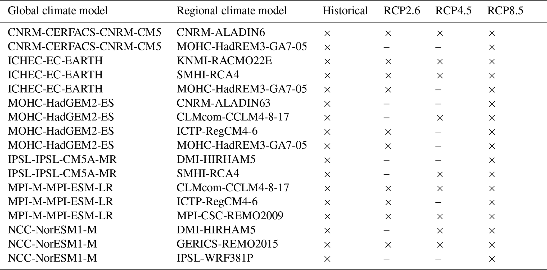
Explore2 is a multi-model simulation experiment involving nine different hydrological models, but some of them are restricted to regional applications (on average each simulation point has discharge projections simulated by four hydrological models). Finally, with the objective of predicting flow intermittence at the national scale, we select the five models with the largest simulation domain: CTRIP (Decharme et al., 2019), GRSD (de Lavenne et al., 2016), J2000 (Morel et al., 2023), ORCHIDEE (Huang et al., 2024), and SMASH (Jay-Allemand et al., 2020). The Explore2 project considers only natural flows, although some of the hydrological models involved in the project have the capability of including human-induced influences. The evaluation of hydrological models was performed using an extended dataset of near-pristine catchments (Strohmenger et al., 2023). The simulations used for model evaluation were carried out for the period 1976–2022 using the French near-surface SAFRAN meteorological reanalysis (Vidal et al., 2010) as input. In addition, the hydrological models included in Explore2 have been evaluated on the common period of availability 1976–2019 (Sauquet et al., 2025a). After validation, the hydrological models are forced by an ensemble dataset derived from 17 pairs of global and regional climate models (GCM–RCM) corrected by the statistical adjustment method ADAMONT (Verfaillie et al., 2018) for both historical (1976–2004) and future climate scenarios RCP2.6, RCP4.5, and RCP8.5 (2005–2100; Appendix A). In the end, these bias-corrected climate projections were used as inputs for the hydrological models: all 17 GCM–RCM projections are used under RCP8.5 scenario, whereas 10 of these projections are used under RCP2.6 and nine under RCP4.5. The baseline period is set to 1976–2005 and used thereafter for analysing changes in IRES behaviour. Overall, the hydrological projections used thereafter to predict PFI result from combinations of RCP–GCM–RCM–hydrological models.

3 Modelling framework

3.1 Linking intermittence to stream discharge at the HER2 scale

The empirical method suggested by Beaufort et al. (2018; Eq. 4) is applied here to estimate the probability of flow intermittence (PFI) at the scale of HER2s. This method follows a two-step process that links observed flow states at ONDE sites to daily streamflows (either gauged or modelled) using logistic regressions.

First, observations from ONDE sites are used to determine the percentage of sites with “dry conditions” for each HER2 (h) and each campaign date (j). Flow intermittence evolves over relatively long timescales, with seasonal transitions between flowing and dry states occurring gradually within the year, except in cases of significant rainfall events that can temporarily trigger flow conditions. Given this inertia, the estimation of flow intermittence remains appropriate even if not all sites within a HER2 are monitored on the exact same day, with a shift of only a few days during a given campaign. To further ensure the temporal consistency across campaigns the monitoring is systematically conducted at fixed sites, and data from a given ONDE campaign and HER2 are only considered if at least 75 % of the ONDE sites within the HER2 are monitored during the campaign. This approach minimizes potential biases associated with incomplete observations, and ensures that the percentage of dry ONDE sites referred to hereafter as PFI_h(j) can be considered representative of the PFI.

Subsequently, a logistic regression model is calibrated for each HER2 in order to link the PFI values for day j to streamflow conditions (Eq. 1, Fig. 2):

$$\begin{array}{}\text{(1)}& {\mathrm{PFI}}_h\left(j\right)={\displaystyle \frac{e^{{\mathit{\beta }}_{\mathrm{0}\cdot \mathrm{HER}{\mathrm{2}}_h}+{\mathit{\beta }}_{\mathrm{1}\cdot \mathrm{HER}{\mathrm{2}}_h}\times F_{Q\cdot \mathrm{HER}{\mathrm{2}}_h}\left(j\right)}}{\mathrm{1}+e^{{\mathit{\beta }}_{\mathrm{0}\cdot \mathrm{HER}{\mathrm{2}}_h}+{\mathit{\beta }}_{\mathrm{1}\cdot \mathrm{HER}{\mathrm{2}}_h}\times F_{Q\cdot \mathrm{HER}{\mathrm{2}}_h}\left(j\right)}}},\end{array}$$

where ${\mathit{\beta }}_{\mathrm{0}\cdot \mathrm{HER}{\mathrm{2}}_h}$ and ${\mathit{\beta }}_{\mathrm{1}\cdot \mathrm{HER}{\mathrm{2}}_h}$ are, respectively, the logistic regression intercept and slope coefficient associated with the predictor $F_{Q\cdot \mathrm{HER}{\mathrm{2}}_h}$.

The model uses the mean non-exceedance frequencies of discharge $F_{Q\cdot \mathrm{HER}{\mathrm{2}}_h}\left(j\right)$ as a predictor for PFI_h(j) (Eq. 2). $F_{Q\cdot \mathrm{HER}{\mathrm{2}}_h}$ is regarded as a proxy characterizing the current wet versus dry hydrological conditions at the regional scale. It is derived from the non-exceedance frequency curves of streams, which describe the probability that a given discharge value is not exceeded. For each specific (j) corresponding to an ONDE field campaign and each HER2 (h), the daily empirical non-exceedance frequencies of discharge are spatially averaged over all available n streams whose drainage areas intersect the HER2 of interest (weighted by their drainage area) and temporally averaged over the period $[j-\mathrm{6};j]$. This 7 d window allows the inclusion of non-simultaneous response times caused by heterogeneous propagation times in the underground and the river network (the choice of a 7 d window is the result of an optimization process; see Appendix B). In the end, $F_{Q\cdot \mathrm{HER}{\mathrm{2}}_h}$ is defined by

$$\begin{array}{}\text{(2)}& F_{Q\cdot \mathrm{HER}{\mathrm{2}}_h}\left(j\right)={\displaystyle \frac{\mathrm{1}}{\mathrm{7}\times n}}{\sum }_{k=j-\mathrm{6}}^j{\sum }_{s=\mathrm{1}}^n{F}_Q(k,s),\end{array}$$

where F_Q(k,s) represents the non-exceedance frequency of each stream s among the n streams whose drainage areas intersect the HER2 h. This frequency is weighted by the drainage area of stream s. The summation is computed over each day k within the $[j-\mathrm{6};j]$ period around campaign j.

Once calibrated, the logistic regressions are used to convert the hydrological projections from the Explore2 project into PFI projections.

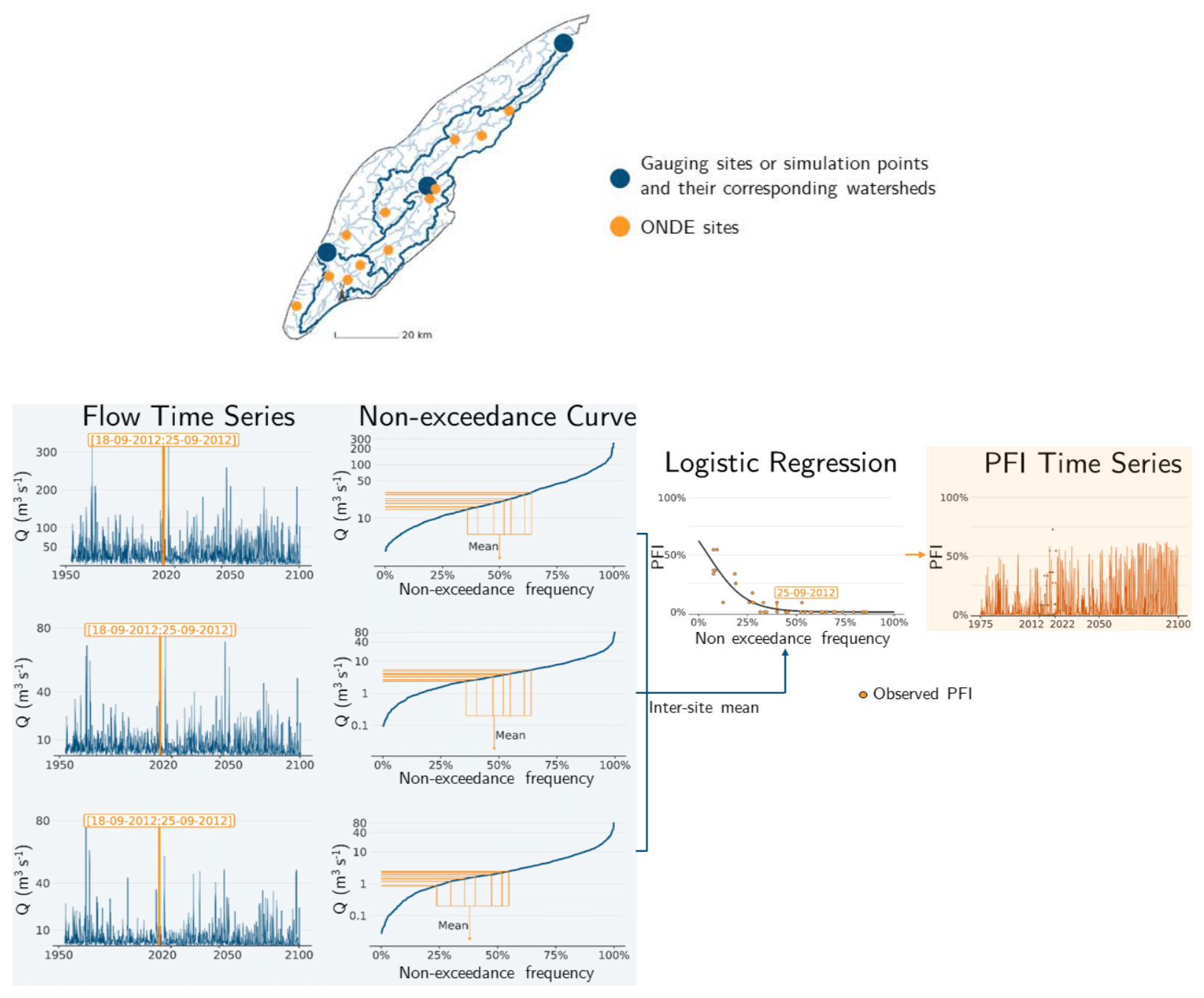
Figure 2 Schematic view of the approach adapted to derive the regional probability of flow intermittence (PFI) from ONDE sites using daily flows either gauged or modelled within a given HER2. The daily flows simulated by Explore2 at three simulation points generate flow time series (column 1) and their corresponding non-exceedance frequency curves (column 2). A logistic regression is then used to link daily flows to ONDE observations, as illustrated here for the campaign of 25 September 2012. For this campaign, daily discharge values simulated between 18 and 25 September 2012 are extracted for each simulation point whose drainage area intersects the HER2. These seven flow values are matched to their respective non-exceedance frequency using the non-exceedance frequency curve. The mean non-exceedance frequency across all simulation points is then associated with the proportion of ONDE sites exhibiting “dry conditions” during this campaign (observed PFI, column 3). The logistic regression is calibrated using data from all ONDE campaigns. Once calibrated, these models allow for the conversion of daily discharge time series into daily PFI time series for the HER2s (column 4).

3.2 Calibrating PFI logistic regression models using observed daily discharge data

Logistic regression models are preliminarily fitted between 2012 and 2022 using observed discharge data. The daily discharge data used in the calculation of $F_{Q\cdot \mathrm{HER}{\mathrm{2}}_h}$ were compiled using gauging station records from the French reference hydrologic network HydroPortail (Leleu et al., 2014) (https://www.hydro.eaufrance.fr, last access: 4 September 2023). The set of gauging stations were selected on the basis of three different criteria:

• Daily discharge data must be available during the ONDE field campaigns, i.e. within the $[j-\mathrm{10};j+\mathrm{10}]$ interval centred on the 25th of each month from May to September for the years 2012 to 2022.

• The human disturbance to flow must be minimal at the gauging stations.

• All selected gauging stations must have a drainage area of less than 2000 km². Large gauged basins with a high Strahler order have been discarded since they are unlikely to behave in the same way as small streams.

This selection process results in a final dataset including 1008 stations (Fig. 3). The non-exceedance frequency curve of each gauging station is computed using its entire available discharge time series, leading to variations in the time periods covered by the discharge data across stations. Nevertheless, limiting the analysis to the period 2012–2022 would likely exclude critical information on hydrological extremes and fail to fully capture the variability in high- and low-flow events, which are pivotal for understanding a river's behaviour during extreme conditions.

3.3 Assessing the performance of PFI logistic regression models under current climate

Several cross-validation schemes are then considered to test the robustness of these models. A leave-one-year-out cross-validation is first carried out by excluding one year at a time from the training dataset, learning from the data of the remaining years and then making estimations for the excluded year. The robustness under different climate conditions is also assessed through a differential split-sample test (DSST; Dakhlaoui et al., 2017), which is a k-fold cross-validation performed on three distinct groups of hydrological years categorized as dry, intermediate, or wet (Appendix C). The years are discriminated according to the aridity index (Barrow, 1992), which is one on the main drivers of flow intermittence at the global scale (Sauquet et al., 2021).

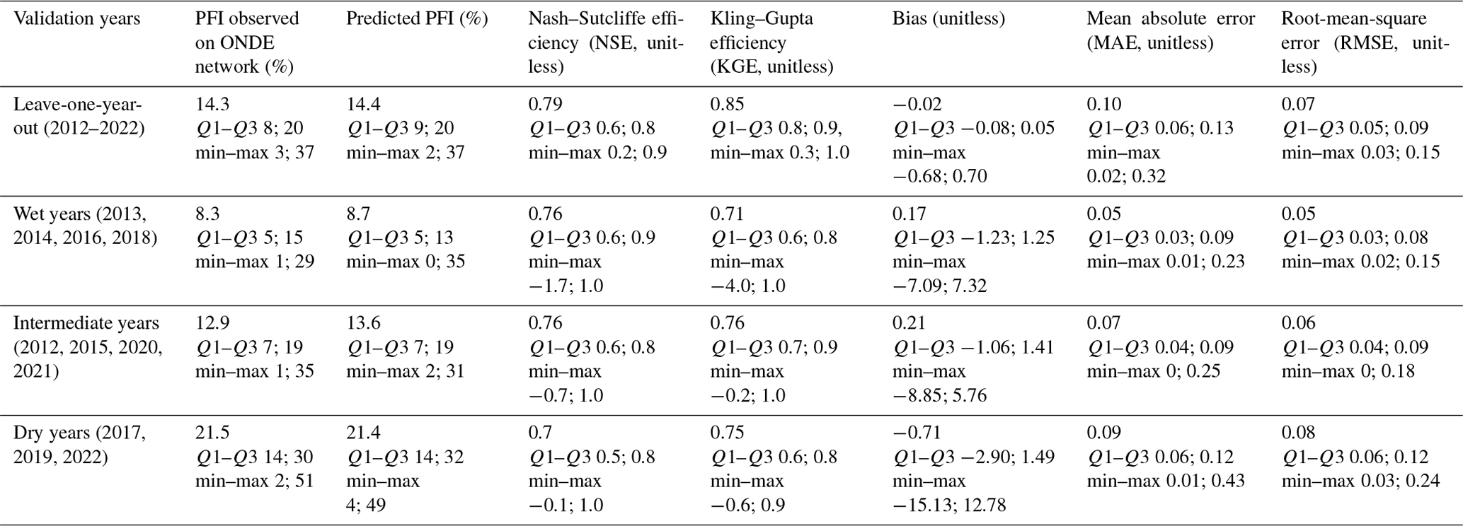
The model performance is assessed using several skill scores: the bias (to detect underestimation or overestimation), the mean absolute error (MAE, to quantify the magnitude of prediction errors), and the root-mean-square error (RMSE, which provides a quadratic estimation that assigns relatively higher weight to large errors). Additionally, the Nash–Sutcliffe model efficiency (NSE) coefficient is computed to compare the variance of the estimation error to the variance of the observed time series (Nash and Sutcliffe, 1970). The Kling–Gupta efficiency (KGE) complements the NSE metric as KGE is the Euclidean distance between observed and estimated PFI, computed using the coordinates of bias, standard deviation, and correlation (Gupta et al., 2009). The leave-one-year-out analysis results are obtained by averaging the validation metrics computed for each year.

3.4 Selecting simulation points for PFI projections under climate change

The modelling framework suggested by Beaufort et al. (2018) and Sauquet et al. (2021) was applied to the 75 HER2s under regional climate projections to assess the potential impact of climate change on flow intermittence dynamics.

Discharge data derived from the Explore2 database are used as input for the logistic regression models introduced in Sect. 3.1. However, not all the stations in the HydroPortail database have been simulated by the hydrological models. To overcome this co-location problem, the choice is made to identify the simulation points closest to the 1008 gauging stations selected for the diagnosis in Sect. 3.2 (Fig. 3). The conditions of the application experiment are thus similar to the ones of the diagnostic experiment. A constraint is applied to ensure that no simulation point is assigned multiple times unless there is no alternative point within a 50 km distance from the gauging station (Appendix D). This selection is made independently for each hydrological model. Only 483 points are assigned for the J2000 model because this model simulates streamflow only for the Loire and Rhône river basins.

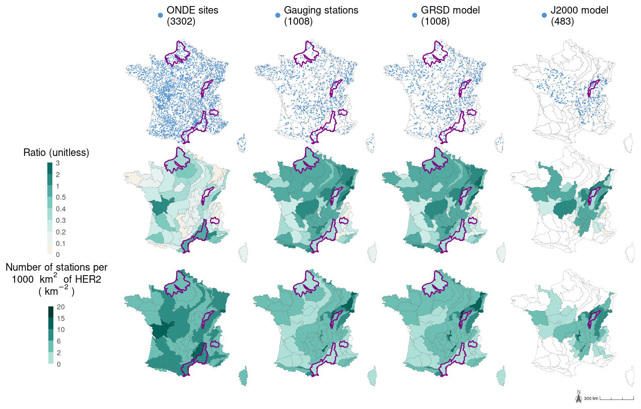
Figure 3 Location of the 3302 ONDE sites, the 1008 gauging stations selected from the HydroPortail database, and the Explore2 simulation points selected for the GRSD and J2000 hydrological models (line 1). The maps on the second line show the ratio between the sum of the catchment areas defined by the gauging stations or the simulation points and the surface area of the HER2 they intersect (line 2). These catchment areas may overlap, and their sums are computed without considering their spatial distribution. The maps on the third line show the density of gauging stations or simulation points (line 3). The same results are available for the other hydrological models in Appendix E.

3.5 Constructing synthetic non-exceedance frequency curves for PFI projections

In our framework, non-exceedance frequency curves must be computed for each simulation point prior to PFI estimation. To avoid problems of extrapolating the non-exceedance frequency of discharge values outside the range of historical flows when performing PFI projection under changing climate, we decided to build synthetic flow time series with a period length of 169 years that combine the historical discharge data simulated with SAFRAN over the period 1976–2022 with discharge data simulated by the different RCP–GCM–RCM–hydrological models modelling chains over the period 1976–2100. This concatenation is made independently for each modelling chain and simulation point. As a consequence, while the assessment of the performance of PFI logistic regression models under the current climate is conducted using observed discharge data that can be unbalanced (i.e. covering different observation periods) due to heterogeneous data availability across stations (see Sect. 3.3), the calibration used for projecting PFI under future climate scenarios relies on standardized and balanced synthetic time series which ensures the consistency of the modelling across simulation points and modelling chains.

Finally, each synthetic discharge time series generated by a specific RCP–GCM–RCM–hydrological models chain results in a non-exceedance frequency curve which is used thereafter to calibrate a logistic regression (Eq. 1).

3.6 Recalibrating logistic regressions and projecting PFI under climate scenarios

Before being applied to future climate conditions, the logistic regression model of Eq. (1) needs to be recalibrated with past discharges simulated by each hydrological model (here discharges simulated by the different hydrological models using SAFRAN reanalysis data available during the period 2012–2022 are used). The resulting logistic regressions are then re-evaluated for each hydrological model using the median of the bias, MAE, RMSE, NSE, and KGE skill scores over all RCP–GCM–RCM modelling chains.

Finally, after re-calibration, these logistic regressions are used to project PFI based on discharge data simulated for both the historical period (1976–2004) and the projection period (2005–2100) under various climate scenarios (RCP2.6, RCP4.5, and RCP8.5).

3.7 Assessing changes in PFI and associated uncertainties

We compare PFI between a reference period (1976–2005) and medium-term (2041–2070) and long-term (2070–2099) horizons. Results are presented at the HER2 scale across France and discussed in more details for four HER2s (Fig. 1), deliberately selected to represent contrasting hydro-climatic conditions and behaviours: “Haute Normandie Picardie” (HER2-57, North, oceanic temperate climate), “Plaine de Bourgogne” (HER2-81, Northeast, continental temperate climate), “Massif de l'Oisans” (HER2-12, Alps, mountainous climate), and “Plaine méditerranéenne” (HER2-105, Southeast, Mediterranean climate). In the rest of the article, “dry periods” of HER2s are defined as the period of the year when PFI is greater than 20 %. For each HER2, the changes in intensity and seasonality of flow intermittence for 2041–2070 and 2070–2099 relative to 1976–2005 are characterized using the mean daily PFI between July and October (mPFI_7–10) and the median of the first and last days (respectively, Tf and Tl) of the year with PFI exceeding 20 %.

The analysis of the uncertainty propagation in the modelling framework is examined using the QUALYPSO method, applied to the national average of mPFI_7–10 (mPFI_7–10[France]), weighted by HER2 areas and obtained under RCP2.6, RCP4.5, and RCP8.5 climate change scenarios (Evin et al., 2019, 2021). The QUALYPSO method is used to characterize the changes in mPFI_7–10[France] by estimating its ensemble mean over all the projections, as well as the total uncertainty associated with this set of projections, the contribution of the various sources of uncertainty (RCP, GCM, RCM, hydrological models, residual and internal climate variability) to the total uncertainty, and the main effect of each individual model and its contribution to the total uncertainty. The contribution of each component to the total uncertainty is estimated as its fixed effect in a linear regression model, which adjusts for imbalances in the number of simulations across components within modelling chains (Appendix F).

A multi-model index of agreement (MIA) is also computed on mPFI_7–10 time series to highlight convergence in changes over the projections (Tramblay and Somot, 2018):

$$\begin{array}{}\text{(3)}& \mathrm{MIA}={\displaystyle \frac{\mathrm{1}}{n}}{\sum }_{k=\mathrm{1}}^n{i}_k,\end{array}$$

where n is the number of projections, i_k=1 for a significant positive trend of the mPFI_7–10 according to the Mann–Kendall test (with α = 0.1), $i_k=-\mathrm{1}$ for a significant negative trend, and i_k=0 for no significant trend.

4 Results

4.1 Data pre-processing

The 3302 ONDE sites are located in small streams, while gauging stations in France are monitoring medium-size catchments (Van Meerveld et al., 2020). In addition, all Explore2 simulation sites have a drainage area larger than 64 km². Unsurprisingly, there is little overlap between the distribution of areas drained by ONDE sites (median: 24 km²; quartiles Q1–Q3: 12–50) and those drained by the two sets of 1008 gauging stations (median: 173 km²; Q1–Q3: 85–396) and 1008 simulation points (median: 178 km²; Q1–Q3: 95–400; Appendix Fig. G1). ONDE sites, gauging stations, and simulation points are located at similar elevations (overall median: 168 m; Q1–Q3: 75–308; Appendix Fig. G2). The drainage areas of ONDE sites, gauging stations, and simulation points represent respectively a median coverage of 21 % (Q1–Q3: 15–35), 54 % (Q1–Q3: 31–94), and 55 % (Q1–Q3: 32–96) of the HER2 areas. This corresponds to a median number of 6.1 sites (Q1–Q3: 5–8), 3.6 stations (Q1–Q3: 1.9–5.7), and 3.7 simulation points (Q1–Q3: 2–6) per 1000 km² of HER2 (Fig. 3). These statistics highlight the question of representativeness of the ONDE sites despite the even coverage of the ONDE network.

4.2 Model performance

The logistic regressions calibrated using observed flows accurately predict PFI under current climate conditions (Fig. 4; Appendix Fig. H1). The median performance across HER2s is, for example, 0.85 for KGE (Q1–Q3: 0.77–0.89) and 0.79 for NSE (Q1–Q3: 0.64–0.84) when the leave-one-year-out cross-validation is considered. The KGE skill score exceeds 80 % in 50 out of 75 HER2s, and the bias is very low. The best performances are observed in sedimentary plains and in Aquitaine, while weaker performances are obtained in mountainous areas such as the Alps, the Massif Central and the Pyrenees. The mean absolute error and RMSE show that the largest absolute deviations between observations and predictions occur in the southeastern part of France. This result is consistent with previous findings (e.g. Fig. 3 in Sauquet et al., 2021): (1) the performance of the logistic regressions is partly correlated with the level of intermittence, and (2) no-flow conditions which mainly occur in winter due to freezing in the Alps are not captured by the ONDE network. Observed values of mPFI_7–10 range between 3 % and 37 % (median: 14.3 %) across France, while values of mPFI_7–10 obtained with SAFRAN range between 2 % and 37 % (median: 14.4 %). The modelling approach is able to reproduce the spatial pattern of flow intermittence (Fig. 4), although the results obtained with the DSST show less satisfactory performance (Appendix Fig. H2 and Table H1). The two skill scores KGE and NSE are sensitive to wet, intermediate, and dry conditions, while the other skill scores show no major change. The values of RMSE and MAE skill scores do not increase much when the calibration dataset is stratified based on climate conditions, which indicates that the proposed model is quite robust against climate fluctuations. The bias, however, indicates an underestimation of PFI in the southwest and in the north during dry years. This lower performance is partly due to a reduced number of years used for calibration purposes and to the difficulty in extrapolating the logistic regression equations under unobserved climate conditions.

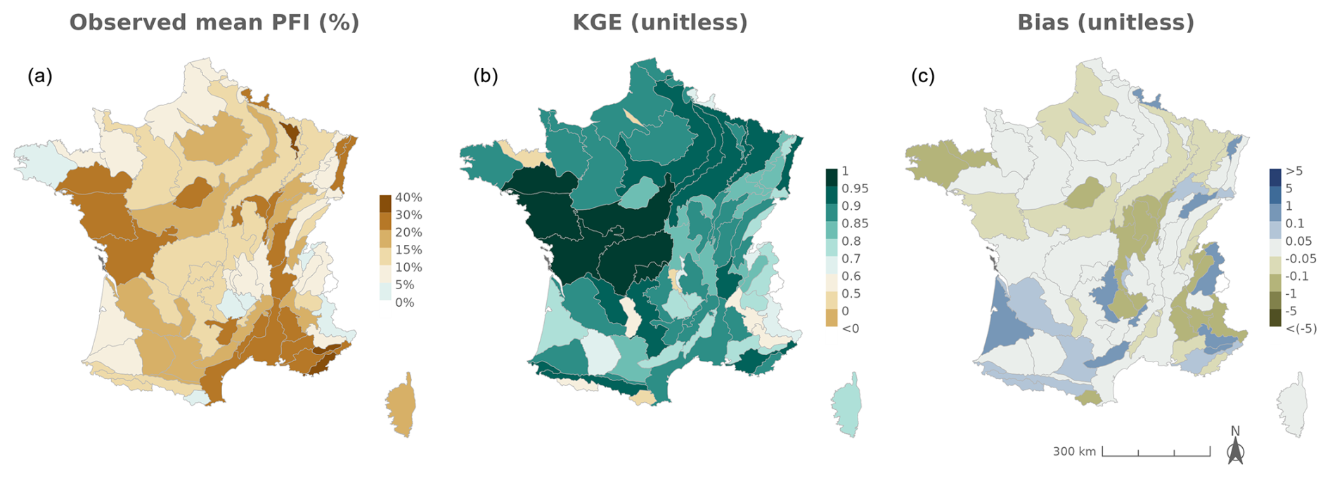
Figure 4 Leave-one-year-out cross-validation assessing the calibration of the logistic regressions using discharge measurements from gauging stations. From left to right: observed mean PFI measured during the calibration period (2012–2022, a), Kling–Gupta efficiency (KGE, b), and absolute bias of PFI predictions (c).

The logistic regressions fitted with discharge data simulated by hydrological models also accurately reconstruct PFI from May to September. Compared to the results obtained with observed discharge data, the performance is slightly lower due to the inherent imperfections of the SAFRAN reanalysis compared to the observed climate (Figs. 5, 6; Table 1; Appendix I). The inter-HER2 and inter-projection median estimated mPFI_7–10 across France is 11.3 %–13.5 % depending on hydrological models, which is close to the 14.3 % value (Q1–Q3: 8.4–20.3) derived from the ONDE network. The KGE is slightly lower but exceeds 80 % in more than half of the HER2s using the CTRIP ($\mathrm{38}/\mathrm{75}$), SMASH ($\mathrm{38}/\mathrm{75}$), and GRSD ($\mathrm{43}/\mathrm{75}$) models. The inter-HER2 median of the NSE skill score (calculated for all RCP–GCM–RCM modelling chains and for each of these three hydrological models) indicates that between 71 % and 74 % of the variance in mPFI_7–10 is explained by the logistic regressions. The other skill scores do not show a loss of performance (KGE between 0.80 and 0.81, MAE between 0.04 and 0.05, and RMSE between 0.06 and 0.07) when comparing the results of the leave-one-year-out cross-validation obtained using observed and simulated discharge data. Lower performance is observed with the ORCHIDEE and J2000 models, as the KGE exceeds 80 % in only $\mathrm{7}/\mathrm{75}$ and $\mathrm{5}/\mathrm{37}$ HER2s, respectively. Their median KGE (0.60 and 0.69, respectively), NSE (0.49 and 0.62), MAE (0.06), and RMSE (0.08 and 0.09) are lower than the values obtained during calibration using observed flow data, indicating that these two hydrological models seem less sensitive.

Regardless of the hydrological model of interest, the maps of skill scores show spatial patterns that are consistent with the results obtained with observed discharge data (Fig. 6; Appendix I). Both NSE and KGE remain high in the sedimentary plains and the southern part of the country, while they are less favourable in mountainous regions (Alps, Massif Central, and Pyrenees). An overestimation persists in the southwestern part of France, while underestimations of PFI values are found in the northwestern, northern, and southeastern parts of France and are especially pronounced during dry years. The models also successfully reproduce the inter-annual variability in PFI, particularly the alternation of dry (e.g. 2019) and wet (e.g. 2015) years (Fig. 5). Thus, the modelling chains demonstrate their ability to simulate PFI over the period 2012–2022 and are therefore deemed reliable to attempt projecting changes in flow intermittence under modified climate conditions. However, note that PFI values are slightly underestimated when the logistic regressions are calibrated on the driest years and then applied to wetter years. This suggests that our future projections are likely to be biased in the same way, since the calibration is based on current conditions before applying the regression models to a potentially drier future climate.

Table 1 Evaluation of the logistic regressions calibrated using observed discharge data (results of the cross-validation) and using flows simulated by the CTRIP, GRSD, J2000, ORCHIDEE, and SMASH hydrological models. Statistics of the skill scores are summarized by medians and the first and the third quartiles (Q1–Q3, into brackets) across all HER2s.

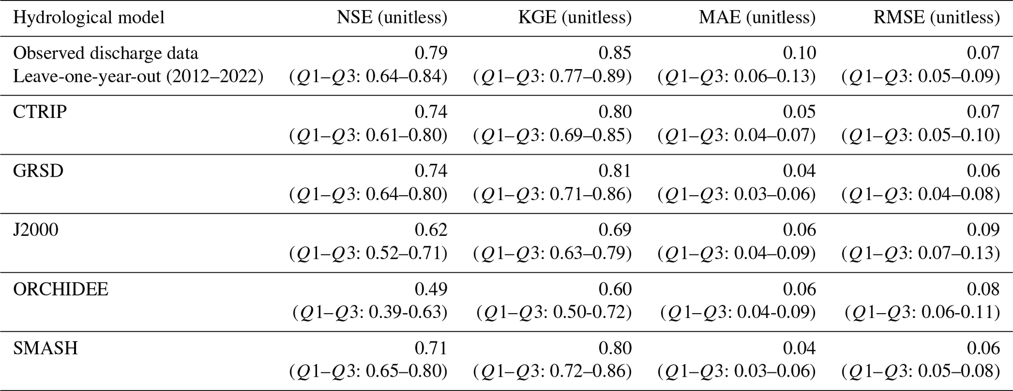
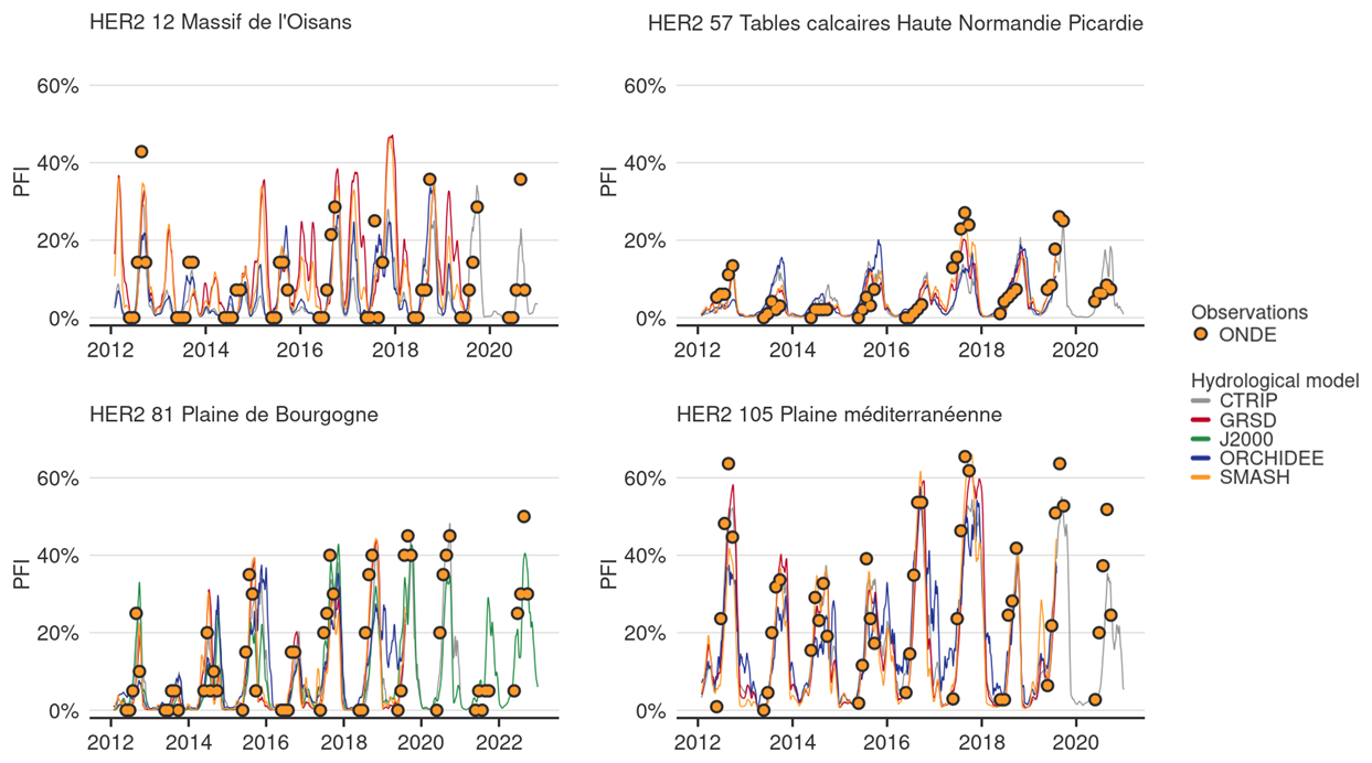
Figure 5 Time series of PFI for the four HER2s selected for illustrative purposes. Dots and lines are observed PFI derived from the ONDE network and estimated PFI computed by the logistic regressions using simulated discharge by each hydrological model, respectively.

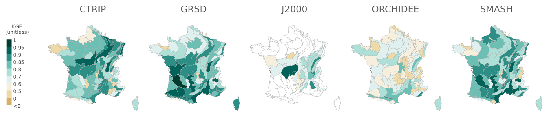
Figure 6 Kling–Gupta efficiency (KGE) assessing the calibration of logistic regression using discharge simulated by each hydrological model with SAFRAN-based simulations available during the 2012–2022 period.

4.3 Flow intermittence projections

The logistic regressions fitted for each HER2 are applied to derive the PFI values from the historical (1976–2004) and future (2005–2100) discharges simulated by the hydrological models forced by RCP–GCM–RCM climate projections over the period 1976–2100.

Figure 7 shows the evolution of mPFI_7–10 and of the start date (Tf) and end date (Tl) of the dry period for 2041–2070 and 2070–2099 compared to 1976–2005. The results are illustrated in Fig. 7 with the median projection given by the GRSD model (see Appendix Figs. J1–J4 for other models) under RCP2.6, RCP4.5, and RCP8.5 climate scenarios. Table 2 details the same results for the four HER2s under RCP8.5.

Overall, the average PFI shows an increase, indicating a gradual intensification of dry periods over the 21st century under the RCP4.5 and RCP8.5 scenarios. The inter-HER2 and inter-projection median of mPFI_7–10 calculated at the national scale (mPFI_7–10[France]) for the baseline period 1976–2005 ranges from 10 % to 12 % depending on the hydrological model. However, the median projection of mPFI_7–10 during 1976–2005 is higher than 20 % in 12 to 20 of the 75 HER2s (depending on the hydrological model), although it does not exceed 42 % in any HER2. Under RCP8.5, mPFI_7–10[France] could reach values between 13 % and 21 % by the middle of the century 2041–2070 and between 16 % and 29 % by the end of the century 2070–2099. By this time, six HER2s could have inter-projection medians of mPFI_7–10 exceeding 50 % according to at least two hydrological models: four in the southeast of France, one in the southwest, and one in the northwest of France. Under RCP4.5, changes are more moderate by the end of the century 2070–2099, with mPFI_7–10[France] ranging between 14 % and 20 %. The spatial pattern of the changes is not uniform but looks similar between RCP8.5 and RCP4.5. A strengthening divide between the southwest and the northeast of the country is projected. Regions already prone to intermittence are expected to experience an increase in this phenomenon under both emission scenarios. The ratio of the ensemble median of mPFI_7–10 at the end of the century compared to the baseline period revolves around 1.4 for RCP4.5 and 1.9 for RCP8.5. Mountainous regions see the intensity of summer dry periods increase but remain relatively spared.

Shifts of the start and the end of the dry period are partly correlated with changes in mPFI_7–10 (Fig. 7). It appears that climate change results in both earlier and later dry periods in a fairly symmetrical manner: dry periods are advanced and extended but with different sensitivities structured along a north–south gradient. Under RCP8.5 climate conditions, the dry periods are projected to get (on median) longer in southern France at the end of the century. According to at least two hydrological models, the highest shifts of Tf or Tl could exceed 5 weeks in several mountainous HER2s (four HER2s in the Alps, three in the Pyrenees, two in the Jura). In contrast in the northern part of France, the dry periods could be advanced and extended by only 1 or 2 weeks, as observed in HER2-81 “Plaine de Bourgogne” (Table 2). HER2-28 could be one of the most affected in the north due to its impermeable sandy-clay formations, which differ from the neighbouring sedimentary formations. One can note a change in seasonality for the HER2-12 “Massif de l'Oisans” located in the Alps (Fig. 8, example with the GRSD hydrological model). No-flow events were concentrated in winter (retention of water in the snow cover) during the historical period. Under climate change, temperature will be higher leading to less snowfall and more runoff in the river network during winter. The river flow regime will be more sensitive to losses by evapotranspiration, and finally no-flow conditions will likely occur in summer by the end of the 21st century.

Table 2 Statistics of flow intermittence characteristics for the four illustrative HER2s under RCP8.5. The minimum (min), median (med), and maximum (max) are the ensemble minimum, median, and maximum across all the projections and hydrological models. Nb Days PFI >20 %: number of days in dry periods (period of the year when PFI exceeds 20 %).

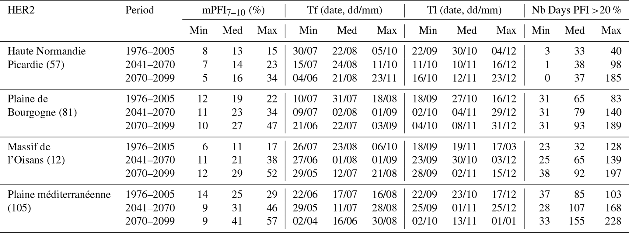
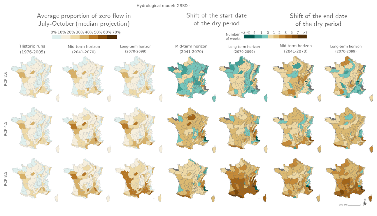
Figure 7 Ensemble median mPFI_7–10 (columns 1 to 3) and ensemble median shift of the start date Tf (columns 4 and 5) and the end date Tl (columns 6 and 7) of the dry period over the two periods 2041–2070 and 2070–2099 under the three RCPs for the GRSD hydrological model, relative to the baseline period 1976–2005. The shift, expressed in weeks, takes a positive value when the duration of the dry period increases. Grey HER2s had no period with a PFI >20 % during the reference period. The same results are available for the other hydrological models in Appendix Figs. J1–J4.

Figure 8 Seasonal pattern of PFI for the periods 1976–2005, 2041–2070, and 2070–2099 under RCP2.6, RCP4.5, and RCP8.5 scenarios for the GRSD hydrological model in the Alps (HER2-12). The storylines highlighted in this figure are introduced in Appendix J. The same results are available for HER2-57, HER2-81, and HER2-105 and for the other hydrological models in Appendix Figs. J5–J21.

4.4 Uncertainties in hydro-climatic projections and their impact on PFI projections

Figure 9 illustrates the results of the uncertainty analysis, showing the uncertainty range of mPFI_7–10[France] throughout the 21st century. These results confirm that dry conditions may occur more frequently in a changing climate, with a 22 % projected increase in mPFI_7–10[France] by the end of the century. The total uncertainty of mPFI_7–10[France] over all projections results from the accumulation of uncertainties related to RCP scenarios, GCMs and RCMs, hydrological models, residual variability, and internal variability. The confidence interval, and therefore the extent of change, increases over the course of the 21st century due to the divergent results of the modelling chain. This finding is consistent with studies using a similar methodology to assess the uncertainty of panels of flow projections (Evin et al., 2019; Aitken et al., 2023).

The contribution of each component to the total uncertainty varies over time. The fraction of total variance due to residual variability is small and remains stable over time. The main part of the uncertainty in climate change responses is thus explained by RCP, GCM, RCM, and hydrological models. In addition, the contribution of the internal variability is highly predominant and represents more than 75 % of the total uncertainty until the mid-century. This contribution then decreases with time as the total uncertainty increases. It becomes less than 50 % of the total uncertainty by the end of the century but remains the greatest contributor to the total uncertainty over the whole simulation period.

Regarding the spatial distribution of the different contributions to the total uncertainty, it appears that climate models are a predominant source of uncertainty and that they are distributed in a spatially heterogeneous manner over France. The uncertainty related to the RCP scenarios increases over time and becomes predominant in the south, surpassing uncertainties related to other steps of the modelling chain (GCM, RCM, and hydrological models). In the mountainous regions, differences between results obtained with RCP4.5 and RCP8.5 are clearer by the end of the century, leading to a contribution of RCP to the total uncertainty reaching 20 % at the end of the century. In northern France, the contribution of RCP to the uncertainty is lower compared to hydrological model, GCM, or RCM contributions. Uncertainty related to hydrological models is also spatially structured, with greater uncertainty in the northwestern part of France.

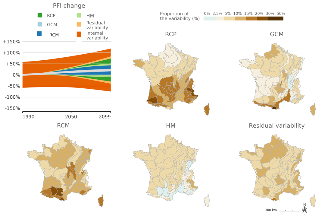
Figure 9 Decomposition of the effects contributing to the variance of projections for relative changes (unitless) of mPFI_7–10[France]. In the top-left graph, the grey line and the coloured areas respectively show the climate change response and the contribution of time for each step of the modelling chain to the 90 % confidence interval. For each model uncertainty and internal variability component, the vertical extent of the corresponding area is proportional to the fraction of total uncertainty explained by the component.

4.5 Agreement between changes

Despite uncertainties about the intensity of change, PFI projections still show a good degree of convergence in the direction of change when considering all climate projections driving each hydrological model individually, as well as in the overall convergence of PFI projections (Fig. 10). MIA values are first calculated independently for each hydrological model before all projections are combined for multi-model assessment.

Figure 10 highlights spatial contrasts of the MIA multi-model approach: unsurprisingly, the projections of mPFI_7–10 are more uncertain in the northern part of France. The climate change signal on the proportion of dry periods is not homogeneous across France, with significant uncertainties remaining for the northern part.

The agreement of projections is high for the GRSD and SMASH models across France (MIA values close to +100 % under RCP8.5 in Fig. 10 and +80 % under RCP4.5; see Appendix K). In contrast, CTRIP, J2000, and ORCHIDEE suggest contrasted regional impacts of climate change on PFI under RCP4.5, with a reduction in the mPFI_7–10 in the northern part of France, indicating a differentiated sensitivity of hydrological models to climate changes. This trend is also observed for ORCHIDEE under RCP8.5, while the other models agree on an increasing drying.

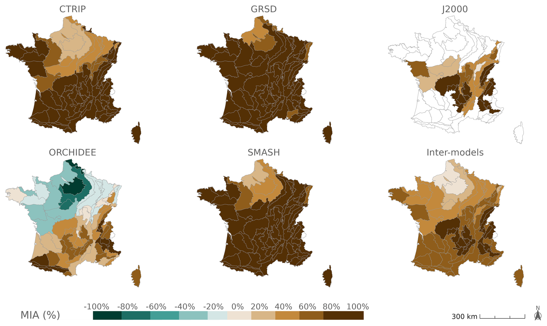
Figure 10 Agreement between projections of mPFI_7–10 for each hydrological model and inter-model agreement on the change signal of mPFI_7–10 under the RCP8.5 scenario.

5 Discussion

5.1 Modelling framework and assumptions

This study presents projections of the PFI in small streams by HER2s in France over the 21st century. It extends the previous analysis of Sauquet et al. (2021) on the 2012–2018 period by exploiting an extensive national dataset of stream intermittence observations collected on low-order streams (3302 observation sites), which are the most affected by shifts from perennial to intermittent flows (Reynolds et al., 2015; Dhungel et al., 2016). For the first time, we project the future evolution of the PFI using discharge data obtained from 5 hydrological models with conceptual (GRSD, SMASH), surface (CTRIP, ORCHIDEE), or process-oriented distributed (J2000) structures, under a multitude of possible climate scenarios informed by 17 pairs of CMIP5 GCM–RCM models.

The results of this study should be interpreted within the context of its underlying assumptions. Firstly, the study focuses on unregulated streams to characterize the “natural” hydrology (i.e. without considering water abstraction by anthropogenic activities or the impact of hydraulic engineering structures). This assumption was made in the Explore2 project, which provides the input streamflow simulations. Nevertheless, global water model simulations including direct human impacts by Döll and Zhang (2010) or Gudmundsson et al. (2021) concluded that ecologically relevant flow characteristics will be more altered by climate change than by withdrawals and dams. However, we believe that quantitatively estimating the extent to which flow intermittence is due to direct anthropogenic stressors is crucial. Such an estimation could improve our projections of flow intermittence and inform decision-making aimed at regulating and preventing water stress situations for populations.

Secondly, groundwater levels are not incorporated into the model, although they could potentially enhance the accuracy of the projections. Indeed, similar logistic regression models were used in Beaufort et al. (2018), and they incorporated groundwater levels measured by piezometers. Likewise, in Beaufort et al. (2019), climate, hydrological, and morphological data were supplemented with groundwater levels to predict flow intermittence at a local scale. In these studies incorporating subsurface water in the regression models was thought to improve performance, in particular because the contribution of subsurface processes is known to play a decisive role in maintaining baseflow and mitigating flow intermittence. However, information about groundwater levels has not been included in the present study because hydrological projections incorporating groundwater levels have not yet been conducted across the entirety of France (for instance, within the Explore2 project, projections of groundwater levels have only been produced for a restricted set of areas in France).

Thirdly, with only five annual discrete observations of streamflow intermittence over 11 years for the calibration of the logistic regression models, our ability to capture the full range of extremes and variability in these regression models remains imperfect. Yet, visual monitoring remains the most common technique for observing non-perennial streams. An alternative approach would be to consider citizen science to augment our database, although concerns about data reliability persist, in particular because past studies have shown participant agreement rates ranging from 46 % to 70 % (Scheller et al., 2024). Data scarcity necessitated conducting this analysis at the HER2 scale, which nonetheless represents a significant improvement of the spatial resolution by increasing the number of modelling subdomains from 22 to 75 compared to previous studies (Sauquet et al., 2021). In future work, a downscaling process could enhance the usability of PFI projections for local stakeholders in water management.

Fourthly, while projections of no-flow events often exhibit significant uncertainties when derived directly from discharge simulated by hydrological models (Evin et al., 2024; Aitken et al., 2023), this study illustrates how categorical and discrete (in space and time) field observations can be combined with conventional stream gauge data to enhance the understanding of small-stream drying dynamics. In this way, despite the divergences between projections induced by climate data, the agreement within this multi-model approach is relatively strong, indicating a consensus toward increasing PFI throughout the 21st century.

5.2 A consistent signal across projections

This study confirms that logistic regressions properly capture the relationships between flows in large watersheds and the PFI of small streams. These regressions are calibrated and validated using discharge measurements from gauging stations and subsequently using discharge simulated from SAFRAN climate data. Following this second calibration, projections based on regressions consistently indicate an increase in average PFI and a shift in the start and end dates of dry periods under RCP4.5 and RCP8.5 climate projections, suggesting a progressive intensification and extension of dry periods over the 21st century.

These results are consistent with previous studies indicating a transition of many streams from perennial to intermittent regimes (Jaeger et al., 2014; Reynolds et al., 2015; Dhungel et al., 2016; Schneider et al., 2013). In regions already affected by intermittence, an increase in the intensity and duration of drying periods is likely, a phenomenon also anticipated in other areas around the world (Jaeger et al., 2014; Dai et al., 2011). Increasing intermittence and decreasing flow rates are observed in catchment-scale studies: the fraction of time with zero discharge increases from 0.05 % to 4.30 % in a Swiss alpine catchment between 2020–2040 and 2080–2100 (Halloran et al., 2023), while the no-flowing phase could extend by up to 12 d between 1980–2009 and 2030–2059 for a catchment in southern Italy (De Girolamo et al., 2022). This trend is also noticeable on a larger scale, as the monitoring of gauging stations both in five regions with Mediterranean climates around the world between 1980 and 2019 (Carlson et al., 2024) and over 452 rivers on the European continent between 1970 and 2010 (Tramblay et al., 2020) shows that approximately 30 % of them have already experienced drier conditions due to climate change, with modified flow regimes or extended periods of drying.

5.3 Uncertainties in northern France

In the northern part of France, discrepancies between GCM–RCM–hydrological models projections result in higher uncertainties in PFI projections and pronounced geographical contrasts on the multi-model-based MIA map (Fig. 10). Part of these uncertainties can be attributed to the underestimation of PFI in this region, particularly during dry years (Sect. 4.2, Appendix Fig. H2, and Table H1). However, the primary source of these uncertainties likely stems from uncertainties in future rainfall patterns in this region where the majority of Explore2 projections indicate an increase in winter rainfall and winter mean flows (for 8 out of 9 hydrological models) and a decrease in summer precipitation (Evin et al., 2024; Sauquet et al., 2024). The annual precipitation by the end of the century remains uncertain due to the compensatory effect between increased winter recharge and an increased evapotranspiration (Ribes et al., 2022; Douville et al., 2021). As a result, some hydrological models predict a shortening of the dry period for certain northern HER2s, including under RCP8.5. Similar uncertainties are observed along the east coast of the USA, where precipitation changes could turn intermittent streams into perennial ones (Dhungel et al., 2016), while alternative climate change scenarios projected that by the 2040s, approximately half of the streams in Washington State would shift from snow-fed to rain-fed, resulting in reduced annual discharge (Reidy Liermann et al., 2012).

5.4 Transformation of the snowmelt regime in the Alps

The mountain ranges could be moderately affected by the increased probability of dry conditions, consistent with our previous modelling efforts (Sauquet et al., 2021), but our projections anticipate two specific phenomena in these regions. First, the Pyrenees are more affected than the other mountain ranges, with significant changes impacting the massif and the dependent basins in southwestern France. Additionally, alpine HER2s will probably undergo hydrological regime changes. Higher winter temperatures will lead to reduced snowfall and snow-related intermittence. This snowpack reduction will also reduce groundwater recharge by spring melt. In addition, since soils tend to retain less water in summer due to more intense and brief rainstorms (Rutkowska et al., 2023), an increased summer intermittence is expected despite increasing summer precipitations. Using 16 hydrographic variables describing the magnitude, frequency, timing, duration, and rate of change of the flow regime at 59 primarily selected sites with a Strahler order of 5, Dhungel et al. (2016) also observed the reduction in the snowmelt regime at two Rocky Mountain sites under climate change. Halloran et al. (2023) also conclude that groundwater will play an increasingly important role in ensuring flow in alpine streams and that the shift from perennial to intermittent could occur for alpine streams over the course of the current century.

Furthermore, the reduction in the snowmelt regime in the Alps indicates that we can still make projections consistent with the literature beyond the calibration period (May to September). More generally, the hypothesis of temporal transferability of the models is a strong assumption in data exploitation, as it assumes that climate models, statistical adjustment methods, and hydrological models can simulate the behaviour of the systems they represent in a future hydro-climatic context that is very different from the one in which they were developed (Evin et al., 2024). In this context, it is important to recall the risk that the projections may be underestimated, as demonstrated by the validation of logistic regressions calibrated on wetter years compared to dry years.

6 Conclusion

This study assesses the changes in the intermittency of river flows across France in the context of climate change. For the first time, multi-model and multi-scenario hydro-climatic projections are used as a predictor to explore the possible evolution of the daily probability of flow intermittency at the scale of (level-2) hydro-ecoregions. Leveraging monthly monitoring of small streams over 10 summers, we calibrated logistic regressions to transform hydrological projections of large watersheds into regional proportions of flow intermittence for the 21st century. Under both RCP4.5 and RCP8.5 scenarios, robust signals indicate an intensification of dry events, marked by an increased probability of flow intermittence and longer dry periods throughout the year. These changes are projected to be more pronounced in southern France, with greater uncertainty in the northern half of the country. Mountain areas could remain relatively spared from summer dry periods, but shifts in hydrological regimes are anticipated. By the end of the century under RCP8.5, dry-stream phenomena along the Atlantic coast could surpass those currently observed in the Mediterranean region by the usual monitoring campaigns. The evolution of droughts and reduced water availability suggested by these results could lead to significant ecological impacts, including alterations in the structure and function of freshwater ecosystems (such as changes in microbial activity and habitat loss), shifts in soil chemistry, increased carbon and solute fluxes, and sediment mobilization (Geris et al., 2015).

Appendix A: Explore2 modelling

Table A1 Global and regional climate model combinations driving the Explore2 hydrological models selected for PFI simulation in the 21st century.

Appendix B: Sensitivity analysis of the duration of flow measurement interval used as input for the logistic regression to calculate the PFI

A sensitivity analysis was performed to fix the time window of daily discharge that optimizes the calibration of logistic regressions presented in Sect. 3.1. The calibration and validation were performed using the leave-one-year-out method, detailed in Sect. 3.3. The model performance was assessed using the Kling–Gupta efficiency (KGE) (Gupta et al., 2009). The KGE values for the different HER2s are summarized using boxplots for each tested window size. The $[j-\mathrm{6};j]$ window was selected because it corresponds to the highest median KGE score, the narrowest interquartile range, and the highest minimum KGE.

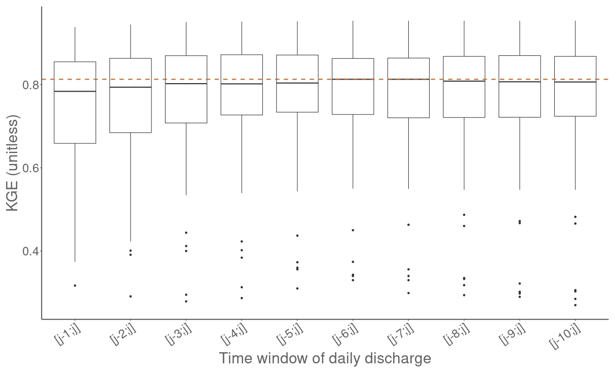
Figure B1 Kling–Gupta efficiency (KGE) computed on results obtained by leave-one-year-out validations, testing the sensitivity to the time window of daily discharge used for calibrating the logistic regressions. Boxes represent the quartiles Q1 and Q3, the whiskers extend up to 1.5 times the interquartile range above Q3 and below Q1, and points located beyond the whiskers are displayed individually. The dashed line represents the median KGE of the $[j-\mathrm{6};j]$ window.

Appendix C: Separation of dataset based on dry, intermediate, and wet years

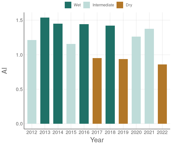
The data from ONDE sites used for validation were collected between May and September over 11 years from 2012 to 2022. The robustness of the model was assessed through a validation process involving three sets of dry, intermediate, and wet years. For each test, model calibration was performed using the years excluded from the validation set.

The hydrological years are distributed into three equal groups of hydrological years (dry years, intermediate years, and wet years) according to the annual aridity index, calculated at the national scale. The aridity index AI was given by the ratio between the total annual precipitation and potential evapotranspiration from 1 August of the previous year to 31 July of the current year (Barrow, 1992; Fig. C1). A set of dry years was formed using hydrological years where potential evapotranspiration exceeded annual precipitation (AI <1 for 2017, 2019, and 2022). Two sets were then created: the four years with AI greater than 1.4 were classified as wet years (2012, 2015, 2020 and 2021), and the remaining four years with AI between 1.15 and 1.37 were classified as intermediate years (2013, 2014, 2016, 2018).

Figure C1 Aridity index for the hydrological years 2012 to 2022.

Appendix D: Assignment of simulation points

After establishing the models' reliability through validation at secure monitoring stations, the next step involved extrapolation, which entailed linking these monitoring sites to the nearest simulation points in Explore2 to project future hydrological scenarios while preserving the existing data structure. The proximity between gauging station A and a simulation point in the Explore2 project is measured by the distance.

$$\begin{array}{}\text{(D1)}& \begin{array}{rl}& \mathrm{Dist}(A,B)\\ & =\sqrt{\left(X\right(A)-X(B){)}^{\mathrm{2}}+(Y\left(A\right)-Y\left(B\right){)}^{\mathrm{2}}+(\mathit{\alpha }\times \mathrm{\Delta }{S}_{\mathrm{rel}}{)}^{\mathrm{2}}}\end{array}\end{array}$$

Here, (X(A)Y(A)) and (X(B)Y(B)) are coordinates of A and B (in km), respectively, and Surf(A) and Surf(B) are the drainage areas of A and B, respectively, that are used to compute the relative difference between the drainage areas (absolute value).

$$\begin{array}{}\text{(D2)}& \mathrm{\Delta }{S}_{\mathrm{rel}}=\mathrm{2}\times {\displaystyle \frac{\left|\mathrm{Surf}\right(A)-\mathrm{Surf}(B\left)\right|}{\left|\mathrm{Surf}\right(A)+\mathrm{Surf}(B\left)\right|}}\end{array}$$

The coefficient α is used to balance the importance of geographical distance and the relative difference in surface, and it was set to 100.

Appendix E: Location of the ONDE sites, the gauging stations, and the Explore2 simulation points selected for each hydrological model

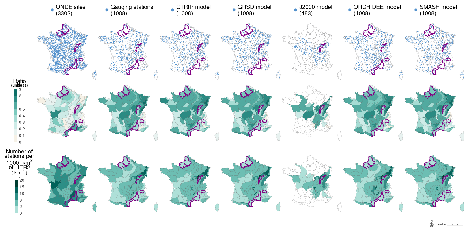
Figure E1 Location of the 3302 ONDE sites, the 1008 gauging stations selected from the HydroPortail database, and the Explore2 simulation points selected for each hydrological model (line 1). Maps on the second and third lines respectively show the ratio between the sum of the catchment areas defined by the gauging stations or the simulation points and the surface area of the HER2 they intersect (line 2), and the density of gauging stations or simulation points (line 3).

Appendix F: QUALYPSO method

The QUALYPSO method is applied to the multi-scenario multi-model ensembles of projections of the national average of mPFI_7–10 (mPFI_7–10[France]), weighted by HER2 areas and obtained under RCP2.6, RCP4.5, and RCP8.5 climate change scenarios. According to Evin et al. (2019), we assume that the variable ${\mathrm{mPFI}}_{\text{7–10}i,j,k,l}^{\ast }\left(t\right)$ characterizes the change in mPFI_7–10 between a year t and the control year c (e.g. c=1990 in this study) for a given combination of RCP scenario i, GCM j, RCM k, and hydrological model l:

$${\mathrm{mPFI}}_{\text{7–10}i,j,k,l}^{\ast }\left(t\right)={\mathrm{mPFI}}_{\text{7–10}i,j,k,l}\left(t\right)-{\mathrm{mPFI}}_{\text{7–10}i,j,k,l}\left(c\right).$$

The change in mPFI_7–10 can be split up into

$${\mathrm{mPFI}}_{\text{7–10}i,j,k,l}^{\ast }\left(t\right)={\mathit{\phi }}_{i,j,k,l}^{\ast }\left(t\right)+{\mathit{\eta }}_{i,j,k,l}^{\ast }\left(t\right),$$

where ${\mathit{\phi }}_{i,j,k,l}^{\ast }\left(t\right)$ is the climate change response of the RCP–GCM–RCM–hydrological models combination, and ${\mathit{\eta }}_{i,j,k,l}^{\ast }\left(t\right)$ is the deviation from the climate change response for this RCP–GCM–RCM–hydrological models combination as a result of internal variability, representing natural and stochastic variability in the climate system.

For each time t, the climate change response characterized by ${\mathit{\phi }}_{i,j,k,l}^{\ast }\left(t\right)$ of any RCP–GCM–RCM–hydrological models combination can be expressed as

$${\mathit{\phi }}_{i,j,k,l}^{\ast }\left(t\right)=\mathit{\mu }\left(t\right)+{\mathit{\alpha }}_i\left(t\right)+{\mathit{\beta }}_j\left(t\right)+{\mathit{\gamma }}_k\left(t\right)+{\mathit{\theta }}_l\left(t\right)+{\mathit{\epsilon }}_{i,j,k,l}\left(t\right),$$

where μ(t) is the ensemble mean climate change response, α_i(t) is the main effect of emission scenario i (i.e. the mean deviation of RCP scenario i from μ(t)), β_j(t) is the main effect of GCM j, γ_k(t) is the main effect of RCM k, θ_l(t) is the main effect of the hydrological model l, and ${\mathit{\epsilon }}_{i,j,k,l}\left(t\right)={\mathit{\phi }}_{i,j,k,l}^{\ast }\left(t\right)-\mathit{\mu }\left(t\right)-{\mathit{\alpha }}_i\left(t\right)-{\mathit{\beta }}_j\left(t\right)-{\mathit{\gamma }}_k\left(t\right)-{\mathit{\theta }}_l\left(t\right)$ corresponds to residual terms. For each year t, ${\mathit{\epsilon }}_{i,j,k,l}\left(t\right)$ are assumed to be independent and identically distributed over all scenarios, GCMs, RCMs, and hydrological models and to follow normal distributions, with mean 0 and variance σ²(t).

If ${\mathit{\phi }}_{i,j,k,l}^{\ast }\left(t\right)$ and ${\mathit{\eta }}_{i,j,k,l}^{\ast }\left(t\right)$ are assumed to be independent, the total variance of the change variable ${\mathrm{mPFI}}_{\text{7–10}i,j,k,l}^{\ast }\left(t\right)$ is given by

$$\mathrm{Var}\left({\mathrm{mPFI}}_{\text{7–10}i,j,k,l}^{\ast }\left(t\right)\right)=\mathrm{Var}\left({\mathit{\phi }}_{i,j,k,l}^{\ast }\left(t\right)\right)+\mathrm{Var}\left({\mathit{\eta }}_{i,j,k,l}^{\ast }\left(t\right)\right),$$

where $\mathrm{Var}\left({\mathit{\eta }}_{i,j,k,l}^{\ast }\left(t\right)\right)$ is the uncertainty associated with internal variability in ${\mathrm{mPFI}}_{\text{7–10}i,j,k,l}^{\ast }\left(t\right)$.

$\mathrm{Var}\left({\mathit{\phi }}_{i,j,k,l}^{\ast }\left(t\right)\right)$ is the uncertainty in the climate change response, calculated as the sum of different uncertainty components.

$$\begin{array}{rl}\mathrm{Var}\left({\mathit{\phi }}_{i,j,k,l}^{\ast }\left(t\right)\right)& =\mathrm{Var}\left(\mathit{\mu }\left(t\right)\right)+\mathrm{Var}\left({\mathit{\alpha }}_i\left(t\right)\right)+\mathrm{Var}\left({\mathit{\beta }}_j\left(t\right)\right)\\ & +\mathrm{Var}\left({\mathit{\gamma }}_k\left(t\right)\right)+\mathrm{Var}\left({\mathit{\theta }}_l\left(t\right)\right)+\mathrm{Var}\left({\mathit{\epsilon }}_{i,j,k,l}\left(t\right)\right)\end{array}$$

RCP uncertainty Var(α_i(t)) quantifies the variability in ${\mathrm{mPFI}}_{\text{7–10}i,j,k,l}^{\ast }\left(t\right)$ values across the RCP scenarios. Specifically, α_i(t) represents the differences between the means of ${\mathrm{mPFI}}_{\text{7–10}i,j,k,l}^{\ast }\left(t\right)$ involving each scenario i and the overall mean of ${\mathrm{mPFI}}_{\text{7–10}i,j,k,l}^{\ast }\left(t\right)$ across all scenarios. This component illustrates how differences between emission scenarios contribute to the total uncertainty in the projected ${\mathrm{mPFI}}_{\text{7–10}i,j,k,l}^{\ast }\left(t\right)$.

Similarly, GCM, RCM, and hydrological model contributions to ${\mathrm{mPFI}}_{\text{7–10}i,j,k,l}^{\ast }\left(t\right)$ uncertainties are characterized by the variances for GCMs (Var(β_j(t))), RCMs (Var(γ_k(t))), and hydrological models (Var(θ_l(t))).

Residual variability ($\mathrm{Var}\left({\mathit{\epsilon }}_{i,j,k,l}\left(t\right)\right)$) captures interaction effects and unexplained variability not accounted for by the main effects.

Appendix G: Metadata

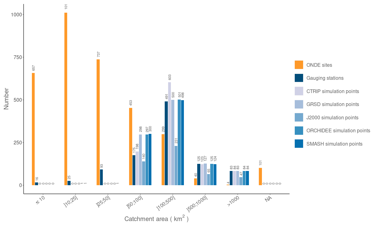
Figure G1 Frequency distribution of the number of ONDE sites, the 1008 gauging stations selected from the HydroPortail database, and the 1008 simulation points from Explore2 as a function of catchment area. NA: missing values.

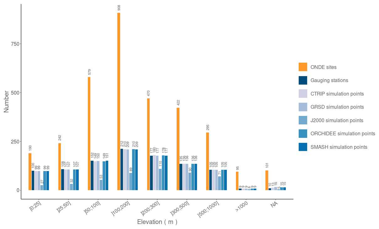
Figure G2 Frequency distribution of the number of ONDE sites, the 1008 gauging stations selected from the HydroPortail database, and the 1008 simulation points from Explore2 as a function of elevation NA: missing value.

Figure G3 Strahler index of ONDE sites. NA: missing value.

Appendix H: Model performance using observed discharge data from gauging stations as predictors

Over the observation period (2012–2022), logistic regression models estimate the PFI values at HER2 scale (Fig. 4). The median observed PFI across all HER2s and all campaigns is 14.3 % (Q1–Q3: 8.4–20.3), while the logistic regression models yield a median value of 14.4 % (Q1–Q3: 8.5–20.4). With results of the leave-one-year-out cross-validation, the models explain 73 % of the PFI variability according to the NSE (Q1–Q3: 64 %–84 %) (Table 1; Fig. H2), the KGE exceeds 80 % in 50 out of 75 HER2s (Fig. H2), and the bias is very low.

The models are also able to describe the inter-annual variability with the alternation of dry and wet years (Fig. H1). The median KGE and NSE scores remain above 0.71 during k-fold validations considering dry, intermediate, and wet years for calibration. RMSE and MAE values do not increase much when the calibration dataset is stratified based on climate conditions, which indicates that the proposed model is quite robust against climate variations under current conditions.

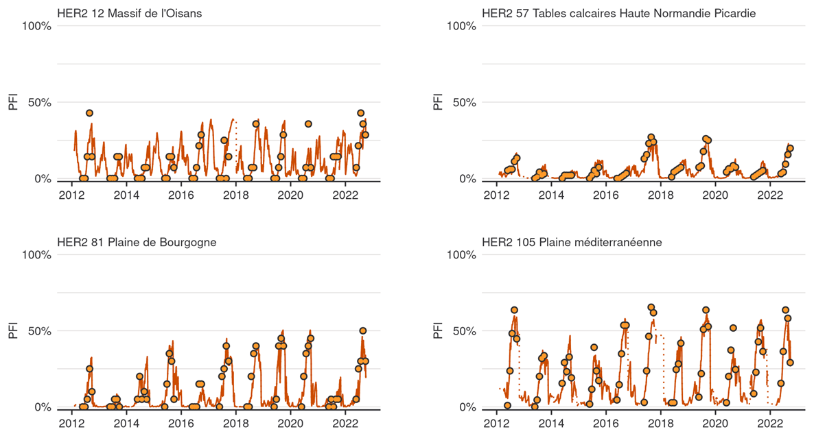
Figure H1 Time series of PFI in HER2-13, HER2-57, HER2-81, and HER2-105. Points and lines respectively represent the PFI derived from the ONDE network and the PFI estimated by the logistic regression models using discharge data from gauging stations during the calibration period (2012–2022).

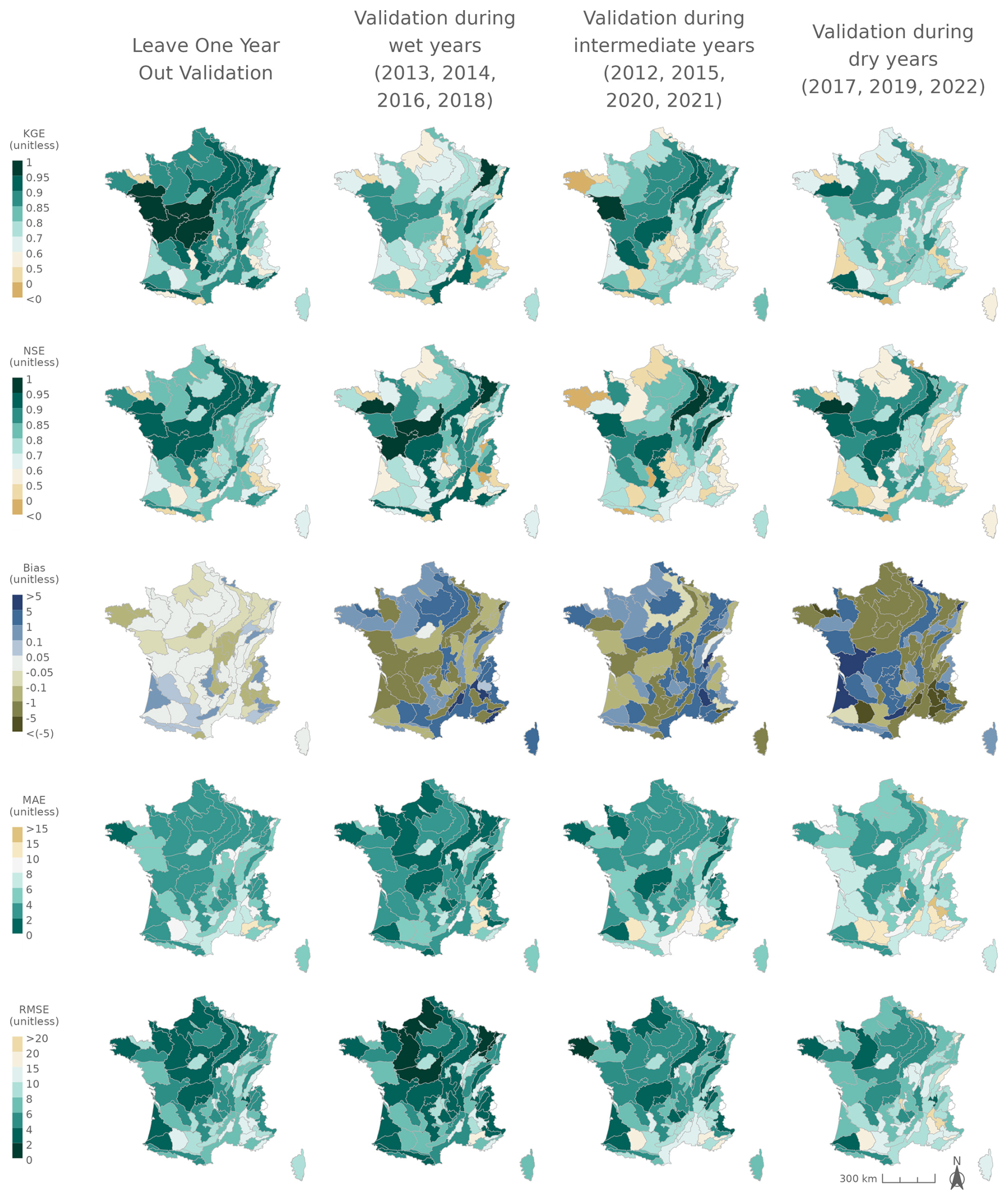
Figure H2 Kling–Gupta efficiency (KGE, line 1), Nash–Sutcliffe model efficiency coefficient (NSE, line 2), bias (line 3), mean absolute error (MAE, line 4), and root-mean-square error (RMSE, line 5) over the calibration period (2012–2022).

Table H1 Validation results of drying probability predictions at the HER2 scale using observed flows from the 1008 gauging stations from the HYDRO database. The results correspond to the inter-HER medians, quartiles, and minimum and maximum values. The leave-one-year-out analysis results are obtained by averaging the validation metrics computed for each year.

Drying probability: percentage of ONDE sites in a dry state computed for each HER2, averaged by month; Q1–Q3: first and third quartiles; Min: minimum; Max: maximum.

Appendix I: Model performance using discharge data simulated with SAFRAN

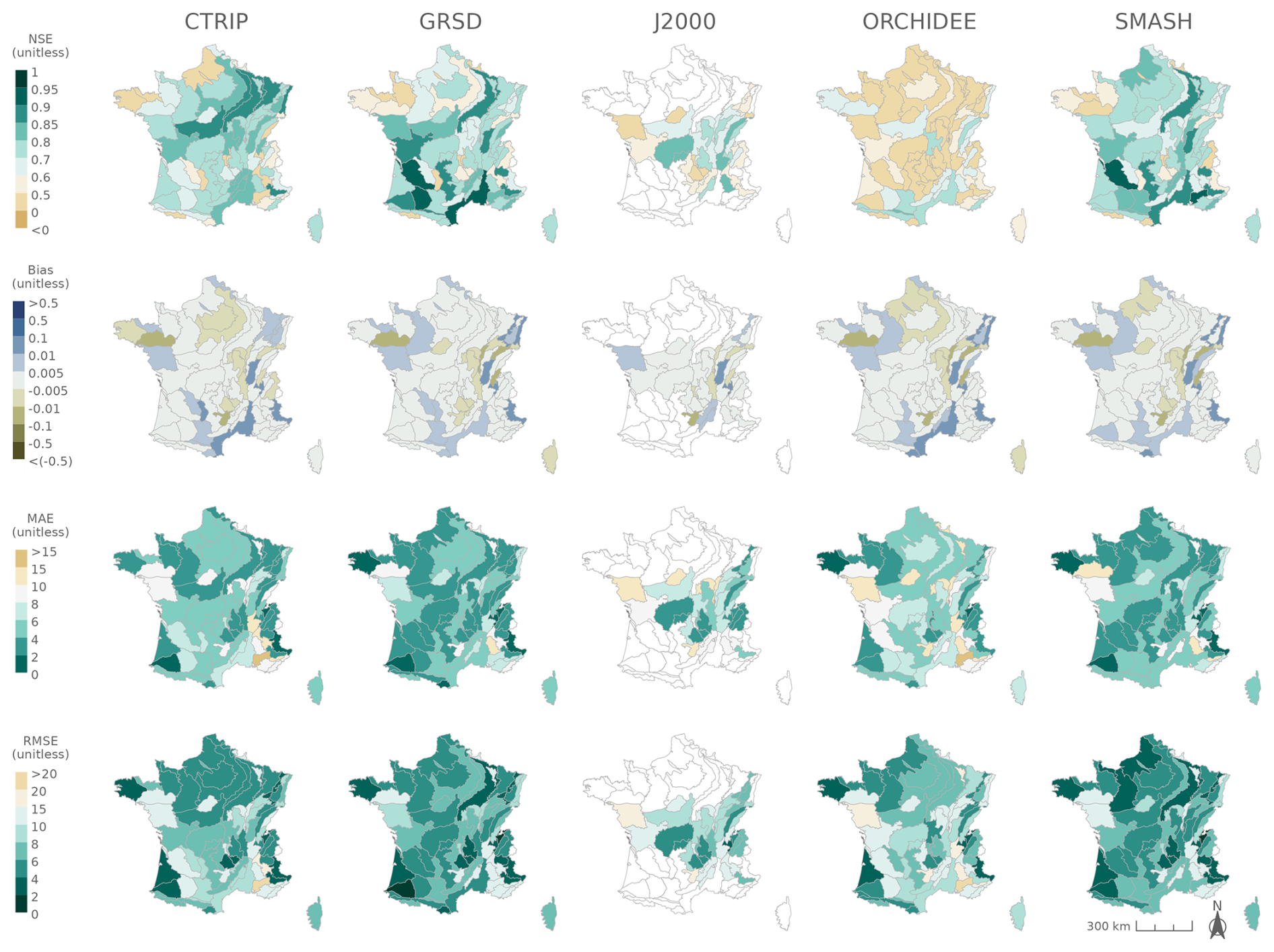
Figure I1 Nash–Sutcliffe model efficiency (NSE) coefficient (line 1), bias (line 2), mean absolute error (MAE, line 3), and root-mean-square error (RMSE, line 4) assessing the calibration of logistic regression using discharge data simulated with SAFRAN data available during the calibration period (2012–2022).

Appendix J: Application to 21st century PFI modelling

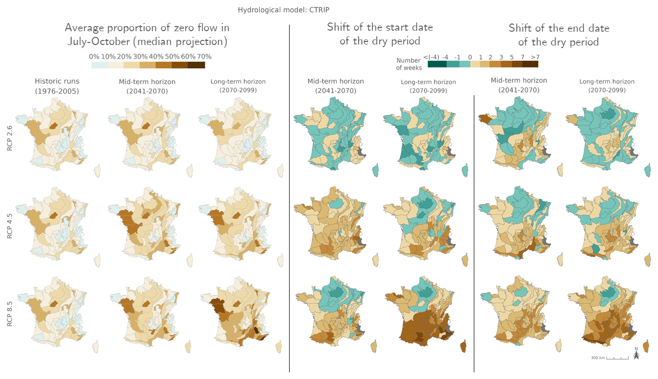
Figure J1 Ensemble median mPFI_7–10 (columns 1 to 3) and ensemble median shift of the start date Tf (columns 4 and 5) and the end date Tl (columns 6 and 7) of the dry period over the two periods 2041–2070 and 2070–2099 under the three RCPs for the CTRIP hydrological model, relative to the baseline period 1976–2005. The shift, expressed in weeks, takes a positive value when the duration of the dry period increases. Grey HER2s had no period with a PFI >20 % during the reference period.

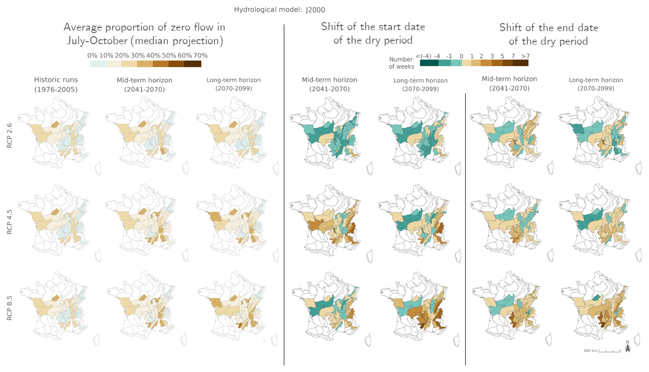
Figure J2 Ensemble median mPFI_7–10 (columns 1 to 3) and ensemble median shift of the start date Tf (columns 4 and 5) and the end date Tl (columns 6 and 7) of the dry period over the two periods 2041–2070 and 2070–2099 under the three RCPs for the J2000 hydrological model, relative to the baseline period 1976–2005. The shift, expressed in weeks, takes a positive value when the duration of the dry period increases. Grey HER2s had no period with a PFI >20 % during the reference period.

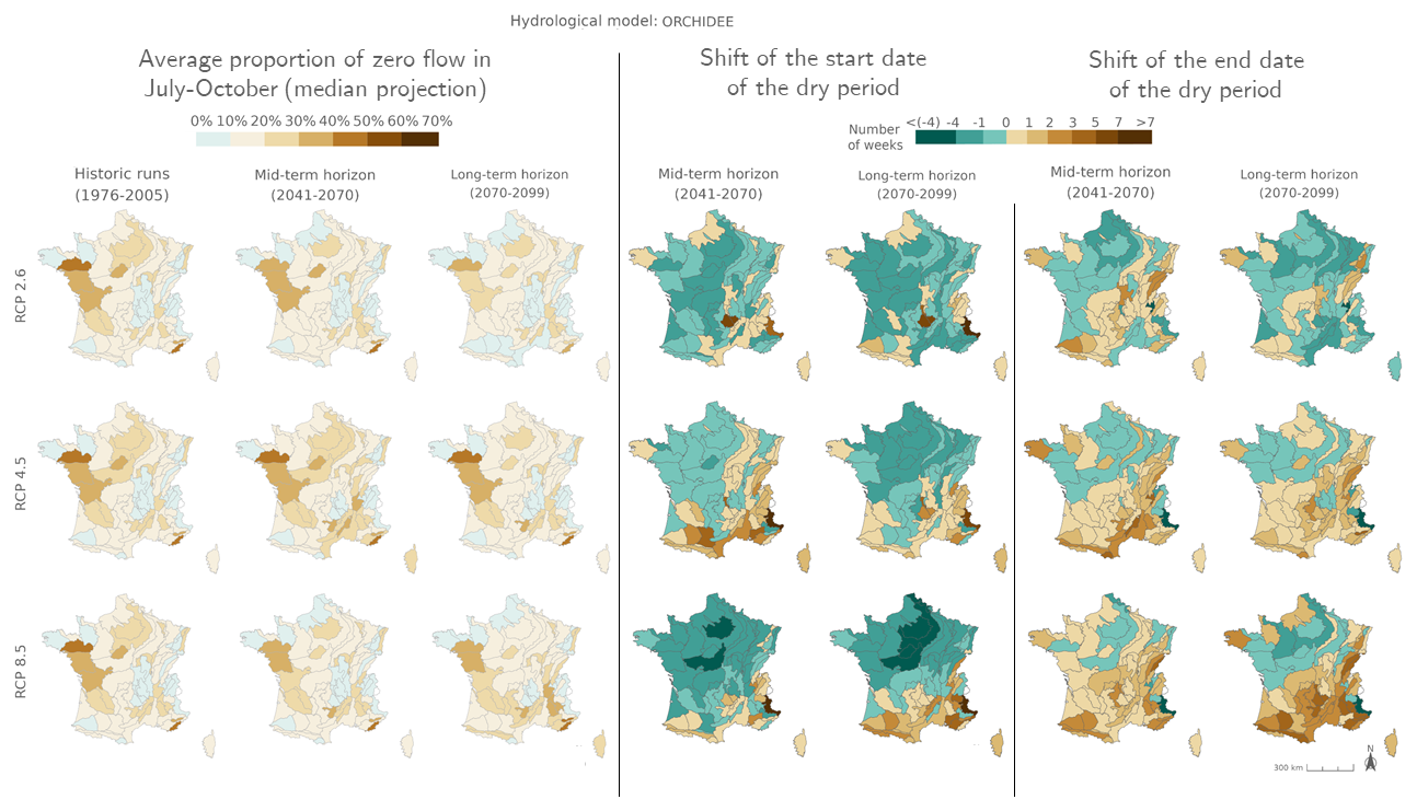
Figure J3 Ensemble median mPFI_7–10 (columns 1 to 3) and ensemble median shift of the start date Tf (columns 4 and 5) and the end date Tl (columns 6 and 7) of the dry period over the two periods 2041–2070 and 2070–2099 under the three RCPs for the ORCHIDEE hydrological model, relative to the baseline period 1976–2005. The shift, expressed in weeks, takes a positive value when the duration of the dry period increases. Grey HER2s had no period with a PFI >20 % during the reference period.

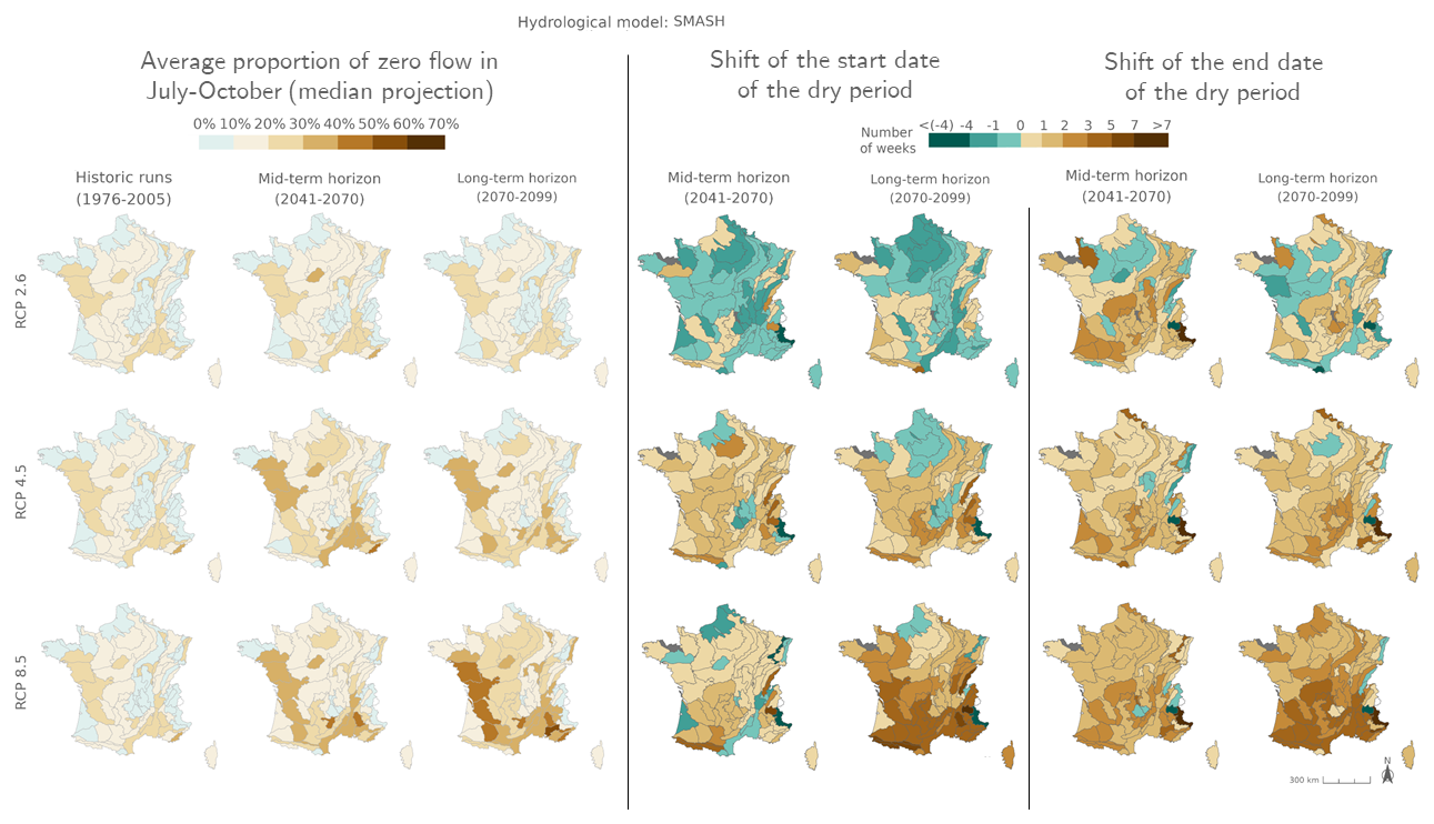
Figure J4 Ensemble median mPFI_7–10 (columns 1 to 3) and ensemble median shift of the start date Tf (columns 4 and 5) and the end date Tl (columns 6 and 7) of the dry period over the two periods 2041–2070 and 2070–2099 under the three RCPs for the SMASH hydrological model, relative to the baseline period 1976–2005. The shift, expressed in weeks, takes a positive value when the duration of the dry period increases. Grey HER2s had no period with a PFI >20 % during the reference period.

J1 Narratives

The following figures present time series of the evolution of PFI dynamics at different horizons and under different RCP scenarios for each hydrological model in HER2-12, HER2-57, HER2-81, and HER2-105. Four contrasting scenarios were highlighted among the Explore2 climate projections to illustrate a diversity of potential changes under RCP8.5. These story lines range from “Strong warming and strong summer (and annual) drying”, selected as one of the most extreme climate projections, to “Moderate warming and precipitation change” with less pronounced alterations, with two alternative projections named “Dry all year, reduced winter recharge” and “Hot and humid all seasons”. They are also illustrated here to present distinct hydrological nuances.

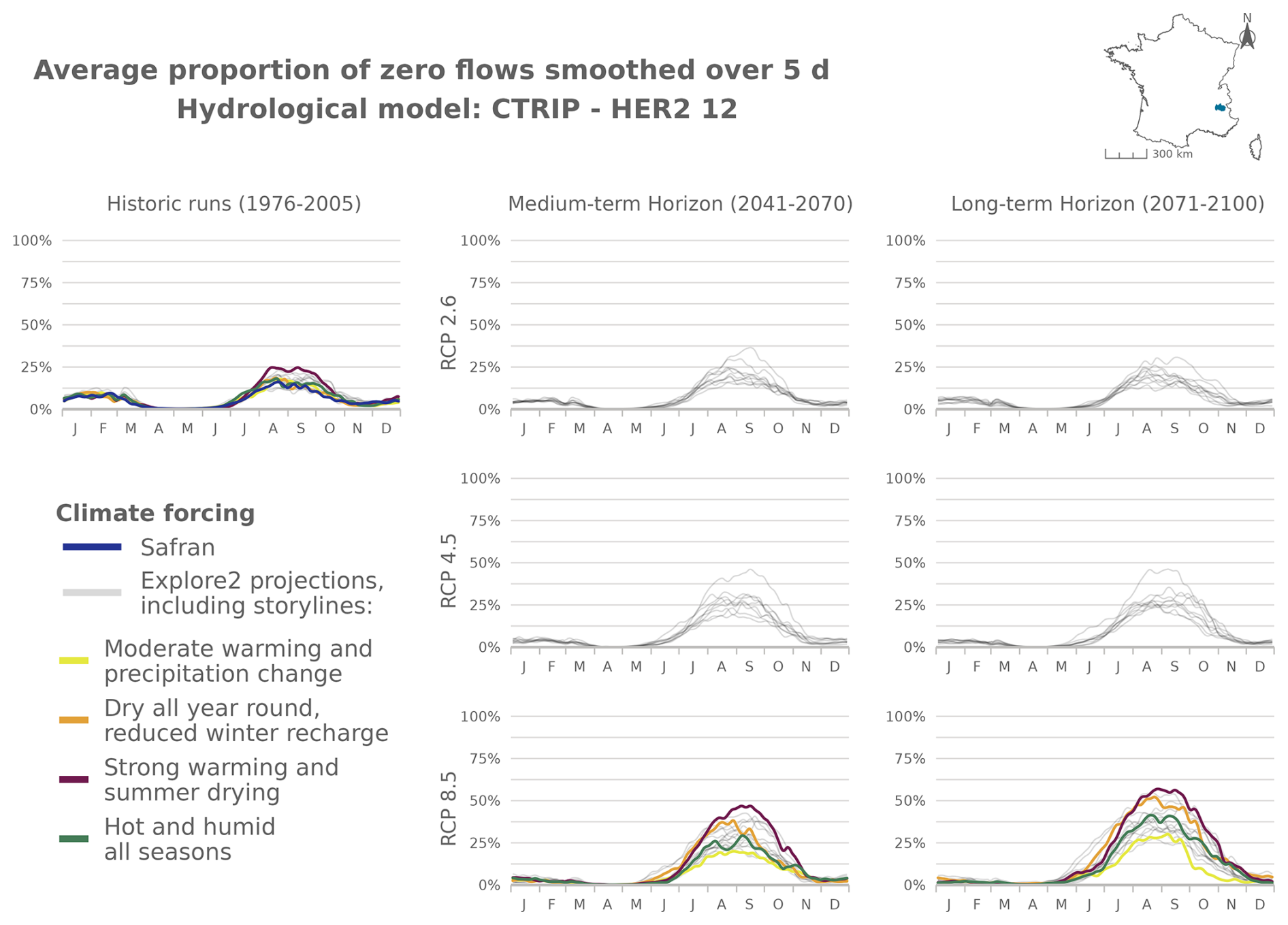
Figure J5 Time series of the evolution of PFI dynamics at different horizons under different RCP scenarios for the CTRIP hydrological model in HER2-12 (d = day).

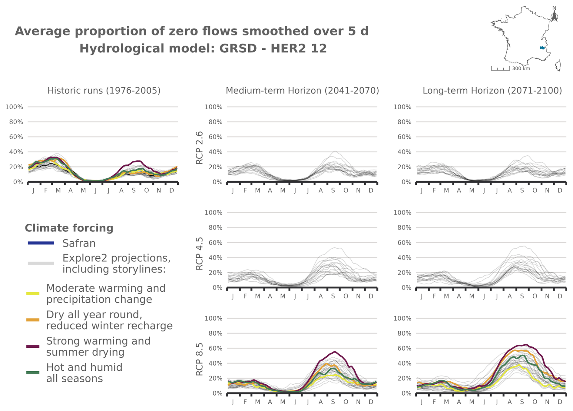
Figure J6 Time series of the evolution of PFI dynamics at different horizons under different RCP scenarios for the GRSD hydrological model in HER2-12.

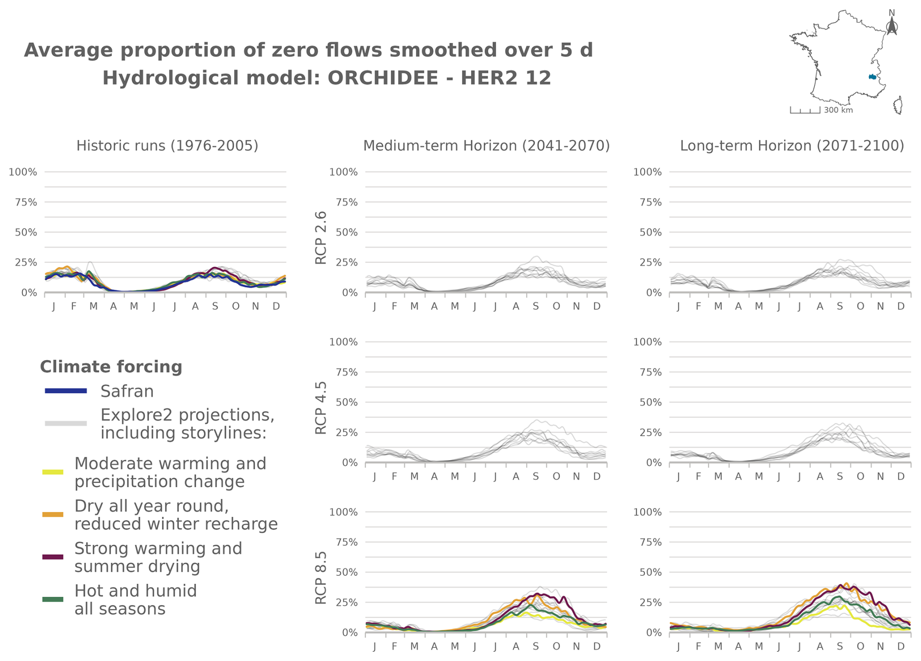
Figure J7 Time series of the evolution of PFI dynamics at different horizons under different RCP scenarios for the ORCHIDEE hydrological model in HER2-12.

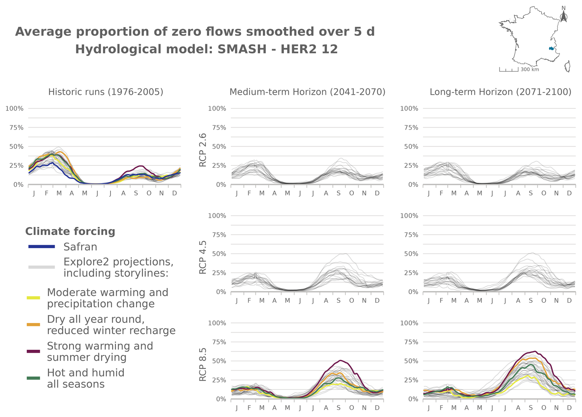
Figure J8 Time series of the evolution of PFI dynamics at different horizons under different RCP scenarios for the SMASH hydrological model in HER2-12.

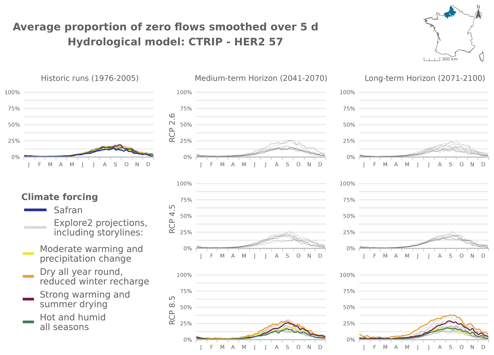
Figure J9 Time series of the evolution of PFI dynamics at different horizons under different RCP scenarios for the CTRIP hydrological model in HER2-57.

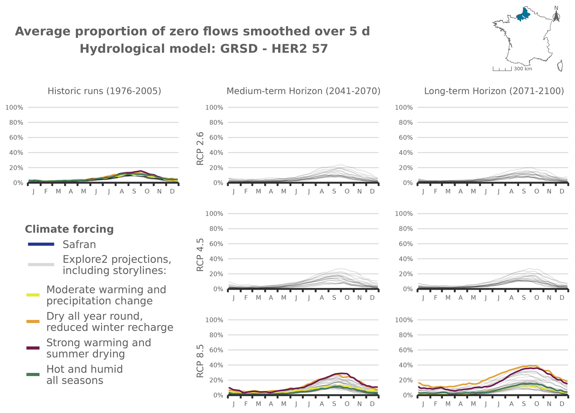
Figure J10 Time series of the evolution of PFI dynamics at different horizons under different RCP scenarios for the GRSD hydrological model in HER2-57.

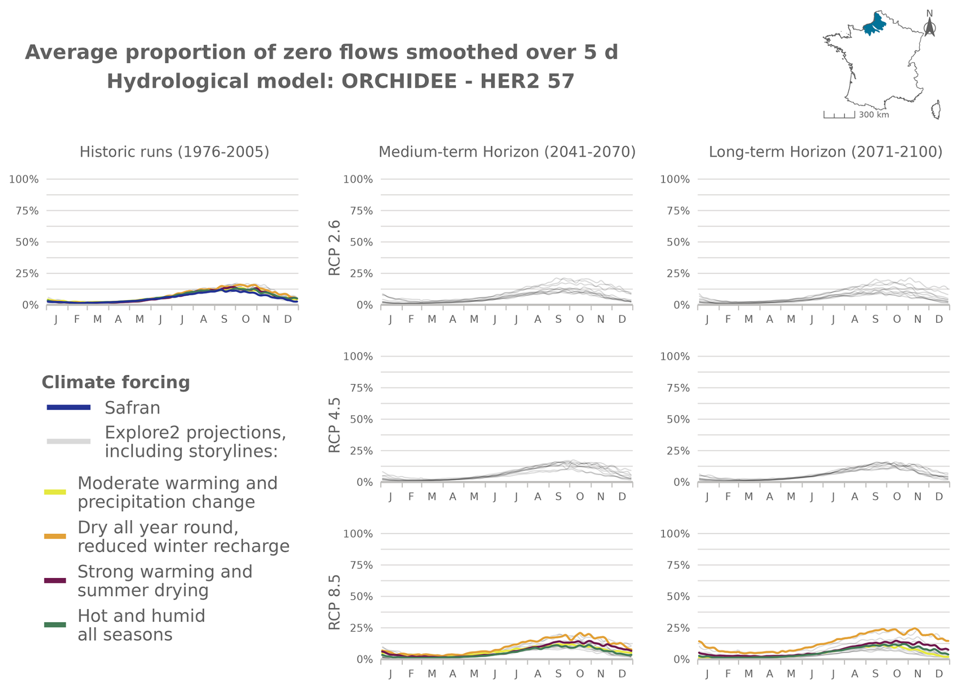
Figure J11 Time series of the evolution of PFI dynamics at different horizons under different RCP scenarios for the ORCHIDEE hydrological model in HER2-57.

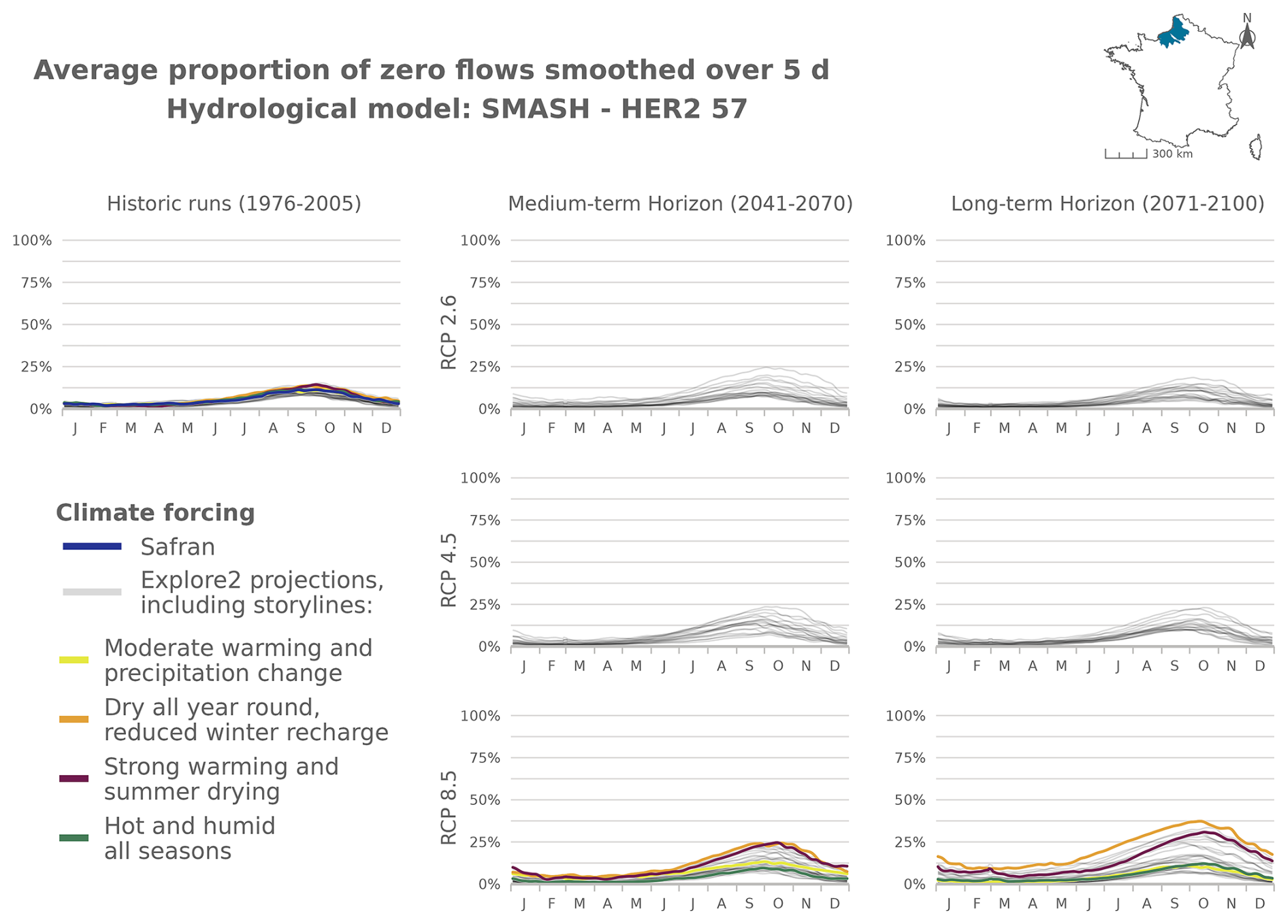
Figure J12 Time series of the evolution of PFI dynamics at different horizons under different RCP scenarios for the SMASH hydrological model in HER2-57.

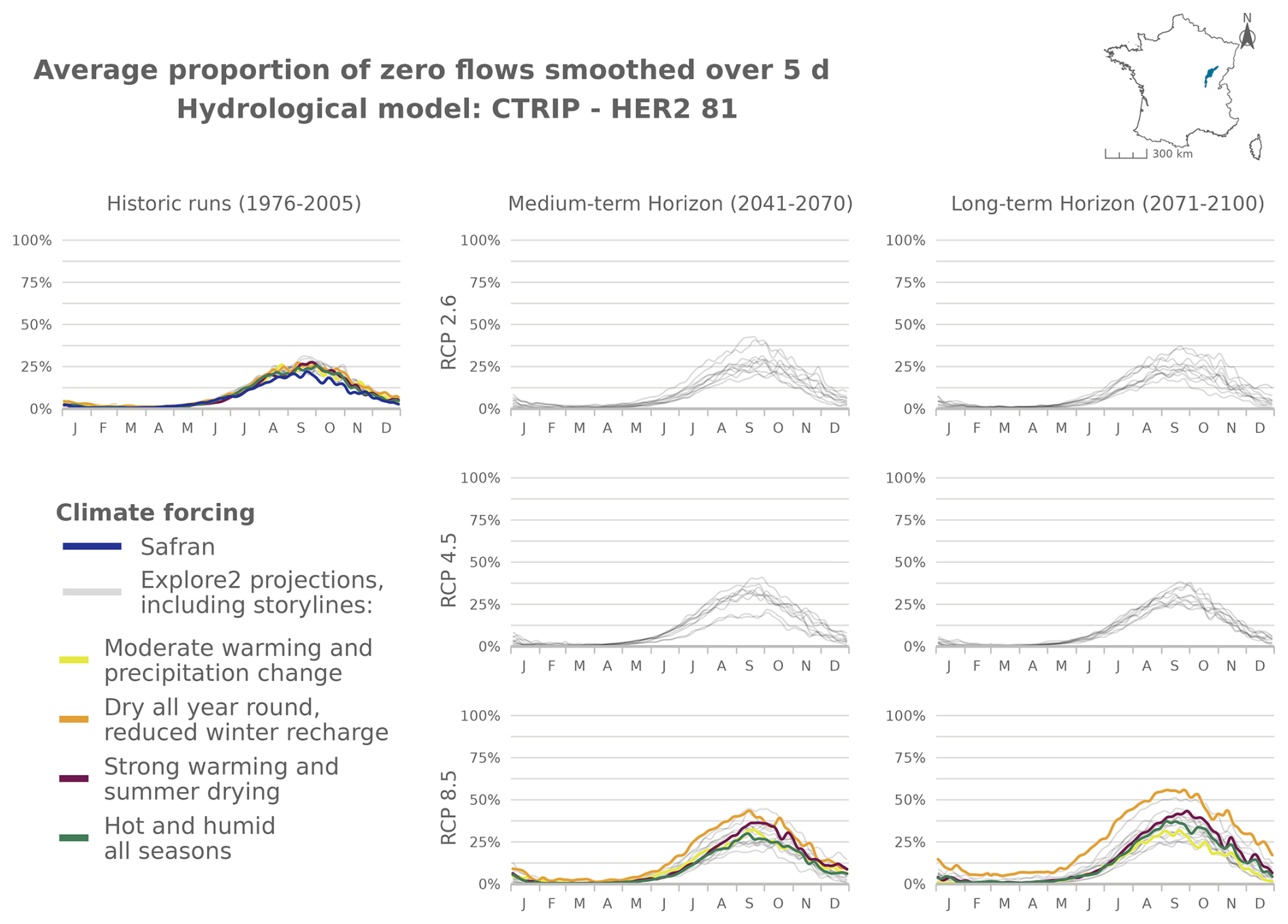
Figure J13 Time series of the evolution of PFI dynamics at different horizons under different RCP scenarios for the CTRIP hydrological model in HER2-81.

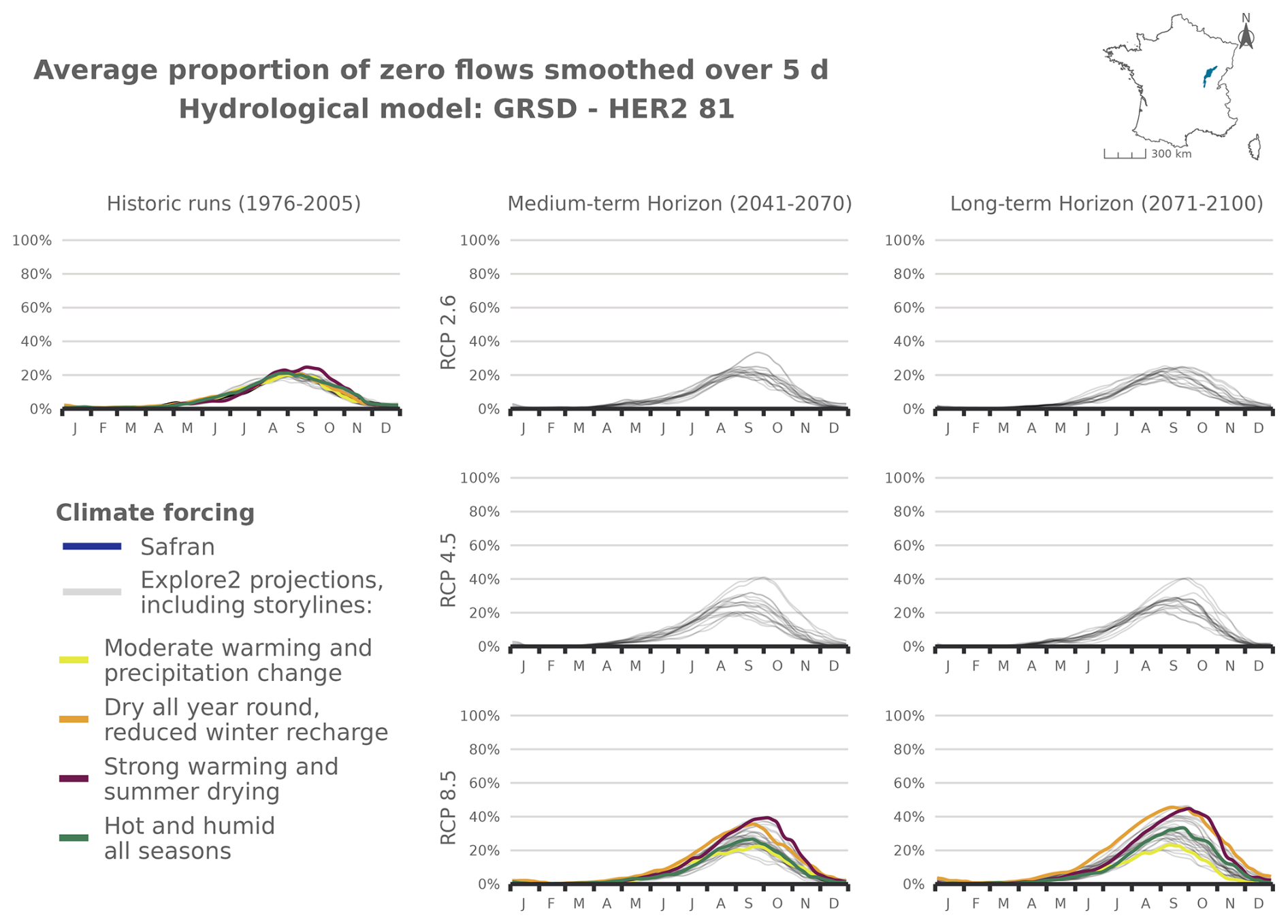
Figure J14 Time series of the evolution of PFI dynamics at different horizons under different RCP scenarios for the GRSD hydrological model in HER2-81.

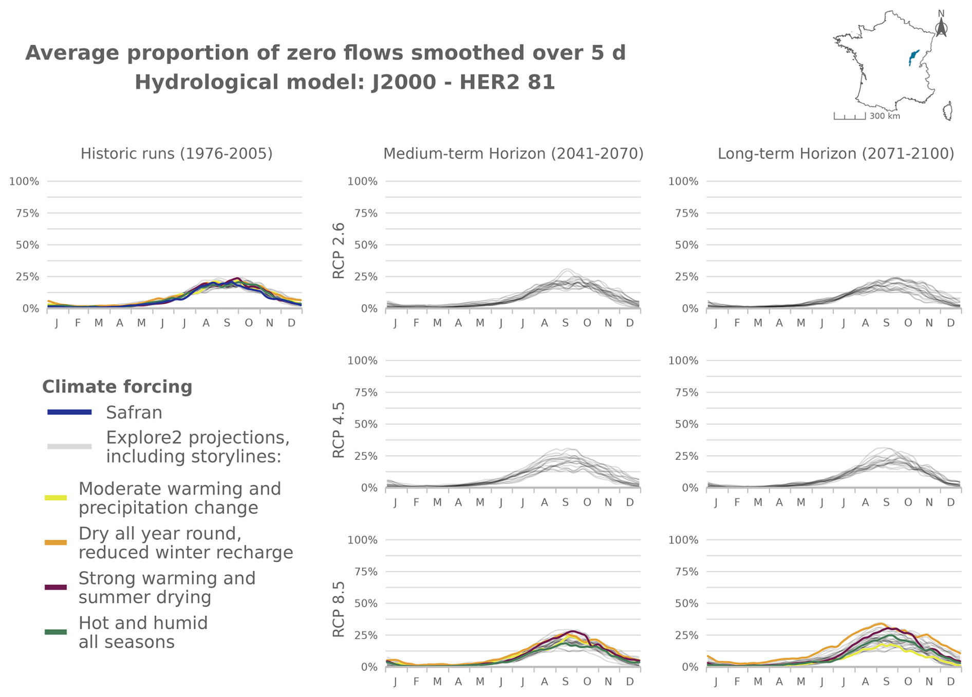
Figure J15 Time series of the evolution of PFI dynamics at different horizons under different RCP scenarios for the J2000 hydrological model in HER2-81.

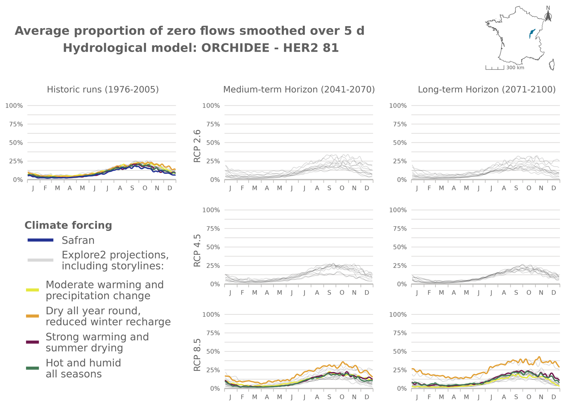
Figure J16 Time series of the evolution of PFI dynamics at different horizons under different RCP scenarios for the ORCHIDEE hydrological model in HER2-81.

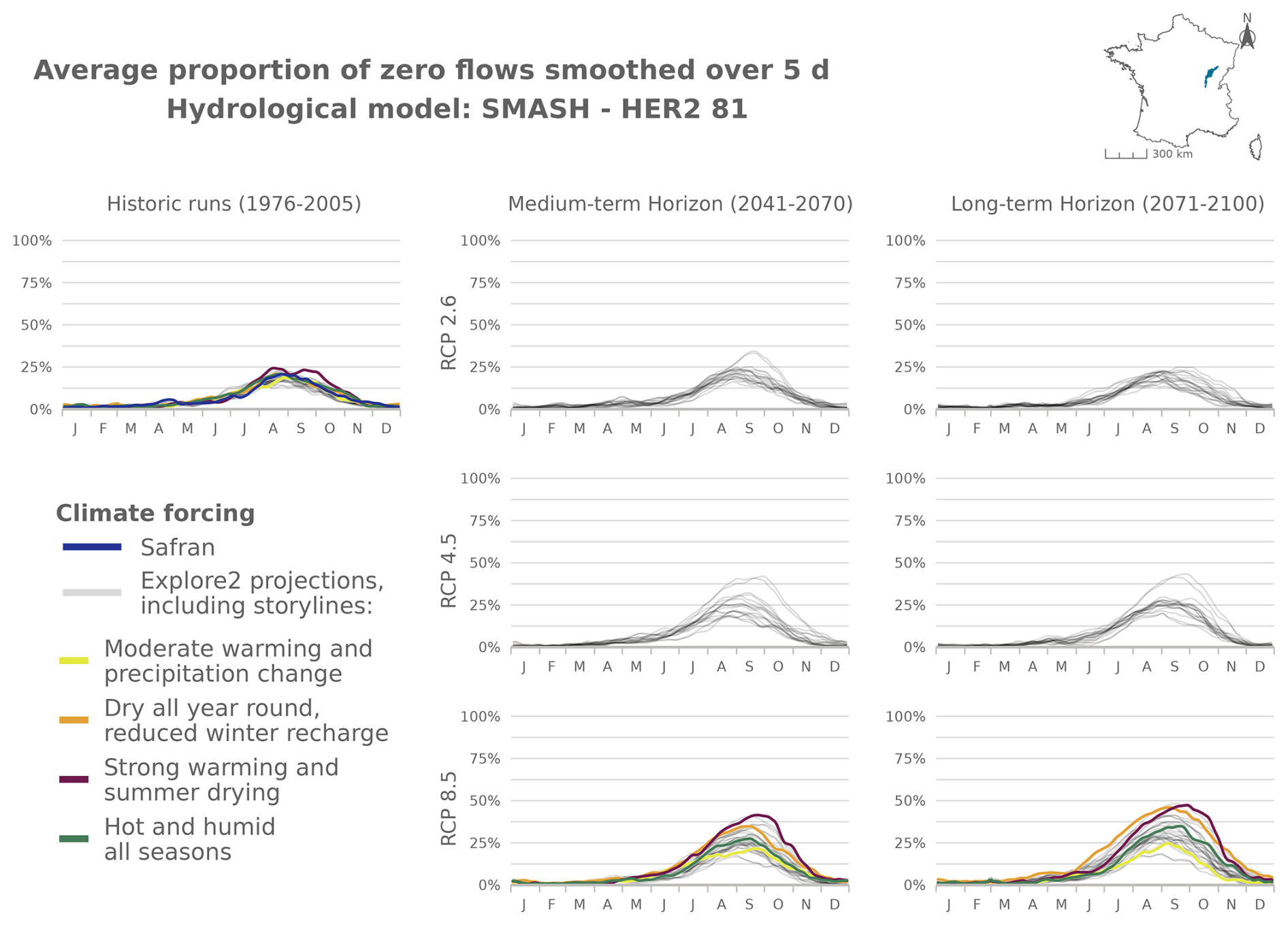
Figure J17 Time series of the evolution of PFI dynamics at different horizons under different RCP scenarios for the SMASH hydrological model in HER2-81.

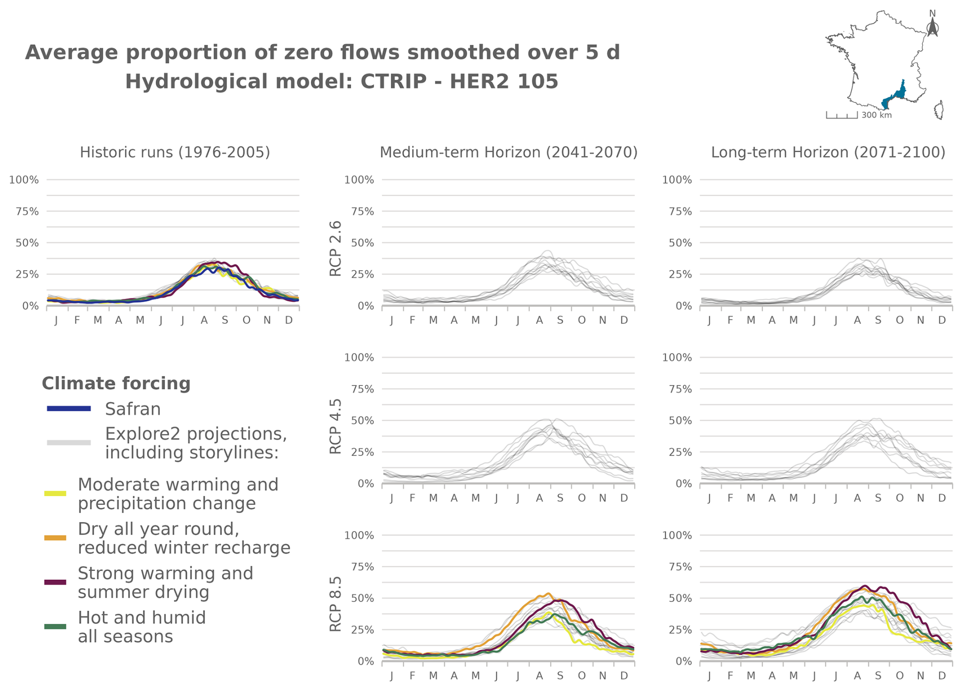
Figure J18 Time series of the evolution of PFI dynamics at different horizons under different RCP scenarios for the CTRIP hydrological model in HER2-105.

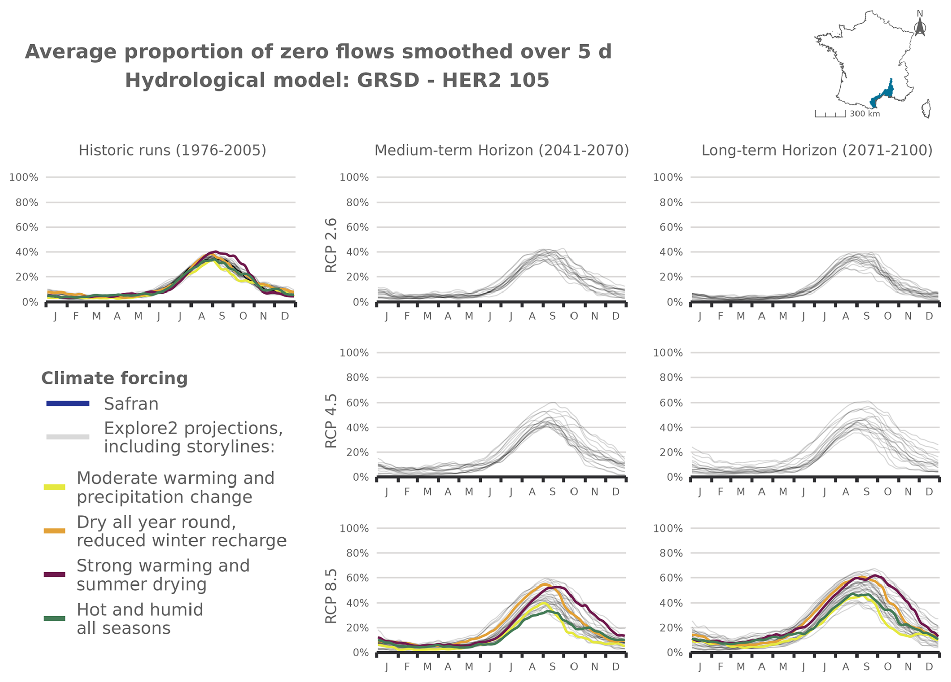
Figure J19 Time series of the evolution of PFI dynamics at different horizons under different RCP scenarios for the GRSD hydrological model in HER2-105.

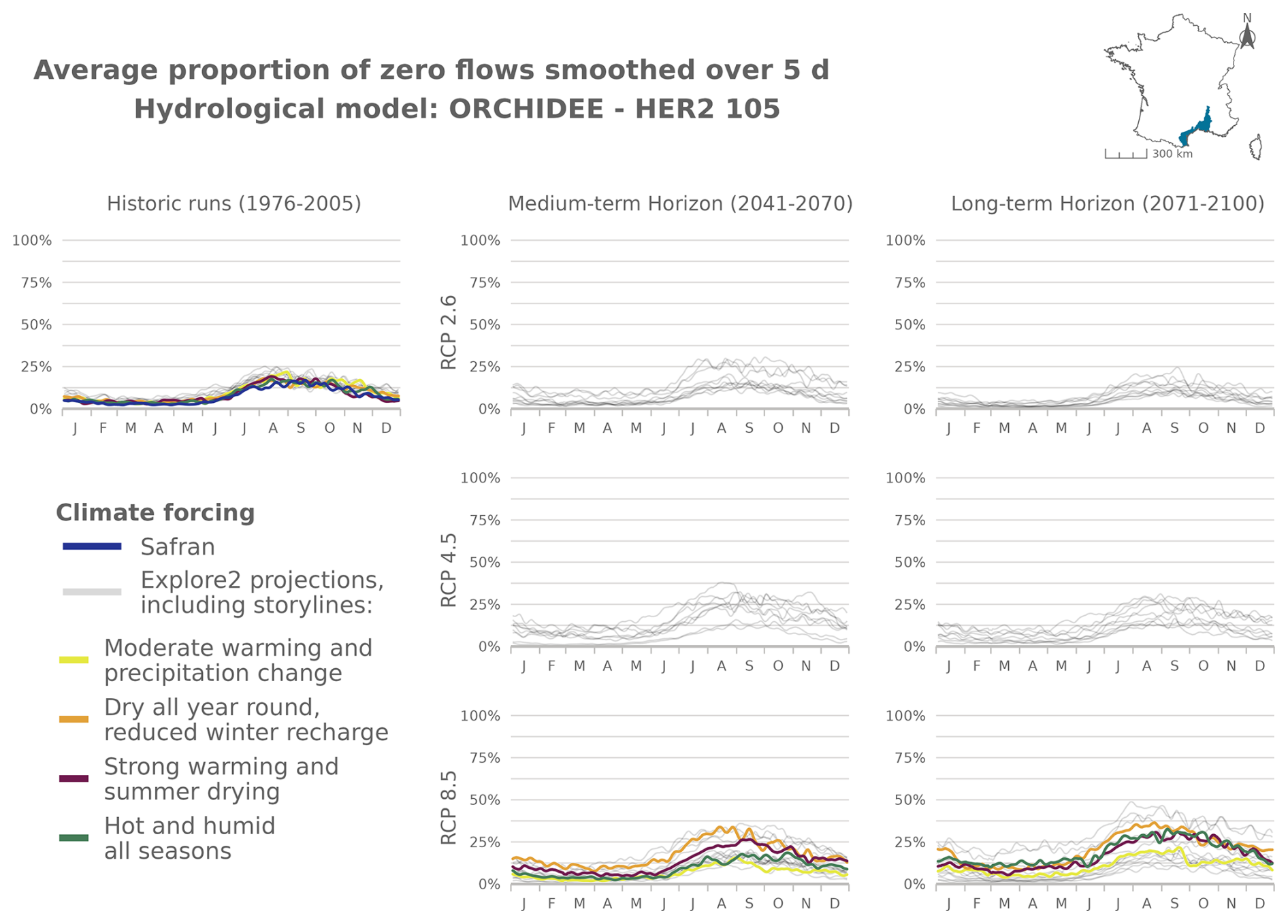
Figure J20 Time series of the evolution of PFI dynamics at different horizons under different RCP scenarios for the ORCHIDEE hydrological model in HER2-105.

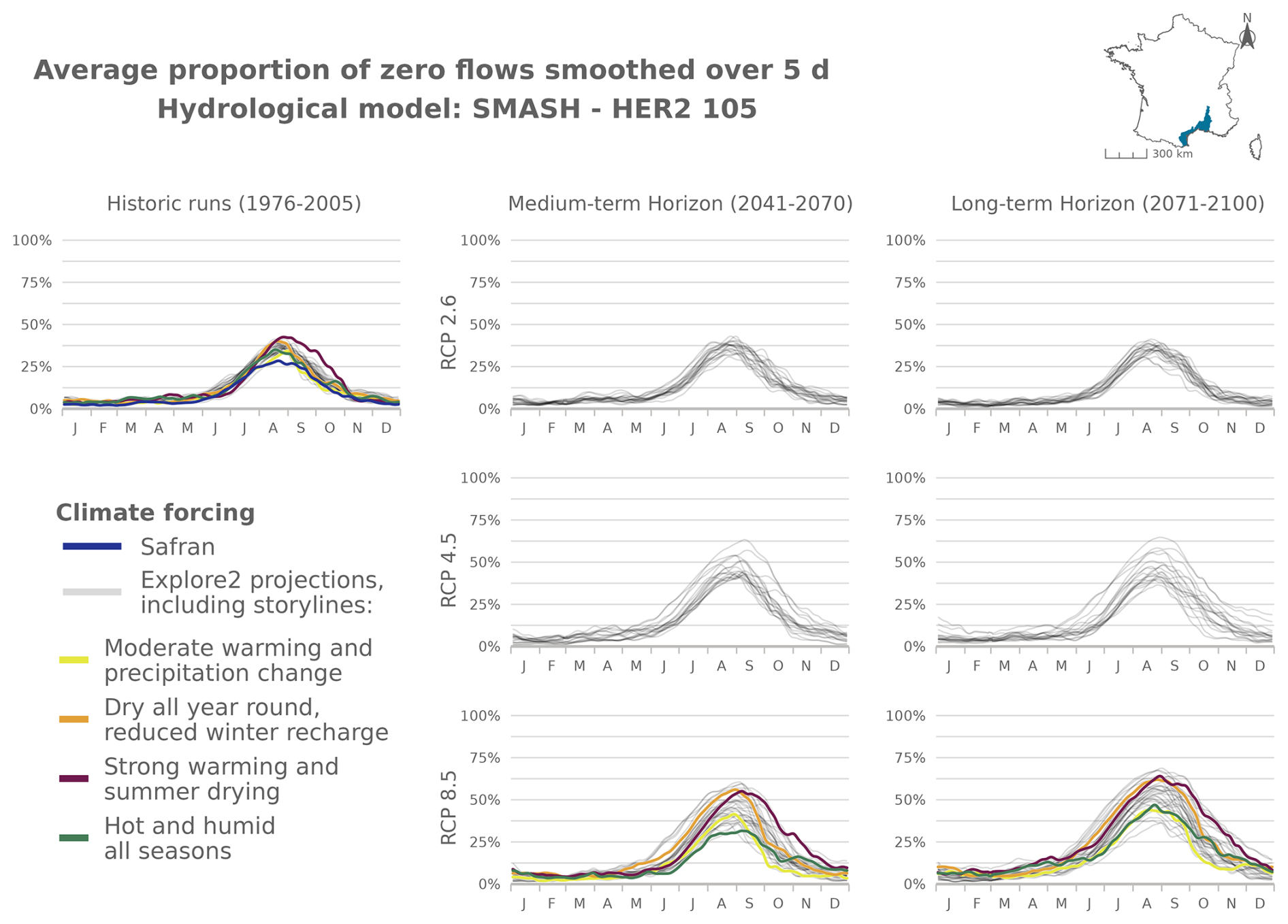
Figure J21 Time series of the evolution of PFI dynamics at different horizons under different RCP scenarios for the SMASH hydrological model in HER2-105.

Appendix K: Agreement between changes under RCP4.5

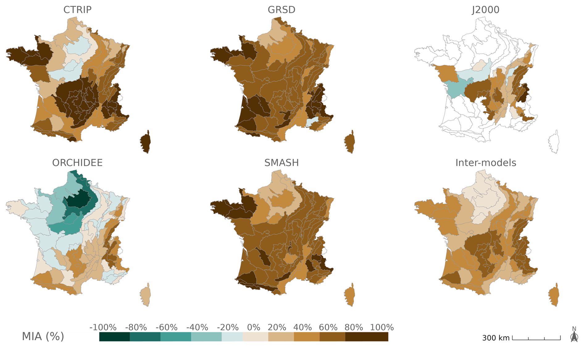
Figure K1 Agreement between projections of mPFI_7–10 for each hydrological model and inter-model agreement on the change signal of mPFI_7–10 under the RCP4.5 scenario.